Investigation of the North Atlantic Oscillation and Indian Ocean Dipole Influence on Precipitation in Turkey with Cross-Spectral Analysis


Abstract
:1. Introduction
2. Material and Method
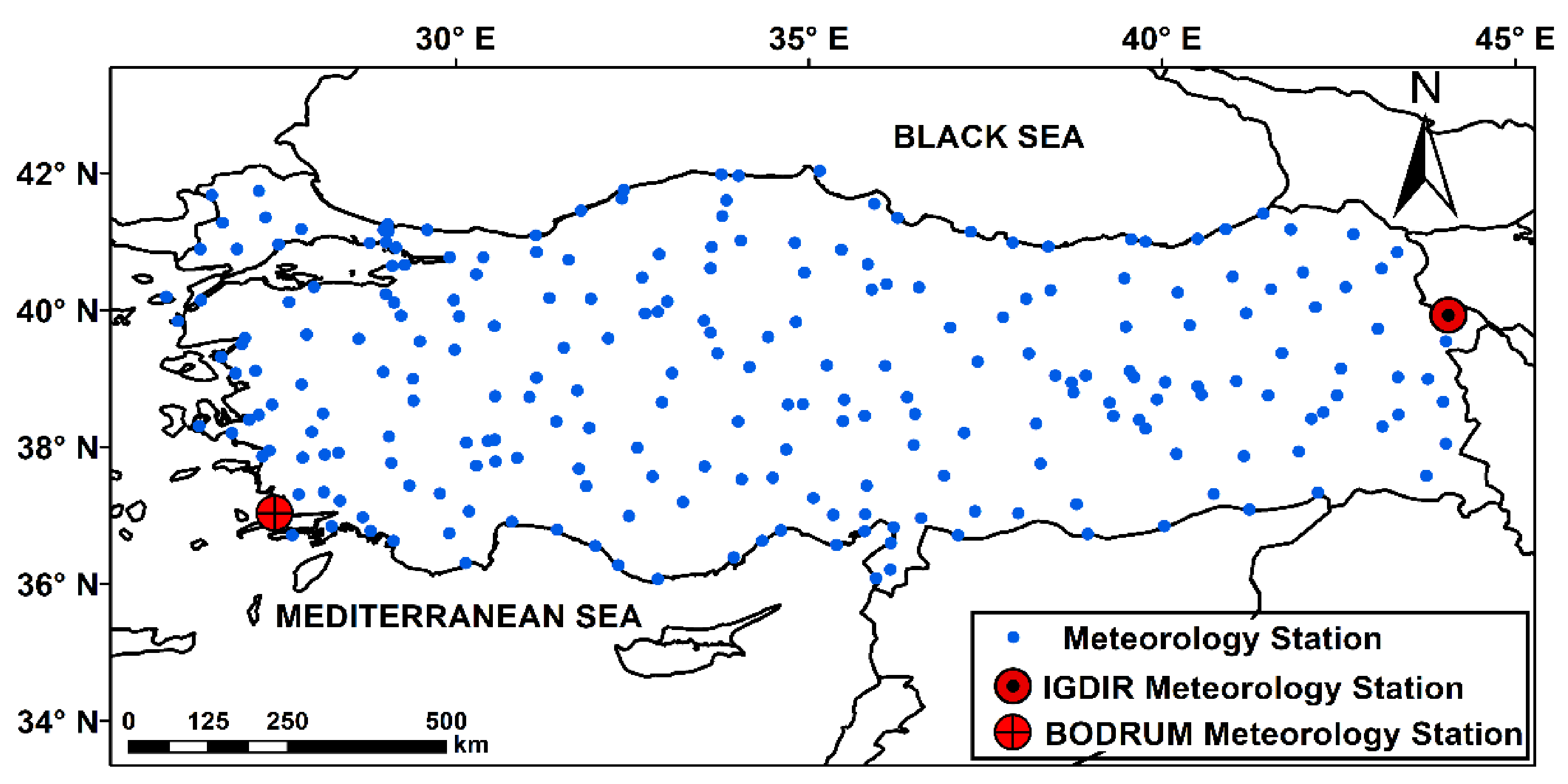
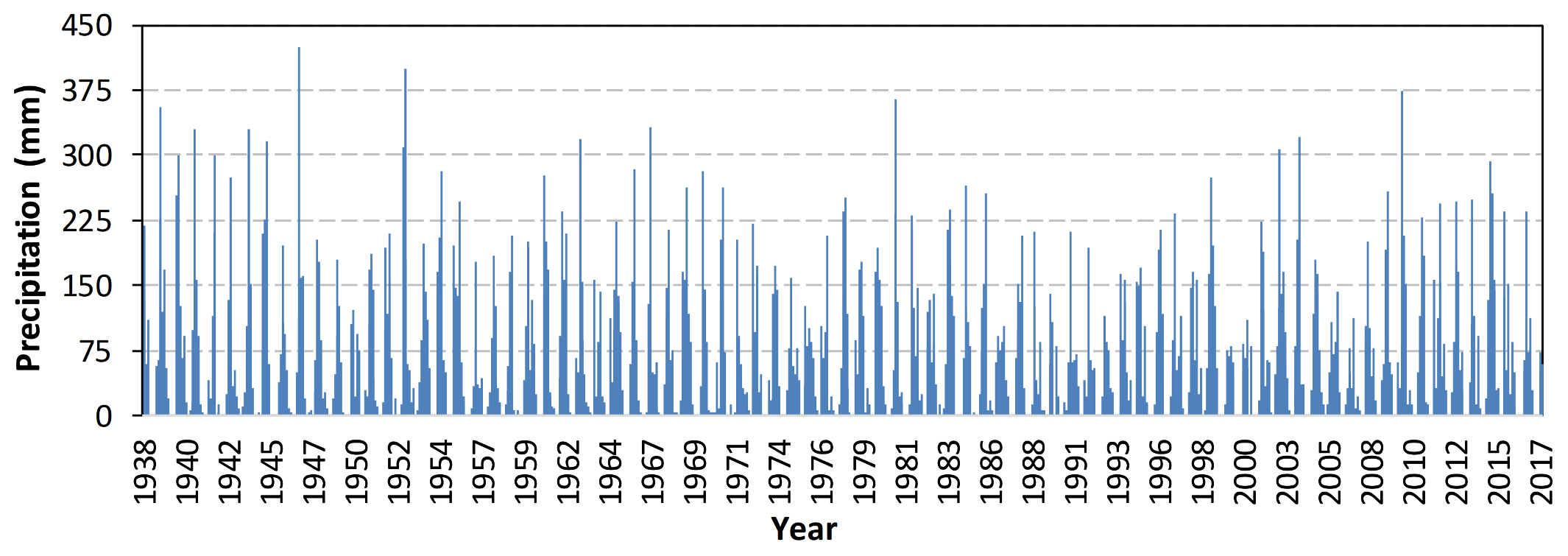
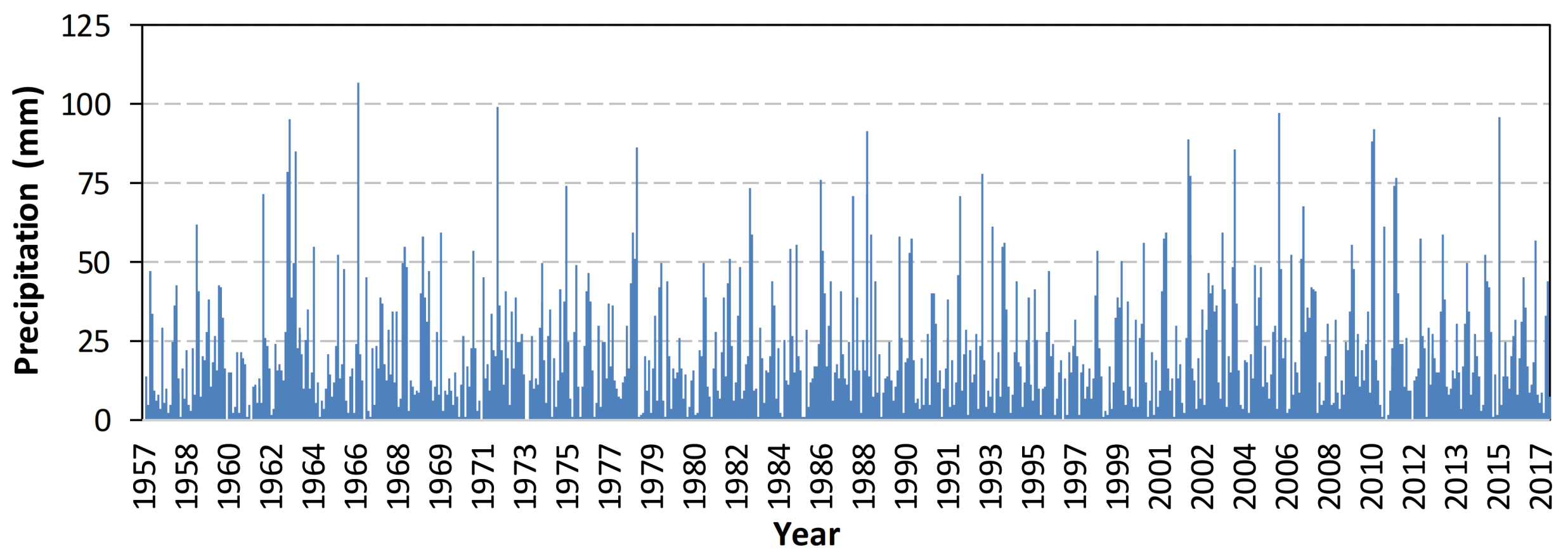
2.1. Meteorology Stations and Precipitation Data
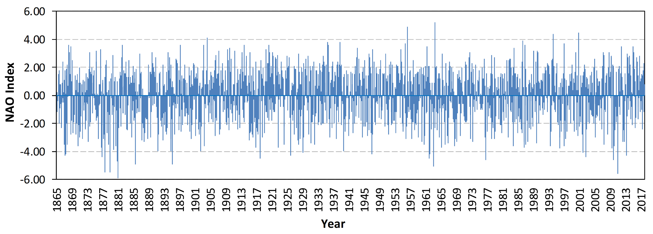
2.2. NAO Data
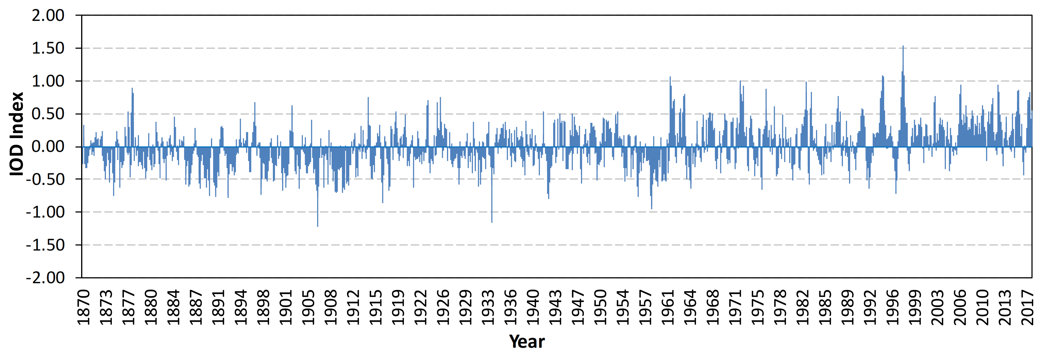
2.3. IOD Data
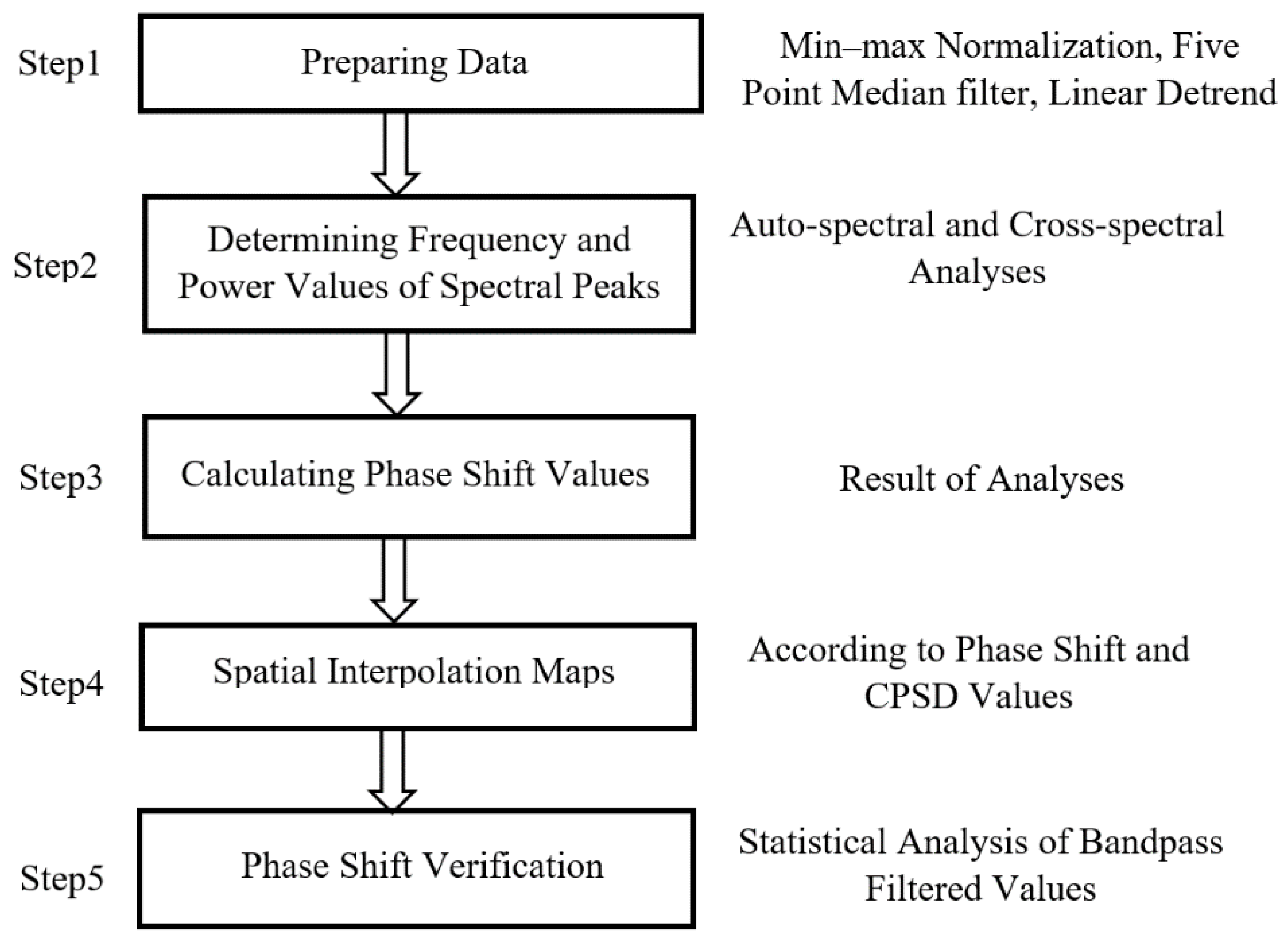
2.4. Auto-Spectral and Cross-Spectral Analysis
3. Results and Discussion
4. Conclusions
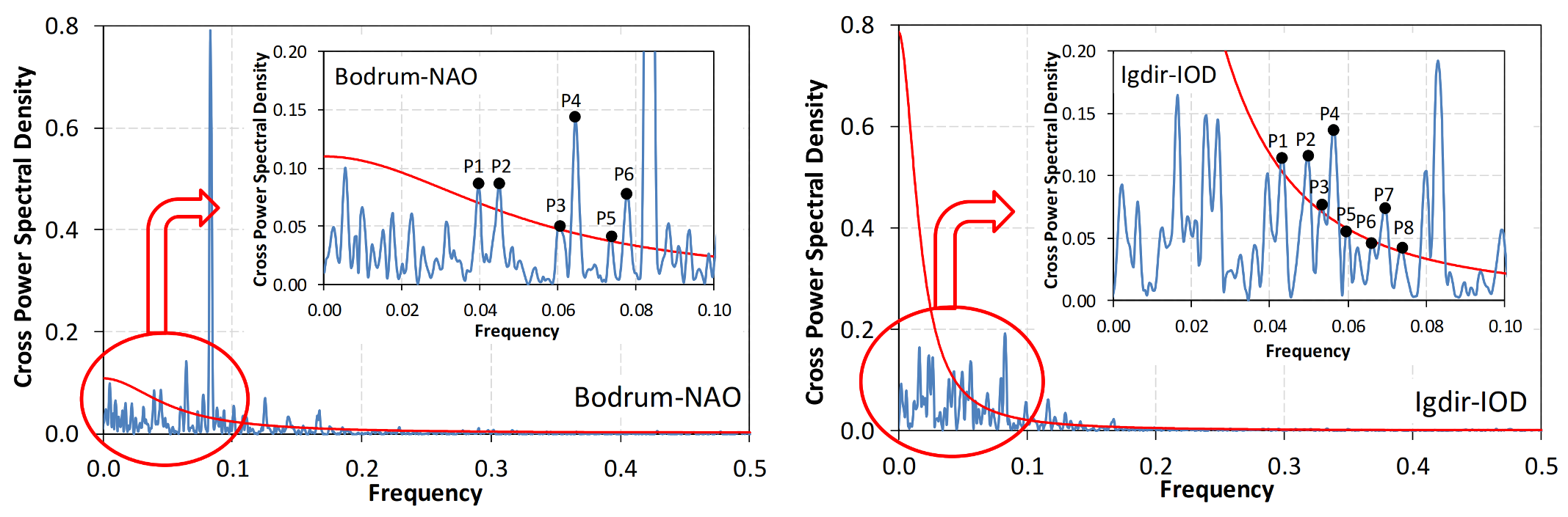
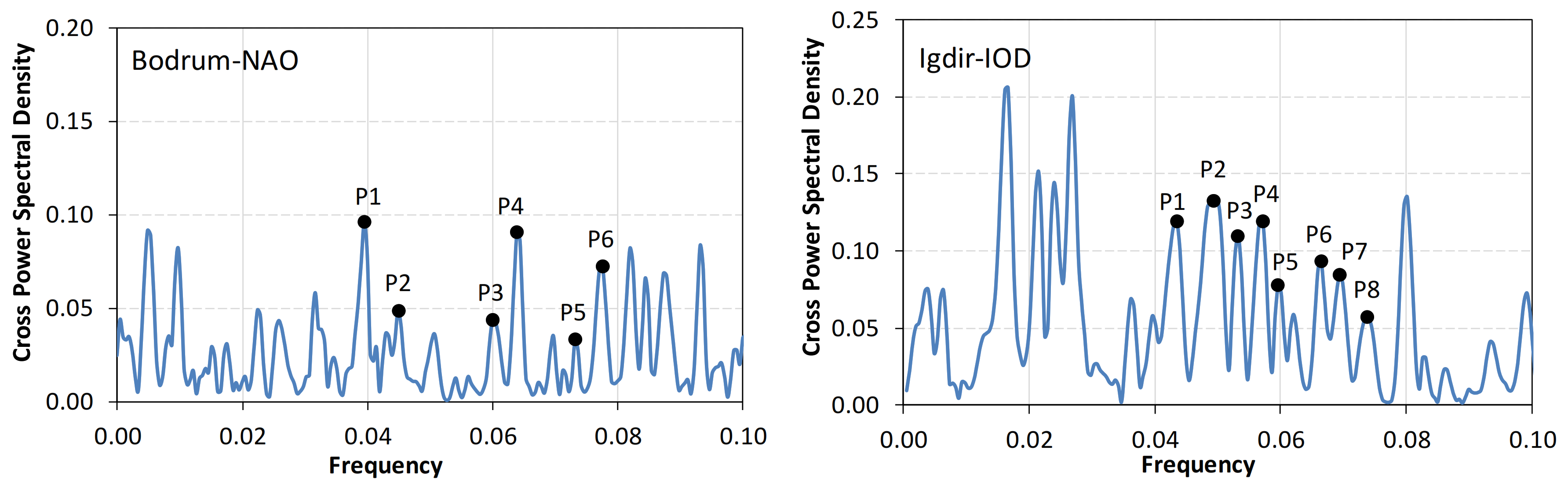
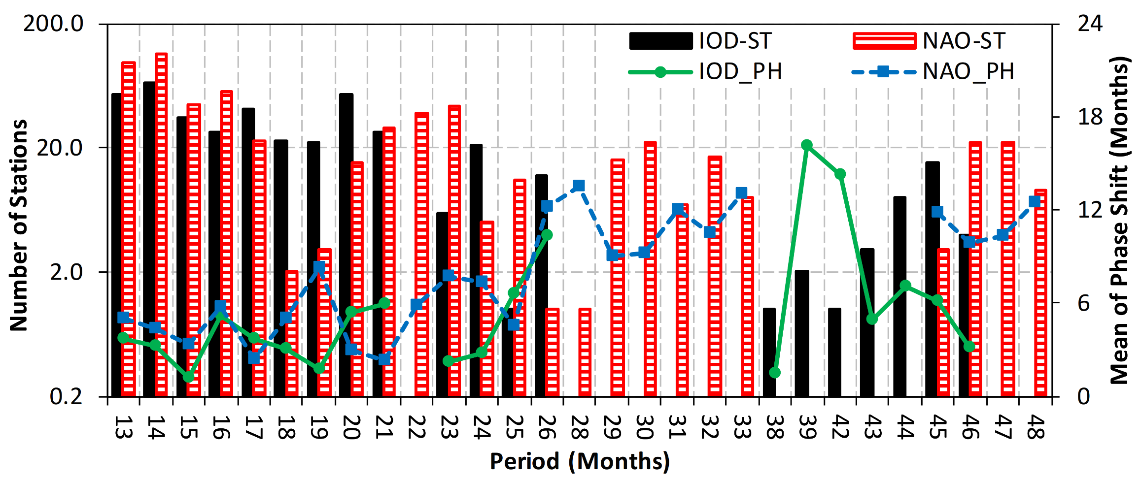
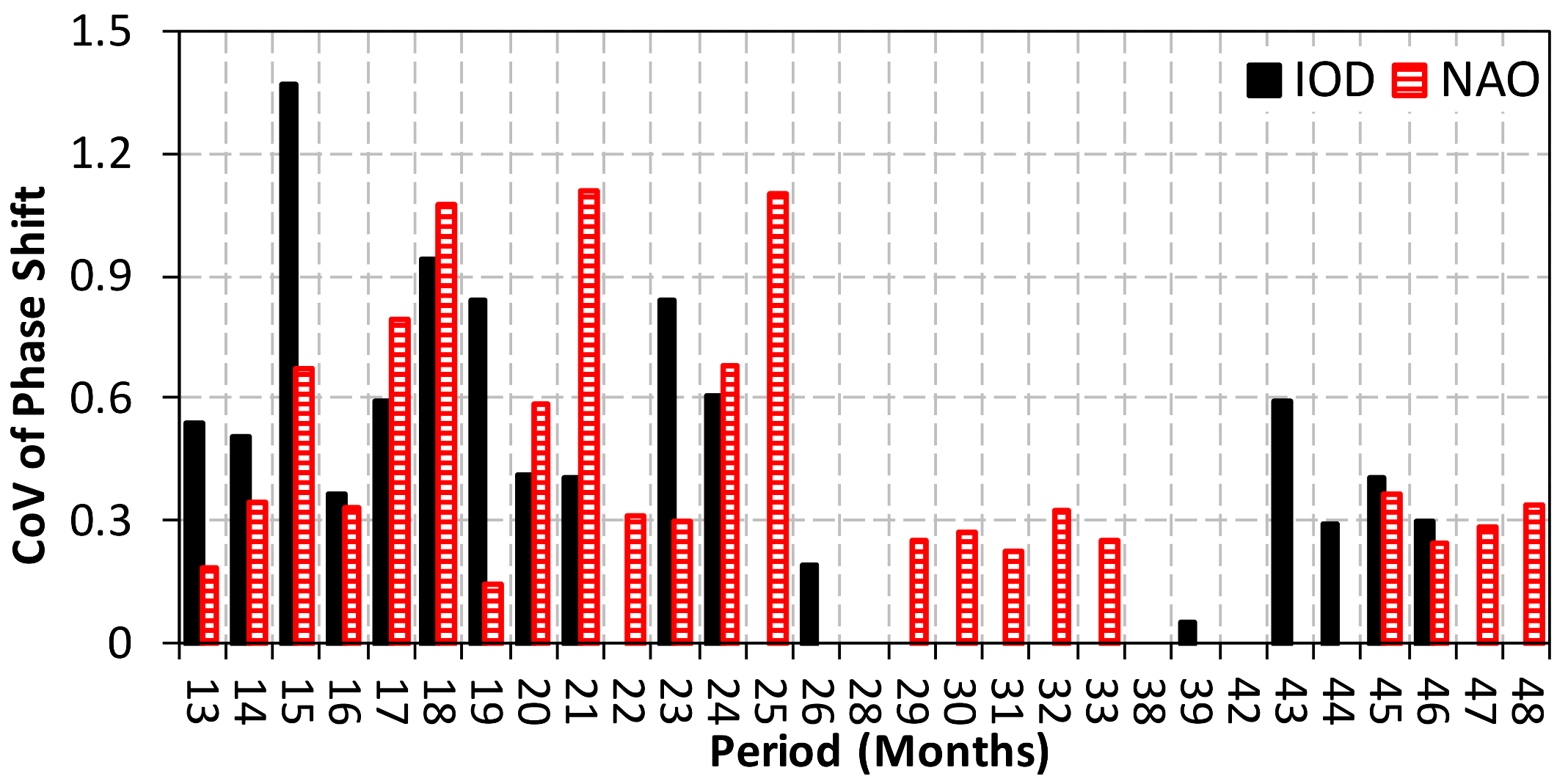
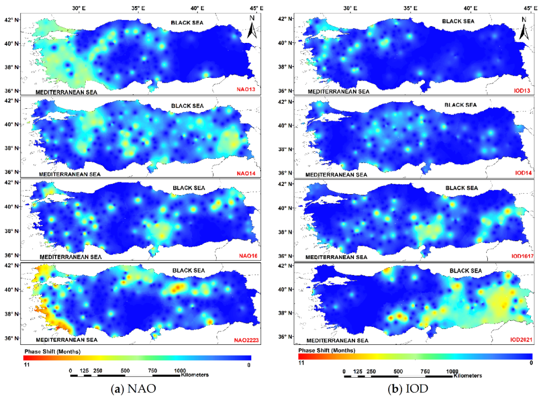
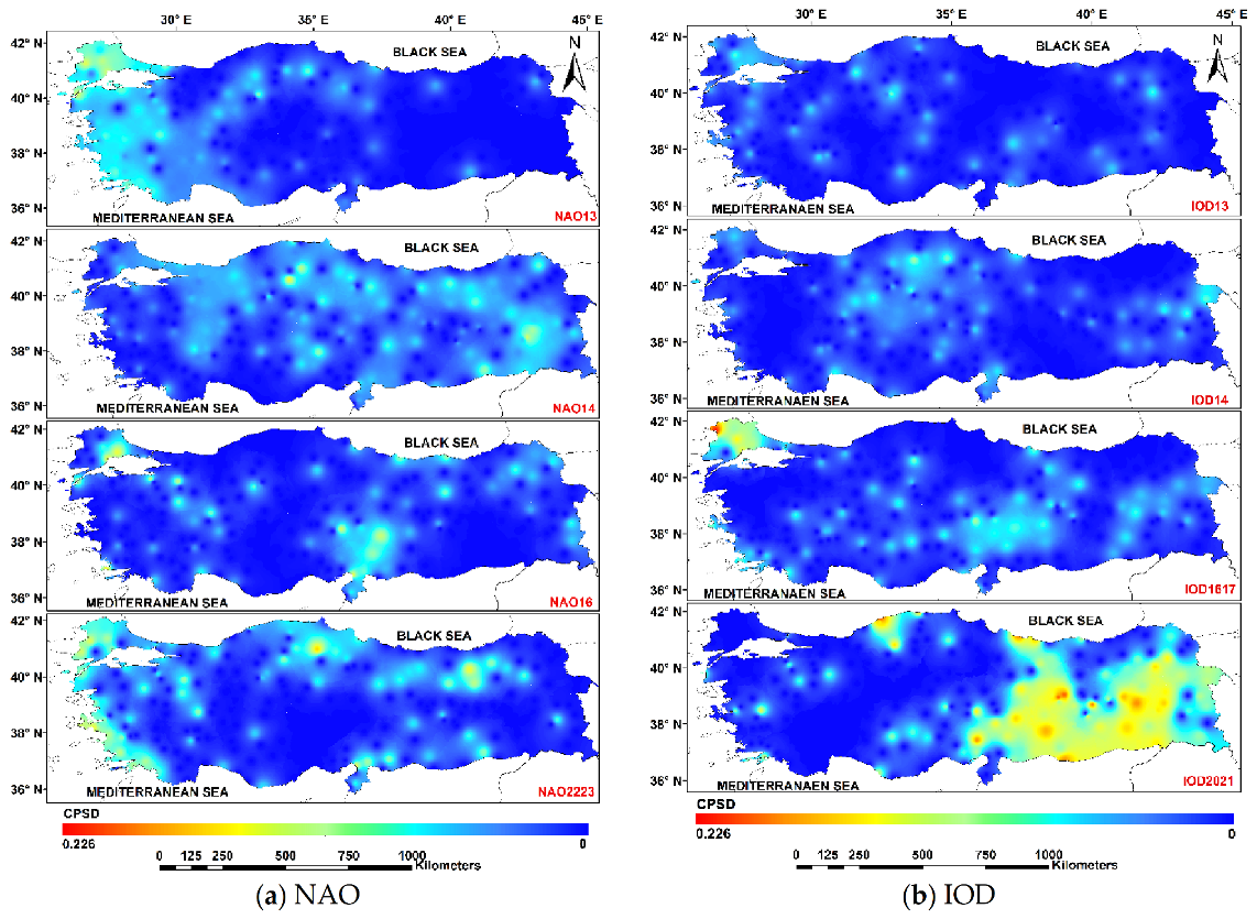
- According to the cross-spectral analysis results, phase shift and CPSD values between the NAO and meteorology stations were mostly clustered in the west of Turkey for the 22–23-month period. This means that the stronger relationships were observed in the west because the NAO is closer to west of Turkey. Similarly, phase shift and CPSD values between the IOD and meteorology stations were clustered for the 20–21-month period in the east and southeast of Turkey. Accordingly, the stronger relationships were observed in the east because the IOD is closer to east of Turkey. Therefore, Bodrum meteorology station in the west and Igdir meteorology station in the east were examined as examples in this study according to the strong relationships with the NAO and the IOD indices, respectively, for the above periods. Moreover, NAO2223 and IOD2021 showed strong relationships with western and eastern meteorology stations, respectively, in close periods (20–21 months and 22–23 months);
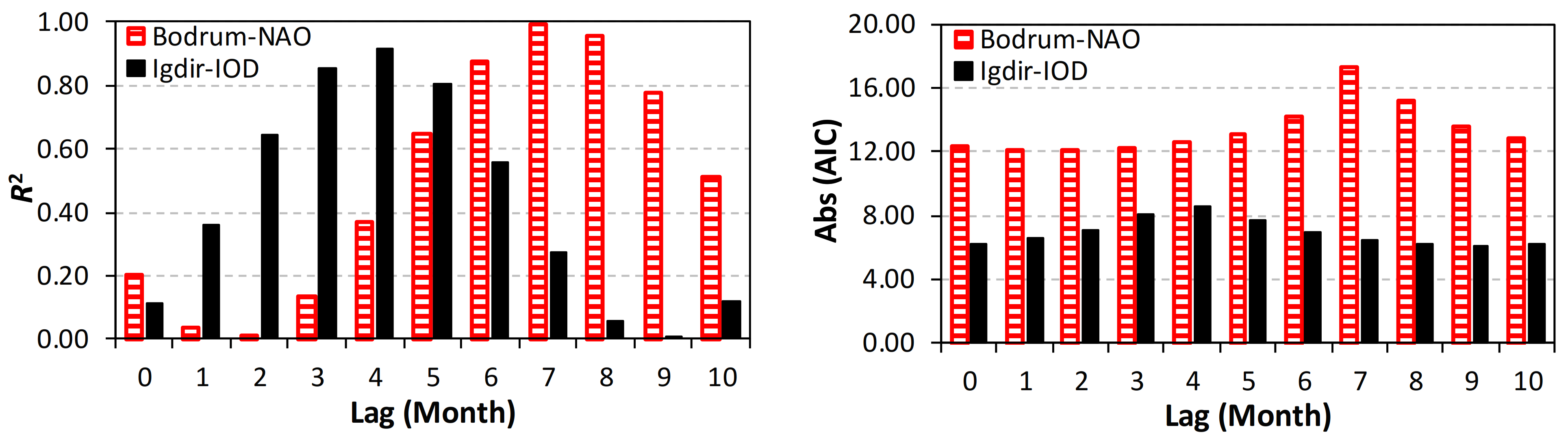
- The phase shift was calculated as 7.67 months for Bodrum-NAO in the 22-month period and as 4.33 months for Igdir-IOD in the 20-month period by cross-spectral analysis. These results indicate that the effect of the NAO is seen after 7.67 months in Bodrum meteorology station precipitation data and the effect of the IOD is seen after 4.33 months in Igdir meteorology station precipitation data. According to different phase shift values, the R2 and AIC values were obtained. Higher R2 and lower AIC values indicate a strong relationship between dependent and independent variables. After the linear modeling undertaken to statistically check the accuracy of the above values, the highest R2 (0.994 for Bodrum-NAO, 0.918 for Igdir-IOD) and lowest AIC (−17.240 for Bodrum-NAO, −8.596 for Igdir-IOD) values of the model were obtained at the 7-month phase shift point for Bodrum-NAO and at the 4-month phase shift point for Igdir-IOD. Thus, the phase shift values obtained for relevant period after the cross-spectral analysis were statistically verified;
- The NAO and the IOD indices can be used in precipitation forecast studies in western and eastern Turkey, respectively.
Author Contributions
Funding
Institutional Review Board Statement
Informed Consent Statement
Data Availability Statement
Acknowledgments
Conflicts of Interest
References
- Durkee, J.D.; Frye, J.D.; Fuhrmann, C.M.; Lacke, M.C.; Jeong, H.G.; Mote, T.L. Effects of the North Atlantic Oscillation on precipitation-type frequency and distribution in the eastern United States. Theor. Appl. Climatol. 2008, 94, 51–65. [Google Scholar] [CrossRef]
- Hurrell, J.W. North Atlantic climate variability: The role of the North Atlantic Oscillation. J. Mar. Syst. 2010, 79, 231–244. [Google Scholar] [CrossRef]
- Walker, G.T. Correlation in seasonal variations of weather IX: A further study of world weather. Mem. India Met. Dept. 1924, 24, 275–332. [Google Scholar]
- Walker, G.T.; Bliss, E.W. Memoirs of the Royal Meteorological Society. Q. J. R. Meteorol. Soc. 1932, 4, 53–84. [Google Scholar]
- Wallace, J.M. North Atlantic Oscillation/annular mode: Two paradigms one phenomenon. Q. J. R. Meteorol. Soc. 2000, 126, 791–805. [Google Scholar] [CrossRef]
- Hurrell, J.W. Decadal trends in the North Atlantic Oscillation, regional temperatures and precipitation. Science 1995, 269, 676–679. [Google Scholar]
- Hurrell, J.W.; Kushnir, Y.; Visbeck, M.; Ottersen, G. An overview of the North Atlantic Oscillation. Geophys. Monogr. 2003, 134, 1–35. [Google Scholar] [CrossRef] [Green Version]
- Wibig, J. Precipitation in Europe in relation to circulation patterns at the 500 hPa level. Int. J. Climatol. 1999, 19, 253–269. [Google Scholar] [CrossRef]
- Tatlı, H.; Menteş, Ş.S. Detrended cross-correlation patterns between North Atlantic oscillation and precipitation. Theor. Appl. Climatol. 2019, 138, 387–397. [Google Scholar] [CrossRef]
- Hurrell, J.W.; Van, L.H. Decadal variations in climate associated with the North Atlantic oscillation. Clim. Chang. 1997, 36, 301–326. [Google Scholar] [CrossRef]
- Vergni, L.; Lena, B.D.; Chiaudani, A. Statistical characterization of winter precipitation in the Abruzzo region (Italy) in relation to the North Atlantic Oscillation (NAO). Atmos. Res. 2016, 178–179, 279–290. [Google Scholar] [CrossRef]
- Zamrane, Z.; Turki, I.; Laignel, B.; Mahé, G.; Laftouhi, N.E. Characterization of the interannual variability of precipitation and streamflow in Tensift and Ksob basins (Morocco) and links with the NAO. Atmosphere 2016, 7, 84. [Google Scholar] [CrossRef] [Green Version]
- Castro, A.; Vidal, M.I.; Calvo, A.I.; Fernández, R.M.; Fraile, R. May the NAO index be used to forecast rain in Spain? Atmosfera 2011, 24, 251–265. [Google Scholar]
- Garcia, N.O.; Gimeno, L.; Torre, D.L.L.; Nieto, R.; Añel, J.A. North Atlantic Oscillation (NAO) and precipitation in Galicia (Spain). Atmosfera 2005, 18, 25–32. [Google Scholar]
- Massei, N.; Durand, A.; Deloffre, J.; Dupont, J.P.; Valdes, D.; Laignel, B. Investigating possible links between the North Atlantic Oscillation and precipitation variability in Northwestern France over the past 35 years. J. Geophys. Res. 2007, 112, D09121. [Google Scholar] [CrossRef] [Green Version]
- Hermida, L.; López, L.; Merino, A.; Berthet, C.; García, O.E.; Sánchez, J.L.; Dessens, J. Hailfall in southwest France: Relationship with precipitation, trends and wavelet analysis. Atmos. Res. 2015, 156, 174–188. [Google Scholar] [CrossRef]
- Saunders, M.A.; Qian, B. Seasonal predictability of the winter NAO from North Atlantic sea surface temperatures. Geophys. Res. Lett. 2002, 29, 1–6. [Google Scholar] [CrossRef] [Green Version]
- Eshel, G. Forecasting the North Atlantic Oscillation using North Pacific surface pressure. Mon. Weather Rev. 2003, 131, 1018–1025. [Google Scholar] [CrossRef]
- Wang, L.; Ting, M.; Kushner, P.J. A robust empirical seasonal prediction of winter NAO and surface climate. Sci. Rep. 2017, 7, 279. [Google Scholar] [CrossRef] [Green Version]
- Dobrynin, M.; Domeisen, D.I.V.; Müller, W.A.; Bell, L.; Brune, S.; Bunzel, F.; Düsterhus, A.; Fröhlich, K.; Pohlmann, H.; Baehr, J. Improved teleconnection based dynamical seasonal predictions of boreal winter. Geophys. Res. Lett. 2018, 45, 3605–3614. [Google Scholar] [CrossRef] [Green Version]
- Chlaściak, Ś.M.; Niedzielski, T. Forecasting the North Atlantic Oscillation index using altimetric sea level anomalies. Acta Geod. Geophys. 2020, 55, 531–553. [Google Scholar] [CrossRef]
- Saji, N.H.; Goswami, B.N.; Vinayachandran, P.N.; Yamagata, T. A dipole mode in the tropical Indian Ocean. Nature 1999, 401, 360–363. [Google Scholar] [CrossRef] [PubMed]
- Saji, N.H.; Yamagata, T. Possible impacts of Indian Ocean Dipole mode events on global climate. Clim. Res. 2003, 25, 151–169. [Google Scholar] [CrossRef]
- Clark, C.O.; Webster, P.J.; Cole, J.E. Interdecadal variability of the relationship between the Indian Ocean zonal mode and East African coastal rainfall anomalies. J. Clim. 2003, 16, 548–554. [Google Scholar] [CrossRef] [Green Version]
- Dubache, G.; Ogwang, B.A.; Ongoma, V.; Islam, A.R.M.T. The effect of Indian Ocean on Ethiopian seasonal rainfall. Meteorol. Atmos. Phys. 2019, 131, 1753–1761. [Google Scholar] [CrossRef]
- Guan, Z.; Ashok, K.; Yamagata, T. Summertime response of the tropical atmosphere to the Indian Ocean sea surface temperature anomalies. J. Meteorol. Soc. Jpn. 2003, 81, 533–561. [Google Scholar] [CrossRef] [Green Version]
- Yuan, Y.; Yang, H.; Zhouc, W.; Li, C. Influences of the Indian Ocean dipole on the Asian summer monsoon in the following year. Int. J. Climatol. 2008, 28, 1849–1859. [Google Scholar] [CrossRef]
- Hussain, M.S.; Kim, S.; Lee, S. On the relationship between Indian Ocean Dipole events and the precipitation of Pakistan. Theor. Appl. Climatol. 2016, 130, 673–685. [Google Scholar] [CrossRef]
- Saji, N.H.; Ambrizzi, T.; Ferraz, S.E.T. Indian Ocean Dipole mode events and austral surface air temperature anomalies. Dyn. Atmos. Ocean. 2005, 39, 87–101. [Google Scholar] [CrossRef]
- Hardiman, S.C.; Dunstone, N.J.; Scaife, A.A.; Smith, D.M.; Knight, J.R.; Davies, P.; Claus, M.; Greatbatch, R.J. Predictability of European winter 2019/20: Indian Ocean dipole impacts on the NAO. Atmos. Sci. Lett. 2020, 1–10. [Google Scholar] [CrossRef]
- Chan, S.C.; Behera, S.K.; Yamagata, T. Indian Ocean Dipole influence on South American rainfall. Geophys. Res. Lett. 2008, 35, L14S12. [Google Scholar] [CrossRef]
- Sariş, F.; Hannah, D.M.; Eastwood, W.J. Spatial variability of precipitation regimes over Turkey. Hydrol. Sci. J. 2010, 55, 234–249. [Google Scholar] [CrossRef] [Green Version]
- Türkeş, M.; Erlat, E. Climatological responses of winter precipitation in Turkey to variability of the North Atlantic Oscillation during the period 1930–2001. Theor. Appl. Climatol. 2005, 81, 45–69. [Google Scholar] [CrossRef]
- Türkeş, M.; Erlat, E. Precipitation changes and variability in Turkey linked to the north atlantic oscillation during the period 1930–2000. Int. J. Climatol. 2003, 23, 1771–1796. [Google Scholar] [CrossRef]
- Türkeş, M.; Erlat, E. Winter mean temperature variability in Turkey associated with the North Atlantic Oscillation. Meteorol. Atmos. Phys. 2009, 105, 211–225. [Google Scholar] [CrossRef]
- Küçük, M.; Kahya, E.; Cengiz, T.M.; Karaca, M. North Atlantic Oscillation influences on Turkish lake levels. Hydrol. Process 2009, 23, 893–906. [Google Scholar] [CrossRef]
- Kahya, E. The Impacts of NAO on the hydrology of the Eastern Mediterranean. Adv. Glob. Chang. Res. 2011, 46, 57–71. [Google Scholar] [CrossRef]
- Bozyurt, O.; Özdemir, M.A. The relations between North Atlantic Oscillation and minimum temperature in Turkey. Procedia Soc. Behav. Sci. 2014, 120, 532–537. [Google Scholar] [CrossRef] [Green Version]
- Sönmez, İ.; Kömüşcü, A.Ü. Reclassification of rainfall regions of Turkey by K-means methodology and their temporal variability in relation to North Atlantic Oscillation (NAO) . Theor. Appl. Climatol. 2011, 106, 499–510. [Google Scholar] [CrossRef]
- Baltacı, H.; Akkoyunlu, B.O.; Tayanç, M. Relationships between teleconnection patterns and Turkish climatic extremes. Theor. Appl. Climatol. 2018, 134, 1365–1386. [Google Scholar] [CrossRef]
- Baltaci, H.; Arslan, H.; Akkoyunlu, B.O.; Gomes, H.B. Long-term variability and trends of extended winter snowfall in Turkey and the role of teleconnection patterns. Meteorol. Appl. 2020, 27, e1891. [Google Scholar] [CrossRef]
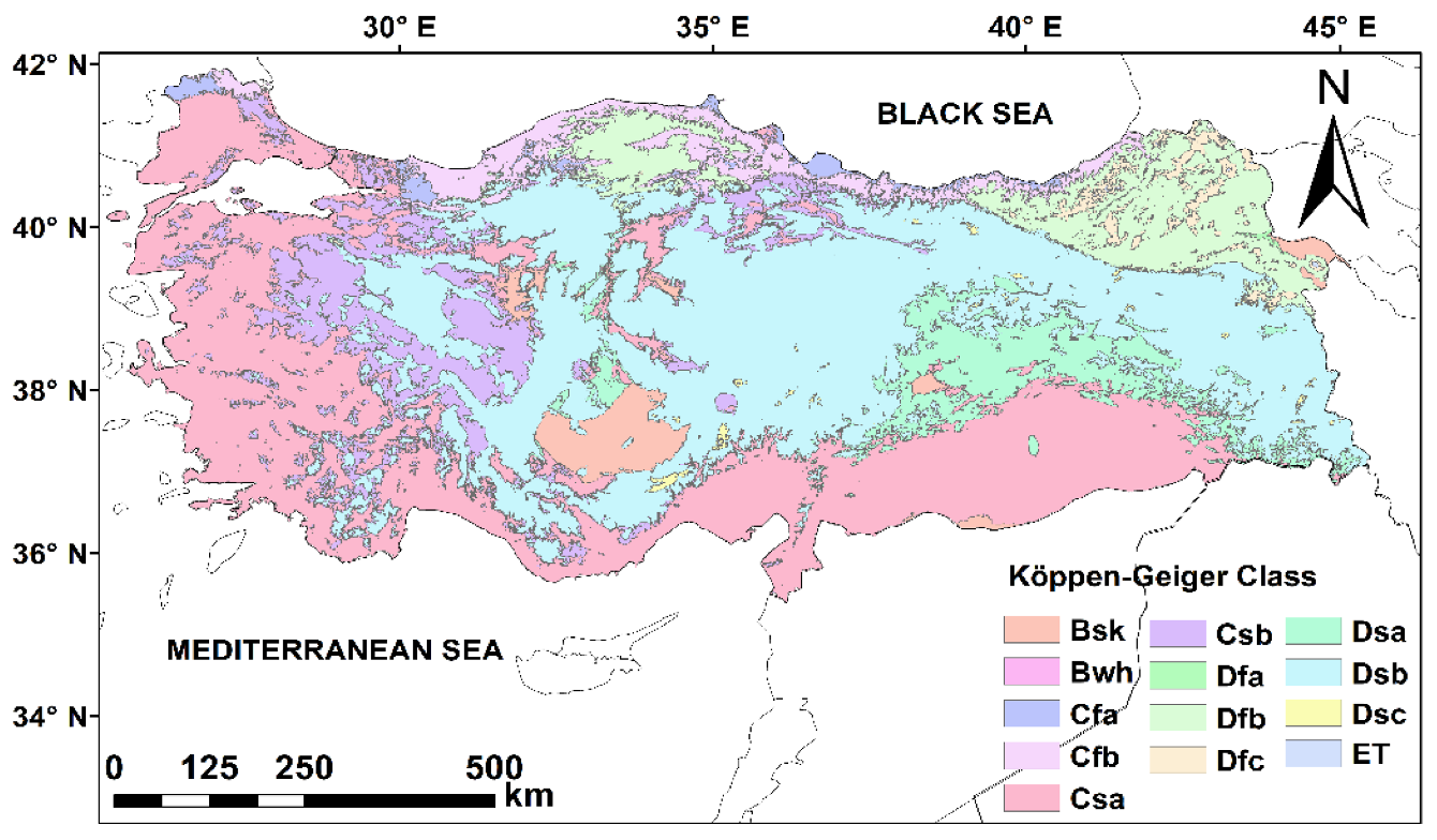
- Yılmaz, E.; Çiçek, İ. Detailed Köppen-Geiger climate regions of Turkey. Int. J. Hum. Sci. 2018, 15, 225–242. (In Turkish) [Google Scholar] [CrossRef] [Green Version]
- Jones, P.D.; Jonsson, T.; Wheeler, D. Extension to the North Atlantic Oscillation using early instrumental pressure observations from Gibraltar and south-west Iceland. Int. J. Climatol. 1997, 17, 1433–1450. [Google Scholar]
- ClimateDataGuide. Available online: https://climatedataguide.ucar.edu/climate-data/hurrell-north-atlantic-oscillation-theNAO-index-station-based.climatedataguide.ucar.edu (accessed on 12 September 2019).
- NOAA. Available online: https://psl.noaa.gov/gcos_wgsp/Timeseries/Data/dmi.long.data (accessed on 12 September 2019).
- Blackman, R.B.; Tukey, J.W. The Measurement of Power Spectra. Bell Syst. Tech. 1958, 37, 185. [Google Scholar] [CrossRef]
- Trauth, M.H. MATLAB Recipes for Earth Sciences Fourth Edition 2014; Springer: Berlin/Heidelberg, Germany, 2014. [Google Scholar]
- Kutzbach, J.E.; Bryson, R.A. Variance spectrum of Holocene climatic fluctuations in the north Atlantic sector. J. Atmos. Sci. 1974, 31, 1958–1963. [Google Scholar] [CrossRef]
- Allen, M.R. Interactions between the Atmosphere and Oceans on Time-Scales of Weeks to Years. Ph.D. Thesis, University of Oxford, Oxford, UK, 1992. [Google Scholar]
- Allen, M.R.; Smith, L.A. Investigating the Origins and Significance of Low-Frequency Modes of Climate Variability. Geophys. Res. Lett. 1994, 21, 883–886. [Google Scholar] [CrossRef]
- Gilman, D.L.; Fuglister, F.J.; Mitchell, J.M., Jr. On the Power Spectrum of “Red Noise”. J. Atmos. Sci. 1963, 20, 182–184. [Google Scholar]
- Mann, M.E.; Lees, J.M. Robust estimation of background noise and signal detection in climatic time series. Clim. Chang. 1996, 33, 409–445. [Google Scholar] [CrossRef]
- Matyasovszky, I. Estimating red noise spectra of climatological time series. Idoejaras 2013, 117, 187–200. [Google Scholar]
- Ghil, M.; Allen, M.R.; Dettinger, M.D.; Ide, K.; Kondrashov, D.; Mann, M.E.; Robertson, A.W.; Saunders, A.; Tian, Y.; Varadi, F.; et al. Advanced spectral methods for climatic time series. Rev. Geophys. 2002, 40, 1–41. [Google Scholar] [CrossRef] [Green Version]
- Dickey, D.A.; Fuller, W.A. Distribution of the estimators for autoregressive time series with a unit root. J. Am. Stat. Assoc. 1979, 74, 427–431. [Google Scholar] [CrossRef]


| Bodrum-NAO | Igdir-IOD | ||||||||
|---|---|---|---|---|---|---|---|---|---|
| Peak Num | Frequency | Period | CPSD | Phase Shift | Peak Num | Frequency | Period | CPSD | Phase Shift |
| P1 | 0.039551 | 25 | 0.086702 | 6 | P1 | 0.043457 | 23 | 0.117002 | −5 |
| P2 | 0.044922 | 22 | 0.087209 | −8 | P2 | 0.049805 | 20 | 0.116221 | −4 |
| P3 | 0.060059 | 17 | 0.053597 | 3 | P3 | 0.053223 | 19 | 0.076957 | 1 |
| P4 | 0.064453 | 16 | 0.143938 | −7 | P4 | 0.056152 | 18 | 0.136801 | 3 |
| P5 | 0.073242 | 14 | 0.045073 | −6 | P5 | 0.060059 | 17 | 0.058649 | −5 |
| P6 | 0.077637 | 13 | 0.078003 | −5 | P6 | 0.066406 | 15 | 0.046864 | 2 |
| P7 | 0.069336 | 14 | 0.074182 | −3 | |||||
| P8 | 0.073730 | 14 | 0.042564 | 4 | |||||
| Bodrum-NAO | Igdir-IOD | ||||||||
|---|---|---|---|---|---|---|---|---|---|
| Peak Num | Frequency | Period | CPSD | Phase Shift | Peak Num | Frequency | Period | CPSD | Phase Shift |
| P1 | 0.039551 | 25 | 0.096240 | 5 | P1 | 0.043457 | 23 | 0.119168 | −6 |
| P2 | 0.044922 | 22 | 0.048841 | −7 | P2 | 0.049805 | 20 | 0.134552 | −5 |
| P3 | 0.060059 | 17 | 0.043726 | 6 | P3 | 0.053223 | 19 | 0.109736 | 3 |
| P4 | 0.063965 | 16 | 0.090910 | 7 | P4 | 0.056641 | 18 | 0.120374 | 4 |
| P5 | 0.073242 | 14 | 0.033206 | 6 | P5 | 0.05957 | 17 | 0.077557 | −4 |
| P6 | 0.077637 | 13 | 0.072500 | −4 | P6 | 0.066406 | 15 | 0.093127 | 3 |
| P7 | 0.069336 | 14 | 0.084341 | −3 | |||||
| P8 | 0.073730 | 14 | 0.057047 | 4 | |||||
| Bodrum-NAO | Igdir-IOD | |||
|---|---|---|---|---|
| Phase Shift (Months) | R2 | AIC | R2 | AIC |
| 0 | 0.204 | −12.323 | 0.114 | −6.223 |
| 1 | 0.035 | −12.130 | 0.360 | −6.547 |
| 2 | 0.009 | −12.103 | 0.644 | −7.132 |
| 3 | 0.133 | −12.237 | 0.857 | −8.045 |
| 4 | 0.369 | −12.557 | 0.918 | −8.596 |
| 5 | 0.646 | −13.137 | 0.802 | −7.719 |
| 6 | 0.879 | −14.208 | 0.555 | −6.908 |
| 7 | 0.994 | −17.240 | 0.271 | −6.414 |
| 8 | 0.957 | −15.246 | 0.060 | −6.158 |
| 9 | 0.778 | −13.608 | 0.003 | −6.097 |
| 10 | 0.514 | −12.822 | 0.120 | −6.220 |
Publisher’s Note: MDPI stays neutral with regard to jurisdictional claims in published maps and institutional affiliations. |
© 2021 by the authors. Licensee MDPI, Basel, Switzerland. This article is an open access article distributed under the terms and conditions of the Creative Commons Attribution (CC BY) license (http://creativecommons.org/licenses/by/4.0/).
Share and Cite
Demir, U.S.; Koc, A.C. Investigation of the North Atlantic Oscillation and Indian Ocean Dipole Influence on Precipitation in Turkey with Cross-Spectral Analysis. Atmosphere 2021, 12, 99. https://0-doi-org.brum.beds.ac.uk/10.3390/atmos12010099
Demir US, Koc AC. Investigation of the North Atlantic Oscillation and Indian Ocean Dipole Influence on Precipitation in Turkey with Cross-Spectral Analysis. Atmosphere. 2021; 12(1):99. https://0-doi-org.brum.beds.ac.uk/10.3390/atmos12010099
Chicago/Turabian StyleDemir, Umut Sakine, and Abdullah Cem Koc. 2021. "Investigation of the North Atlantic Oscillation and Indian Ocean Dipole Influence on Precipitation in Turkey with Cross-Spectral Analysis" Atmosphere 12, no. 1: 99. https://0-doi-org.brum.beds.ac.uk/10.3390/atmos12010099