
A GPU-Accelerated Radiation Transfer Model Using the Lattice Boltzmann Method

1
DEVCOM Army Research Laboratory, Adelphi, MD 20783, USA
2
US Navy Research Laboratory, Washington, DC 20375, USA
*
Author to whom correspondence should be addressed.
Atmosphere 2021, 12(10), 1316; https://0-doi-org.brum.beds.ac.uk/10.3390/atmos12101316
Submission received: 4 August 2021
/
Revised: 22 September 2021
/
Accepted: 28 September 2021
/
Published: 9 October 2021
(This article belongs to the Section Atmospheric Techniques, Instruments, and Modeling)
Abstract
:A prototype of a three-dimensional (3-D) radiation model is developed using the lattice Boltzmann method (LBM) and implemented on a graphical processing unit (GPU) to accelerate the model’s computational speed. This radiative transfer-lattice Boltzmann model (RT-LBM) results from a discretization of the radiative transfer equation in time, space, and solid angle. The collision and streaming computation algorithm, widely used in LBM for fluid flow modeling, is applied to speed up the RT-LBM computation on the GPU platform. The isotropic scattering is assumed in this study. The accuracy is evaluated using Monte Carlo method (MCM) simulations, showing RT-LBM is quite accurate when typical atmospheric coefficients of scattering and absorption are used. RT-LBM runs about 10 times faster than the MCM in a same CPU. When implemented on a NVidia Tesla V100 GPU in simulation with a large number of computation grid points, for example, RT-LBM runs ~120 times faster than running on a single CPU. The test results indicate RT-LBM is an accurate and fast model and is viable for simulating radiative transfer in the atmosphere with ranges for the isotropic atmosphere radiative parameters of albedo scattering (0.1~0.9) and optical depth (0.1~12).
1. Introduction
Radiative energy transfer plays an important role in many areas of science and technology. Accurate modeling of incoming solar radiation and outgoing infrared radiation from the Earth’s surface and their interactions with atmospheric constituents has been among the most important tasks for the atmospheric sciences and remote sensing of environments. Compared with cloud-free and large-scale atmospherics, in which radiative transfer is usually treated one-dimensionally by assuming horizontal homogeneity, radiation transfer near the ground is a complex three-dimensional (3-D) phenomenon due to interactions with the Earth’s surface features, such as terrains, buildings, soil, and vegetation. The mathematical description of electromagnetic radiation propagation is the radiative transfer equation (RTE) with associated emission, absorption, and scattering parameters and complex boundary conditions. Analytical solutions for real atmospheric conditions are not available. Due to the complexity and difficulties in solving the RTE, many numerical methods, such as the Monte Carlo method (MCM) [1], finite volume method (FVM) [2], and discrete ordinates method (DOM) [3], to name a few, have been developed. Proper choice of numerical method is dependent on the problem parameters and boundary conditions. The MCM is considered as a versatile and accurate method that can handle complex situations and is free from numerical errors such as ray effects, numerical smearing, and false scattering [1,3,4]. Therefore, the MCM is often used as a benchmark tool for radiative transfer modeling. The drawback with the MCM is it requires a very large number of photons to be released to avoid statistical noise; therefore, it is computationally expensive. FVM and DOM have the advantages of ease and efficiency to set up the radiative transfer problem but have the problems of ray effects and slow convergence in small optical thickness situations. All the above numerical methods for solving the RTE demand a great deal of computation power for a large computational domain. Moreover, variations of scattering and absorption coefficients depend on atmosphere constituents in different wavelengths, which require multiple computations for different wavelengths, thus making the computation load even more formidable.
In recent years, a novel and powerful method, the lattice Boltzmann method (LBM), has been developed for solving the RTE. One of the motives for using the LBM in solving the RTE is to improve the computation speed of radiative transfer modeling. The LBM was first discovered and developed in the fluid mechanics community [5,6,7,8,9,10,11] and has become one of the most effective methods for fluid flow and heat transfer simulations. The LBM is based on the kinetic theory of statistical mechanics and solves the Boltzmann equation that governs the probability distribution of fluid particles. The LBM solves the Boltzmann equation for a particle at each grid point by performing collision and propagation calculations of the particle’s probability distribution function (PDF) over a discrete and symmetric lattice mesh with certain fixed directions. The macroscopic variables, such as fluid density and velocity, are computed from the statistical moments of the particle PDF. The major advantages of the LBM in fluid modeling are its intrinsic parallelism and the ease with which it treats complex boundary conditions. Flow modeling using the LBM is as accurate as FV or finite elements (FE) methods, and has a computation speed several hundred times faster than FV and FE methods.
It is natural to explore the LBM as a computational method to accelerate the computation speed in solving the RTE because radiative transfer is one of most computationally intensive tasks in atmospheric modeling. The LBM can be considered a direct discretization of the Boltzmann equation [7]. The earliest work of solving the RTE using the LBM by Geist et al. [12] was to investigate lighting in computer graphics with angular discretization with 19 directions and using a graphics processing unit (GPU) for computation [13]. Because of the similarity between the RTE and Boltzmann equation [14], earlier research and development of the LBM for the RTE started with direct discretization of the RTE with respect of space, time, and angular direction, which is a valid approach [7,14]. Asinari et al. and Mishra et al. [15,16] developed a two-dimensional (2-D) LBM for radiative transfer modeling in a particular medium. Ma et al. [17] derived an LBM used for a one-dimensional (1-D) radiation problem that compared well with an analytical solution. Bindra and Patil [18] and McCulloch and Bindra [19] also developed a 2-D LBM for the RTE for a simulation of the conjugated radiative and convective heat transfer problem. A general review on modeling neutron and photon transport using LBM is provided in [20]. The LBM was also used in a non-equilibrium radiation transfer problem [21]. Zhang et al. [22] and Yi et al. [23] derived a 2-D LBM using the Chapman–Enskog expansion for a steady-state radiative transfer problem that can deal with both thin and high optical depths. The LBM was used in a model for astronomical radiation transfer by Weih et al. [24]. For a better treatment of the radiation source term, a multi-relaxation time LBM was developed by Liu et al. [25]. McHardy et al. [26,27] developed a 3-D LBM model using a direct discretization of the RTE and the model produced accurate results for the ballistic radiation condition in which the medium scattering albedo is less than 0.7. An anisotropic case of Mie scattering was also computed and compared well with the LBM method [26]. Mink et al. [28,29] developed a 3-D LBM method for high optical thickness situations based on the Chapman–Enskog expansion and a steady-state RTE was approximated by the Helmholtz equation and solved with the LBM.
The LBM with a GPU has shown to be very effective in numerical simulation of turbulent flow in urban environments with at least a 200 to 500 times speed-up (CPU/GPU time ratio) depending on the GPU type [30,31]. Since radiative transfer is a very important component of energy transfer in the atmospheric boundary layer and the computation is very challenging, it is advantageous to exploit the LBM method with a GPU when solving the RTE. It is also beneficial to have the same computational methodology and grids set up for coupling our LBM flow model and the LBM radiative transfer model.
The objective of this study is to evaluate the accuracy and computation capability in a newly developed radiative transfer model using the lattice Boltzmann method, called RT-LBM. Specifically, we focus on RT-LBM’s accuracy in simulating direct solar radiation with different incoming boundary conditions. The computation speeds using a GPU and a CPU are compared for different sizes of computational grid setups. The organization of this work is as follows: The second section describes the derivation of RT-LBM, radiation parameters, boundary conditions, and its computation method. The Monte Carlo (MC) radiative transfer model used for the comparison study is also described in this section. The third section presents the results of RT-LBM simulations of radiative transfer around buildings and compares the model results using the well-established MCM. The computation speeds of RT-LBM on a GPU are described and compared with CPU implementation. The final section gives a summary and discussion of applications of RT-LBM.
2. Methods
2.1. The Lattice Boltzmann Model for Radiative Transfer
Spectral radiance propagation in a scattering and absorbing medium is described by the following RTE:
where is the radiance at spatial point x and time t that travels along unit vector n into the solid angle with the speed of light c. are the absorption and scattering coefficients of the medium, respectively; is the blackbody radiance of the medium; and is the scattering phase function of the medium. S is other radiation source such as radiation from ground, road, and buildings in the atmospheric boundary layer. This term is epically important in the atmospheric boundary layer. It is also a very complex term which deserved a very careful and thorough study. Since this paper is focused on the solar radiation transfer, we neglected the source term hereafter in this paper. The integral term represents the radiation scattered from the other directions onto the volume surface. The spectral dependence is omitted since a participating medium with a specific wavelength band is considered in this paper.
According to a kinetic theory of radiative transport [14], the RTE can be written as the Boltzmann equation form using a probability distribution function (PDF), f of a virtual radiative particle or a photon [26,29]. The relation between the PDF at a direction i ( of a virtual particle or photon and the radiance is expressed as
where are the weights corresponding to the lattice directions (Figure 1). Neglecting the medium blackbody radiation source term for a much smaller magnitude in a clear atmospheric boundary layer, the RTE of Equation (1) can be written in following form:
where c is the speed of light and in the finite directions. The Boltzmann form of the RTE can be discretized in space in specific lattice directions, i (Figure 1), and time, t, as follows [7,26]:
The time step is related to the lattice length and , With the above definitions, the macroscopic radiation quantities, I (radiative intensity) and J (radiation flux vector), are computed from the statistical moments of the particle PDF, f,
which are resulted from following integral form equations providing the (2) as the connection.
It is important to point out that the equilibrium function in the collision term has a different mechanism in radiative transfer than in fluid flow. The in radiative transfer represents the interaction of photons with the surrounding medium rather than the equilibrium PDF of fluid particle collision in the LBM for fluid modeling. The is defined as follows:
where is the discrete scattering matrix describing the probability that a photon is scattered from the i to j direction, and are the weighting factors corresponding to the direction i. This function can be used for describing the anisotropic scattering by prescribing the elements of . For the isotropic scattering considered in this work, .
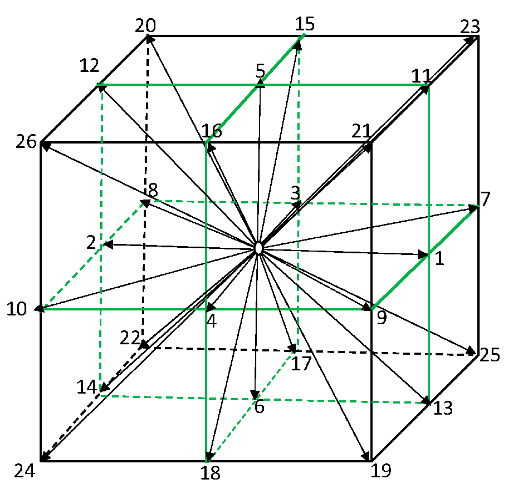
The computation domain is first divided into structured cubic grids. For each grid point (0 point in Figure 1), there are 26 lattice directions and neighbor points. The computational algorithm for RT-LBM takes typical collision and streaming operations for each time step. The collision operation is computed in the terms on the right hand of Equation (4), where the interactions, the scattering and absorption, of the photon with medium particles in every lattice direction are accounted for. The equilibrium PDF is computed as in Equation (9). In the streaming operation, the probability in a grid point is propagated in every direction to neighbor grid points (1 to 26) for the next time step. The macroscopic radiative variables are computed from Equations (5) and (6).
To keep the model non-dimensional for the comparisons and applications, the medium’s scattering albedo, a, and optical depth, b, (non-dimensional parameters) are used instead of the coefficients of absorption and scattering. The characteristic length scale for the photon is representing the length of a photon’s free path between two consecutive scattering events. The relationship between these parameters is expressed as
where = 1 is a modeled normalized physical domain length.
2.2. The Monte Carlo Model of Solar Radiation
A MC model is used to evaluate RT-LBM. It tracks a plentiful luminosity packet (referred to hereafter as MC “photons”) first and then counts them statistically for distribution of radiative intensity as a function of location, direction, and frequency. Each package carries energy L Δt/N, where N is the number of MC photons. As a result, each MC photon represents L Δt/(N hν) real photons, where hν denotes the energy of a real photon.
The MC model emits plentiful MC photons to mimic a radiation source. Each photon travels a distance s and then is scattered, absorbed, or re-emitted. The distance s is determined by
where ξ is a random number between 0 and 1. After traveling the distance s, the photon is scattered if a new random number, ξ, is below a; otherwise, the photon is absorbed.
The direction of scattering photon is described by the zenith angle θ and the azimuth angle ϕ. Since scattering is assumed to be isotropic in the model, θ and ϕ are chosen as [32]
ϕ = 2πξ
θ = 2πcos−1(2ξ − 1)
The MC model uses (10) and (11) to simulate solar radiation that penetrates the model top downward. It emits 5 × 10⁹ MC photons to mimic the incoming solar radiation and then tracks them in the atmosphere individually. Its statistical results are eventually used to obtain the distribution of radiative intensity.
2.3. The Computation Domains Setup and Boundary Conditions
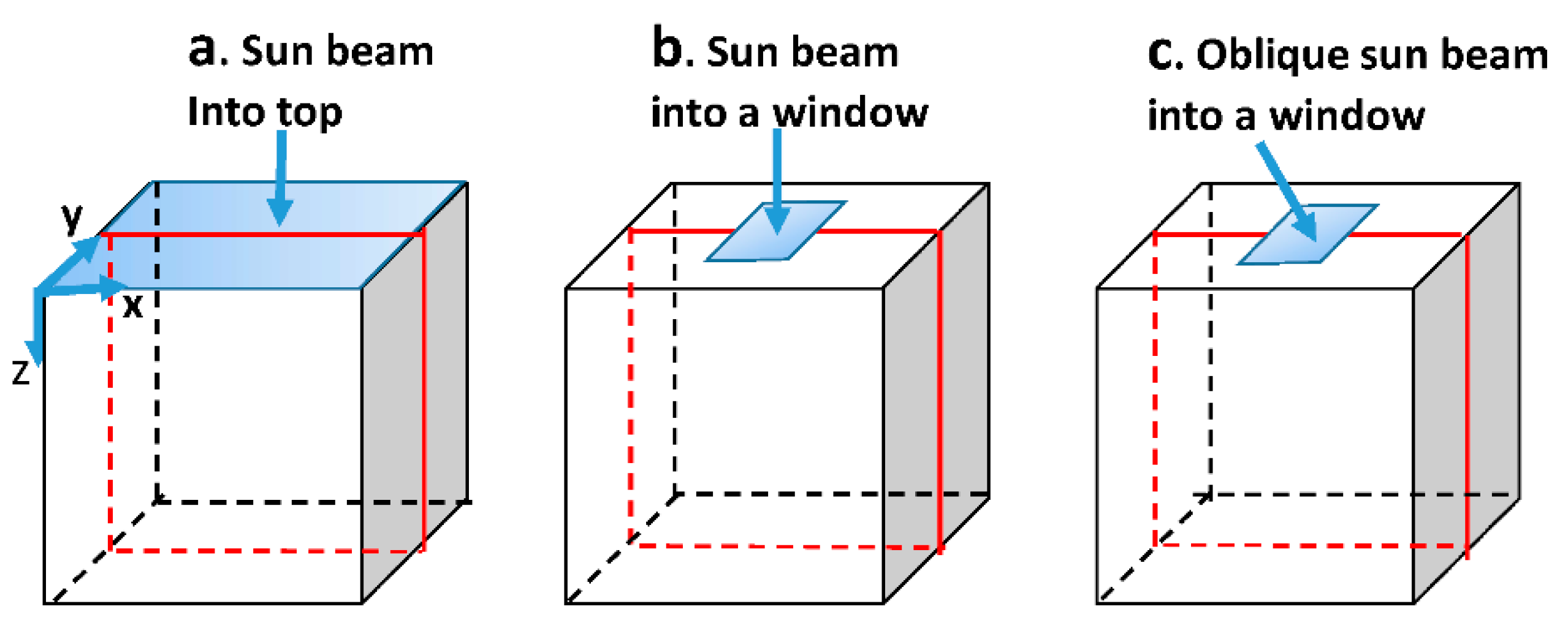
The design of the 3-D modeling domains is shown in Figure 2. All three cubic domains have the same number of computational grid points (101 × 101 × 101) in the x, y, and z directions. In the GPU computation speed test (Section 3.3), two setups of computational grid points were made much more dense, 501 × 501 × 201, to evaluate the effect of the number of grid points on computation speed.
All the incoming solar beam radiation is from the top boundary. The first is the incoming boundary which includes the entire top plane of the computational domain (Figure 2a), the second is the center window incoming boundary condition of the top boundary (Figure 2b), and the third (Figure 2c) is the window incoming boundary with oblique incoming direct solar radiation. A unit radiative intensity at the top surface is prescribed for direct solar radiation,
3. Results
RT-LBM is evaluated with the MC models, since high-density 3-D radiation field data for these kinds of simulation are not available for comparison. Although the MC model generally requires much more computation power, it has been proven to be a versatile and accurate method for modeling radiative transfer processes [1,26,29]. In the following validation cases, the same computation domain setups, boundary conditions, and radiative parameters were used in the RT-LBM and MC models. In these simulations, we set every variable as non-dimensional, including the unit length of the simulation domain in the x, y, and z directions. Normalized, non-dimensional results provide convenience for application of the simulation results. The model domain is a unit cube, with 101 × 101 × 101 grid points in these simulations except in Section 3.3. The top face of the cubic volume is prescribed with a unit of incoming radiation intensity. The rest of the boundary faces are black walls, i.e., there is no incoming radiation and outgoing radiation freely passes out of the lateral and bottom boundaries.
3.1. Direct Solar Beam Radiation Perpendicular to the Entire Top Boundary
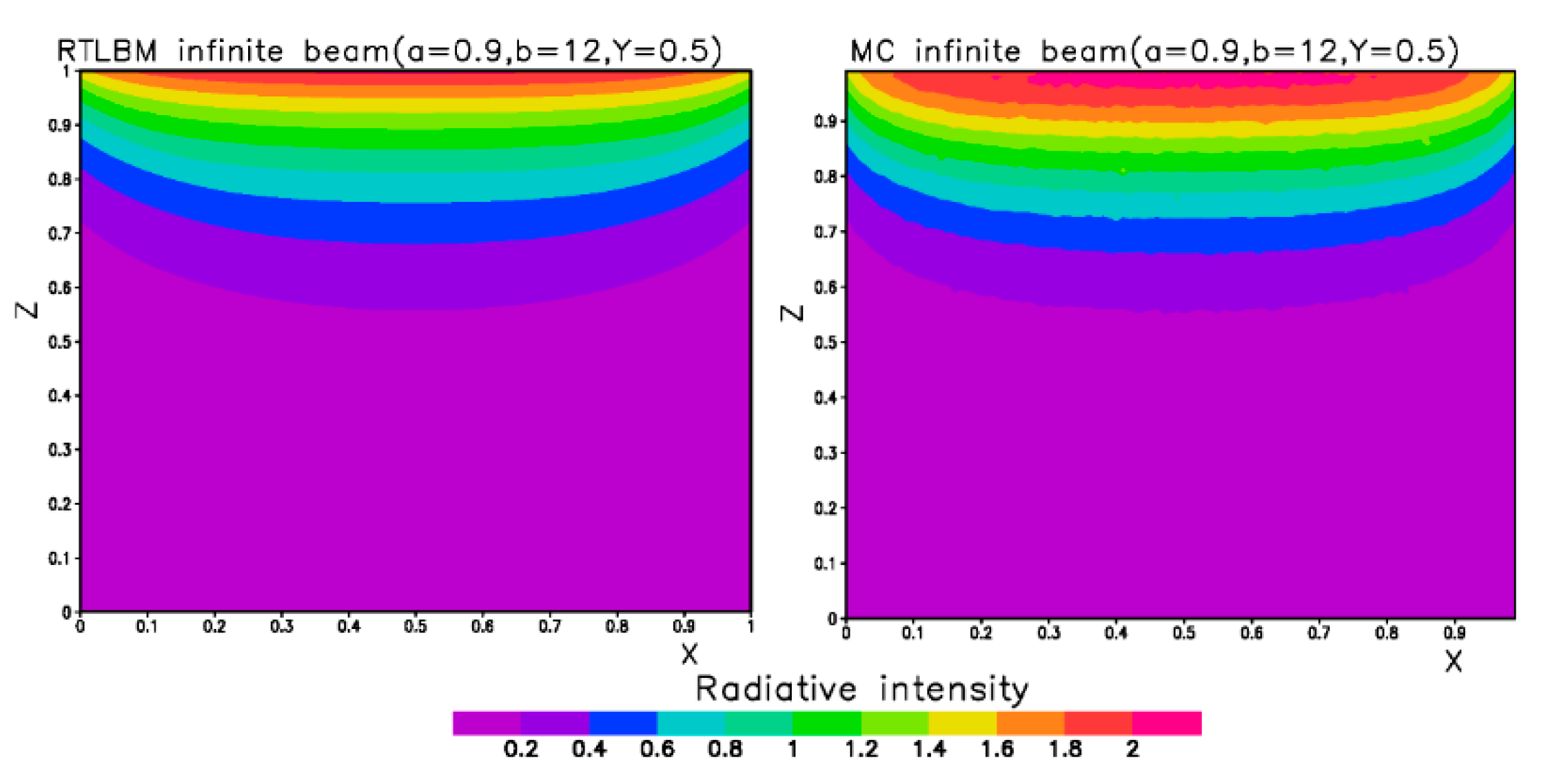
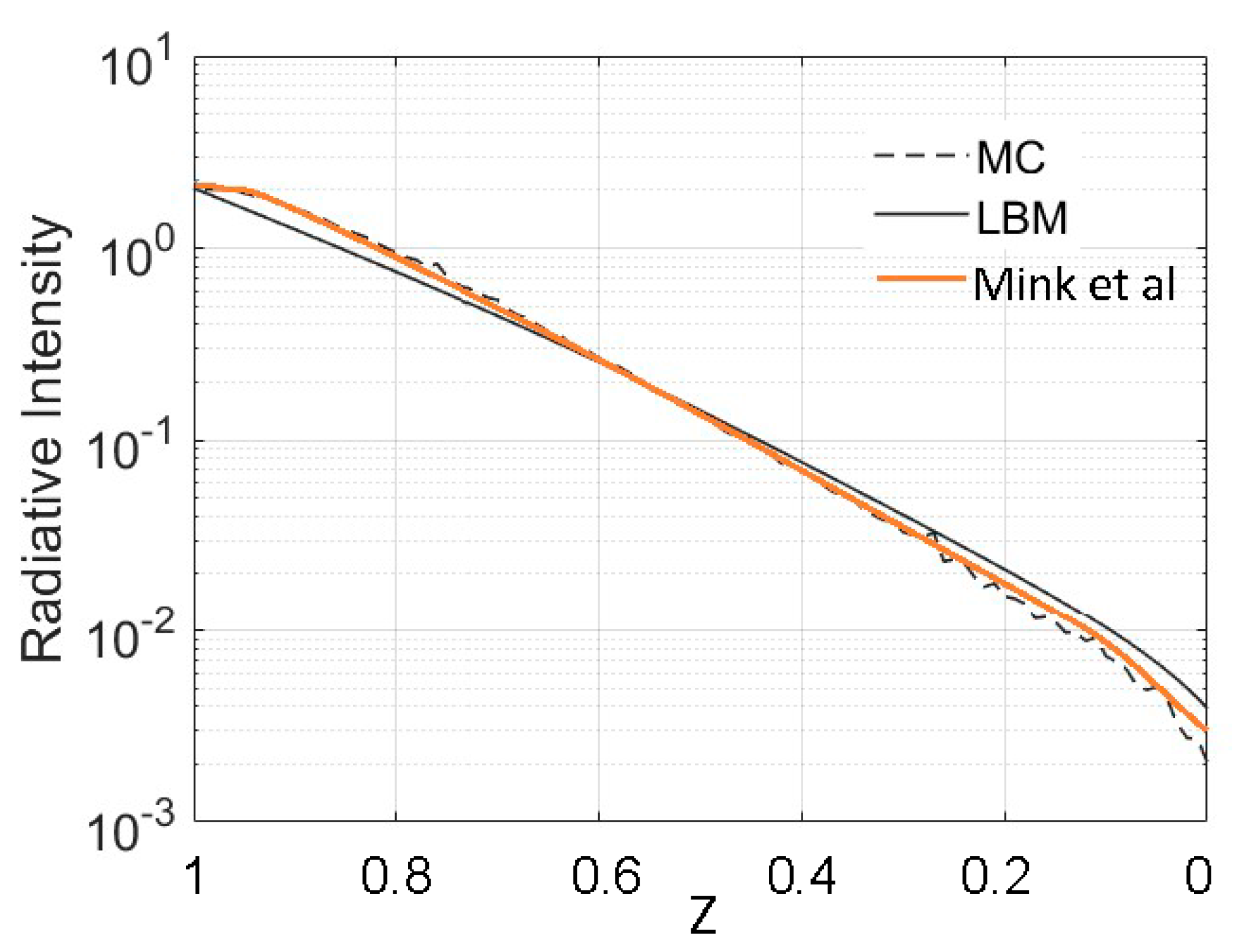
Figure 3 shows the simulation results of the plane (Y = 0.5) with RT-LBM (left panel) and the MC model (right panel). In these simulations, the entire top boundary was a prescribed radiation beam with a unit of intensity and the other boundaries were black walls. The simulation parameters were a = 0.9 and b = 12, which is optically very thick as in a clouded atmosphere or atmospheric boundary layer in a forest fire situation [31]. The two simulation methods produced similar radiation fields in most areas except the MCM produced slightly greater radiative intensity near the top boundary. Near the side boundaries, the radiative intensity values were smaller due to less scattering of the beam radiation near the black boundaries. This case is also simulated in Mink et al. [29] with their MC model. Figure 4 is a plot of the radiative intensities along the line at the center of the computation domain using these three models. The simulation results from the three methods compare well. First, the results from the two MC models agree well, which validates the correctness of our own MC model. There are small differences near the top boundary between RT-LBM and the MC models. The reason for over-estimation near the incoming boundary area is caused by a small effect of false anisotropic radiative transport in LBM where only the direct beam radiation is specified in the incoming boundary. However, after penetration of two times of the free path lengths, the diffuse radiation becomes dominant and the results are much closer to the MC. Since the optical depth is very high, the radiation intensity from the top boundary to the bottom boundary gradually has a two orders of magnitude reduction. The MC model produced a radiative intensity field that had very little fluctuation in the contour plots (Figure 2), indicating that the 109 photons release in this simulation is adequate for removing the statistical noise.
3.2. Direct Solar Radiation from a Top Boundary Window
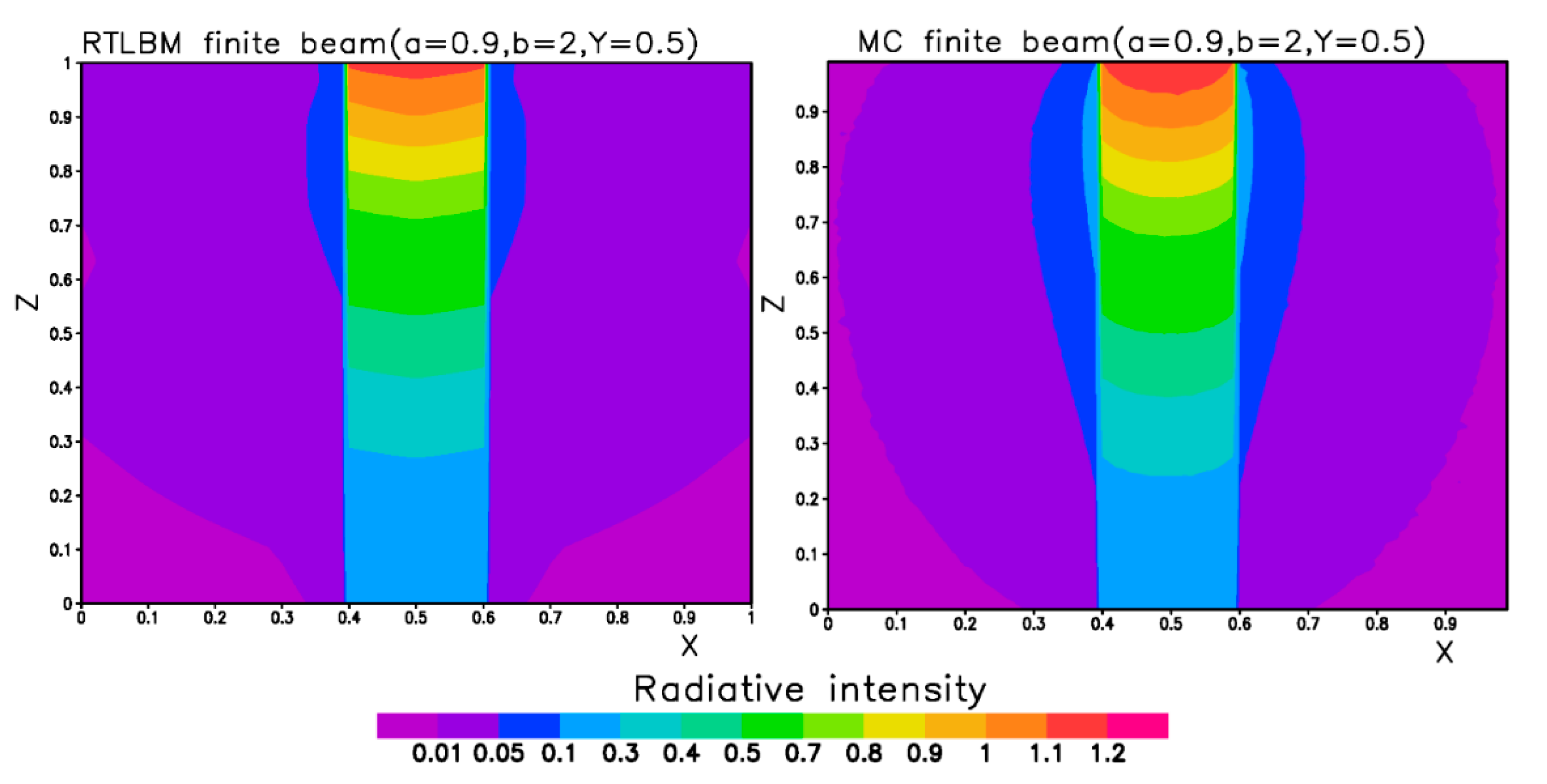
In this case, a perpendicular incoming beam entered a window (0.2 × 0.2) in the middle of the top boundary (Figure 2b). The parameters (a = 0.9, b = 2) of the particular medium are comparable to episodes of heavily polluted atmosphere in some urban areas [33,34,35]. The LBM simulation was also evaluated with our MC model and other MC model [29] results.
Figure 5 compares our RT-LBM and the MC simulations. The results between the two models matched reasonably well except at the area at the top of the window. Again, the MC model produced slightly larger radiative intensity values near the radiation entrance window. The other area, away from perpendicular to the incoming window, also had much smaller values due to the scattering of the direct beam area for this relatively medium optical depth and large scattering albedo. Some difference between RT-LBM and the MC model was observed in these low-intensity areas. The RT-LBM-simulated slightly smaller values near the incoming radiation boundary are also reported in Mink et al. [29]. Figure 6 compares the line samples in the z direction (Y = 0.5; X = 0.5, 0.75, 0.85) for RT-LBM, our MC model, and the other MC model [29] simulations. The simulations compare well in the centerline, excepting slight differences near the window area. The radiation intensity compares reasonably well but there are slightly more differences off the centerline.
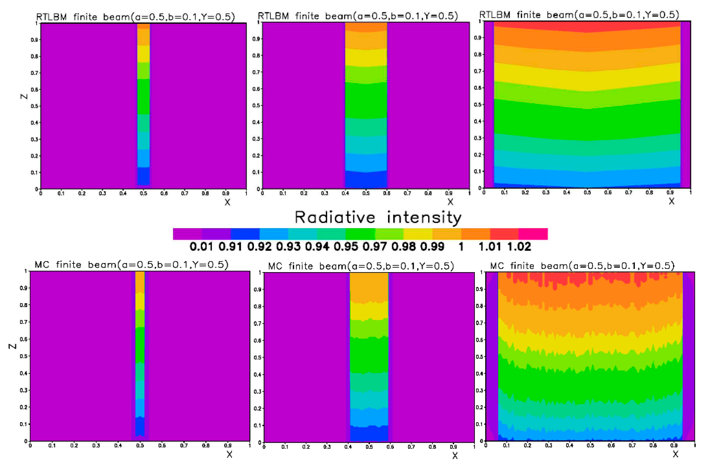
To analyze the effect of window size on radiative intensity, we conducted multiple runs with different window sizes (0.05 × 0.05, 0.2 × 0.2, and 0.9 × 0.9) but with identical radiation intensities prescribed at the incoming window. Figure 7 displays the X-Z cross section at Y = 0.5. The medium parameters, a = 0.5 and b = 0.1, resemble a typical clean atmosphere [36]. In spite of more fluctuations, in the MC simulation results many more photon particles (1012) were released (Figure 7, bottom panel) due to the low optical depth in clean air, and the RT-LBM and MC simulations compare reasonably well. The variation of the centerline radiative intensity values was less than 5% with the larger window size having a slight greater radiative intensity. In these cases of the lower scattering albedo (Figure 7 and Figure 8), the differences between RT-LBM and the MC model are much smaller near the incoming boundary compared with the case of large scattering albedo (Figure 4). This analysis indicates that very clean atmospheric conditions can be parameterized without much error using a single computation given an identical boundary or very similar boundary conditions.
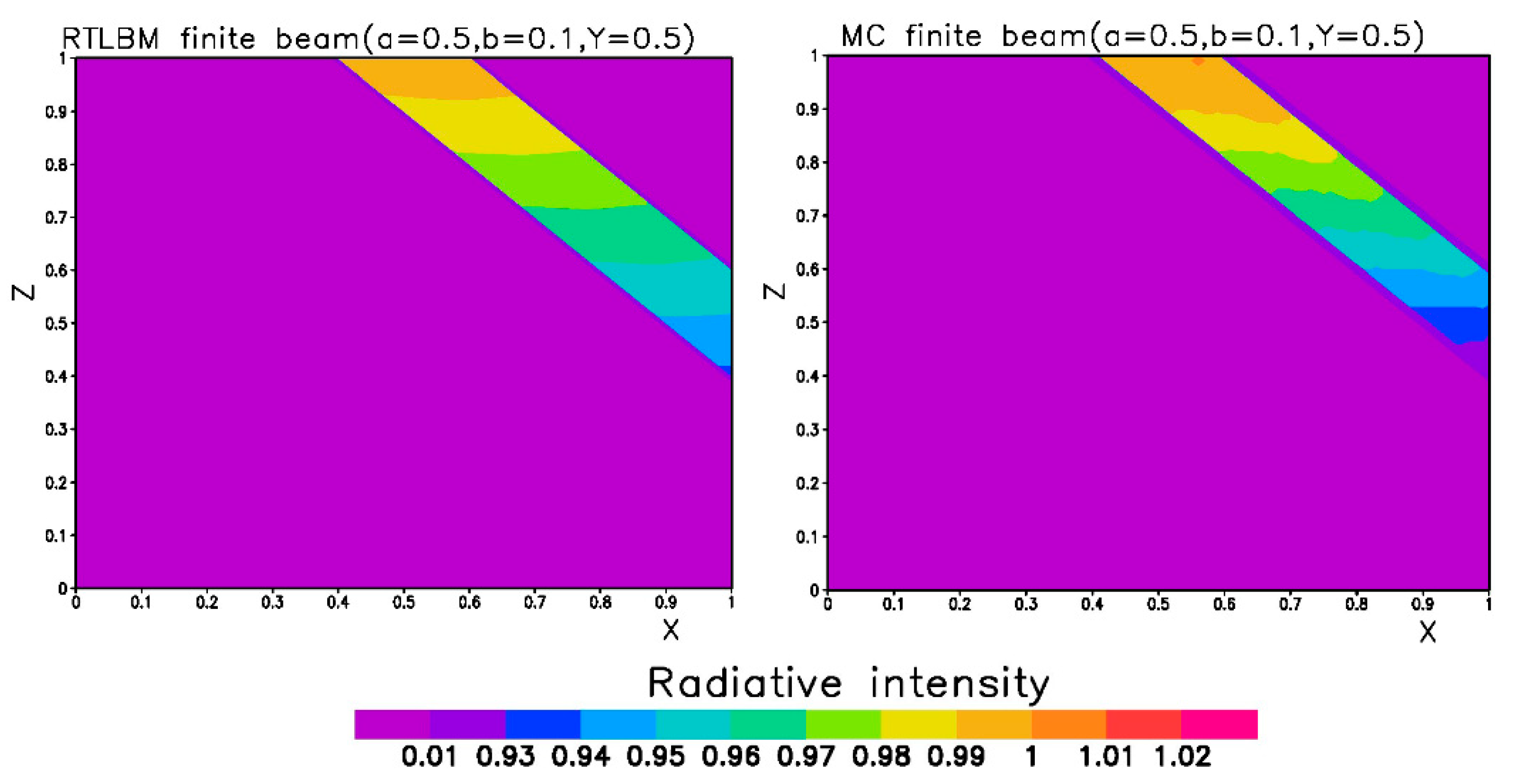
Another situation, of solar direct beam radiation oblique to the level ground surface, is simulated. The atmospheric optical parameters of a clean air (a = 0.5, b = 0.1) situation were used. The motivation for this simulation was to look into whether direct solar radiation decreases when the solar ray is not perpendicular to the top boundary surface. The incoming solar zenith angle was set to 45° from the west and the incoming direct solar radiative intensity was set to one. The RT-LBM and MC simulations compare reasonably well (Figure 8). The decaying of the solar radiative intensity along the centerline of the perpendicular to window (Figure 7) and oblique to the window at 45° shows small differences between the perpendicular and oblique cases. This comparison analysis indicates that a perpendicular-to-window simulation can be used to approximate the radiative intensity for different solar elevation angles, which has a very significant implication for reducing the radiation computation in a situation where the atmospheric optical parameters are constant and vertically homogenous.
3.3. GPU Implementation of RT-LBM and Computational Speed
In solving the complex RTE, RT-LBM uses the typical collision and streaming steps that the LBM used to solve fluid simulations [30,31]. By writing the Equation (4) in the following form,
The complex scattering and absorption processes in the RTE are computed within each node (Figure 1) by a photon-medium collision process (Equation (16)), while a streaming process of photons is handled by simple linear propagation between the neighbor grid nodes (Equation (17)). This makes the LBM very effective within the massive parallelization of the GPU architecture. Modern GPUs have thousands of compute cores and thus are capable of running thousands of threads simultaneously. In the LBM algorithm, the data locality is satisfied and time-stepping is explicit. Each computation grid cell in the domain is assigned to a GPU thread. The entire computation procedure described in Section 2.1 can be summarized in following pseudo-code:
- Set up the radiation parameters and computation grids;
- For each iteration time step t do;
- For each lattice node x do;
- If node x is a boundary point then;
- Apply the boundary conditions;
- End if;
- Compute the equilibrium pdf (Equation (9));
- Compute collision term (Equation (16));
- Update (propagate) the pdf for next time step (Equation (17));
- Compute the radiation intensity (Equation (5));
- End do;
- Check the convergence (Equation (18));
- End do.
The model code is written in NVidia CUDA (Common Unified Device Architecture). In our implementation, the 3-D computation grids are mapped to 1-D memory. In GPUs, threads execute in lockstep in group sets called warps. The threads within each warp need to load memory together in order to use the hardware most effectively. This is called memory coalescing. In our implementation, we manage this by ensuring threads within a warp are accessing consecutive global memory as often as possible. For instance, when calculating the PDF vectors in Equation (15), we must load all 26 lattice PDFs per grid cell. We organize the PDFs such that all the values for each specific direction are consecutive in memory. In this way, as the threads of a warp access the same direction across consecutive grid cells, these memory accesses can be coalesced.
A common bottleneck in GPU-dependent applications is transferring data between main memory and GPU memory. In our implementation, we are performing the entire simulation on the GPU and the only time data need to be transferred back to the CPU during the simulation is when we calculate the error norm to check the convergence. In our initial implementation, this step was conducted by first transferring the radiation intensity data for every grid cell to main memory each time step and then calculating the error norm on the CPU. To improve performance, we only check the error norm every 10 time steps. This leads to a 3.5× speedup over checking the error norm every time step for the 1013 domain case.
This scheme is sufficient, but we took it a step further, implementing the error norm calculation itself on the GPU. To achieve this, we implement a parallel reduction to produce a small number of partial sums of the radiation intensity data. It is this array of partial sums that is transferred to main memory instead of the entire volume of radiation intensity data. On the CPU, we calculate the final sums and complete the error norm calculation. This new implementation only results in a 1.32× speedup (1013 domain) over the previous scheme of checking only every 10 time steps. However, we no longer need to check the error norm at a reduced frequency to achieve similar performance; checking every 10 time steps is only 0.057× faster (1013 domain) than checking once a frame using GPU-accelerated calculation. In the tables below, we opted to use the GPU calculation at 10 frames per second but it is comparable to the results of checking every frame.
Table 1 and Table 2 list the computational efficiency of our RT-LBM. A computational domain with a direct top beam (Figure 2 and Figure 3) was used for the demonstration. In order to see the domain size effect on computation speed, the computation was carried out for different numbers of the computational nodes (101 × 101 × 101 and 501 × 501 × 201). The RTE is a steady-state equation, and many iterations are required to achieve a steady-state solution. These computations are considered to converge to a steady-state solution when the error norm is less than 10−6. The normalized error or error norm at iteration time step t is defined as:
where I is the radiation intensity at grid nodes, is the grid node index, and N is the total number of grid points in the entire computation domain.
The single-thread CPU computation using a FORTRAN version of the code, which is slightly faster than the code in C, is used for the computation speed comparison. The speed of the RT-LBM model and MC model in a same CPU are compared for the first case only to demonstrate that the MC model is much slower than the RT-LBM. RT-LBM in the CPU is about 10.36 times faster than the MC model from the first domain setup using the CPU. A NVidia Tesla V100 (5120 cores, 32 GB memory) was run to observe the speed-up factors for the GPU over the CPU. The CPU used for the RT-LBM model computation is an Intel CPU (Intel Xeon CPU at 2.3 GHz). For the domain size of 101 × 101 × 101, the Tesla V100 GPU showed a 39.24 times speed-up compared with single CPU processing (Table 1). It is worthwhile noting the speed-up factor of RT-LBM (GPU) over the MC model (CPU) was 406.53 (370/0.91) times if RT-LBM was run on a Tesla V100 GPU. For the much larger domain size, 501 × 501 × 201 grid nodes (Table 2), the RT-LBM in the Tesla V100 GPU had a 120.03 times speed-up compared with the Intel Xeon CPU at 2.3 GHz. These results indicated the GPU is even more effective in speeding up RT-LBM computations when the computational domain is much larger, which is consistent with what we found with the LBM fluid flow modeling [30]. We are in the process of extending our RT-LBM implementation to multiple GPUs which will be necessary in order to handle even larger computational domains.
The computational speed-up of RT-LBM using the single GPU over CPU is not as great as in the case of turbulent flow modeling [30], which showed a 200 to 500 speed-up using older NVidia GPU cards. The reason is turbulent flow modeling uses a time-marching transient model, while RT-LBM is a steady-state model, which requires many more iterations to achieve a steady-state solution. Nevertheless, the GPU speed-up of 120 times in RT-LBM is significant for implementing radiative transfer modeling which is computationally expensive.
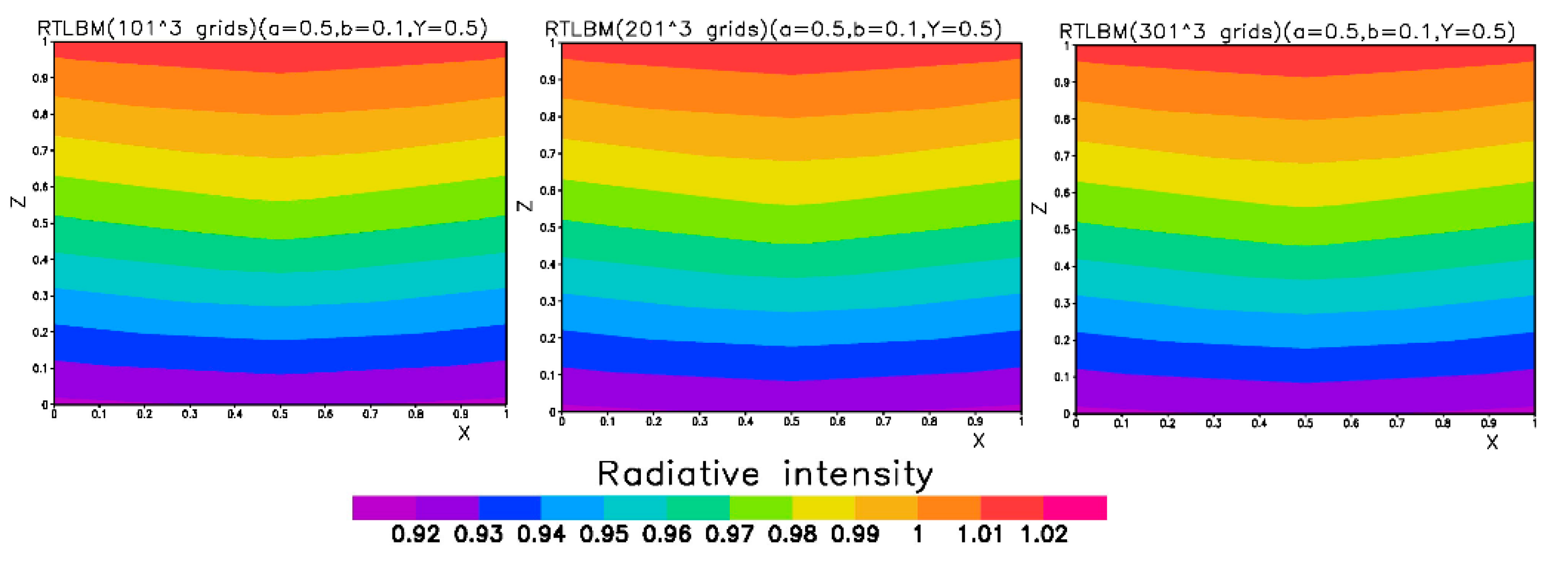
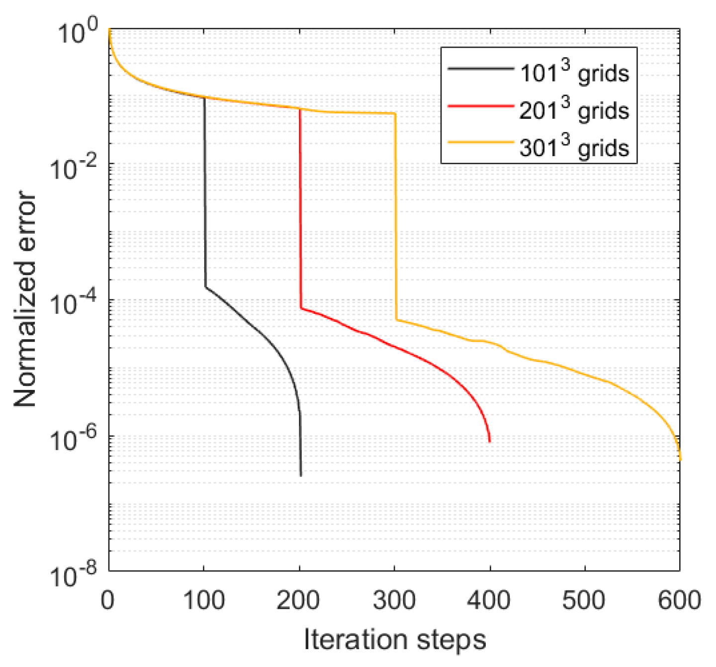
The model code is also tested for the grid dependency by computing the radiation field in a same domain using three different grid densities. Figure 9 shows the radiation intensities in three different grid densities (1013, 2013, and 3013 computation grids). The convergence criteria were set to be 10−5 for the error norm. The LBM model produced very similar radiation fields that are hard to see the differences visually. This fact indicates that 10−5 error norm for convergence criteria is probably good enough for this model domain situation. The convergence behaviors of the different densities of computation grids were also recorded at each iteration step and plotted in Figure 10. The three different grid densities showed a similar trend in convergence behavior with respect to iteration time. The iteration time to reach a same small error norm of 10−6 for denser grids requires many more steps of iterations. In these simulations, the Courant number are all equal to one. Numerical stable algorithm was assured and also observed.
The unit conversion in LBM fluid modeling is complex [37]. However, in this steady-state radiative transfer modeling, the time step is only for the iteration computation and there is no problem to map the non-dimensional variables to variables’ units. Since the LBM-RT in this paper is a steady-state problem, only conversions are needed between physical length and non-dimensional length, and the scattering and absorption coefficients and non-dimensional parameters a and b (a scattering albedo, b optical depth) can be transformed using Equations (10) and (11). The radiation intensity can be converted to a physical unit by multiplying the value of incoming boundary intensity with a physical unit.
4. Discussion and Conclusions
This paper reported a newly developed radiative transfer model using the lattice Boltzmann method, RT-LBM, for applications in atmospheric environments. The test results indicated the new RT-LBM has reasonably accurate results compared with traditional MC models. The model takes advantage of the LBM algorithms of collision and streaming to accelerate the computation speed. The implementation of RT-LBM using the GPU has realized a computation speed-up of 120 times faster than a CPU implementation for a very large domain. RT-LBM also had a 10 times speed-up over the MC model for a same radiative case on the same CPU, which makes a total of a 406 times speed-up for RT-LBM on a GPU over the MC model on a CPU.
The atmospheric environment is a complex composite of many different gases, aerosols, and hydrometers, and the composition is very dynamic. The optical parameters are often very different for different wavelengths of radiation. In atmospheric radiative transfer modeling, many runs for different spectral lengths with different optical parameters must be made to complete the entire radiative energy transfer domain. Since radiative modeling is computationally intensive, the newly developed RT-LBM provides advantages. However, many research areas, such as complex boundary specification, anisotropic scattering by large aerosols, and optical parameters specification, need to be carried out to realize the potential of this new method for specific applications. Some applications, such as for solar energy, are feasible with RT-LBM using broadband optical parameters to reduce the complexity. In this case, solar radiation can be divided into two spectral bands, shortwave and longwave. Two different sets of bulk optical parameters can be used for solar shortwave radiation and longwave radiation from the ground surface.
Author Contributions
Conceptualization, RT-LBM, Y.W.; methodology, Y.W.; software, J.D., Y.W. and X.Z.; formal analysis, Y.W.; MC modeling, X.Z. All authors have read and agreed to the published version of the manuscript.
Funding
This research received no external funding.
Institutional Review Board Statement
This paper was reviewed and approved by authors’ institution.
Informed Consent Statement
Not applicable.
Data Availability Statement
Data is contained within the article.
Conflicts of Interest
The authors declare no conflict of interest.
References
- Howell, J.R. The Monte Carlo method in radiative heat transfer. J. Heat Transfer. 1998, 120, 547–560. [Google Scholar] [CrossRef]
- Chai, J.C.; Lee, H.S.; Patankar, S.V. Finite volume method for radiation heat transfer. J. Thermophys. Heat Transfer. 1994, 8, 419–425. [Google Scholar] [CrossRef]
- Coelho, J.P. Advances in the discrete ordinates and finite volume methods for the solution of radiative heat transfer problems in participating media. J. Quant. Spectrosc. Radiat. Transf. 2014, 145, 121–146. [Google Scholar] [CrossRef]
- Hunter, B.; Guo, Z. Comparison of quadrature schemes in DOM for anisotropic scattering radiative transfer. Numer. Heat Transf. Part B 2013, 63, 485–507. [Google Scholar] [CrossRef]
- Qian, Y.-H.; d’Humières, D.; Lallemand, P. Lattice BGK models for Navier-Stokes equation. Europhys. Lett. 1992, 17, 479–484. [Google Scholar] [CrossRef]
- Chen, H.; Chen, S.; Matthaeus, W.H. Recovery of the Navier-Stokes equations using a lattice-gas Boltzmann method. Phys. Rev. A 1992, 45, 5339–5342. [Google Scholar] [CrossRef]
- He, X.; Luo, L.-S. Theory of lattice Boltzmann method: From the Boltzmann equation to the lattice Boltzmann equation. Phys. Rev. E 1997, 56, 6811–6817. [Google Scholar] [CrossRef] [Green Version]
- Chen, S.; Doolen, G.D. Lattice Boltzmann method for fluid flows. Annu. Rev. Fluid Mech. 1998, 30, 329–364. [Google Scholar] [CrossRef] [Green Version]
- d’Humières, D.; Ginzburg, I.; Krafczyk, M.; Lallemand, P.; Luo, L.-S. Multiple-relaxation-time lattice Boltzmann models in three dimension. Phil. Trans. R. Soc. Lond. A 2002, 360, 437–451. [Google Scholar] [CrossRef]
- Aidun, C.K.; Clausen, J.R. Lattice-Boltzmann method for complex flows. Annu. Rev. Fluid Mech. 2010, 42, 439–472. [Google Scholar] [CrossRef]
- Guo, Z.; Shu, C. Lattice Boltzmann Method and Its Applications in Engineering, Advances in Computational Fluid Dynamics; World Scientific Publishing Co.: Singapore, 2013; Volume 3, ISBN 978-981-4508-29-2. [Google Scholar]
- Geist, R.; Rasche, K.; Westall, J.; Schalkoff, R. Lattice-Boltzmann lighting. In Eurographics Workshop on Rendering; Keller, A., Jensen, H.W., Eds.; The Eurographics Association: Norrköping, Sweden, 2004; pp. 355–362. [Google Scholar] [CrossRef]
- Geist, R.; Steele, J. A lighting model for fast rendering of forest ecosystems. In Proceedings of the 2008 IEEE Symposium on Interactive Ray Tracing, Los Angeles, CA, USA, 9–10 August 2008; pp. 99–106. [Google Scholar] [CrossRef] [Green Version]
- Oxenius, J. Kinetic Theory of Particles and Photons: Theoretical Foundations of Non-LTE Plasma Spectroscopy; Springer: Berlin/Heidelberg, Germany, 2012. [Google Scholar] [CrossRef] [Green Version]
- Asinari, P.; Mishra, S.C.; Borchiellini, R. A lattice Boltzmann formulation for the analysis of radiative heat transfer problems in a participating medium. Numer. Heat Transf. Part B 2010, 57, 126–146. [Google Scholar] [CrossRef] [Green Version]
- Mishra, S.C.; Poonia, H.; Das, A.K.; Asinari, P.; Borchiellini, R. Analysis of conduction- radiation heat transfer in a 2D enclosure using the lattice Boltzmann method. Numer. Heat Transf. Part A 2014, 66, 669–688. [Google Scholar] [CrossRef]
- Ma, Y.; Dong, S.; Tan, H. Lattice Boltzmann method for one-dimensional radiation transfer. Phys. Rev. E 2011, 84, 016704. [Google Scholar] [CrossRef] [PubMed]
- Bindra, H.; Patil, D.V. Radiative or neutron transport modeling using a lattice Boltzmann equation framework. Phys. Rev. E 2012, 86, 016706. [Google Scholar] [CrossRef] [PubMed]
- McCulloch, R.; Bindra, R. Coupled radiative and conjugate heat transfer in participating media using lattice Boltzmann methods. Comput. Fluids 2016, 124, 261–269. [Google Scholar] [CrossRef]
- Cifuentes, J.A.B.; Borelli, D.; Cammi, A.; Lomonaco, G.; Misale, M. Lattice Boltzmann Method Applied to Nuclear Reactors—A Systematic Literature Review. Sustainability 2020, 12, 7835. [Google Scholar] [CrossRef]
- Gairola, A.; Bindra, H. Lattice Boltzmann method for solving non-equilibrium radiative transport problems. Ann. Nucl. Energy 2017, 99, 151–156. [Google Scholar] [CrossRef] [Green Version]
- Zhang, Y.; Yi, H.-L.; Tan, H.-P. Lattice Boltzmann method for short-pulsed laser transport in multi-layered Medium. J. Quant. Spectrosc. Radiat. Transf. 2015, 155, 75–89. [Google Scholar] [CrossRef]
- Yi, H.-L.; Yao, F.-J.; Tan, H.-P. Lattice Boltzmann model for a steady radiative transfer equation. Phys. Rev. E 2016, 94, 023312. [Google Scholar] [CrossRef]
- Weih, L.R.; Gabbana, A.; Simeoni, D.; Rezzolla, L.; Succi, S.; Tripiccione, R. Beyond moments: Relativistic lattice Boltzmann methods for radiative transport in computational astrophysics. Mon. Not. R. Astron. Soc. 2020, 498, 3374–3394. [Google Scholar] [CrossRef]
- Liu, X.; Huang, Y.; Wang, C.-H.; Zhu, K. A multi-relaxation-time Boltzmann model for radiative transfer equation. J. Comput. Phys. 2021, 429, 110007. [Google Scholar] [CrossRef]
- McHardy, C.; Horneber, T.; Rauh, C. New lattice Boltzmann method for the simulation of three-dimensional radiation transfer in turbid media. Opt. Express 2016, 24, 16999–17017. [Google Scholar] [CrossRef]
- McHardy, C.; Horneber, T.; Rauh, C. Spectral simulation of light propagation in participating media by using a lattice Boltzmann method for photons. Appl. Math. Comput. 2018, 319, 59–70. [Google Scholar] [CrossRef]
- Mink, A.; Thäter, G.; Nirschl, H.; Krause, M.J. A 3D lattice Boltzmann method for light simulation in participating media. J. Comput. Sci. 2016, 17, 431–437. [Google Scholar] [CrossRef]
- Mink, A.; McHardy, C.; Bressel, L.; Rauh, C.; Krause, M.J. Radiative transfer lattice Boltzmann methods: 3D models and their performance in different regimes of radiative transfer. J. Quant. Spectrosc. Radiat. Transf. 2020, 243, 106810. [Google Scholar] [CrossRef]
- Wang, Y.; Benson, M. Large-eddy simulation of turbulent flows over an urban building array with the ABLE-LBM and comparison with 3D MRI observed data sets. Environ. Fluid Mech. 2020, 21, 287–304. [Google Scholar] [CrossRef]
- Wang, Y.; Decker, J.; Pardyjak, E. Large-eddy simulations of turbulent flows around buildings using a Lattice Boltzmann model. J. App. Meteorol. Climat. 2020, 59, 885–899. [Google Scholar] [CrossRef] [Green Version]
- Chandrasekhar, S. Radiative Transfer; Dover: New York, NY, USA, 1960; p. 393. ISBN 978-0-486-60590-6. [Google Scholar]
- Raffuse, S.M.; McCarthy, M.C.; Craig, K.J.; DeWinter, J.L.; Jumbam, L.K.; Fruin, S.; Gauderman, W.J.; Lurmann, F.W. High-resolution MODIS aerosol retrieval during wildfire events in California for use in exposure assessment. J. Geophys. Res. Atmos. 2013, 118, 11242–11255. [Google Scholar] [CrossRef]
- Li, J.; Liu, R.; Liu, S.C.; Shiu, C.-J.; Wang, J.; Zhang, Y. Trends in aerosol optical depth in northern China retrieved from sunshine duration data, 2016. Geophys. Res. Lett. 2016, 43, 431–439. [Google Scholar] [CrossRef] [Green Version]
- Pandithurai, G.; Dipu, S.; Dani, K.K.; Tiwari, S.; Bisht, D.S.; Devara, P.C.S.; Pinker, R.T. Aerosol radiative forcing during dust events over New Delhi, India. J. Geophys. Res. 2008, 113, D13209. [Google Scholar] [CrossRef]
- Mulcahy, J.P.; O’Dowd, C.D.; Jennings, S.G. Aerosol optical depth in clean marine and continental northeast Atlantic air. J. Geophys. Res. 2009, 114, D20204. [Google Scholar] [CrossRef] [Green Version]
- Baakeem, S.; Saleh, A.; Bawazeer, S.A.; Mohamad, A.A. A novel approach of unit conversion in the lattice Boltzmann method. App. Sci. 2021, 11, 6386. [Google Scholar] [CrossRef]
Figure 1.
D3Q26 lattice used in RT-LBM. The numbered arrows are the lattice directions of the photon propagation to neighbor lattice nodes.
Figure 1.
D3Q26 lattice used in RT-LBM. The numbered arrows are the lattice directions of the photon propagation to neighbor lattice nodes.

Figure 2.
Three types of incoming radiation boundaries (a–c) and setups for the simulations. The red vertical planes are the Z-X cross sections at Y = 0.5, which are plotted in the Results section.
Figure 2.
Three types of incoming radiation boundaries (a–c) and setups for the simulations. The red vertical planes are the Z-X cross sections at Y = 0.5, which are plotted in the Results section.

Figure 3.
Comparison of the simulation results from RT-LBM (left panel) and the MC model (right panel). The X-Z cross sections (Y = 0.5) are from the 3-D radiative intensity fields. The radiative parameters are a = 0.9 and b = 12.
Figure 3.
Comparison of the simulation results from RT-LBM (left panel) and the MC model (right panel). The X-Z cross sections (Y = 0.5) are from the 3-D radiative intensity fields. The radiative parameters are a = 0.9 and b = 12.

Figure 4.
Comparison of the radiative intensity along the Z lines (X = 0.5, Y = 0.5) for RT-LBM, the MC model, and the MC model from Mink et al. (2020). The radiative parameters are a = 0.9 and b = 12.
Figure 4.
Comparison of the radiative intensity along the Z lines (X = 0.5, Y = 0.5) for RT-LBM, the MC model, and the MC model from Mink et al. (2020). The radiative parameters are a = 0.9 and b = 12.

Figure 5.
Windowed simulation results from RT-LBM (left panel) and the MC model (right panel). The X-Z cross sections (Y = 0.5) are from the 3-D radiative intensity fields. The radiative parameters are a = 0.9, b = 2.
Figure 5.
Windowed simulation results from RT-LBM (left panel) and the MC model (right panel). The X-Z cross sections (Y = 0.5) are from the 3-D radiative intensity fields. The radiative parameters are a = 0.9, b = 2.

Figure 6.
Windowed simulation comparison of the radiative intensity along the Z lines (X = 0.5, Y = 0.5, 0.75, 0.88) for RT-LBM, our MC model, and the MC model (MCM) from Mink et al. (2020). The radiative parameters are a = 0.9, b = 2.
Figure 6.
Windowed simulation comparison of the radiative intensity along the Z lines (X = 0.5, Y = 0.5, 0.75, 0.88) for RT-LBM, our MC model, and the MC model (MCM) from Mink et al. (2020). The radiative parameters are a = 0.9, b = 2.

Figure 7.
Different window size effects on the direct solar radiation intensity. The top row are from RT-LBM simulations. The bottom row are from MC model simulations. The radiative parameters are a = 0.5, b = 0.1.
Figure 7.
Different window size effects on the direct solar radiation intensity. The top row are from RT-LBM simulations. The bottom row are from MC model simulations. The radiative parameters are a = 0.5, b = 0.1.

Figure 8.
Oblique incoming solar direct beam radiation simulation case. Comparison of the radiative intensity at X-Z cross section at Y = 0.5. for RT-LBM and the MC model. The radiative parameters are a = 0.5, b = 0.1.
Figure 8.
Oblique incoming solar direct beam radiation simulation case. Comparison of the radiative intensity at X-Z cross section at Y = 0.5. for RT-LBM and the MC model. The radiative parameters are a = 0.5, b = 0.1.

Figure 9.
The plots of vertical (Y = 0.5) cross-sections of radiation intensities with different computation grid densities (left: 1013, center: 2013, and right: 3013). The radiation parameters (a = 0.5, b = 0.1) and the domain sizes are the same for these three runs.
Figure 9.
The plots of vertical (Y = 0.5) cross-sections of radiation intensities with different computation grid densities (left: 1013, center: 2013, and right: 3013). The radiation parameters (a = 0.5, b = 0.1) and the domain sizes are the same for these three runs.

Figure 10.
The convergence behaviors of the model simulations with three different grid densities.


Table 1.
Computation time for a domain with 101 × 101 × 101 grid nodes.
| CPU Xeon 3.1 GHz (Seconds) | Tesla GPU V100 (Seconds) | GPU Speed Up Factor (CPU/GPU) | |
|---|---|---|---|
| RT-MC | 370 | 406.53 | |
| RT-LBM | 35.71 | 0.91 | 39.24 |
Table 2.
Computation time for a domain with 501 × 501 × 201 grid nodes.
| CPU Xeon 3.1 GHz (Seconds) | Tesla GPU V100 (Seconds) | GPU Speed Up Factor (CPU/GPU) | |
|---|---|---|---|
| RT-LBM | 3632.14 | 30.26 | 120.03 |
Publisher’s Note: MDPI stays neutral with regard to jurisdictional claims in published maps and institutional affiliations. |
© 2021 by the authors. Licensee MDPI, Basel, Switzerland. This article is an open access article distributed under the terms and conditions of the Creative Commons Attribution (CC BY) license (https://creativecommons.org/licenses/by/4.0/).
Share and Cite
MDPI and ACS Style
Wang, Y.; Zeng, X.; Decker, J. A GPU-Accelerated Radiation Transfer Model Using the Lattice Boltzmann Method. Atmosphere 2021, 12, 1316. https://0-doi-org.brum.beds.ac.uk/10.3390/atmos12101316
AMA Style
Wang Y, Zeng X, Decker J. A GPU-Accelerated Radiation Transfer Model Using the Lattice Boltzmann Method. Atmosphere. 2021; 12(10):1316. https://0-doi-org.brum.beds.ac.uk/10.3390/atmos12101316
Chicago/Turabian StyleWang, Yansen, Xiping Zeng, and Jonathan Decker. 2021. "A GPU-Accelerated Radiation Transfer Model Using the Lattice Boltzmann Method" Atmosphere 12, no. 10: 1316. https://0-doi-org.brum.beds.ac.uk/10.3390/atmos12101316
Note that from the first issue of 2016, this journal uses article numbers instead of page numbers. See further details here.