
Spectral Recalibration of NOAA HIRS Longwave CO2 Channels toward a 40+ Year Time Series for Climate Studies


1
Earth System Science Interdisciplinary Center, Cooperative Institute for Satellite Earth System Studies (CISESS), University of Maryland, College Park, MD 20740, USA
2
Center for Satellite Applications and Research, NOAA National Environmental Satellite, Data, and Information Service, College Park, MD 20740, USA
*
Author to whom correspondence should be addressed.
Atmosphere 2021, 12(10), 1317; https://0-doi-org.brum.beds.ac.uk/10.3390/atmos12101317
Submission received: 1 September 2021
/
Revised: 1 October 2021
/
Accepted: 4 October 2021
/
Published: 9 October 2021
(This article belongs to the Special Issue Advanced Technologies in Satellite Observations)
Abstract
:The High-Resolution Infrared Radiation Sounder (HIRS) on NOAA and MetOp A/B satellites has been observing the Earth continuously for over four decades, providing essential data for operational numerical weather prediction, retrieval of atmospheric vertical profile, and total column information on atmospheric temperature, moisture, water vapor, ozone, cloud climatology, and other geophysical parameters globally. Although the HIRS data meets the needs of the short-term weather forecast, there are inconsistencies when the long-term decadal time series is used for time series analysis. The discrepancies are caused by several factors, including spectral response differences between the HIRS models on the satellites and spectral response uncertainties and other calibration issues. Previous studies have demonstrated that significant improvements can be achieved by recalibrating some of the HIRS longwave CO2 channels (Channels 4, 5, 6, and 7), which has helped make the time series more consistent. The current study aims to extend the previous study to the remaining longwave infrared sounding channels, including Channels 1, 2, 3, and 8, using a similar approach. Similar to previous findings, the spectral shift of the HIRS bands has helped improve the consistency in the time series from NOAA-06 to MetOp-A and B for these channels. We also found that HIRS channels on MetOp-B also have bias relative to Infrared Atmospheric Sounding Interferometer (IASI) on the same satellite, especially Channel 4, and a spectral shift significantly reduced the bias. To bridge the observation gap in time series in the mid-1980s between NOAA-07 and NOAA-09, the global mean method has been used since no transfer radiometers between them was available for this period, and the spectral response function corrections, therefore, can be applied to the earliest satellites (NOAA-06) for these channels. The recalibration parameters have been provided to other scientists at the University of Wisconsin for improving the time series in their long-term studies using historical HIRS data and are now made available to the science community.
1. Introduction
The NOAA TIROS-N series of satellites from NOAA-06 in the late 1970s to current NOAA-19 and MetOp A and B by EUMETSAT, with infrared channels sensing atmospheric vertical layers, have provided valuable datasets serving the weather forecasting and climate analysis. High-Resolution Infrared Radiation Sounder (HIRS) is one of the main instruments onboard these satellites with 12 long-wave infrared channels (6.5 um to 15 um), seven short wave infrared channels (3.7 um to 4.6 um), and one visible channel (0.69 um). Of the 12 infrared channels, Channels 1–7 are the CO2 channels, Channel 8 is a window channel, Channel 9 for ozone, Channel 10 as a split-window channel, and Channels 11 and 12 are water vapor channels. Due to its long time series, high observation frequency, and relatively high resolution with global coverage, the HIRS measurements have been used to monitor the Earth’s climate change. Many climate data records based on the HIRS measurements have been developed, such as the cloud climatology [1,2,3], upper tropospheric water vapor time series [4,5], outgoing longwave radiation (OLR) [6] and ENSO index [7].
The HIRS instrument design has evolved over the four decades, from HIRS/2, HIRS/2I, HIRS/3 on the earlier satellites to HIRS/4 onboard NOAA-18, NOAA-19, and MetOp-A/B [6]. The onboard blackbody calibrators used for calibration changed from two on HIRS/2 and HIRS/2I to one on HIRS/3 and HIRS/4. The HIRS/4 has a smaller field of view (FOV) of 10 km compared to about 20 km for earlier HIRS. In addition, for each channel, the spectral response functions (SRF) are different from satellite to satellite due to manufacturing variabilities. The discrepancy in measurements from different instruments onboard different satellites poses a challenge for time series analysis. These discrepancies are mainly caused by the different instrument characteristics, such as the different SRF of the same channel on different satellites and uncertainties in them [8,9,10,11]. The HIRS spectral uncertainties and prelaunch measurement errors in SRF are regarded as major sources of HIRS measurement uncertainties ([12,13]. Cao et al. [9] analyzed the three possible contributions of the SRF differences: (1) relatively loose performance specification and tolerance for the channel spectral center frequency in the instrument design specification, and the filter mounting incident angle deviations, (2) pre-launch SRF measurement uncertainties due to lack of traceability requirement, and (3) pre-launch to after-launch SRF shifts. Cao et al. [10] has compared the HIRS observations with IASI and demonstrated that the SRF uncertainty is the main calibration error for HIRS longwave channels. The longwave CO2 channels (4, 5, and 7), which measure a spectral region with a steep radiometric gradient in the atmospheric spectral absorption curve, are very sensitive to SRF errors. Hence, the bias can be reduced by shifting SRF in the wavenumber space [8]. Due to the design differences mentioned above, the SRF of the same channels on different HIRS instruments has different central wave numbers and shapes. This SRF difference directly affects the inter-satellite bias and becomes an obstacle in constructing climate data records. These inter-satellite biases could be directly subtracted from globally averaged time series during the overlapping periods for some studies [5], or a better approach is to quantify the inter-satellite SRF differences of the same channel and then applied the corrected SRFs [1].
Chen et al. [8] analyzed the CO2 channels for cloud detection (Channels 4, 5, and 7) and found that the inter-satellite bias is significant and can exceed 4% of radiance for the longwave CO2 channels. Therefore, a methodology was developed to reduce the biases through spectral shift using IASI spectra as references, which reduces the uncertainties in the HIRS spectral response functions. The radiometric biases due to HIRS spectral uncertainties can then be estimated based on the correlation between the modeled radiance changes by SRF shift for a given channel and the radiometric values of other relevant channels since these channel radiances for a given atmospheric profile are related to their vertical weighting functions which peak at known atmosphere layers. The modeled relationships between channels are then used to derive the optimal SRF shift from the HIRS inter-satellite bias for one channel and the observed HIRS values for other channels over simultaneous nadir overpasses (SNO) observations. This inter-satellite SRF shift is then propagated from MetOp-A HIRS to the earliest satellites using the long-term SNO time series. Thus, the SRFs of each channel on different satellites can be optimized using IASI/MetOp-A as a reference. In their study, for longwave channels (4, 5, 6, 7), the optimal SRF shift has been derived for NOAA-09 to MetOp-A. Thus, the cloud top pressure climate data record from the longwave CO2 channels can be reconstructed with the accuracy requirement of 1% by The World Meteorological Organization’s Global Climate Observing System (WMO/GCOS) [1].
However, in Chen et al.’s [8] study, there are two tasks that required further explorations. First, they only focused on the four long-wave CO2 channels and left other channels unstudied. Second, there is a SNO gap between NOAA-09 and early satellites due to the lack of overlapping SNOs, so that the optimal SRF shift of NOAA-06, NOAA-07, and NOAA-08 relative to IASI cannot be obtained. As a result, the task of analyzing the remaining longwave channels in this study becomes straightforward. Therefore, in this study, we focus on the remaining longwave temperature sounding channels (Channels 1–3 and 8) to recalibrate their SRFs for early satellite NOAA-06 to the latest MetOp-B.
The same methods by Chen et al. [8] can be used to derive optimal SRF shift for later satellites from NOAA-06 for those unstudied channels. However, the sensitivity of radiance change to SRF shift for the channels in this study is less significant compare to the three longwave CO2 channels in previous studies [8,11], which means more care needs to be taken in dealing with the dataset selection with more strict quality control and criteria than before. Furthermore, the data gap between NOAA-09 and earlier satellites makes the study difficult due to the lack of SNOs between NOAA-09 and any previous satellites (N06–N08) and the lack of similar channels onboard other satellites the same period. Thus, a new method is needed to fill in the gap between these satellites. In addition, Chen et al. [8] studied the inter-satellite correction before MetOp-B (up to 2012). However, after their study, the MetOp-B was launched in 2011 with HIRS/4 onboard. Thus, the calibration also needs to be extended to this latest satellite MetOp-B for the long-term time series.
Chen and Cao [11] introduced the nonlinear calibration and successfully reduced the radiance bias and standard deviation of Channel 8 onboard the MetOp-A, by comparing the recalibrated HIRS radiance and the simulated radiance using hyperspectral radiance of the IASI onboard the same satellite. However, the nonlinearity correction is small (on the order of 0.1 K). This study found that the inter-satellite bias for this channel can be larger, which cannot be explained entirely by the nonlinearity correction. In this study, we will focus on SRF uncertainty while also considering the nonlinearity effects. Chen et al. [8] and Cao et al. [10] have an in-depth discussion on the SRF problems. Similar to Chen et al. [8], we believe that the optimized SRF can be derived by analyzing HIRS and IASI observations using SNO time series.
This paper describes the data and methodology in the next section, followed by the results and analysis in Section 3. Finally, the conclusion and future work are given in the last section.
2. Data and Methodology
2.1. Data Sources
All HIRS Level1B data used in this study are obtained from NOAA/NESDIS/STAR SCDR-files online database. The IASI Level 1C dataset is from NOAA Comprehensive Large Array-data Stewardship System. The IASI data are read out using the Basic ENVISAT Atmospheric Tool Box (BEAT) software Common Data Access Toolbox (CODA) component (https://atmospherictoolbox.org/coda/, accessed on 10 July 2021) in MATLAB and verified using IASI readers in IDL as used in previous studies. The previously found SNO locations/times used by Chen et al. [8] for the analysis of other HIRS channels have been reused here to construct the SNO time series.
2.2. MetOp A/B HIRS SRF Correction Using IASI Spectra
It has previously been demonstrated that IASI hyperspectral radiances are very accurate and in good agreement with other hyperspectral sounder measurements such as AIRS and CrIS. Therefore, IASI can be used as an on-orbit reference standard for calibrating other instruments such as HIRS. In comparison, HIRS is a broadband instrument with 19 spectral channels in the infrared and is not spectrally resolved. MetOp satellites have both IASI and HIRS onboard the same platform. This provides excellent opportunities using IASI to calibrate HIRS on-orbit to resolve the two known issues in HIRS: the SRF differences between satellites (SRFdf) and SRF errors (SRFerr) or uncertainties for each satellite. Therefore, the strategy is relatively straight forward for HIRS on MetOp A and B: the IASI spectra convolution with HIRS spectral response functions, which produces “IASI simulated HIRS radiances” for each HIRS channel. Then, the IASI simulated HIRS radiances are collocated and compared with simultaneous observations from HIRS observed radiances on the same MetOp satellite. If these two do not agree (i.e., a bias exists), then it is believed that HIRS SRFerr or uncertainties cause the bias. By shifting the HIRS SRF and re-convolve with IASI spectra iteratively, an optimized IASI simulated HIRS data will reduce the bias to a minimum, and the corrected HIRS SRF (SRFcor) is therefore obtained.
In comparing IASI simulated HIRS with collocated simultaneous HIRS observations, the standard deviation of the difference between the former and latter in the time series is used as an indicator for optimized SRF correction. The collocation between HIRS and IASI on MetOp-A is relatively easier than that between two satellites since they are on the same satellite. Therefore, only near nadir pixels (for HIRS pixels 26–31) within 3 s and 5 km are used to determine the collocation pairs between HIRS and IASI. The IASI spectra are then convolved with MetOp HIRS SRF to get the IASI simulated HIRS radiance using Equation (1).
where is the IASI simulated HIRS radiance for channel i of satellite m, is the SRF for that channel, is the hyperspectral IASI radiance, and λ is the IASI spectra in wavenumber (0.25 cm−1).
The radiance ratio between simulated HIRS and observed HIRS is then evaluated for their differences (a value of 1.0 indicates perfect agreement). A series of IASI simulated HIRS radiance values can be obtained by shifting the SRF with a small step (0.01 cm−1). If we define the cost function Q:
where I, H represent IASI and HIRS, respectively, R is radiance over collocated pixels, and k represents step number.
The optimal SRF shift is obtained when Q is found minimal as a function of k. This is the same algorithm used in Chen et al. [8], and it worked well for MetOp-A/HIRS Channels 4–7. As a result, a corrected HIRS SRFcor is obtained for HIRS on MetOp-A for those channels. In the current study, we further extended the same algorithm to other HIRS channels, including 1–3, and 8, and HIRS on MetOp-A and all Channels 1–8 on MetOp-B. As a result, the HIRS on MetOp A and B have been spectrally calibrated using IASI spectra. The next step is to use the well-calibrated HIRS on MetOp-A to calibrate HIRS on previous satellites such as NOAA-19 and back to NOAA-06.
2.3. Inter-Satellite HIRS Spectral Recalibration to Reduce Radiance Biases for Early Satellites
For HIRS on NOAA satellites, removing the inter-satellite radiance biases is much more challenging. This is because (1) unlike MetOp satellites where IASI observations can be relied on as truth, there is no known actual radiance value to rely on for HIRS on NOAA satellites; (2) each HIRS on NOAA satellites has its unique spectral response functions (SRF), although they all meet the general spectral channel specification. The de facto SRF differences (SRFdf) between satellites naturally lead to differences in observed radiances for the same channel. If this is not treated correctly, it can be misinterpreted as errors in the measurements; and (3) in addition to SRFdf, each HIRS has its SRF errors (SRFerr) due to prelaunch measurement uncertainties.
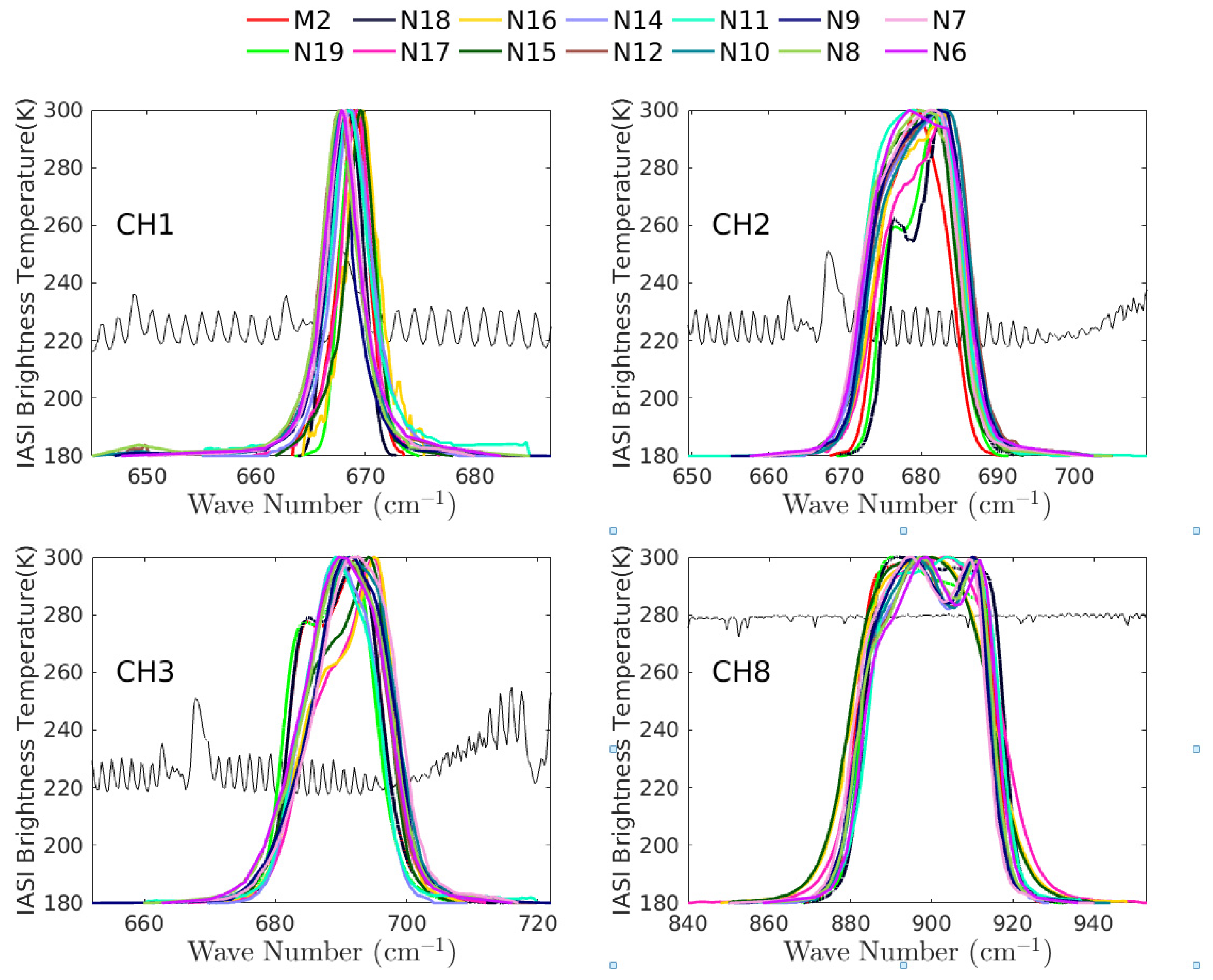
Figure 1 shows the pre-launch measured SRFs for the HIRS channels of interest in this study (Channels 1–3, and 8)—on NOAA-06 to NOAA-19, together with typical IASI-observed brightness temperatures in the background. The center wavenumber (CWN) is derived from the SRF, defined as the wavenumber that splits the area under the SRF into two halves. Table 1 lists the CWNs of these channels on NOAA-06-NOAA-19 and MetOp-A/B. From both Figure 1 and Table 1, the SRFs of HIRS channels show differences among satellites. Inter-satellite CWN differences for the same channel between two HIRS are up to 5 wavenumbers, which is very significant in inter-satellite biases and can significantly affect time-series studies. In addition to the HIRS inter-satellite HIRS SRFdf, there is also SRFerr due to prelaunch measurement uncertainties for each HIRS model as discussed in previous studies [10].
The HIRS intersatellite radiance bias can be expressed as a function of SRF in the following equation:
where is the HIRS inter-satellite radiance bias for channel i on satellite m relative to the same HIRS channel on satellite m + 1, is the HIRS observed radiance for channel i on satellite m, which can be further decomposed into ; is assumed to be the true and accurate radiance value, while Rσ is the radiance bias error term due to SRFerr; is the HIRS radiance for channel i on satellite m + 1 and has already been corrected, SRFdf is the de facto SRF difference between these two satellites, and SRFerr is the SRF measurement error for HIRS on satellite m.
Our goal is to quantify Rσ in Equation (3) so that this error can be corrected through spectral shift related to SRFerr. In Equation (3), we can obtain the at the simultaneous nadir overpass observations between the two satellites, as well as , which has already been corrected (such as HIRS on IASI); however, there are still two unknowns in one equation ( Rσ).
In Chen et al. [8], a radiometric model was introduced to estimate the radiances for a given HIRS SRF based on the correlation between the radiance for a given channel and all other channels.
where =predicted HIRS radiance for channel i on satellite m (as proxy for the true value);; =offset of the HIRS channel radiance on satellite m + 1.
Chen et al. [8] has demonstrated that this radiometric model is accurate enough to predict HIRS radiance for a channel based on all other channels for a given pixel and atmospheric profile. Therefore, Equation (3) can now be rewritten as:
The next step is to minimize Rσ by spectrally shifting the SRF of channel i on satellite m, which will lead to the corrected SRFcor.
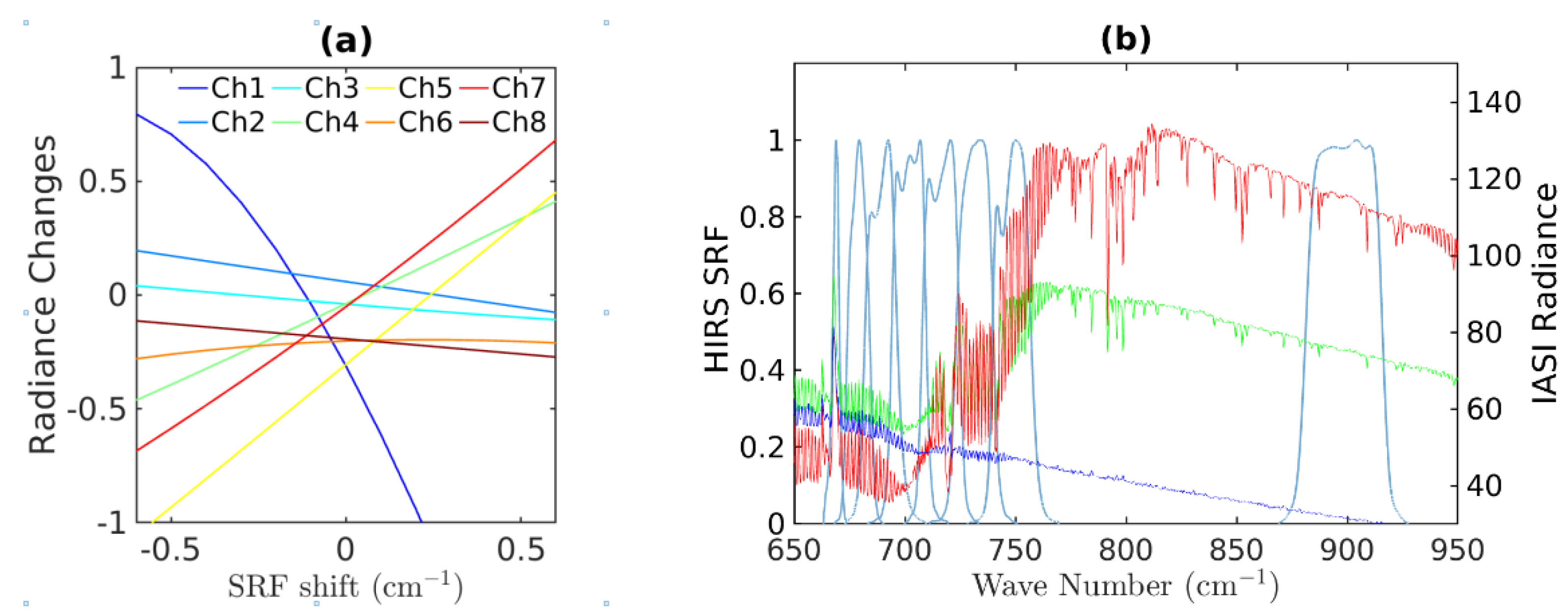
It is noted that while in general, the Chen et al. [8] algorithm is valid, due to the smaller spectral sensitivity of the channels in this study, uncertainties in the SNO time series can overwhelm the expected bias in the time series. Using this method as is without modification may cause large errors for those channels with small sensitivity to SRF shifts. Figure 2 shows the radiance bias sensitivity to the SRF shift. Here, the IASI hyperspectral radiance on MetOp-A is used to convolve with HIRS SRF to calculate the MetOpMetOp-A HIRS radiance and compared with the HIRS observations on the same satellite, similar to the method used in [11]. The largest slope occurs for Channel 1, where bias is negatively correlated with the SRF shift. Cao et al. [9] and Shi et al. [14] have shown that Channel 1 has the biggest inter-satellite bias difference among these channels, which most likely are due to the SRF differences and uncertainties. Other channels usually have much less slope and hence less sensitive to the SRF shift. Nevertheless, a consistent, nearly linear response between the radiance bias and SRF shift exists for all channels, even for Channel 8, which is located in a relatively flat region in the spectral absorption curve, but on the slope of the Planck function curve near 11 um.
The SNO methodology has been well documented in previous studies and will not be discussed in detail here [8,9,11]. It should be noted that caution must be taken when dealing with channels with small/weak sensitivity to SRF shift and where the radiance spatial variance is large over the SNO area. A stricter criterion of the SNO time series has been used for this purpose compared to the Chen et al. [8] SNO time series. In Chen et al. [8], the SNO time series is constructed by averaging data over a ‘square’ area with adjacent 10 along-track rows and 10 along-scan columns near the SNO locations. They found that shifting the start of the scan line can slightly change the SNO results. Nevertheless, it is good enough for comparison for the Channels of 4, 5, and 7 due to its large spectral sensitivity. However, for channels with smaller spectral sensitivity, such as Channels 1–3, and 8, a SNO time series with less variation is needed. In this study, we reconstructed the SNO time series using a different approach (with stricter criteria) so that the SNO time-series standard deviation is remarkably reduced compared to the previous study. First, the true SNO pixels (intersection of the two satellite tracks within a 5-min interval) are located. Then, we search for those field of view (FOV) pairs that are less than 5 km apart within a radius of 500 km. The radiance values over those paired FOVs for each satellite are then averaged, respectively. The radiance ratio (normalized by the later satellite radiance) is always used consistently for analysis in this study. Similar to previous studies, we separate the SNO time series into the North and South Polar regions. All processes are based on both time series, respectively, and final results are then averaged.
3. Results and Discussion
3.1. HIRS on MetOp Satellites
As discussed in the previous section, all HIRS SRFs need to be corrected relative to MetOp IASI eventually. The first step is to correct MetOpMetOp HIRS SRF and then propagate backward to other satellites so that the final SRF shift between each satellite pairs are referenced to MetOp-A IASI. The MetOp-A HIRS SRF shift relative to MetOp-A IASI has been calculated using a similar method as in [11]. We used data from 03/01/2014 for MetOp-A IASI. Table 2 lists the SRF shift of the eight channels between HIRS and IASI over MetOp-A. Note that this SRF shift is relatively small, indicating the high quality of HIRS onboard MetOp-A. The results are consistent with those in [11] for the calculated channels. Since IASI on MetOp-B and MetOp-A are both well-calibrated within 0.1 K [15], we also used the MetOp-B IASI to check the SRF shift for MetOp-B HIRS. The results are also presented in Table 2. However, a large deviation is found for Channel 4 with about a 1.2 cm−1 shift. This has been reported in a previous HIRS study [1]. With the HIRS SRF on MetOp-A spectrally recalibrated, now the rest of the effort focuses on HIRS on earlier satellites. This is primarily done through inter-satellite calibration at the SNOs, and later also uses global means for satellites without SNOs.
3.2. HIRS on NOAA Satellites
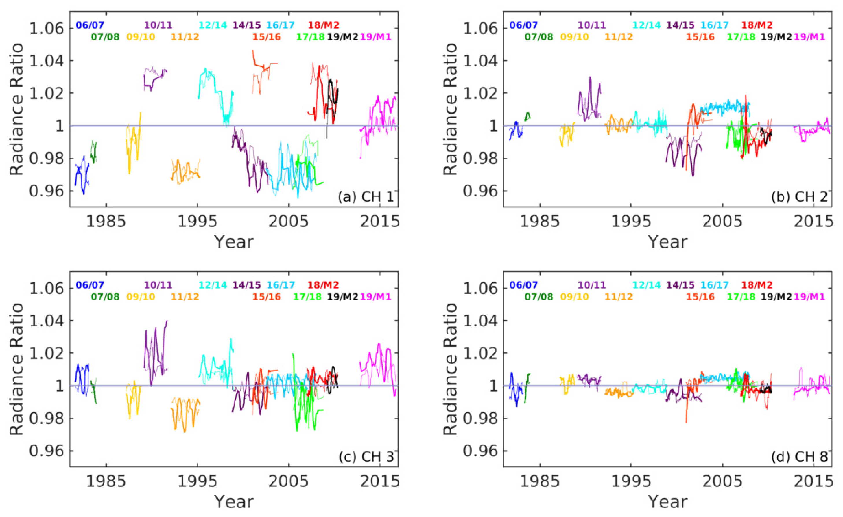
The time series of radiance ratio over SNOs for the channels studied show clear biases among different satellites (Figure 3).
Here, the radiance ratio is defined as the ratio of the HIRS channel radiances from earlier satellites divided by that of the later (successor) satellite at the SNOs for a matching pair of satellites. Among all those channels studied, Channel 8 (the atmospheric window channel) has the smallest inter-satellite bias, generally less than 0.5% in radiance, although the inter-satellite difference can be seen clearly from the figure and are different from one satellite pair to another. These biases are generally higher than the bias for HIRS on MetOp-A relative to IASI. In contrast, Channel 1 has the largest inter-satellite bias, more than 4% for some satellite pairs (e.g., NOAA-15/NOAA-16), with consistent North/South hemisphere differences. This large bias has been reported in several previous studies [9,14]. Most of the satellite pairs have a consistent correlation between the HIRS de facto SRF CWN difference (SRFdf) and radiometric biases. The positive correlation between them suggests that the biases can mostly be explained by SRFdf, while the negative correlation for a few pairs (especially for those with small CWN differences such as NOAA-09/NOAA-10) is likely due to SRF errors (SRFerr) caused by prelaunch measurement uncertainties as discussed earlier. These features are consistent with previous analyses done by [9,14]. By shifting the SRF to the left or right to reduce SRFerr due to the uncertainties, we can find an optimal SRF value at which the radiance difference can be minimized.
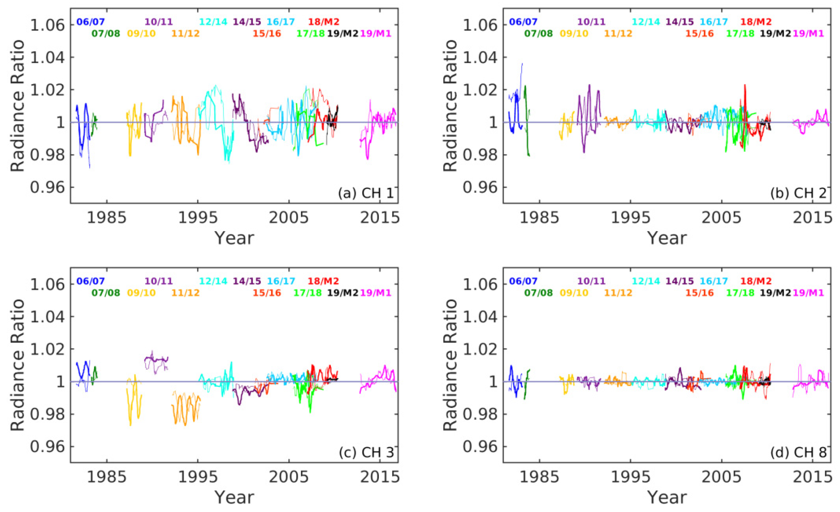
Using Equation (3), the predicted HIRS radiance for a given channel is generated to estimate the radiometric bias due to SRFdf. Figure 4 shows the radiance ratio between the consecutive two satellites for all channels studied after accounting for the effects of the HIRS SRFdf. Indeed, in most cases, the inter-satellite bias has been reduced significantly. For example, the radiance ratio time series of Channels 1, 2, and 8 now are aligned almost to 1. For Channel 3, there are still some residual biases for SNO pairs before the year 2003. The residual bias indicates that there are still biases caused by other factors, which can be attributed to SRFerr or uncertainty. It is also observed that there is very little difference between the bias over the North and South SNO locations, which simplifies the SRFerr correction in the next step.
After accounting for the radiance biases due to SRFdf, the next step is to reduce the residual biases caused by SRFerr due to prelaunch measurement uncertainties. Figure 5 shows the radiance ratio over SNOs after the intermediate SRF correction as described in Equation (5). In this figure, both the HIRS SRFdf and SRFerr due to measurement uncertainty have been removed from the time series. The SRF correction has been referenced to the late satellite in each satellite pair. This method can effectively reduce the bias between the two satellites. Except for Channel 3, the correction works well for almost all channels in the time series (ratio very close to 1). For Channel 8, the ratio biases are within a range of 0.01% (close to 1) with a standard deviation less than 0.04. The corrected South and North Pole biases at SNOS are now very similar and close to each other. For Channel 1, the maximum bias is 0.8% for South Pole SNO between HIRS on NOAA-18 and MetOp-A with a standard deviation of 0.02. For Channel 2, the maximum bias is 0.3% between NOAA-10/NOAA-11 and a standard deviation of 0.01. For Channel 3, the maximum bias is about 1.6% between NOAA-11/NOAA-12 with a standard deviation of 0.005. From the time series, Channels 1–3 are less sensitive to the SRF correction than Channel 8. Further discussions on each channel are provided below.
It is known that HIRS Channel 1 is located at the CO2 Q-branch at the 15 um (or 667 cm−1). Q-branch is where the vibrational transitions occur with the same rotational quantum number (ΔJ = 0) in the ground and excited. In theory, CO2 absorption is very strong at the Q-branch, and a very low radiance is expected. However, as it is shown in the IASI spectrum in Figure 2b, instead, there is an upward spike in radiance at this spectral region. The reason for this spike is not directly due to strong CO2 absorption, but instead because it is sensing a higher layer (upper stratosphere with a HIRS weighting function peak at ~30 hPa) of the atmosphere with a higher temperature at this spectral region, due to the opaqueness with strong CO2 absorption. On the high-frequency side (towards 750 cm−1) of the Q-branch, the energy of rotational transitions is added to the energy of the vibrational transition. This is known as the R-branch of the spectrum for ΔJ = +1, where the rest of the HIRS CO2 channels are located. In contrast, the P-branch for ΔJ = −1 lies on the low wavenumber side of the Q branch, which is not covered by the HIRS channels. The appearance of the R-branch is very similar to the appearance of the pure rotation spectrum, and the P-branch appears as a near mirror image of the R-branch.
Therefore, Channels 1, 2, and 3 are located on the R-branch of the CO2 spectral absorption curve between 13 and 15 um from IASI observations, which is relatively flat, although a slope in radiance is still present as shown in Figure 1, which makes the SRF shift method in Chen et al. [8] still applicable. However, for Channel 3, the relatively flat SRF curve makes the algorithm difficult to converge. When the least-squares method is used, it cannot be minimized towards zero (Figure 5 for Channel 3), though the SRF shift values are reasonably good visually. For Channel 1, after SRF correction, the south-pole and north-pole time series become more different in the final time series. Although the results in the radiance ratio are close to 1, the variability increases as the bias are reduced. Channel 1 also has a nonlinear and sensitive response of radiance bias to SRF shift due to the radiance spike at 667 cm−1, though the SRF shift can account for a large bias reduction. It is also noted that the SNR of Channel 1 is the smallest among all the 12 longwave infrared channels [9], which implies larger radiometric uncertainties.
Overall, while the method works well to reduce inter-satellite bias, there are uncertainties compared to the other CO2 channels studied by Chen et al. [8]. It should be kept in mind that while the time series work better for channels with linear sensitivity in response to SRF shift, for other channels (such as Channel 1), errors can also be propagated from one satellite SRF correction backward and accumulated in the SRF corrections for the earlier satellites. Thus, these spectral shift values have uncertainties, and users must exercise caution for long-term trending studies.
Channel 8 observes the Earth’s surface and is located in a spectrally relatively flat part on the spectral absorption curve. Thus, its sensitivity to SRF shift due to CO2 absorption is small, as shown in Figure 2a. However, the Planck function is nonlinear and dominates this spectral region. As a result, we found that the SRF shift methods work very well to reduce inter-satellite bias. As [11] illustrated, Channel 8 of HIRS onboard, MetOp-A has a bias of about 0.15 K compared to IASI, which can be due to several factors such as nonlinearity blackbody non-unity emissivity, and SRF shift. This study found that the inter-satellite bias before any adjustment can be as high as 0.5% (e.g., NOAA-14/NOAA-15 and NOAA-16/NOAA-17), though this is generally small compared to other channels. This bias has been reduced effectively to be less than 0.01%, and the SRF correction works well for this channel.
3.3. Bridging the Gap between NOAA-07 and NOAA-09 Using the Global Mean Method
The SNO time series allowed us to address the HIRS SRF issues for satellite pairs with SNOs, as presented in previous sections. However, there was a period in history when there were no SNOs in the mid-1980s between NOAA-09 and previous satellites (NOAA-06/07/08). The satellite mission life for NOAA-08 was much shorter by today’s standards. As a result, an alternative method has to be used to bridge this gap. Here, we choose to use the global mean radiance method, primarily because the equator crossings of these two satellites are similar, which significantly reduces the daily cycle effects in the inter-satellite calibration. The concept of the global mean method is not new, and the method has been used previously for climate studies. Here, we focus on correcting the HIRS SRF errors using this method.
NOAA-09 has a valid data period of 25 February 1985 to 14 November 1988, while NOAA-07 has a valid data period of 15 December 1981 to 02 February 1985. Though NOAA-09 has two months of data overlapped with NOAA-07 before 25 February 1985, these data are missing from the NOAA CLASS data archive, and only a few points of SNOs exist. With currently available datasets, both NOAA-07 and NOAA-09 have several years of observations, but no overlap observations. The gap between the NOAA-09 and NOAA-07 is about one month. Here, we use a global mean method to derive our SRF shift based on the radiance time series globally averaged observations for each month and each channel.
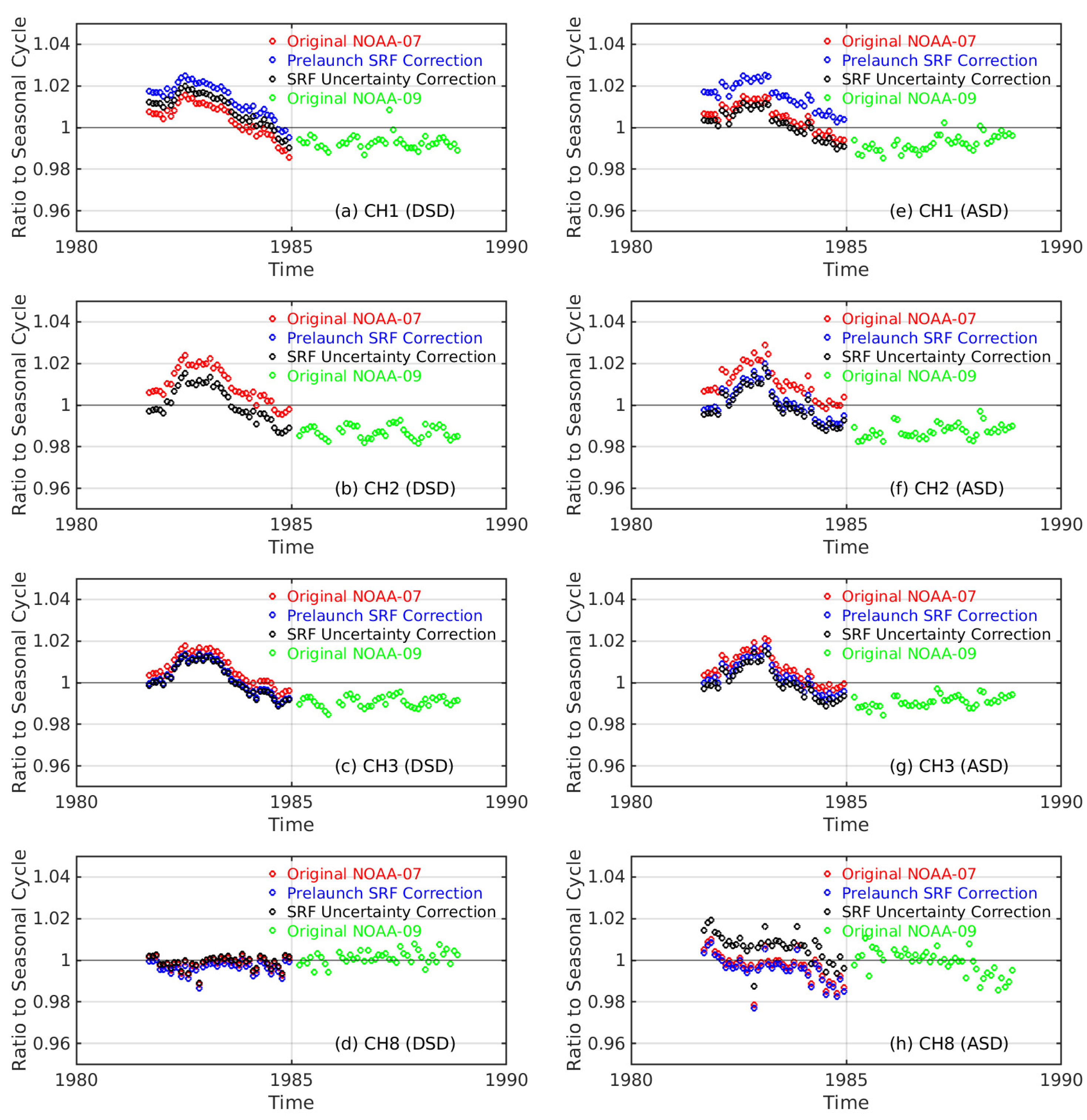
Figure 6 shows the radiance ratio of the global mean radiance normalized by the fitted seasonal cycle. Immediately, the difference between the two satellites can be identified. For example, the ratio of Channel 2 changes from 0.993 on January 1985 of NOAA-07 (last red dots) to 0.985 on March 1985 of NOAA-09 (first green dots). This large jump cannot be explained by climate change compared to the Outgoing Longwave Radiation (OLR) time series. Channels 1–3 have similar patterns for both NOAA-07 and NOAA-09, respectively. It is found that a high monthly anomaly existed in the NOAA-07 radiance time series for Channels 1–3. The highest ratio occurs during 1982–1983, which is a strong El Niño year. These channels have been used to study the OLR [16], and been used to construct the ENSO index [7]. These higher monthly anomalies are consistent with that in the OLR time series. The month-by-month variation is usually small with amplitude less than 0.5%. The abrupt change of the radiance ratio from the last half-year of NOAA-07 and the first half-year of NOAA-09 can only be explained by the SRF difference. For Channel 8, the time series is relatively flat, and the inter-annual variability is small compared to Channels 1–3, usually less than 1.5%.
Note that the difference between descending and ascending time series exists. For example, one can see positive trending for Channel 2 and negative trending for Channel 8 in the NOAA-09 ascending time series (daytime), where the climate signals are relatively flat in the OLR time series. These are caused by the diurnal variation when local crossing time changes with time. For this reason, only nighttime results (descending orbit) are used in the final results because the diurnal changes at night are expected to be much less than those at daytime [17].
With the global mean method, first we look at each month with the HIRS observations over each area grid (0.25 by 0.25) from −80° S to 80° N. Then, the radiance average over each month and each grid is computed and then globally averaged (area-weighted) to get a monthly time series for N07 and N09, respectively, for each channel. We only use HIRS pixels near nadir (from pixel 26–31). Then, the annual and semi-annual signals are fitted and extended to every month for both time series. The time series of radiance ratio (to the seasonal cycle) is analyzed to derive the SRF shift. This global time series method is derived similarly to that used by [18] to study the global daily cycle. For different channels, the responses to the climate signal are different. The long wave infrared channels have been used to monitor the longwave radiation, are very sensitive to the ENSO signals, and have been used as an indicator of ENSO activity. HIRS OLR time series displayed a strong inter-annual variability, especially around 1983 [6,7], though the actual cause of this strong anomaly is still in debate (such as volcano eruption versus ENSO). In minimizing the SRF shift, we only consider the data 6 months before and after February of 1985 to avoid large monthly anomalies. We assume the climate signal does not change during the short non-overlapping period relative to the OLR time series.
Diurnal cycles can cause significant difference when two satellites observe the earth at different local times [18,19] and can be propagated into the climate signal. This diurnal effect must be taken into account. Fortunately, NOAA-07 and NOAA-09 are both in the afternoon orbit, and their equatorial crossing times are very close to each other when launched (both at 14:30, see Figure 1 in [19]). However, the equator crossing time drifted about 1 h during their lifetime for both satellites. We consider only time series for descending orbit (most observations are at night, with beginning equator crossing time at 2:30 AM).
Similar to the SNO method, we define a model to simulate the radiance bias and hence derive the optimal SRF shift (intermediate between NOAA-09 and NOAA-07) for each channel. The correction has been also separated into two steps: HIRS SRFdf, and SRFerr due to uncertainties for each satellite.
The first step is to quantify the bias due to HIRS SRFdf between NOAA-07 and NOAA-09. However, the least-squares fitting cannot be directly applied to the global mean time series, especially for Channel 8 and other channels with small spectral sensitivity. The radiance seasonal cycle amplitude of Channel 8 (76–81 mW/(m2 sr cm−1)) in the global mean time series is much less than the actual radiance range (15–150 mW/(m2 sr cm−1)) observed. In contrast, the averaged global radiance is close to the onboard blackbody radiance. At that point, the SRF shift induced radiance change approaches zero. If the global mean values are directly used, the least-squares can cause algorithm singularity and thus a very large unrealistic SRF shift. Therefore, we have to address the HIRS SRFdf effect using the original HIRS datasets directly instead of using the global mean at this step.
On the other hand, the inter-channel dependency shown in Equation (3) changes with time and location. In Chen et al. [8], the inter-channel dependency is derived using only high latitude IASI data since SNOs occur only in the polar area. Before deriving the radiance corrections due to the HIRS SRFdf, we first derived the latitude-dependent inter-channel coefficient. To consider HIRS SRFdf, the coefficient W and C in Equation (4) is derived using the IASI observations in each zone with a 2.5° interval from −80° S to 80° N. In each zone, we first simulate the HIRS (of NOAA-07) using IASI data for January 2014. Consistent with HIRS nadir data, only those data over IASI pixels near the nadir have been used. Then, we use Equation (4) to calculate a set of coefficients specific to that latitude zone through the leasts-squares fitting. These coefficients are then applied to the original HIRS datasets (using Equation (3)) to address the radiance bias caused by the HIRS SRFdf between satellites and then a globally averaging is carried out to form a new time series compared with the original global mean time series without HIRS SRF corrections. By doing so, we have accounted for the latitude dependency of the inter-channel correlations. The newly obtained time series has removed the HIRS SRFdf effect between NOAA-07 and NOAA-09. Note that the data processing of global HIRS and IASI observations is computational intensive and requires many CPU hours, a supercomputer with an embarrassingly parallel scheme (https://en.wikipedia.org/wiki/Embarrassingly_parallel, accessed on 10 July 2021) has been used for this study.
The next step is to reduce the residual radiance bias through SRF shift to correct the HIRS SRFerr. Similar to the SNO method, SRF shift is performed as discussed earlier. With SNO overlapping, the comparison is made between two time series over the same period. However, here we assume the jumps and discrepancies in the radiances between NOAA-07 and NOAA-09 global mean time series are solely caused by the SRFerr due to uncertainties. To reduce the inter-annual “climate change” effects, we only look at the time series within one year period near the breakpoint (February 1985). We assume that the global mean time series of the pre-six-month period (NOAA-07) and after six months (NOAA-09) should yield the same mean values if there are no SRF differences. Thus, we can compare the NOAA-07 ratio from different SRF shifts, and the NOAA-09 mean ratio (over the post six-month period) to derive the optimal SRF shift.
In the second step, to simulate the HIRS radiance with IASI to obtain the coefficients to determine SRF error in Equation (3), we shifted the SRF between −4.0 cm−1 to 4.0 cm−1 with an interval of 0.2 cm−1 relative to the NOAA-07 CWN of each channel and convolved with IASI hyperspectral radiances. Thus, using the simulated HIRS data from IASI over one month globally (January 2014), 41 sets of coefficients (latitude dependent) can also be derived for each latitude zone using Equation (4). These coefficients are then applied to HIRS observations (NOAA-07) and averaged globally. Then, we have 41 sets of global mean radiance time series. After normalizing the time series using the same seasonal cycle, we compared the mean absolute difference between each time series of NOAA-07 to the mean of the NOAA-09 (no SRF shift) for each channel. The optimal SRF is determined between NOAA-07 and NOAA-09 when the error approaches the minimum among 41 comparisons in Equation (5). As a result, from NOAA-06 to MetOp, we have obtained corrected HIRS SRF for each pair of satellites.
Figure 6 shows the HIRS SRFdf effect between satellites on each channel (blue line), especially Channel 2 from the descending orbit time series. It also shows the time series after SRF error correction (black line) described in Section 2. Immediately, one can see the two time series become aligned closely near Feb. 1985 after the optimal SRF shift has been applied to NOAA-07. Thus, the optimal SRF shift (of the satellite pair) can then be used to bridge the gap between NOAA-09 and NOAA-07 with the optimal radiance correction in the absence of SNO.
For each satellite pair, the SRF shift (intermediate SRF shift) was obtained in reference to the later satellite in the pair. The next step is to reference the SRF shift to MetOp-A IASI as done in Chen et al. [8].
3.4. Connecting the 40+ Year HIRS Time Series with Final SRF Correction
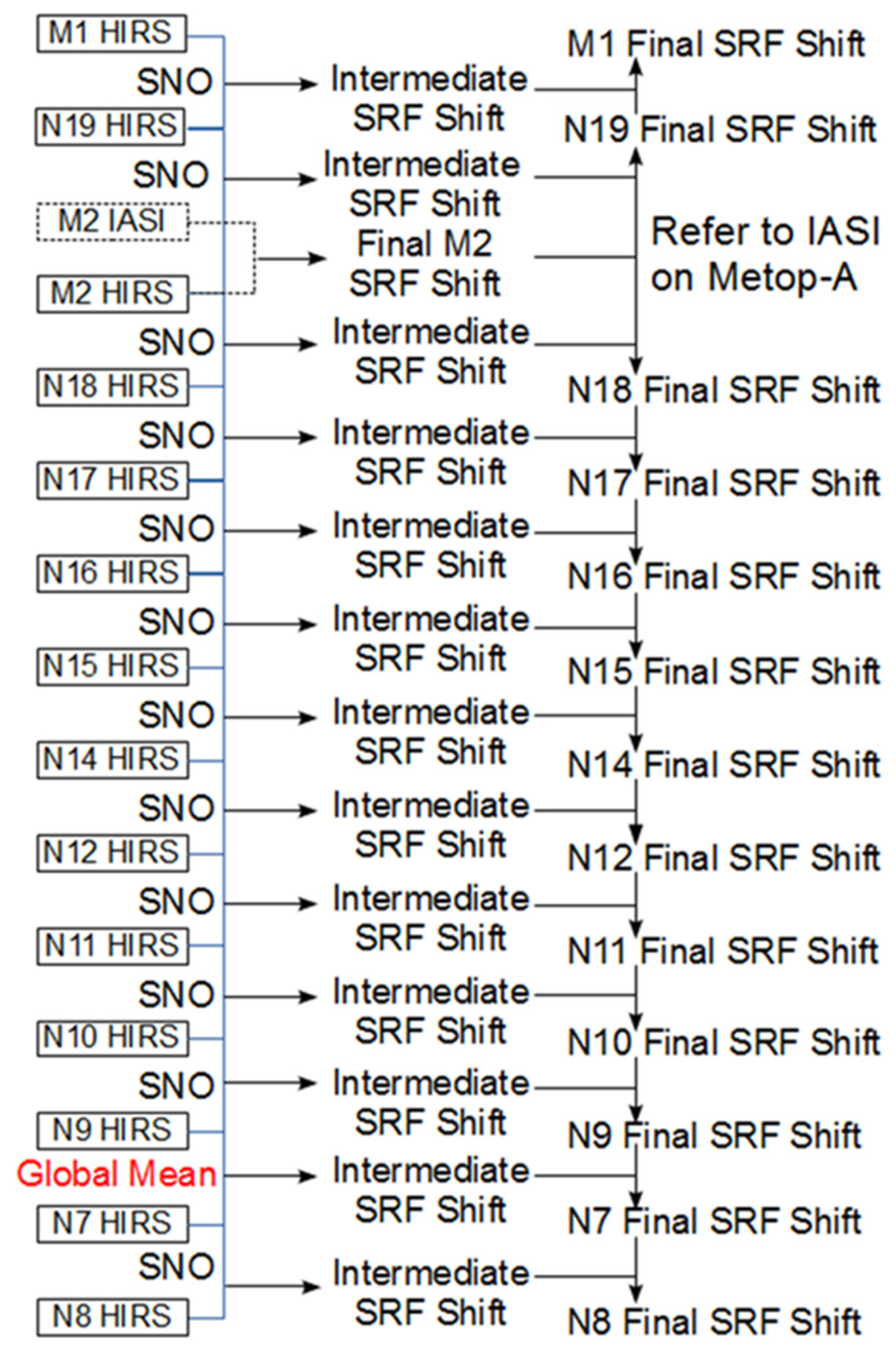
The same method in Chen et al. [8] is used to propagate the SRF shift from MetOp-A HIRS to earlier and later satellites (NOAA-19/MetOp-B). Scheme 1 shows the flow chart of how the SRF propagation was done schematically. We start from the MetOp-A IASI and HIRS comparison (on the same satellite) to derive the MetOp-A HIRS SRF shifts relative to MetOp-A IASI. We then propagate the comparison back to earlier satellites one by one from Metp-A HIRS to NOAA-19, to NOAA-18, and back to NOAA-9. Then, the global mean method was used to bridge the gap between NOAA-9 and NOAA07, which allows us to connect back to NOAA-06. The final SRF shift is then determined for each satellite and each channel, now referred to as MetOp-A IASI. An equation for this has been used for propagating the SRF corrections.
is the final SRF shift relative to the pre-launch SRF (); is an optimized central wavenumber for that channel at satellite n; is the intermediate SRF correction (SRFdf and SRFerr). The SRF calculations are separated into the South and North pole, and the final SRF shifts are calculated as the mean values between the North and South poles when the SNO method is used, while the global mean yields only one value using descending orbit dataset. The final optimized SRF shift () for each channel of these satellites are given in Table 2.
The HIRS SRF error correction may have significant impacts on climate studies. For global climate studies, such as the OLR time series [6,16], the subtraction of the global mean radiance bias over the overlapping period after diurnal correction appears to be a straightforward method. However, in other applications, such as climate study using the derived products from HIRS (such as clouds, water vapor time series [1]), the corrected SRFs will be used to recalculate the coverage of clouds in a radiative transfer model, and therefore it becomes important. Radiative transfer models and atmospheric retrievals often use SRF to calculate the coefficients and atmosphere transmittance coefficients. Errors in SRF can propagate into the forward model, tangent linear and adjoint models through these coefficient calculations, affecting the accuracy of the retrieval products [20].
4. Conclusions and Future Work
In this study, we further verified and extended the HIRS SRF re-calibration work of Chen et al. [8] (Channel 4, 5, 6, and 7) to other HIRS long-wave infrared channels (Channels 1, 2, 3, and 8) sensing the upper stratosphere and surface, using a similar SNO method as used previously. We further bridged the gap between NOAA-09 and NOAA-07 in the time series using the global mean method due to the lack of SNOs between these two satellites. In addition, MetOp-B HIRS SRF is also recalibrated with MetOp-B IASI. The effects of HIRS de facto SRF difference between each satellite pair are quantified to reduce the inter-satellite radiometric biases. The residual bias is then reduced through SRF error correction by shifting the SRF within the uncertainty. The final SRF shift referenced to MetOp IASI is then calculated through backward propagation of the SRF correction from MetOp-A HIRS to NOAA-06. The SRF shift can effectively reduce the inter-satellite bias in the HIRS observations of the same channels in the time series. On the other hand, the HIRS SRF correction for Channel 3 may have larger uncertainties because of its weak relationship between SRF shift and radiance bias, and Channel 1 appears to have a nonlinear relationship between SRF shift and bias since it sits on a spike of the Q-branch of the CO2 absorption sensing the upper stratosphere. Therefore, users should exercise caution when using the recommended SRF shift values for Channels 1 and 3.
It is understood that satellite instrument characteristics may change over time and it can be very difficult to quantify some of the changes (such as the shape of the spectral response functions). As a result, this study extended a previous published algorithm, and also inherits some of the uncertainties. Ideally, the satellite instrument at the end of the mission life should be brought down to the earth and reanalyzed in the laboratory to quantify the instrument changes. Unfortunately, this is not possible for most missions. As a result, the uncertainties from the previous algorithm and assumptions remain and need to be further studied.
On the other hand, based on our analysis and previous studies of instrument characteristics, we believe that the two major factors affecting the HIRS intersatellite biases are in the SRF differences between instrument models and SRF measurement uncertainties. The SRF shape is largely determined by the materials, space between the layers, and incident angle of the interference filters mounted on HIRS filter wheel, while the onboard blackbody emissivity is largely determined by the honeycomb structure, which does not change over time. Nevertheless, the assumptions in these parameters may not be entirely accurate, but instead are the best estimates based on the current knowledge. We hope that in the future, there may be better ways to quantify instrument changes over satellite mission life. The upcoming benchmark missions may also help to reduce the uncertainties as well, which will present new opportunities for future studies. Additionally, compared to the previous method used by [11], the SRF shift method in this paper does not take into account the calibration nonlinearity effect, since the nonlinearity effect is generally much smaller than SRF induced uncertainties due to the fact that that the instrument self-emission dominates the radiation on the detector while the incoming varying signal is only a very small portion of the total radiation falling on the detector, thus detector nonlinearity effect is not significant [21]. The errors in the derived optimal SRF may manifest on the radiance time series to cause the time series coherency and power spectra changes as discussed for ENSO in [22]. A wavelet method [22,23] can be used to determine this in the future.
Author Contributions
Software, T.-C.L., B.Z.; validation, T.-C.L., X.S. and B.Z.; formal analysis, B.Z.; investigation, B.Z.; resources, X.S.; data curation, X.S., T.-C.L. and B.Z.; writing—original draft preparation, B.Z.; writing—review and editing, C.C., B.Z. and X.S.; visualization, T.-C.L. and B.Z.; supervision, X.S. and B.Z.; project administration, X.S.; funding acquisition, X.S. All authors have read and agreed to the published version of the manuscript.
Funding
This study was partially supported by NOAA grant NA19NES4320002 (Cooperative Institute for Satellite Earth System Studies—CISESS) at the University of Maryland/ESSIC. This research was partially funded by NOAA NCEI, in collaboration with University of Wisconsin.
Institutional Review Board Statement
Not applicable.
Informed Consent Statement
Not applicable.
Data Availability Statement
The HIRS and IASI data used for this study are available at NOAA CLASS: https://www.avl.class.noaa.gov/saa/products/welcome, accessed on 10 July 2021.
Acknowledgments
This study was conducted under NOAA NCEI funding to the astronomy department, University of Maryland, College Park. The scientific results and conclusions, as well as any views or opinions expressed herein, are those of the author(s) and do not necessarily reflect those of NOAA or the Department of Commerce. The authors thank Paul Menzel at the University of Wisconsin for initiating and supporting this project. We also thank Shu-peng Ho at NOAA STAR for his valuable comments on this paper.
Conflicts of Interest
The authors declare no conflict of interest.
Abbreviations
| HIRS | High resolution Infrared Radiation Sounder |
| NOAA | National Oceanic and Atmospheric Administration |
| MetOp | Meteorological Operational satellite |
| OLR | Outgoing Longwave Radiation |
| ENSO | El Niño-Southern Oscillation |
| SRF | Spectral Response Function |
| SNO | Simultaneous Nadir Overpasses |
| WMO | World Meteorological Organization |
| GCOS | Global Climate Observing System |
| IASI | Infrared Atmospheric Sounding Interferometer |
| MATLAB | Matrix Laboratory software |
| IDL | Interactive Data Language |
| BEAT | Basic Envisat Atmospheric Toolbox |
| CODA | Common Data Access Toolbox |
| NESDIS | National Environmental Satellite, Data, and Information Service |
| STAR | Center for Satellite Applications and Research |
| CWN | Central Wavenumber |
| NCEI | National Centers for Environmental Information |
References
- Menzel, W.P.; Frey, R.A.; Borbas, E.E.; Baum, B.A.; Cureton, G.; Bearson, N. Reprocessing of HIRS Satellite Measurements from 1980 to 2015: Development toward a Consistent Decadal Cloud Record. J. Appl. Meteor. Climatol. 2016, 55, 2397–2410. [Google Scholar] [CrossRef]
- Wylie, D.P.; Menzel, W.P. Eight Years of High Cloud Statistics Using HIRS. J. Clim. 1999, 12, 170–184. [Google Scholar] [CrossRef]
- Wylie, D.; Jackson, D.L.; Menzel, W.P.; Bates, J.J. Trends in Global Cloud Cover in Two Decades of HIRS Observations. J. Clim. 2005, 18, 3021–3031. [Google Scholar] [CrossRef]
- Shi, L.; Schreck, C.J., III; John, V.O. HIRS channel 12 brightness temperature dataset and its correlations with major climate indices. Atmos. Chem. Phys. 2013, 13, 6907–6920. [Google Scholar] [CrossRef] [Green Version]
- Shi, L.; Bates, J.J. Three decades of intersatellite-calibrated High-Resolution Infrared Radiation Sounder upper tropospheric water vapor. J. Geophys. Res. 2011, 116, D04108. [Google Scholar] [CrossRef]
- Lee, H.-T. Outgoing Longwave Radiation—Monthly Climate Data Record Algorithm Theoretical Basis Document. NOAA/NCDC Rep. 2014. Available online: https://www1.ncdc.noaa.gov/pub/data/sds/cdr/CDRs/Outgoing%20Longwave%20Radiation%20-%20Monthly/AlgorithmDescription_01B-06.pdf (accessed on 10 July 2021).
- Chiodi, A.M.; Harrison, D.E. Global Seasonal Precipitation Anomalies Robustly Associated with El Niño and La Niña Events—An OLR Perspective. J. Clim. 2015, 28, 6133–6159. [Google Scholar] [CrossRef] [Green Version]
- Chen, R.; Cao, C.; Menzel, W.P. Intersatellite calibration of NOAA HIRS CO2 channels for climate studies. J. Geophys. Res. 2013, 118, 5190–5203. [Google Scholar] [CrossRef]
- Cao, C.; Xu, H.; Sullivan, J.; McMillin, L.; Ciren, P.; Hou, Y. Intersatellite Radiance Biases for the High-Resolution Infrared Radiation Sounders (HIRS) on boardNOAA-15, -16, and -17 from Simultaneous Nadir Observations. J. Atmos. Ocean. Technol. 2005, 22, 381–395. [Google Scholar] [CrossRef]
- Cao, C.; Goldberg, M.; Wang, L. Spectral Bias Estimation of Historical HIRS Using IASI Observations for Improved Fundamental Climate Data Records. J. Atmos. Ocean. Technol. 2009, 26, 1378–1387. [Google Scholar] [CrossRef]
- Chen, R.; Cao, C. Physical analysis and recalibration of MetOp HIRS using IASI for cloud studies. J. Geophys. Res. 2012, 117, D03103. [Google Scholar] [CrossRef] [Green Version]
- Cao, C.; Weinreb, M.; Kaplan, S. Verification of the HIRS Spectral Response Functions for More Accurate Atmospheric Sounding. In Proceedings of the CALCON Meeting, Logan, UT, USA, 23–26 August 2004. [Google Scholar]
- Ohring, G. (Ed.) Achieving Satellite Instrument Calibration for Climate Change (ASIC3); NPOESS Workshop Report, 144; 2007; p. 37. Available online: https://www.nist.gov/system/files/documents/2017/03/15/asic3.pdf (accessed on 10 July 2021).
- Shi, L.; Bates, J.J.; Cao, C. Scene Radiance–Dependent Intersatellite Biases of HIRS Longwave Channels. J. Atmos. Oceanic Technol. 2008, 25, 2219–2229. [Google Scholar] [CrossRef]
- Cameron, J.; Cotton, J.; Marriott, R. METOP-B IASI Data Quality and Impact Assessment. Available online: https://www-cdn.eumetsat.int/files/2020-04/pdf_conf_p_s8_03_cameron_v.pdf (accessed on 10 July 2021).
- Lee, H.; Gruber, A.; Ellingson, R.G.; Laszlo, I. Development of the HIRS Outgoing Longwave Radiation Climate Dataset. J. Atmos. Ocean. Technol. 2007, 24, 2029–2047. [Google Scholar] [CrossRef] [Green Version]
- MacKenzie, I.A.; Tett, S.F.; Lindfors, A.V. Climate Model–Simulated Diurnal Cycles in HIRS Clear-Sky Brightness Temperatures. J. Clim. 2012, 25, 5845–5863. [Google Scholar] [CrossRef] [Green Version]
- Lindfors, A.V.; Mackenzie, I.A.; Tett, S.F.; Shi, L. Climatological Diurnal Cycles in Clear-Sky Brightness Temperatures from the High-Resolution Infrared Radiation Sounder (HIRS). J. Atmos. Ocean. Technol. 2011, 28, 1199–1205. [Google Scholar] [CrossRef] [Green Version]
- Jackson, D.L.; Soden, B.J. Detection and Correction of Diurnal Sampling Bias in HIRS/2 Brightness Temperatures. J. Atmos. Ocean. Technol. 2007, 24, 1425–1438. [Google Scholar] [CrossRef]
- Chen, Y.; Han, Y.; Weng, F. Comparison of two transmittance algorithms in the community radiative transfer model: Application to AVHRR. J. Geophys. Res. 2012, 117, D06206. [Google Scholar] [CrossRef] [Green Version]
- Cao, C.; Jarva, K.; Ciren, P. An Improved Algorithm for the Operational Calibration of the High-Resolution Infrared Radiation Sounder. J. Atmos. Ocean. Technol. 2007, 24, 169–181. [Google Scholar] [CrossRef]
- Torrence, C.; Compo, G.P. A Practical Guide to Wavelet Analysis. Bull. Am. Meteorol. Soc. 1998, 79, 61–78. [Google Scholar] [CrossRef] [Green Version]
- Ghaderpour, E.; Pagiatakis, S.D. LSWAVE: A MATLAB software for the least-squares wavelet and cross-wavelet analyses. GPS Solut. 2019, 23, 50. [Google Scholar] [CrossRef]
Figure 1.
Spectra response function is different from satellite to satellite for the same channel.

Figure 2.
Simulated HIRS radiance changes (relative to IASI observations) sensitive to the channel SRF shift. The left panel (a) shows SRF shift sensitivity. The right panel (b) shows CH 1–8 SRF overlapped with three IASI observations at Desert (Red), SNO (Green), and Polar region (Blue).
Figure 2.
Simulated HIRS radiance changes (relative to IASI observations) sensitive to the channel SRF shift. The left panel (a) shows SRF shift sensitivity. The right panel (b) shows CH 1–8 SRF overlapped with three IASI observations at Desert (Red), SNO (Green), and Polar region (Blue).

Figure 3.
Time series of inter-satellite biases of HIRS 1–3 and 8 channels for NOAA-06 to NOAA-19. Thick lines represent SNO comparisons in the south polar region; thin lines represent SNO comparisons in the north polar region.
Figure 3.
Time series of inter-satellite biases of HIRS 1–3 and 8 channels for NOAA-06 to NOAA-19. Thick lines represent SNO comparisons in the south polar region; thin lines represent SNO comparisons in the north polar region.

Figure 4.
SNO time series of the radiance ratio between two adjacent satellites with prelaunch SRF difference correction.
Figure 4.
SNO time series of the radiance ratio between two adjacent satellites with prelaunch SRF difference correction.

Figure 5.
SNO time series of the radiance ratio between two adjacent satellites with SRF uncertainty correction.
Figure 5.
SNO time series of the radiance ratio between two adjacent satellites with SRF uncertainty correction.

Figure 6.
The global mean method shows radiance ratio time series normalized using seasonal cycle for Channels 1–3 and 8. The green dots represent NOAA-09, the red dots are for the original NOAA-07, the blue dots are after pre-launch SRF correction, and the black dots are after SRF uncertainty correction. The left panels are for descending time (night) and the right panels are for ascending (day) time.

Scheme 1.
Flow chart for SRF final corrections process from intermediate SRF corrections and using IASI as references.
Scheme 1.
Flow chart for SRF final corrections process from intermediate SRF corrections and using IASI as references.


Table 1.
Central wavenumber (unit: 1/cm) for different channels on each satellite.
| SAT | CH1 | CH2 | CH3 | CH4 | CH5 | CH6 | CH7 | CH8 |
|---|---|---|---|---|---|---|---|---|
| M1 | 668.83 | 679.28 | 690.37 | 703.08 | 714.94 | 731.45 | 747.36 | 898.80 |
| M2 | 668.66 | 679.18 | 689.70 | 701.99 | 716.47 | 731.71 | 748.82 | 898.59 |
| N19 | 669.33 | 680.31 | 688.85 | 702.64 | 715.80 | 733.39 | 749.12 | 899.46 |
| N18 | 668.18 | 680.94 | 689.68 | 703.81 | 714.34 | 731.54 | 750.55 | 900.46 |
| N17 | 668.86 | 679.95 | 691.41 | 702.73 | 715.70 | 731.82 | 748.04 | 899.90 |
| N16 | 669.63 | 679.62 | 691.34 | 701.21 | 715.97 | 731.47 | 748.81 | 894.57 |
| N15 | 669.08 | 678.79 | 690.45 | 703.15 | 715.92 | 731.71 | 747.65 | 897.36 |
| N14 | 668.90 | 679.36 | 689.62 | 703.56 | 714.50 | 732.27 | 749.64 | 898.66 |
| N12 | 667.59 | 680.18 | 690.01 | 704.21 | 716.31 | 732.80 | 751.91 | 900.45 |
| N11 | 668.98 | 678.89 | 689.70 | 703.24 | 716.83 | 732.11 | 749.48 | 900.51 |
| N10 | 667.70 | 680.23 | 691.15 | 704.33 | 716.3 | 733.13 | 750.71 | 899.49 |
| N09 | 667.67 | 679.84 | 691.46 | 703.37 | 717.16 | 732.64 | 749.48 | 898.52 |
| N08 | 667.41 | 679.41 | 690.89 | 702.97 | 717.56 | 732.97 | 747.90 | 901.07 |
| N07 | 667.93 | 679.20 | 691.56 | 704.63 | 717.05 | 733.20 | 749.20 | 898.93 |
| N06 | 668.03 | 679.93 | 690.43 | 704.69 | 717.43 | 732.47 | 748.49 | 900.63 |
M1 represents MetOp-B, M2 represents MetOp-A.
Table 2.
Final SRF shift values (relative to MetOp/M2-IASI).
| CH#1 | CH #2 | CH #3 | CH#4 | CH#5 | CH#7 | CH #8 | |
|---|---|---|---|---|---|---|---|
| N6 HIRS/M2I | 4.27 | −3.45 | −0.13 | 0.31 | 0.7 | 0.7 | −3.19 |
| N7 HIRS/M2I | 3.87 | −2.7 | 1.02 | −0.18 | 0.1 | 1.2 | 0.51 |
| N9 HIRS/M2I | 4.10 | −2.66 | 1.18 | 0.43 * | 2.66 * | −0.48 * | 1.58 |
| N10 HIRS/M2I | 4.75 | −3.06 | 0.18 | 0.95 * | 1.56 * | −0.93 * | 1.83 |
| N11 HIRS/M2I | 4.30 | −0.06 | 0.43 | 1.72 * | 2.05 * | 0.15 * | 1.38 |
| N12 HIRS/M2I | 1.85 | −0.71 | -0.37 | 0.47 * | 2.23 * | −2.06 * | 1.08 |
| N14 HIRS/M2I | −0.25 | 0.79 | 0.63 | 1.97 * | 3.13 * | 1.22 * | 0.68 |
| N15 HIRS/M2I | −1.40 | −0.46 | −1.17 | −0.21 * | 0.27 * | 1.01 * | −0.62 |
| N16 HIRS/M2I | −0.50 | −0.31 | −0.97 | 0.22 * | 0.62 * | 0.47 * | −0.42 |
| N17 HIRS/M2I | −0.70 | 1.69 | −0.52 | 0.54 * | 0.72 * | 0.44 * | −0.87 |
| N18 HIRS/M2I | −0.60 | −0.51 | −0.62 | −0.71 * | −0.37 * | −0.49 * | −0.97 |
| N19 HIRS/M2I | −0.55 | 0.64 | −0.42 | −0.00 * | −0.12 * | 0.10 * | −0.47 |
| M2 HIRS/M2I | −0.10 | 0.19 | −0.17 | −0.15 * | 0.10 * | −0.15 * | −0.52 |
| M1 HIRS/M2I | −0.55 | 1.54 | 0.53 | −1.21 | −0.43 | −0.54 | −0.07 |
* Chen et al., 2013 [8].
Publisher’s Note: MDPI stays neutral with regard to jurisdictional claims in published maps and institutional affiliations. |
© 2021 by the authors. Licensee MDPI, Basel, Switzerland. This article is an open access article distributed under the terms and conditions of the Creative Commons Attribution (CC BY) license (https://creativecommons.org/licenses/by/4.0/).
Share and Cite
MDPI and ACS Style
Zhang, B.; Cao, C.; Liu, T.-C.; Shao, X. Spectral Recalibration of NOAA HIRS Longwave CO2 Channels toward a 40+ Year Time Series for Climate Studies. Atmosphere 2021, 12, 1317. https://0-doi-org.brum.beds.ac.uk/10.3390/atmos12101317
AMA Style
Zhang B, Cao C, Liu T-C, Shao X. Spectral Recalibration of NOAA HIRS Longwave CO2 Channels toward a 40+ Year Time Series for Climate Studies. Atmosphere. 2021; 12(10):1317. https://0-doi-org.brum.beds.ac.uk/10.3390/atmos12101317
Chicago/Turabian StyleZhang, Bin, Changyong Cao, Tung-Chang Liu, and Xi Shao. 2021. "Spectral Recalibration of NOAA HIRS Longwave CO2 Channels toward a 40+ Year Time Series for Climate Studies" Atmosphere 12, no. 10: 1317. https://0-doi-org.brum.beds.ac.uk/10.3390/atmos12101317
Note that from the first issue of 2016, this journal uses article numbers instead of page numbers. See further details here.