Article

Generating Flood Hazard Maps Based on an Innovative Spatial Interpolation Methodology for Precipitation

by
Mohammad Zare
1,2,*,
Guy J.-P. Schumann
1,3,
Felix Norman Teferle
2 and
Ruja Mansorian
1
1
Research and Education Department, RSS-Hydro, 100, Route de Volmerange, L-3593 Dudelange, Luxembourg
2
Geodesy and Geospatial Engineering, Department of Engineering, University of Luxembourg, L-1359 Luxembourg, Luxembourg
3
School of Geographical Sciences, University of Bristol, Bristol BS8 1QU, UK
*
Author to whom correspondence should be addressed.
Atmosphere 2021, 12(10), 1336; https://doi.org/10.3390/atmos12101336
Submission received: 15 September 2021 / Revised: 7 October 2021 / Accepted: 10 October 2021 / Published: 13 October 2021

Abstract

:
In this study, a new approach for rainfall spatial interpolation in the Luxembourgian case study is introduced. The method used here is based on a Fuzzy C-Means (FCM) clustering method. In a typical FCM procedure, there are a lot of available data and each data point belongs to a cluster, with a membership degree [0 1]. On the other hand, in our methodology, the center of clusters is determined first and then random data are generated around cluster centers. Therefore, this approach is called inverse FCM (i-FCM). In order to calibrate and validate the new spatial interpolation method, seven rain gauges in Luxembourg, Germany and France (three for calibration and four for validation) with more than 10 years of measured data were used and consequently, the rainfall for ungauged locations was estimated. The results show that the i-FCM method can be applied with acceptable accuracy in validation rain gauges with values for R2 and RMSE of (0.94–0.98) and (9–14 mm), respectively, on a monthly time scale and (0.86–0.89) and (1.67–2 mm) on a daily time scale. In the following, the maximum daily rainfall return periods (10, 25, 50 and 100 years) were calculated using a two-parameter Weibull distribution. Finally, the LISFLOOD FP flood model was used to generate flood hazard maps in Dudelange, Luxembourg with the aim to demonstrate a practical application of the estimated local rainfall return periods in an urban area.

1. Introduction

Changing hydrological conditions, as well as the increasing impervious areas due to increasing urban development, have caused fundamental changes in the surface water regimes (e.g., flood events in recent years) [1]. The magnitude of floods can be estimated by a variety of methods depending on the availability of hydrometric data, more importantly, precipitation data [2,3]. Since it is impossible to install and maintain a rain gauge at every point where data are needed, finding a method to estimate local rainfall is crucial. In recent years, with the development of improved statistical approaches, earth observation technologies and machine learning methods, the accuracy as well as the number of spatial interpolation methods have greatly increased [4,5]. However, in the authors’ opinion, not enough attention has been given to clustering methods and fuzzy logic for spatial interpolation of precipitation; this becomes even more important when thinking meticulously about the process of estimating rainfall data in certain point locations based on measured data around that location. It is clear that in most approaches the process follows the fuzzy concept, i.e., the estimated value of the ungauged point id derived by measured data at other locations, using different weights [6,7]. Spatial interpolation is the process of organizing observed data into groups that are relatively similar, in order to fill the gaps between groups. This type of grouping shows the importance of similarity in interpolation which draws parallels with the concept of clustering and classification. Thus, developing a method that considers fuzziness and clustering approaches at the same time can be an interesting challenge. In this regard, this research introduces an innovative inverse Fuzzy C-Means clustering (i-FCM) method, which has been developed and applied as a spatial interpolation methodology to estimate rainfall data at locations with no measured rainfall, using measured data from nearby locations. Consequently, the widely and successfully applied LISFLOOD-FP flood model will be used to simulate flood events with different daily rainfall return periods (10, 25, 50 and 100) in Dudelange, southern Luxembourg (ungauged location).

2. Materials and Methods

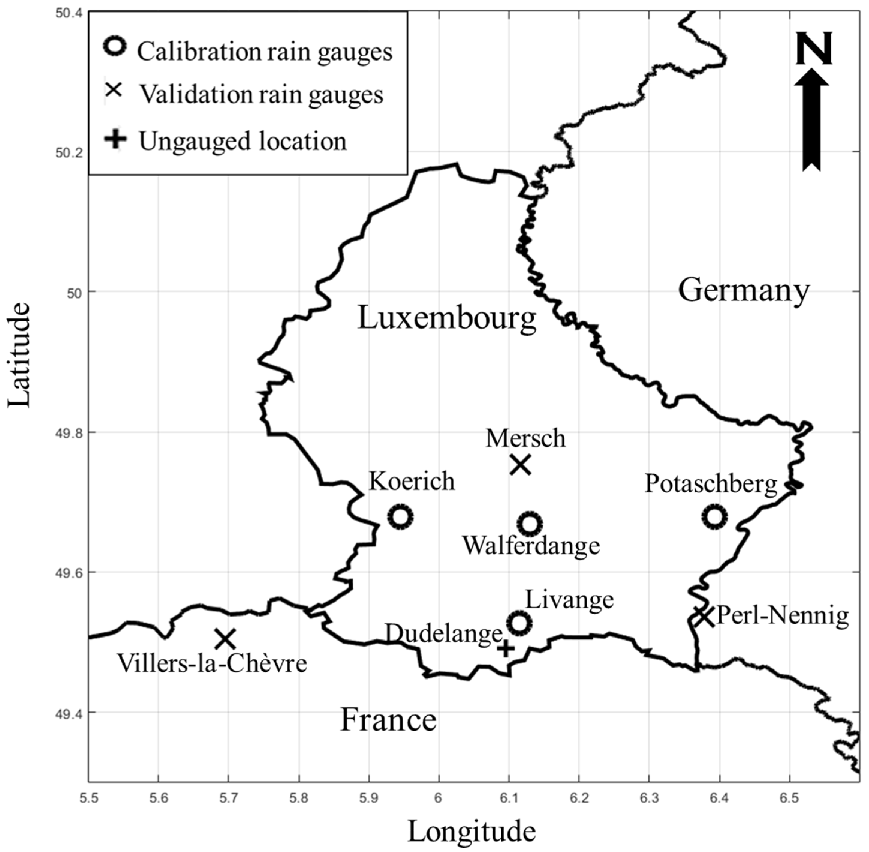
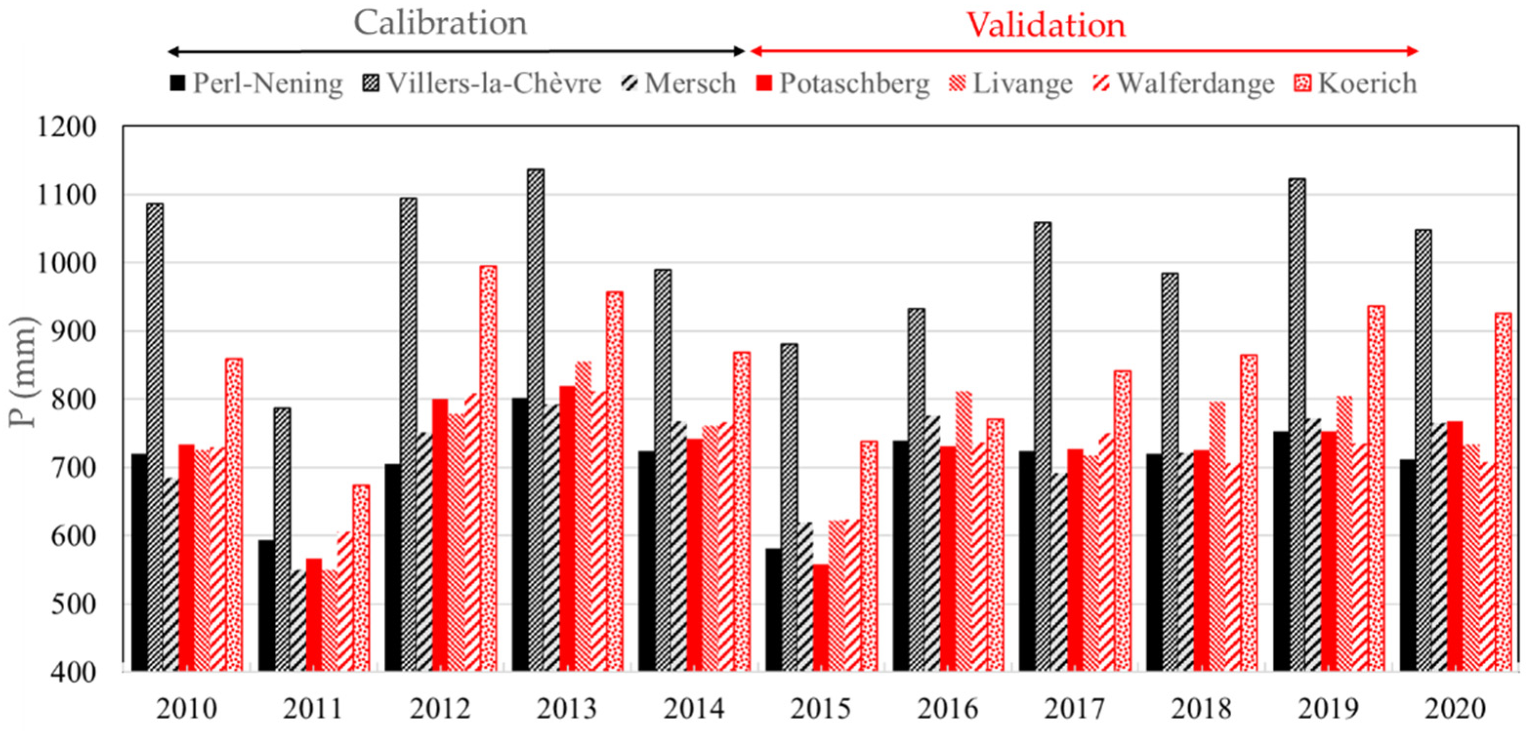
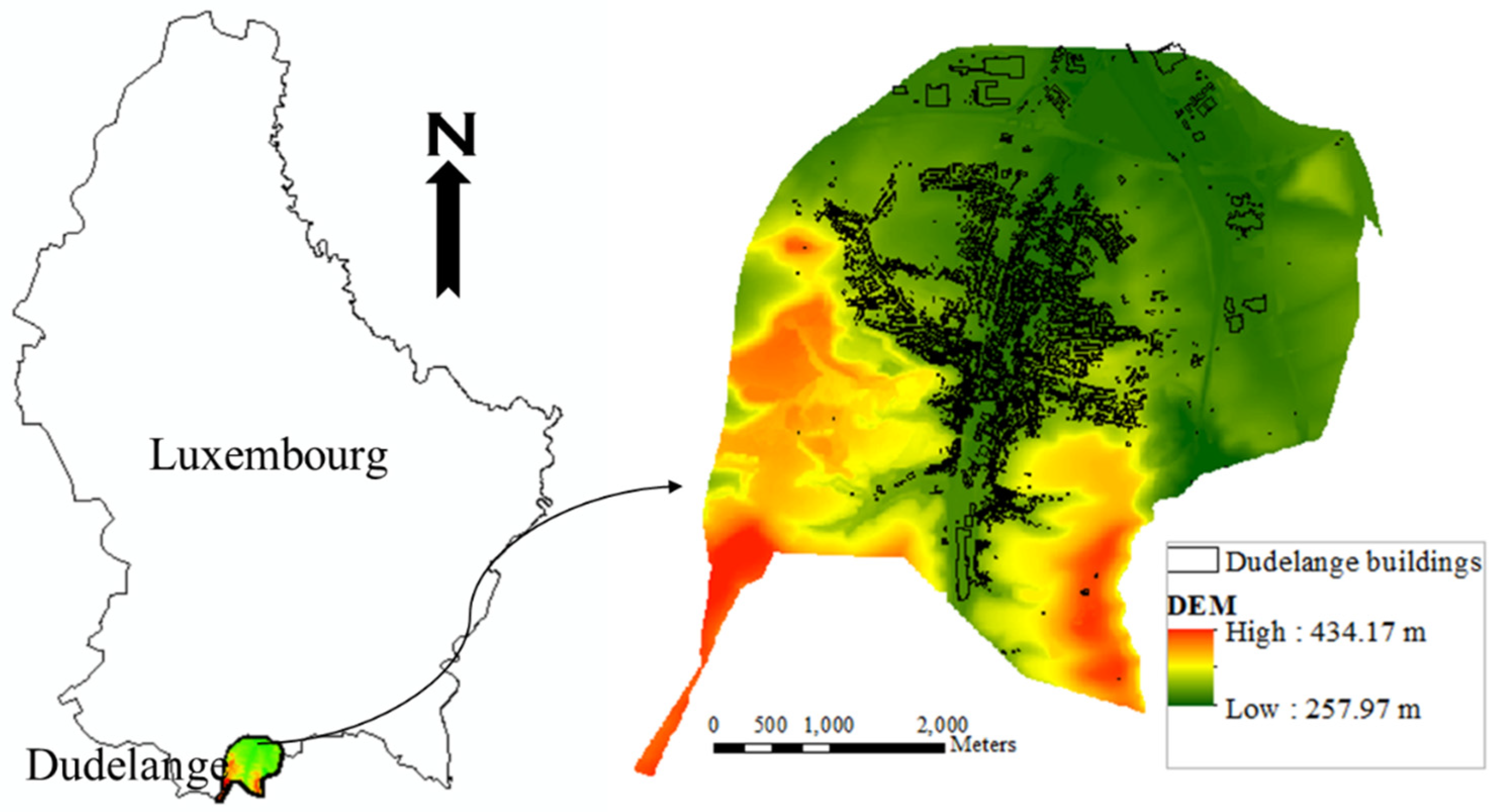
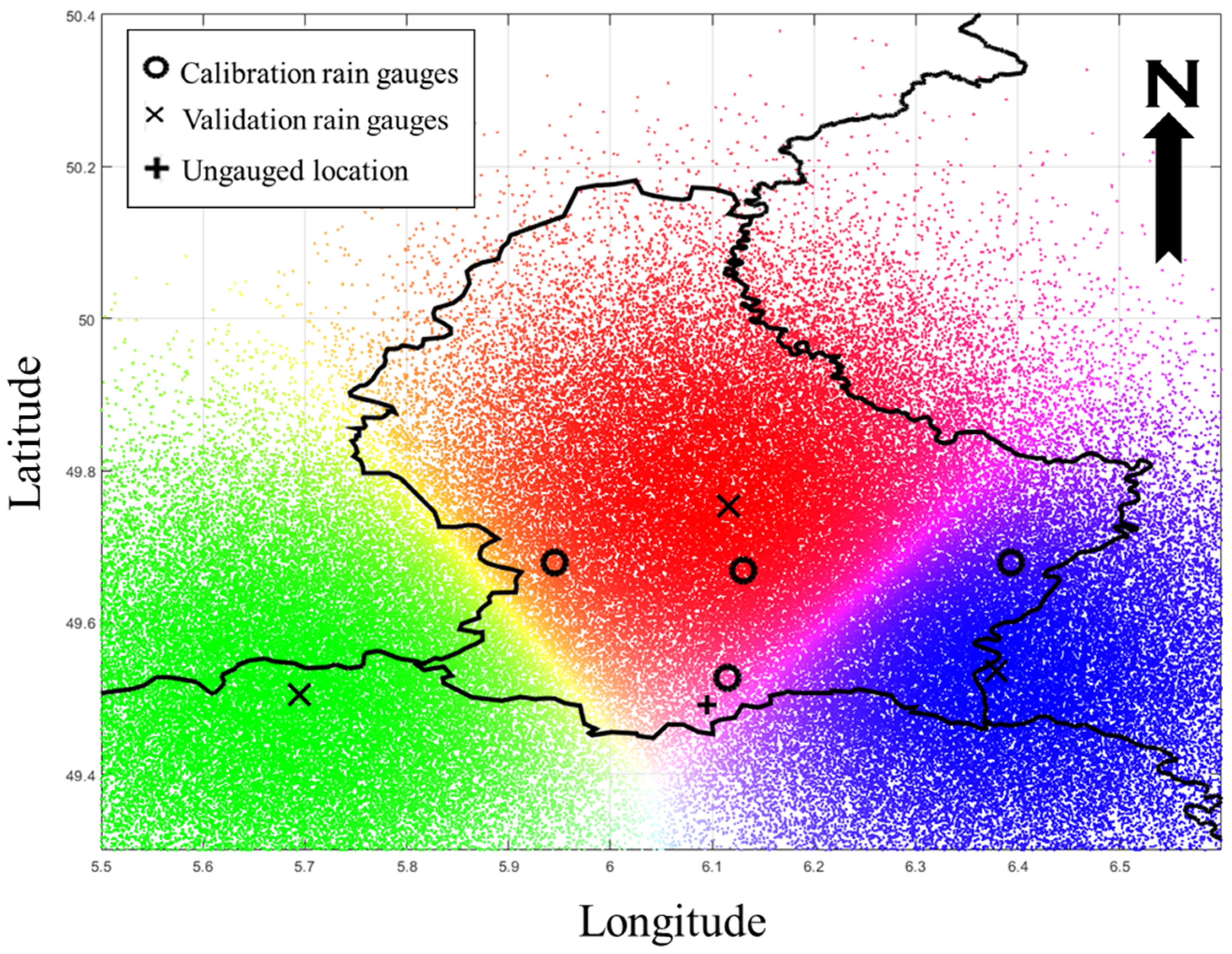
2.1. Study Area and Data

In order to simulate floods as well as develop the i-FCM methodology for rainfall data, the city of Dudelange, located in southern Luxembourg, was selected as a case study, due to a lack of local rainfall observations albeit its risk exposure to localized urban flashfloods. In this regard, seven rain gauge locations in Luxembourg (Mersch, Livange, Koerich, Potaschberg and Walferdange), Germany (Perl-Nening) and France (Villers-la-Chèvre) were chosen, as shown in Figure 1.
As shown in Figure 1, 3 locations were chosen for calibration stations, whereas 4 stations were considered as validation stations for the estimation of rainfall. The raw data are hourly rainfall data for a period of more than 11 years (January 2010–July 2021). Dudelange on the contrary the inverse Fuzzy C-Means (i-FCM) methodology will be applied for different time scales (daily and monthly). The annual precipitation in all observed stations is shown in Figure 2.
In order to simulate flood using LISFLOOD-FP, the digital elevation model (DEM) is needed. In this regard, a LiDAR-based Digital Elevation Model (DEM) of Dudelange with a spatial resolution of 50 × 50 cm and vertical accuracy of better than 20 cm, provided by Luxembourg Land Registry and Topography (ACT) was resampled to 3 × 3 m resolution in order to reduce computation time and consequently introduced to the flood model as an input (see Figure 3). To have a better understanding of the urbanization of the study area, the spatial distribution of buildings in the city is shown in Figure 3, as well.
As the above figure shows, the urban expansion occurred in the lower part of DEM. In other words, the city is located in a flood-prone area.

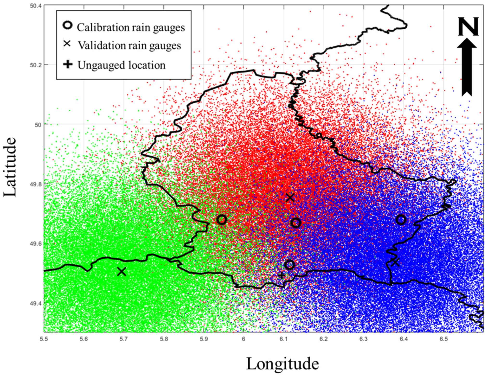
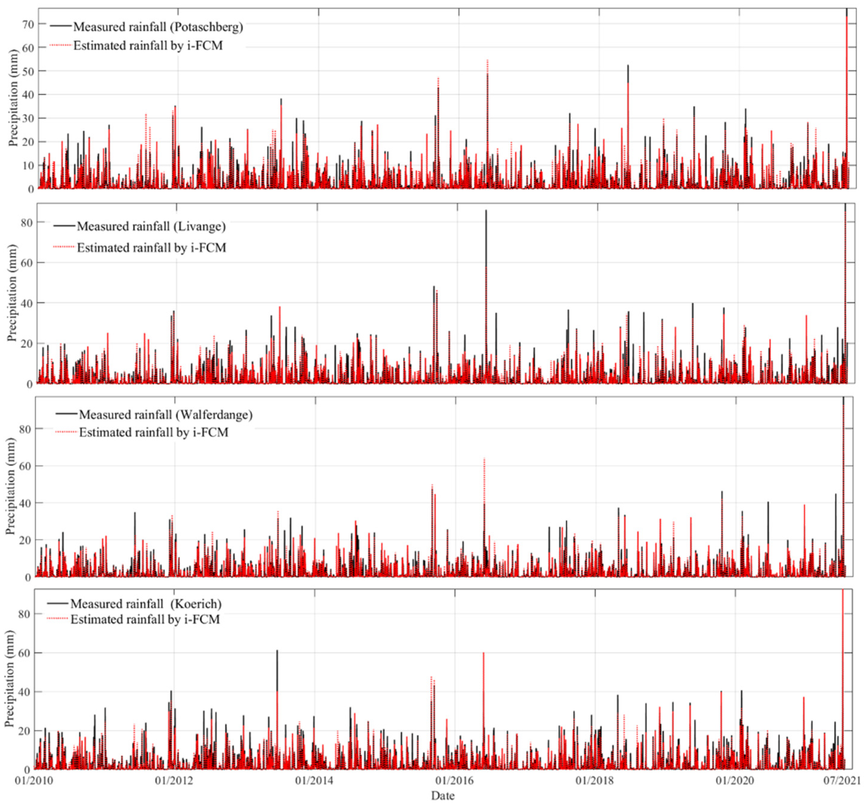
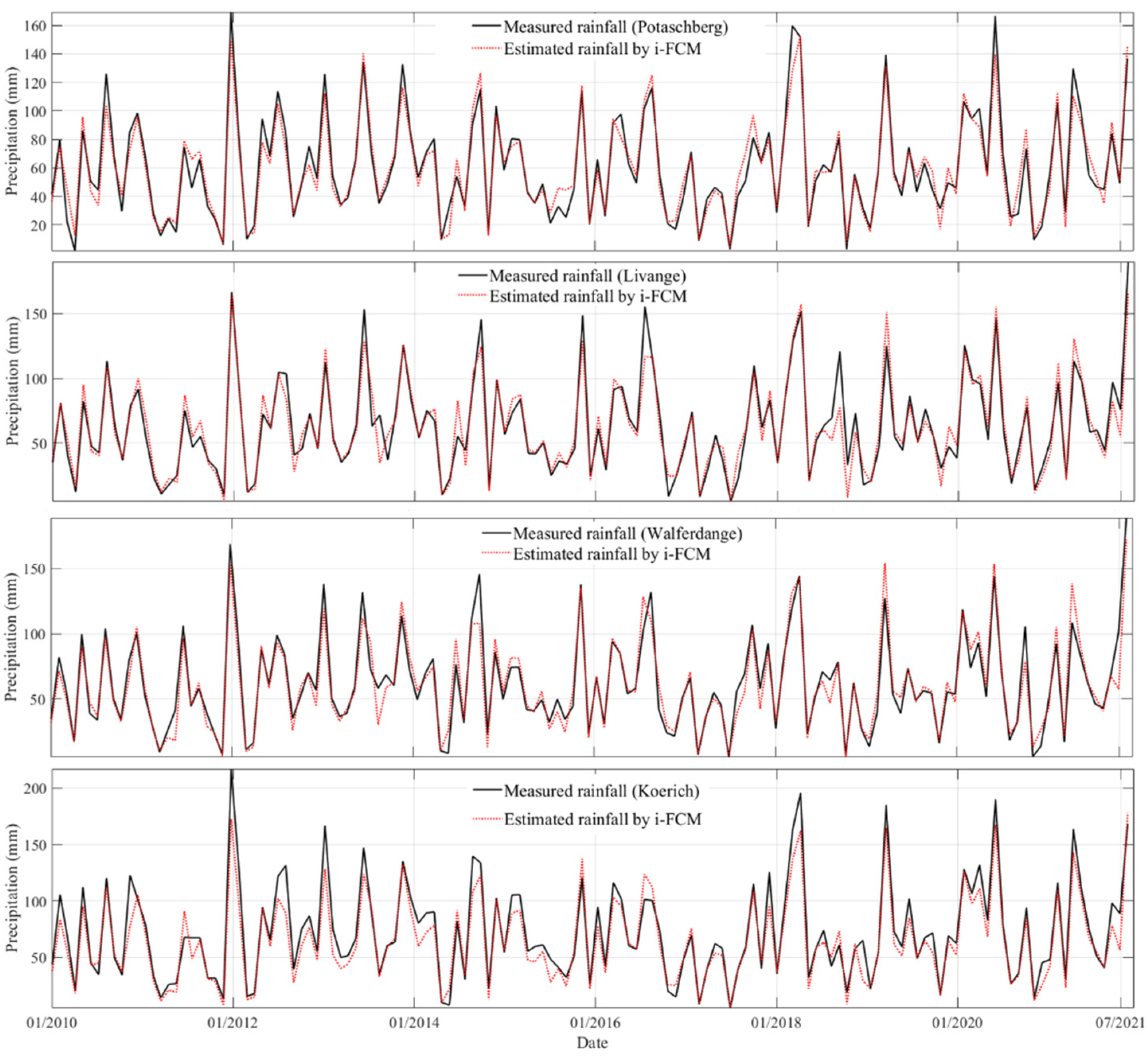
2.2. Estimation of Rainfall Data Using the i-FCM Clustering Method

Data clustering consists in categorizing the data set into specific groups, such that data sets with the same characteristics are incorporated into the same clusters and non-similar data sets belong to different clusters. Defining representative behavior of a multi-dimensional nonlinear system of large time-series data sets is the main objective of data clustering algorithms [8].
The FCM approach is known as an improvement and modification of the well-known K-means clustering [9,10]. In this approach, each data point belongs partly to all clusters, however, with different membership degrees that can vary between 0 and 1. The objective function in the FCM is minimizing the total intra-cluster variance, i.e., the summed square error function
  J m ( U ,   V ) = i = 1 c j = 1 n u i j m d 2 ( x j , v i )
within clusters   ( J m ) [11,12], where U = [uij]c×n is the fuzzy partition matrix of c clusters and n data, V = (v1, v2, ….., vi) are the centers of the clusters, uij is the partial membership degree of data xj in cluster i ( 0 u i j 1     &   i = 1 c u i j = 1   ,       j = 1 , 2 , , n ) , m is the weighting exponent on each fuzzy membership. Regarding [13] suggestion, the best choice for m is a value between 1.5–2.5 (which is equal to 2 in this study), xj = (x1, x2, ….., xn) is the dataset, vi is the initial value for a cluster center and d(xj, vi) is the Euclidean distance between the xj data and the cluster center of the i-th cluster vi, i.e., x j v i .
Equation (1) describes a non-linear optimization problem which can be solved by iterative minimization. The center of each cluster is calculated using the partial derivative of Equation (1) with respect to V, then the partial membership degree of the data will be updated in each iteration by differentiation of the above equation with respect to U:
u i j = ( k = 1 c ( d ( x j   ,     v i ) d ( x j   ,     v k ) ) 2 m 1 ) 1               ,   i = 1 , 2 , ,   c   ;         j = 1 , 2 , ,   c   ;    
The iteration process is stopped if the variance of intra-cluster in 5 iterations does not change more than the determined minimum improvement (in this study 10−8), i.e., a minimum improvement in the FCM objective function (convergence) does not occur in 5 iterations and/or the maximum number of iterations (1000 iterations in the present study) is exceeded.
As indicated above, in the normal FCM procedure clusters’ centers are determined in an iterative parameter estimation and consequently the degree of data membership [0, 1] of each data point will be calculated. Differently, in the present study, with i-FCM the center of each cluster (weather stations with measured rainfall data) is known a priori and does not change, while random data will be generated using a multivariate normal distribution with the following probability density function for x :
p ( x ; μ , σ X Y ) = 1 ( 2 π ) n / 2 ( σ X Y ) 0.5 e x p ( 1 2 ( x μ )   σ X Y 1 ( x μ ) )
where μ is center of the cluster (weather stations) with X, Y coordinates; σ X Y is the covariance matrix (= [1 1] × 2.5 × 10−2), n is number of data points around each cluster center, which is set equal to 50,000 points (see Figure 4).
Therefore, the whole FCM process was inverted. In FCM, the clustering is performed on data based on a predefined number of clusters for which the centers of the clusters need to be calculated. On the contrary, in this study, the centers of the clusters were determined first as the locations of the weather stations and the data will be generated based on these cluster centers: this is the reason to name this method the inverse FCM (i-FCM).

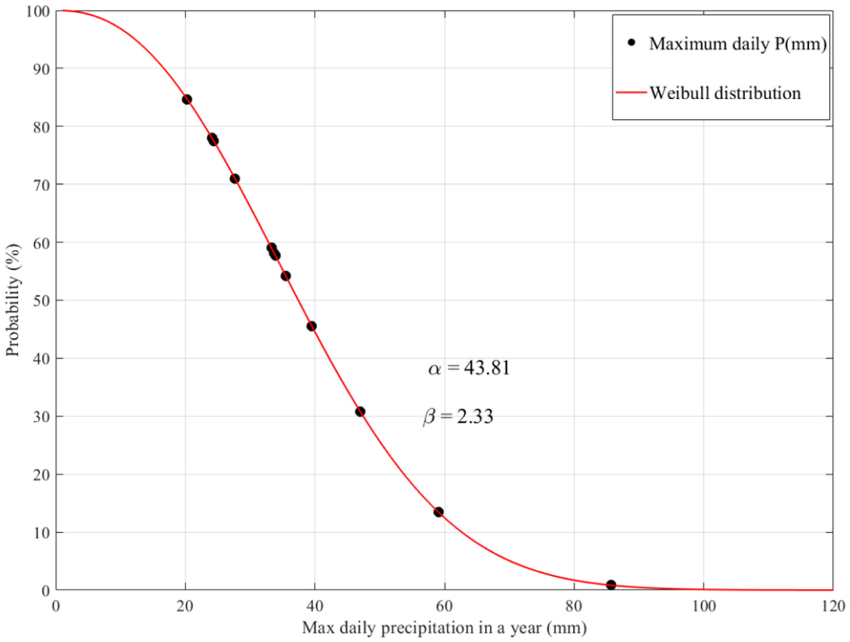
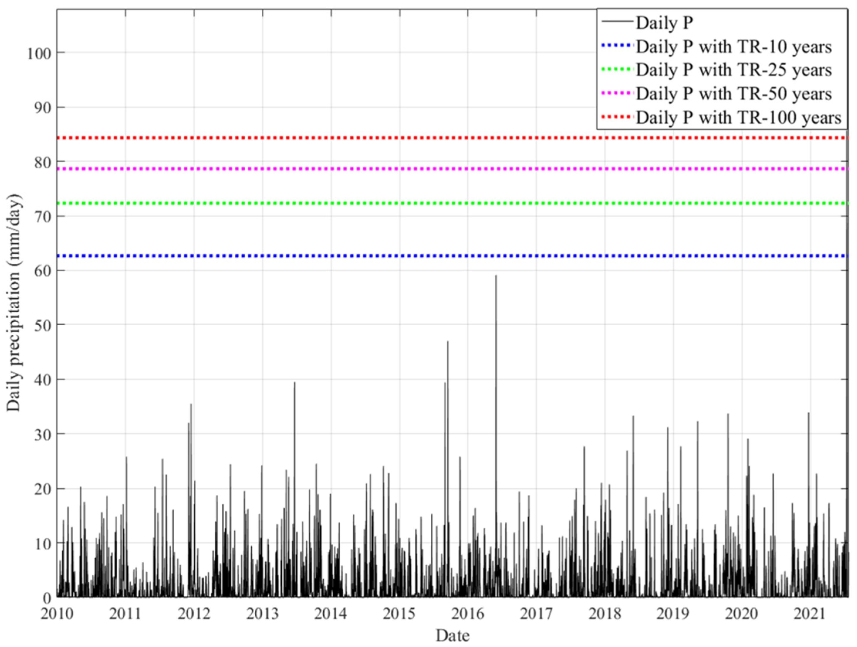
2.3. Return Period (Tr) Estimation for Maximum Daily Rainfall

Flooding happens after extreme rainfall events. The frequency analysis used to calculate maximum daily rainfall with different return periods of 10, 25, 50 and 100 years, can be used as input to the LISFLOOD-FP flood model. There have been a lot of discussions for quite some time in the hydrological literature on the appropriateness of the Weibull for calculating return periods [14,15,16,17]. For this reason, a two-parameter Weibull distribution [18] with the following probability density function (pdf) was used in the present study:
f ( x | α , β ) = β α ( x α ) β 1 e ( x / α ) β
where f ( x ) is pdf; α   and   β are shape and scale parameters, respectively, was fitted to the i-FCM estimated maximum daily rainfall of each year in Dudelange during the time period of January 2010 to July 2021, using nonlinear maximum likelihood estimation (MLE). The cumulative distribution function (F(x)) is
F ( x ) =   P ( X x i ) = 0 x f ( t ) d t
The magnitude of Tr is the given value for the inverse of the probability of occurrence P (XxTr) which is equal to 1 − F(xTr), i.e., Tr = [1 − P (XxTr)]−1.

2.4. Flood Hazard Maps Using LISFLOOD FP Model

The flood hazard maps based on rainfall events with 10, 25, 50 and 100 years were generated by widely and successfully applied LISFLOOD-FP flood model. This model is developed by the University of Bristol [19,20] which allows computation of water depth flows and 2-D water flow velocity in each cell of the raster grid across floodplains. It is based on a modified version of the momentum and continuity equations of full shallow water, neglecting only the convection force term, which can be assumed negligible [21]. In order to calculate a flood hazard value in each cell of the raster map, the LISFLOOD FP model requires spatial and temporal data as inputs. The spatial data are land elevation of each cell (extracted from the DEM), north–south and east–west boundary conditions of the study area and Manning’s roughness coefficient (n = 0.065). The temporal data are rainfall data for specific return periods in mm.hr−1. Once the inputs are introduced to the model, the water depth and flow velocity in each cell was computed and consequently, the flood hazard value will be calculated based on these two factors (Equations (6) and (7)) [22]
V c i , j = [ m a x ( V i 0.5 , j + V i + 0.5 , j ) ] 2 + [ m a x ( V i , j 0.5 + V i , j + 0.5 ) ] 2
H z i , j = D i , j ( V c i , j + 1.5 )
where V c i , j , D i , j and H z i , j are water velocity, water depth and flood hazard data in cell (i,j), respectively. The hazard rating classes shown in Table 1 is used to define a degree of hazard for people in flood events [21,22]

3. Results and Discussion

3.1. i-FCM Spatial Interpolation for Precipitation

In this study, the newly introduced i-FCM method was used as a spatial interpolation methodology to estimate rainfall data for an ungauged location (Figure 5). After calculating the membership degrees of all random data (n = 1.5 × 10⁴ around three rain gauge locations), these 3 degrees for each point were applied to estimate rainfall data in four validation rain gauges. For the statistical analysis of the results of the i-FCM method, R2 parameters were computed for estimated and measured daily and monthly rainfall (Figure 6). As Figure 7 and Figure 8 show, there is a good agreement between the i-FCM-simulated and measured data at the validation point location, with a high R2 (=0.94 to 0.98, 0.86 to 0.89) and a low RMSE (=9 to 14, 1.67 to 2 mm) for both monthly and daily time scales. Although the statistical parameters (R2 and RMSE) show that there is not a significant difference in the accuracy of the i-FCM method between the validation stations, the results in Potaschberg are slightly better which could be related to its greater spatial distance from the calibration station in France (Villers-la-Chèvre). There the annual rainfall shows that it is the most humid area among all calibration stations (See Figure 2). In other words, the distance from the latter calibration station has an inverse relationship with accuracy. All data-driven estimation methods are based on the idea that the random errors are drawn from a normal distribution [23] and the i-FCM model is no exception. Figure 9 illustrates that the posteriori computed errors of the rainfall estimation with this model follow indeed such a normal distribution.
The above results figures show that the i-FCM model can be applied as a spatial interpolation method to estimate rainfall in an ungauged location, such as Dudelange, as in the case presented here and using relevant membership degrees. The results for this ungauged location are shown in Figure 10 below.
The results reported here clearly indicate that the i-FCM methodology delivers very good and reliable estimated rainfall data for a local case study. The reason is due to the fact that this spatial interpolation method uses the advantages of fuzzy logic and clustering simultaneously. We believe that the method introduced here could be added to current interpolation methods, as summarized for example in [5].

3.2. Estimation of Maximum Daily Rainfall Return Periods Using Two-Parameter Weibull Distribution

The return periods of the Dudelange maximum daily rainfall are calculated by the two-parameter Weibull distribution over the observation time interval (January 2010 to July 2021). maximum daily rainfall events in a year for different probabilities p are computed in this method from the corresponding quantiles of the fitted Weibull distribution. The results are shown by the smooth lines in Figure 11. The parameters of the Weibull distribution were estimated within the 95% confidence interval, i.e., α   and   β are equal to 43.81 and 2.33 within the 95% confidence interval of (33.83, 56.72) and (1.56, 3.47), respectively.
Figure 12 shows the corresponding rainfall values for return periods of 10, 25, 50 and 100 years obtained with frequency analysis method using 2-parameter ( α   and   β ) Weibull distribution.

3.3. Generating Flood Hazards Maps Using LISFLOOD FP Model

In order to illustrate the value of the proposed interpolation method for ungauged locations in relation to a downstream application, the interoperated rainfall for different return periods was introduced to a 2-D flood model as one of the inputs, with the assumption of antecedent rainfall of 0.04 mm/hr (equal to 1 mm/day) on the area for 6 h to eliminate the effects initial losses in rainfall-runoff process. Therefore, the whole estimated rainfall for a specific return period will be considered as excessive precipitation by LISFLOOD FP model. By adding other inputs and parameters, namely, the digital elevation model (DEM) and Manning’s roughness coefficient (n) of 0.065 the model was run and flood hazards maps were generated (Figure 13). In order to see the effects of rainfall intensity on flood hazards, the involved area (ha) to moderate, significant and extreme hazards are listed in Table 2. As can be seen, the hazardous flooded area with the 100-years return period rainfall event is 33% more than 10-years ones, this value is 12% and 5% larger in comparison to the 25 and 50-years return periods, respectively. In addition, the urban part of the city where buildings are located is the most vulnerable area for flood events which shows that integrated flood management is needed in view of better flood protection measures.
In this study, an inverse FCM (i-FCM) method was introduced for spatial interpolation of rainfall data at an ungauged location–in our case the city of Dudelange, Luxembourg. The reason to name this method the inverse FCM is that the centers of the clusters are a priori set to be the locations of the weather stations and the data are then generated based on these cluster centers.
In the case presented here, the daily and monthly rainfall-data series were measured at seven rain gauge locations. Three of the measured time series were used directly as inputs to the i-FCM model to calculate membership degrees for the generated data and then the data of the four remaining rain gauges were considered for validation. The results of the proposed i-FCM model illustrate that the combination of fuzzy logic and clustering appears to be a reliable tool for spatial interpolation at different time scales. Such interpolated rainfall data can now be generated for any location using i-FCM, which could hold promise for local impact studies of evapotranspiration, droughts and floods, as well as for a variety of water management planning projects. This interpolation can be added as a methodology of spatial interpolation of hydrological data which is indicated in the introduction part such as [5,6]. The main goal of present study is coupling a hydraulics flood model with statistical (calculating return period) and data driven machine learning (spatial interpolation with i-FCM) method to generate flood hazard maps in ungauged station. The combination of these models and algorithms has led to even an increased accuracy in the modeling of floods and will thus help water authorities to better plan for flood management policies.

4. Conclusions

This application of flood models for determining the flood hazard is one of the major titles in water resources planning and management. Obviously, in the process of studying extreme hydrological events like flooding in an urban area, the accurate estimation of rainfall data in any ungauged location is very important. A machine learning (ML) clustering method as an efficient, fast, accurate yet simple tool was introduced in this study, named i-FCM spatial interpolation. A two-dimensional numerical model is a very useful tool to show the flood hazard maps after an intensive rainfall event. The combination of the proposed ML method and a hydrodynamic model is a practical scientific-based approach to increase the accuracy in the modeling of flood events. In this study, a LISFLOOD FP flood model was applied for generating hazard maps in an urban floodplain, Dudelange, southern Luxembourg. More specifically, the rainfall data were estimated by i-FCM method for ungauged location firstly. The statistical analysis of the validation stations shows that the i-FCM spatial interpolation method works appropriately. In the next step, a frequency analysis statistical method was applied to calculate the probability of occurrence (or different return periods) of maximum daily rainfall events using the two-parameter Weibull distribution. Finally, interpolated rainfall data and digital elevation model (DEM) are used as input to the flood model to get corresponding flood hazard spatial distribution.
In conclusion, the innovative i-FCM method coupled with a statistical method and a flood model proposed here reveals itself to be a helpful tool for developing efficient flood hazard estimation at the very local scale, in particular, where there is a lack of data (ungauged location) with the aim to help provide better flood mitigation.

Author Contributions

Conceptualization, M.Z.; methodology, M.Z.; software, M.Z. and G.J.-P.S.; validation, M.Z., G.J.-P.S. and F.N.T.; formal analysis, M.Z.; investigation, M.Z.; data curation, M.Z. and R.M.; writing—original draft preparation, M.Z.; writing—review and editing, G.J.-P.S. and F.N.T.; visualization, M.Z. and R.M.; supervision, G.J.-P.S.; project administration, G.J.-P.S. and F.N.T.; funding acquisition, M.Z., G.J.-P.S. and F.N.T. All authors have read and agreed to the published version of the manuscript.

Funding

This research was funded by the Luxembourg National Research Fund (FNR) in the framework of an industrial fellowship with Ref. No. 14111453.

Data Availability Statement

All precipitation data of Luxembourg are available for download from the webpage (https://www.agrimeteo.lu (accessed on 15 September 2021)) of agro-meteorological weather service department of Administration des Services Techniques de l’Agriculture (ASTA), Luxembourg. The precipitation data in Germany and France was provided by Deutscher Wetterdienst (DWD) (German Weather Service) and DREAL Grand Est-Service de prévention des risques naturels et hydrauliques, respectively.

Conflicts of Interest

The authors declare no conflict of interest.

References

  1. IPCC. Summary for policymakers. In Climate Change 2007: The Physical Science Basis. Contribution of Working Group I to the Fourth Assessment Report of the Intergovernmental Panel on Climate Change; Solomon, S., Qin, D., Manning, M., Chen, Z., Marquis, M., Averyt, K.B., Tignor, M., Miller, H.L., Eds.; Cambridge University Press: Cambridge, UK, 2007. [Google Scholar]
  2. Zare, M.; Koch, M. An Analysis of MLR and NLP for Use in River Flood Routing and Comparison with the Muskingum Method. In Proceedings of the 11th International Conference on Hydroscience & Engineering (ICHE), Hamburg, Germany, 29 September–2 October 2014; pp. 505–513. [Google Scholar]
  3. Courty, L.G.; Rico-Ramirez, M.Á.; Pedrozo-Acuña, A. The Significance of the Spatial Variability of Rainfall on the Numerical Simulation of Urban Floods. Water 2008, 10, 207. [Google Scholar] [CrossRef] [Green Version]
  4. Crochet, P.; Jóhannesson, T.; Jónsson, T.; Sigurðsson, O.; Björnsson, H.; Pálsson, F.; Barstad, I. Estimating the Spatial Distribution of Precipitation in Iceland Using a Linear Model of Orographic Precipitation. J. Hydrometeorol. 2007, 8, 1285–1306. [Google Scholar] [CrossRef]
  5. Hu, Q.; Li, Z.; Wang, L.; Huang, Y.; Wang, Y.; Li, L. Rainfall Spatial Estimations: A Review from Spatial Interpolation to Multi-Source Data Merging. Water 2019, 11, 579. [Google Scholar] [CrossRef] [Green Version]
  6. Drogue, G.; Ben Khediri, W. Catchment model regionalization approach based on spatial proximity: Does a neighbor catchment-based rainfall input strengthen the method? J. Hydrol. Reg. Stud. 2016, 8, 26–42. [Google Scholar] [CrossRef] [Green Version]
  7. Zadeh, L.A.; Aliev, R.A. Fuzzy Logic Theory and Applications, Part I and Part II; World Scientific Publishing Co.: Singapore, 2018. [Google Scholar]
  8. Çakıt, E.; Karwowski, W. Fuzzy Inference Modeling with the Help of Fuzzy Clustering for Predicting the Occurrence of Adverse Events in an Active Theater of War. Appl. Artif. Intell. 2015, 29, 945–961. [Google Scholar] [CrossRef]
  9. Bezdek, J.C.; Ehrlich, R.; Full, W. FCM: The fuzzy c-means clustering algorithm. Comput. Geosci. 1984, 10, 191–203. [Google Scholar] [CrossRef]
  10. Jafari, M.M.; Ojaghlou, H.; Zare, M.; Schumann, G.J. Application of a Novel Hybrid Wavelet-ANFIS/Fuzzy C-Means Clustering Model to Predict Groundwater Fluctuations. Atmosphere 2021, 12, 9. [Google Scholar] [CrossRef]
  11. Ayvaz, M.T.; Karahan, H.; Aral, M.M. Aquifer parameter and zone structure estimation using kernel-based fuzzy c-means clustering and genetic algorithm. J. Hydrol. 2007, 343, 240–253. [Google Scholar] [CrossRef]
  12. Zare, M.; Koch, M. Groundwater level fluctuations simulation and prediction by ANFIS- and hybrid Wavelet-ANFIS/Fuzzy C-Means (FCM) clustering models: Application to the Miandarband plain. J. Hydro-Environ. Res. 2018, 18, 63–76. [Google Scholar] [CrossRef]
  13. Pal, N.R.; Bezdek, J.C. On cluster validity for the fuzzy c-means model. IEEE Trans. Fuzzy Syst. 1995, 3, 370–379. [Google Scholar] [CrossRef]
  14. Hirsch, R.M. Probability plotting position formulas for flood records with historical information. J. Hydrol. 1987, 96, 185–199. [Google Scholar] [CrossRef]
  15. Chow, V.T.; Maidment, D.R.; Mays, L.W. Applied Hydrology; McGraw-Hill: New York, NY, USA, 1988. [Google Scholar]
  16. Cunnane, C. Unbiased plotting positions—A review. J. Hydrol. 1978, 37, 205–222. [Google Scholar] [CrossRef]
  17. Zare, M.; Koch, M. Hybrid signal processing/machine learning and PSO optimization model for conjunctive management of surface–groundwater resources. Neural Comput. Appl. 2021, 33, 13. [Google Scholar] [CrossRef]
  18. Pook, L.P. Approximation of Two Parameter Weibull Distribution by Rayleigh Distributions for Fatigue Testing; National Engineering Laboratory Report 694; East Kilbride: Glasgow, UK, 1984. [Google Scholar]
  19. Neal, J.; Schumann, G.; Bates, P. A subgrid channel model for simulating river hydraulics and floodplain inundation over large and data sparse areas. Water Resour. Res. 2012, 48, W11506. [Google Scholar] [CrossRef]
  20. Hawker, L.; Neal, J.; Tellman, B.; Liang, J.; Schumann, G.; Doyle, C.; Sullivan, J.A.; Savage, J.; Tshimanga, R. Comparing earth observation and inundation models to map flood hazards. Environ. Res. Lett. 2020, 15, 12. [Google Scholar] [CrossRef]
  21. Bates, P.; Trigg, M.; Neal, J.; Dabrowa, A. LISFLOOD-FP User Manual, Code Release 5.9.6; University of Bristol: Bristol, UK, 2013. [Google Scholar]
  22. Ramsbottom, D.; Floyd, P.; Penning-Rowsell, E. Flood Risks to People Phase 1, R&D Technical Report FD2317; DEFRA: London, UK, 2003.
  23. Beck, J.V.; Arnold, K.J. Parameter Estimation in Engineering and Science; John Wiley & Sons: Hoboken, NJ, USA, 1977; p. 522. [Google Scholar]
Figure 1. This is a figure. Schemes follow the same formatting.
Atmosphere 12 01336 g001
Figure 2. Annual rainfall of calibration and validation stations.
Atmosphere 12 01336 g002
Figure 3. Digital elevation model (DEM) and built-up areas of Dudelange, southern Luxembourg.
Atmosphere 12 01336 g003
Figure 4. Generating random data using a multivariate normal distribution (red, blue and green points are random data around cluster centers/calibration stations).
Atmosphere 12 01336 g004
Figure 5. Fuzzy C-means (FCM) clustering on generated data (i-FCM method).
Atmosphere 12 01336 g005
Figure 6. Regression plot of i-FCM model, estimated over observed P(mm); (Left) panel: monthly and (Right) panel: daily rainfall data.
Atmosphere 12 01336 g006
Figure 7. Measured and estimated daily rainfall data in validation stations.
Atmosphere 12 01336 g007
Figure 8. Measured and estimated monthly rainfall data in validation stations.
Atmosphere 12 01336 g008
Figure 9. Normal distribution of errors in validation stations; (Left) panel: daily rainfall data; (Right) panel: Monthly rainfall data.
Atmosphere 12 01336 g009
Figure 10. Estimated rainfall for Dudelange (ungauged). (Left) panel: daily, (Right) panel: monthly rainfall data.
Atmosphere 12 01336 g010
Figure 11. Two-parameter Weibull distribution (red line) for maximum daily rainfall.
Atmosphere 12 01336 g011
Figure 12. Return periods of maximum daily rainfall in Dudelange.
Atmosphere 12 01336 g012
Figure 13. Flood hazard maps based on different return period rainfall events.
Atmosphere 12 01336 g013
Table 1. Flood hazard classes [22].
Flood Hazard RatingDegree of Flood HazardDescription
0 No hazard-
<0.75LowCaution; Very low danger
0.75–1.25ModerateDanger for some
1.25–2.5SignificantDanger for most
>2.5ExtremeDanger for all
Table 2. The allocated area (ha) to the different classes of flood hazard (moderate to extreme).
Hazard RatingTr-10Tr-25Tr-50Tr-100
0.75–1.2530.2032.9135.5433.16
1.25–2.523.9929.8029.2734.17
>2.519.4424.4227.9030.36
Sum (ha)73.6387.1392.7197.69
Publisher’s Note: MDPI stays neutral with regard to jurisdictional claims in published maps and institutional affiliations.

