
Vehicle Emissions and Air Quality: The Early Years (1940s–1950s)


1
Desert Research Institute, Reno, NV 89512, USA
2
Chevron Products Company, San Ramon, CA 94583, USA
*
Author to whom correspondence should be addressed.
†
Retired.
Atmosphere 2021, 12(10), 1354; https://0-doi-org.brum.beds.ac.uk/10.3390/atmos12101354
Submission received: 13 September 2021
/
Revised: 11 October 2021
/
Accepted: 13 October 2021
/
Published: 16 October 2021
(This article belongs to the Special Issue Air Quality Impacts of Vehicle Emissions)
Abstract
:During the 1940s, an unusual form of air pollution was experienced in the Los Angeles (LA) area of Southern California. Referred to as LA smog, this pollution differed from previously known air pollution with respect to its temporal patterns (daytime formation and nighttime dissipation), eye irritation, high oxidant levels, and plant damage. Early laboratory and field experimentation discovered the photochemical origins of LA smog. Though mechanistic understanding was incomplete, it was determined that hydrocarbon (HC) compounds in the atmosphere participate in smog formation, enabling build-up of higher ozone concentrations than would otherwise occur. It being a significant source, there was great interest in characterizing and controlling HC emissions from motor vehicles. Considerable work was done in the 1940s and 1950s to understand how emissions varied with vehicle operating conditions and deterioration of engine components. During this time, procedures were developed (and improved) to sample and quantify vehicle emissions. Besides exhaust, HC emissions from crankcase blowby, carburetor evaporation, and fuel tank losses were measured and characterized. Initial versions of both catalytic and non-catalytic exhaust after-treatment systems were developed. The knowledge gained from this pre-1960 work laid the foundation for many advancements that reduced vehicle emissions and improved air quality during subsequent decades.

1. Introduction
Coinciding with the rapid growth of personal automobile usage following the end of World War II, an unusual form of air pollution began to be noticed in the Los Angeles (LA) area of southern California. The term “smog,” being a combination of smoke and fog, was used when referring to this pollution, though, as explained later, this term was not accurate. Throughout the latter half of the 1940s and all of the 1950s, considerable efforts were undertaken to characterize this unique form of LA smog and to understand its causes and effects. Early on, it was suspected that vehicle emissions were associated with the problem, though a full understanding of this did not develop until much later.
Extensive research efforts involving the fumigation of plants, smog chamber experiments, and detailed chemical analysis of ambient air all led to an improved understanding of smog formation and the role played by motor vehicles. These early decades saw many R&D (research and development) discoveries, successes, and failures. Much of this early history has faded from memory, but it should be recalled, as it forms the foundation upon which today’s clean, efficient, and high-performance vehicles are based.
While similar vehicle pollution control programs have been implemented in many countries, this paper focuses exclusively on the U.S. situation. The earliest work regarding smog, vehicle emissions, and control measures occurred in California, which has remained a center of activity in these areas for the past 75 years. With the establishment of the U.S. Environmental Protection Agency (EPA) in 1970—and earlier activities leading up to this event—the federal government also became (and continues to be) a major player in this arena.
We also limit our attention to light-duty vehicles, as these are the most common application of gasoline engines and are- most familiar to the public. It is recognized, however, that similar technology developments have occurred with other vehicle applications. Furthermore, our focus is on pollutant emissions associated with smog or other health-concerning effects. Thus, carbon dioxide (CO2) emissions, which were dealt with at the same time, are not considered here. It should also be noted that the information sources used in this review rely heavily upon published literature, which tends to present a “cleaner” and more definitive view of certain events than existed at the time they occurred.
2. Early Concerns about Air Pollution in Los Angeles
Following the end of World War II, the U.S. experienced a period of dramatic expansion of population, urbanization, and prosperity—driven in part by increased mobility afforded by the motor vehicle. No place is a better example of this than Southern California, particularly the greater LA area. Between 1940 and 1950, the population of LA County increased by about 50%, from 2.78 million to 4.15 million [1]. During this period, the number of automobiles in California increased from 2.5 million to 4.0 million, with approximately one-half of these totals being within the LA area [2].
2.1. Early History of Air Pollution
The term “smog” is a contraction of the words smoke and fog. Although the first scientific use of this term is often attributed to Dr. Henry Antoine Des Voeux in a 1905 paper, the word itself was apparently used some 25 years earlier [3]. As originally used, smog referred to air pollution resulting primarily from coal combustion emissions, under atmospheric conditions that prevented dispersion of the pollutants. The main chemical constituents in smog were soot (particulate matter) and sulfur oxides. This type of smog was problematic in many industrialized cities during the first half of the 20th Century—most famously, London, which suffered a catastrophic smog event in December 1952, during which 4000 fatalities occurred. In the U.S., the most noteworthy (and deadly) smog episode occurred in October of 1948, in the small town of Donora, Pennsylvania. A classic photo of this event is shown in Figure 1.
2.2. Los Angeles Smog
Although the same word, “smog,” is used to describe the type of air pollution for which Los Angeles is known, the formation, composition, and effects of modern, urban smog are quite different from previous air pollution episodes that occurred in London, New York, and many other cities prior to the 1940s. Unlike the earlier coal-derived smog, LA smog was observed primarily during summer months, but only during daytime hours. LA smog was also characterized by severe eye irritation (including lachrymatory effects (formation of tears)), its sharp odor (which was compared to that of bleach), and its deleterious effects on rubber materials. A useful comparison of London and Los Angeles smog, published in 1962, is summarized in Table 1 [4].
In addition to its large population and numerous sources of pollutant emissions, the greater LA area, often referred to as the South Coast Air Basin (SoCAB), has meteorological and geological features that are conducive to the formation and persistence of photochemical smog. To the north and east, the SoCAB is bounded by a semicircular ring of mountains, which help confine air pollution within the basin. During much of the year, a gentle sea breeze moves pollutants inland during the daytime, with a reversal of wind direction at night. This back-and-forth movement of air masses, along with frequent temperature inversion conditions that keep pollutants close to ground level, enable multi-day smog events in the SoCAB.
The first serious smog episode recognized in LA occurred on 26 July 1943, during World War II. As reported in the Los Angeles Times, “A pall of smoke and fumes descended on downtown, cutting visibility to three blocks. Striking in the middle of a heat wave, the ‘gas attack’ was nearly unbearable, gripping workers and residents with an eye-stinging, throat-scraping sensation. It also left them with the realization that something had gone terribly wrong in their city, prized for its sunny climate” [5]. Initial statements from city officials blamed emissions of butadiene from a synthetic rubber plant located near the center of Los Angeles and operated by the Southern California Gas Company. Due to public pressure, this plant was temporarily shut down, but the recurrence of similar smog episodes demonstrated that the plant was not the chief cause of the regional air quality problem.
2.3. Initial Governmental Action
In October 1943, just three months after the initial severe smog episode, the LA County Board of Supervisors appointed a Smoke and Fumes Commission to study the worsening air pollution problem. Following recommendations of this Commission, the County established the office of Director of Air Pollution Control in 1945. This office was granted the authority to enforce air pollution ordinances of the County—mostly dealing with excessive smoke issues.
Around the same time, the LA County Board of Supervisors approved draft legislation allowing California counties to establish unified air pollution control districts. Following passage of this Air Pollution Control Act by the California Legislature, the LA County Air Pollution Control District (LACAPCD) was established in October 1947. Because air pollution in the LA area was originally assumed to be similar to that in other locations, initial ordinances enacted by the LACAPCD focused on control of smoke and sulfur oxide emissions. For a more detailed account of the early development of air pollution legislation and regulations, the reader is referred to the literature [6,7].
2.4. Plant Damage from Smog
Air pollution-related injury to leafy agricultural crops in the LA area was first noted in 1944 [8]. While initially thought to result from exposure to sulfur dioxide (SO2), more extensive research indicated that the type of damage observed across a wide range of herbaceous plants was not consistent with that produced by SO2 alone, and some other harmful gaseous species must be involved. The crops experiencing the greatest economic loss due to air pollution damage included alfalfa, spinach, parsley, celery, sugar beets, and lettuce. It was noted that these problems were so serious as to cause some farming and nursery operations to relocate out of the SoCAB [8].
In the late 1940s and early 1950s, the LACAPCD, in collaboration with the California Institute of Technology (Caltech), undertook an extensive research program to determine what air pollutant species were responsible for this plant damage and to define safe concentrations of these species [9,10]. Much of the experimental work was conducted in the Earhart Plant Research Laboratory at Caltech in Pasadena, California. This newly built facility, also called the Phytotron, was a state-of-the-art laboratory that enabled plants to be grown under controlled conditions of temperature, lighting, humidity, and atmospheric composition [11,12]. The Earhart Plant Research Laboratory was operated under the leadership of Dr. Frits Went, an early researcher in the field of atmospheric chemistry, shown in Figure 2.
During this LACAPCD/Caltech program, numerous fumigation experiments were conducted in which many types of plants were exposed to individual chemical species (and combinations of species) at various concentrations. It was shown that plant damage during smog events in Pasadena could be eliminated if the ambient air was first purified by passing it through activated carbon filters. Fumigation of plants with ppm levels of many individual compounds (hydrocarbons, alcohols, aldehydes, ketones, ozone, and sulfur-containing compounds) failed to reproduce the plant damage observed during exposure to polluted ambient air. However, fumigation with the combination of ozone and hydrocarbons produced typical smog damage. This damage was most severe when using unsaturated hydrocarbons—also called alkenes or olefins. The researchers concluded that the observed plant damage was likely caused by organic peroxide compounds, which are formed by an ozonization process, in which ozone chemically reacts with olefins.
It was also demonstrated that the same type of plant damage occurred during fumigation experiments in which olefins (and gasoline vapors) were combined with nitrogen dioxide (NO2) and exposed to sunlight. Even though ozone itself was not added to these fumigation mixtures, it was likely produced during the photochemical process, thereby leading to the formation of the same damaging organic peroxides as described above. The researchers also noted that in many of these plant-damaging fumigation experiments, the same type of lachrymatory effects was observed as during ambient smog episodes.
Besides the eye irritation and rubber cracking effects of LA smog, its adverse economic impact on agricultural crops in Southern California was a strong motivator to understand the origins of this air pollution and to develop effective mitigation strategies. From this work, rudimentary understanding emerged regarding the chemical constituents and atmospheric conditions that were most conducive to smog formation.
By the end of the 1940s, it was beginning to be recognized that LA smog likely resulted from photochemical oxidation processes involving hydrocarbons and oxides of nitrogen (NOx), and ozone formation played an important role in these processes. It was further recognized that the sources of hydrocarbons were manifold, but chief among them were emissions associated with industry, municipalities, and the production, distribution, and use of gasoline. Emissions from motor vehicles were also recognized as contributing to these hydrocarbons, though this contribution was not believed to be very large.
3. Improved Understanding of Air Pollution
By the beginning of the 1950s, the phenomena of summer (photochemical) smog episodes were recognized as a serious and unique problem in the LA area. While some characteristics of this smog were well known—such as its odor, eye irritation, haze properties, plant damage, and rubber damage—there was very little fundamental understanding of how it formed and dissipated each day. It was believed that gaseous emissions of both hydrocarbons and oxides of nitrogen (NOx) were involved, along with photolytic action of sunlight, but the detailed chemical processes by which these primary pollutants reacted to produce secondary smog were not known.
Throughout the decade of the 1950s, great progress was made in characterizing smog and its precursor emissions and in understanding the chemistry of smog formation. This knowledge led to better-informed ideas about how to reduce the severity of smog episodes. Some of these ideas were acted upon by governmental regulatory bodies, which were formed to address the growing public problem of air pollution—primarily in California, but also beginning to occur in other locations.
3.1. Characterization of Air Pollution and Its Effects
It is perhaps a fortunate coincidence that Caltech is located in Pasadena, California. This location is downwind of Los Angeles and often experienced some of the most severe effects of smog episodes. By being located in the heart of the problem area, several Caltech researchers were led to assume early roles in understanding and mitigating LA smog. Most noteworthy among these scientific pioneers was Arie Jan Haagen-Smit (1900–1977; see Figure 3). In the 1950s, Haagen-Smit was already a well-known organic-analytical chemist who had established a successful research career focused on studying the chemistry of natural products. As part of this work, he had developed numerous sampling and analysis techniques to characterize trace levels of chemical species responsible for plants’ unique odors and flavors. This background and expertise proved to be ideal for the study of air pollution [13].
Smog formation in the LA area is an episodic phenomenon, with the spatial and temporal patterns varying somewhat from case-to-case, as well as from the severity and duration of each episode. Nevertheless, in 1950, Haagen-Smit characterized the most common meteorological conditions that occurred during typical smog events and described the usual spatial and temporal distributions of the smog air masses [14]. He also provided rough estimates of the number of pollutants involved in these episodes. For example, an air reservoir of 25 by 25 miles and 1000 feet deep (which Haagen-Smit used to approximate the volume of smog-polluted air in a typical episode) has a mass of about 650 million tons. Thus, a pollutant species that is uniformly present at a concentration of 1 ppm represents 650 tons of that pollutant. In comparison, only 80 tons of the organic aldehyde species, acrolein, dispersed in this air mass would be of sufficient concentration to cause eye irritation, and 400 tons of formaldehyde would cause tearing of the eyes.
Haagen-Smit pointed out that these quantities of pollutants were entirely possible within the LA area. He estimated that motor vehicles in LA used approximately 12,000 tons of gasoline each day. Assuming 99% combustion completion (which is surely overstated for that era) means that 120 tons per day of unburned (or partially burned) gasoline would be emitted from the vehicle fleet. Other large hydrocarbon sources included refineries, industries using volatile solvents, and the numerous private garbage incinerators that were still in existence at that time. In an early assessment of emission sources in Los Angeles County, the LACAPCD estimated total hydrocarbon emissions in 1951 to be 2180 tons/day, with gasoline vehicles being responsible for about 40% of this total [15]. Total NOx emissions were estimated at 255 tons/day, with gasoline vehicles being responsible for about 50% of the total.
Haagen-Smit and others conducted extensive work to characterize the chemical makeup of the heterogeneous mixture comprising smoggy air. Besides gaseous constituents (such as ozone, NOx, and hydrocarbons), polluted air contained liquids and solid particles. Fractionation of these pollutant categories, and identification of individual chemical species, proved to be very difficult given the limited analytical capabilities available at that time. Nevertheless, by using impactor-based collection systems, it was shown that polluted air contained numerous oily droplets (having diameters less than 0.5 µm) in addition to crystalline deposits of salts (especially sulfates and nitrates) and metal oxides (silica and alumina). Based on other techniques involving scrubbers, electrostatic precipitators, and cold traps, it was shown that the non-gaseous constituents in smoggy air were about one-half organic and one-half inorganic materials by mass. The organic fraction contained a large variety of hydrocarbons, aldehydes, acids, and other species [14].
The distinctive odor of LA smog was described as being similar to that of bleach powder. A common experience was to detect the odor of smog, long before eye irritation occurred. Haagen-Smit explained that this was reasonable because the odor threshold concentration of many organic species was much lower than the concentration required for eye irritation [14,16].
Another characteristic of LA smog was its damage to rubber. Tire manufacturers had long noted that their products deteriorated more rapidly in Los Angeles than elsewhere. It was also well known that ozone had a characteristic cracking behavior on rubber. Haagen-Smit used this knowledge to help develop a standardized test to measure ozone concentrations in ambient air [17]. When a rubber strip was put under stress by bending, observable cracks formed at a rate that was dependent upon ozone concentration. A set of such bent rubber strips is shown in Figure 4. On smog-free days (approximately 0.02 ppm of ozone) it took nearly one hour for cracks to develop, whereas on high smog days (ozone concentration in excess of 0.2 ppm), cracking occurred within a few minutes.
One of the most striking characteristics of LA smog, which distinguished it from earlier coal-based smog, was its strong oxidizing behavior. This was typically measured by the titration of iodine (I2) that was released by bubbling polluted air through an aqueous solution of potassium iodide (KI). While this test gave a reliable measure of total oxidant level (usually calculated as ozone), it could not identify the specific oxidant species responsible for the behavior. In most smog samples, total oxidant concentrations were substantially higher than total ozone concentrations (as determined by rubber cracking measurements). Thus, other oxidants were believed to be present, including nitrogen dioxide (NO2), hydrogen peroxide (H2O2) and various organic peroxides.
As shown in Figure 5, hourly total oxidant levels during a multi-day smog episode in Pasadena during Sept.–Oct. 1953 reached nearly 0.6 ppm [18,19]. The dashed line in this figure indicates the oxidant level at which eye irritation is noted by most individuals. By tracking such hourly oxidant concentrations throughout several years, it was demonstrated that smog formation was largely limited to summer months, and that oxidant concentrations tended to be lower on weekends than on weekdays. It was speculated that the lower smog levels during weekends (especially Sundays) was related to both reduced industrial activity and changes in traffic patterns—in particular, reduced work commute driving.
In 1953, the LACAPCD summarized results from their monitoring of air pollutant concentrations over an extended period of time [15]. As shown in Table 2, dramatic differences in pollutant concentration were observed on “good visibility” days and “intense smog” days. The visibility in downtown Los Angeles on good days was approximately 7 miles but was 1 mile or less on intensely smoggy days.
In the earlier fumigation work in which smog damage to plants was studied, it was observed that greater damage resulted when using unsaturated hydrocarbons (olefins) than when using saturated hydrocarbons [9]. In discussing this, Haagen-Smit noted that a major change in Los Angeles gasoline composition had occurred during World War II, due to the introduction of catalytic cracking processes [16]. These refinery “crackers” produced product streams rich in olefins, some of which were used in preparing finished gasoline. Prior to 1940, straight-run gasoline (gasoline refined without cracking or other pyrolytic processes) contained very low olefin content (estimated to be around 1%). By the end of the 1940s, “cracked gasoline” contained approximately 20% olefins. Considering the major contribution of olefins to smog formation, this change in gasoline formulation likely was a significant factor in the rather sudden emergence of the LA smog problem in the late 1940s.
In 1954, the LACAPCD contracted the newly formed Air Pollution Foundation (APF) to conduct extensive 4-month monitoring of air quality throughout the SoCAB [20]. In this joint R&D effort by APF and the LACAPCD, monitoring sites were established at 10 locations throughout the basin to provide continuous measurements of meteorological parameters and frequent measurements of several smog-related factors—such as concentrations of total oxidant, aldehydes, carbon monoxide (CO), total hydrocarbons, and particulate matter (PM); as well as eye irritation and plant damage. To understand the vertical distribution of smog, air sampling was also conducted at various heights using a U.S. Navy blimp, as shown in Figure 6. This work showed that oxidant concentrations began to increase all over the basin at approximately the same time of day, suggesting that the processes from which it formed were widely distributed. Maximum daily oxidant concentrations were most often observed in the northern and eastern portions of the SoCAB. Eye irritation and plant damage were found to correlate with total oxidant level. Eye irritation, as determined by a pool of trained observers, was particularly severe when oxidant concentrations exceeded 0.10 ppm. From this work, it was concluded that total oxidant concentration was the single best metric of smog severity.
3.2. Chemistry of Smog Formation
Research by Haagen-Smit and others demonstrated the photochemical origin of smog and showed that both volatile organic compounds (VOC) and NOx precursor emissions were involved. However, a puzzling feature of LA smog was its high oxidizing capacity. Much of this oxidant was thought to be ozone, although organic peroxides were also believed to be contributors. The total amount of ozone present in a smoggy air mass was much higher than could be explained by the known photolysis process in which NO2 is dissociated by UV light to produce NO and an oxygen radical (O·), which subsequently reacts with molecular oxygen (O2) to produce ozone (O3). This photolytic process, illustrated below in Equations (1) and (2), is the only significant mechanism by which tropospheric ozone is produced. However, if NO is present in sufficiently high concentration, ozone will oxidize it, thereby regenerating NO2 (Equation (3)). Thus, in the absence of other chemical species, a steady-state concentration of ozone is achieved, which depends upon the relative concentrations of NO and NO2. This so-called photo-stationary state relationship is illustrated in Equation (4).
NO2 + UV light → NO + O
O + O2 → O3
O3 + NO → O2 + NO2
NO2 + O2 ⟷ O3 + NO
To explain the buildup of high ozone concentrations during smog events, it was thought that organic compounds somehow became involved in these photochemical processes. It was speculated that the formation of organic peroxides provided an alternative pathway for NO oxidation to NO2 that did not result in removal of ozone, thereby allowing ozone concentrations to increase beyond what would occur under photo-stationary state conditions. Furthermore, subsequent reactions of organic peroxides helped explain the appearance of many other organic species observed in smog, including aldehydes, alcohols, organic acids, and more highly oxygenated variants of these species. Once sunlight irradiation stops, production of ozone ceases and ozone concentration drops to background levels.
Experimental work in the early 1950s by investigators at the Stanford Research Institute (SRI) also focused on identifying the chemical reactions occurring within LA smog [22,23]. A smog chamber apparatus, shown in Figure 7, was built and used to study the kinetics of photochemical and dark reactions involving numerous air pollution constituents representative of LA smog. This work further highlighted the complexity of the chemical processes occurring in the atmosphere and the enormous variabilities depending upon the composition and concentration of the pollutants being studied.
Another influential research group working at that time to identify the chemistry of smog formation was headed by William E. Scott at the Franklin Institute in Philadelphia, PA. Beginning in 1953, under sponsorship of the American Petroleum Institute (API), the Franklin Institute undertook and reported on a series of experimental studies involving the photochemistry of smog [24,25,26]. This work investigated the rates, products, and chemical mechanisms of specific photochemical reactions conducted within a custom-designed, long-path reaction cell. Desired concentrations of NO2 and individual VOCs were introduced into the cell, which was then irradiated with a mercury arc lamp to produce light with a similar profile to that of sunlight. Infrared (IR) absorption spectroscopy was used to monitor the disappearance of the starting materials (NO2 and VOC) and the appearance of products. IR analysis is well suited for this type of gas-phase characterization work because it is a non-destructive method that does not require isolation of the reaction products, and it allows for simultaneous quantification of numerous species.
Example IR spectra taken before and after irradiation are shown in Figure 8, to illustrate the approach taken by Scott and his colleagues. The top panel shows the relatively simple IR absorption patterns of the starting materials (10 ppm 3-methylheptane and 5 ppm NO2), while the bottom panel shows a much more complex pattern due to formation of products under photolytic conditions. Two of the most significant products observed were ozone and an unidentified species (or series of species) called “Compound X.”
Many photolytic experiments of this type were conducted to show that the amount and timing of ozone formation varied with the relative amounts of the starting VOC and NO2 (or the VOC/NO2 ratio). It was also shown that irradiation of NO2 alone (without any VOC present) produced a small, steady-state concentration of ozone, as expected from simultaneous occurrence of the three inter-related processes shown in Equations (1)–(3). Adding VOC into this mixture always increased the final ozone concentration.
In their examination of photolytic reaction conditions, both the Scott group and the Haagen-Smit group demonstrated that ozone formation is limited to a fairly narrow range of concentrations of HC and NO2. During smoggy days, the Los Angeles atmosphere contained approximately 1–2 ppm of HC (excluding methane) and 0.4–0.8 ppm of NO2 [18,19]. These concentrations fall within the range where ozone is most readily formed.
Both groups also showed that the amount of ozone produced in photolytic experiments did not vary linearly with changes in either HC or NO2 concentrations. Scott and colleagues conducted photolytic experiments using volatilized gasoline samples with NO2 at a VOC/NO2 ratio of 2/1. Surprisingly, nearly the same amount of ozone was produced whether the starting concentrations were 10/5 ppm or 2/1 ppm. This suggested that the photochemical processes must include some type of chain reaction, whereby NO2 is continuously being regenerated to produce increasing amounts of ozone.
Haagen-Smit measured ozone concentrations produced by photolysis of mixtures containing various ratios of 3-methylheptane and NO2 [19]. The results shown in Figure 9 are depicted as a series of contour lines (or isopleths). The heavy line in this figure represents an ozone concentration of 0.1 ppm, which is the concentration at which severe eye irritation was shown to occur. Haagen-Smit used this type of isopleth diagram to illustrate the magnitude of hydrocarbon emission reductions necessary to achieve acceptable air quality (reduction of NOx emissions was not considered a feasible approach at this time). For example, Figure 9 suggests that, given an atmospheric concentration of 0.4 ppm NO2, 50% reduction of HC was necessary to achieve satisfactory air quality. However, if the NO2 concentration was 0.8 ppm, 75% reduction of HC was needed. This type of ozone graphical display and analysis pioneered by Haagen-Smit became widely utilized in subsequent decades by air pollution scientists and regulators.
Based on the research discussed above, scientists became convinced that during the photo-oxidation processes, VOCs must be acting to remove NO from the atmospheric reaction mixture, thereby allowing the ozone concentration to increase beyond its equilibrium concentration in the absence of VOCs. Scott and his colleagues believed that “Compound X” was involved in this process by which VOCs enable enhanced buildup of ozone concentrations. Larger-scale experiments were conducted to produce sufficient quantities of Compound X to permit isolation and characterization of this material [25]. It was determined that Compound X was an organic material containing both oxygen and nitrogen atoms. The five possible chemical structures originally suggested for Compound X all proved to be incorrect, but subsequent work by the Franklin Institute group and others demonstrated that Compound X was in the family of chemicals known as peroxyacyl nitrates [R-C(O)-O-O-NO2] (PAN) [27,28]. Detection of such nitrogen-containing organic species also helped solve the problem of “missing nitrogen” in these photolytic experiments. In addition, they provided a rational chemical pathway, by which NO could be removed from the product mixture and re-oxidized to NO2 in a way that did not consume ozone, thus allowing for its buildup. While later work by others determined that the atmospheric chemistry of nitrogen-containing species was even more complex, this early work by Scott and his colleagues dramatically improved the scientific community’s overall understanding of smog formation chemistry.
3.3. Contribution of Vehicle Exhaust to Smog Formation
While numerous emission sources were thought to contribute to smog formation, much early attention was focused on vehicle exhaust. The LACAPCD estimated that gasoline consumption in LA County in 1954 was approximately 4.5 million gallons/day, resulting in daily exhaust hydrocarbon emissions of 850 tons [29]. Based on LACAPCD’s assessments, a serious smog problem would remain in the LA area even if all stationary source HC emissions were eliminated. Hence, the District recommended that efforts be undertaken to reduce vehicular HC emissions.
The same research groups described above that had been studying the chemistry of smog formation also performed experiments to demonstrate that smog could be generated by irradiation of vehicle exhaust. The Franklin Institute group obtained samples of exhaust from a 1955 Chevrolet vehicle while operating under four different conditions: acceleration, deceleration, idle, and cruise [30]. “Grab samples” of exhaust were collected in evacuated 5-L flasks, were subsequently diluted with oxygen (to oxidize NO to NO2), and were then analyzed by IR spectroscopy in the long-path reactor cell described previously.
NO2 concentrations varied greatly over the four operating modes, being lowest at idle (10 ppm), intermediate when cruising and decelerating (310–430 ppm), and highest when accelerating (1000 ppm). HC concentrations showed a very different pattern over the four operating modes, lowest being under acceleration (470 ppm), intermediate when idling and cruising (800–1000 ppm), and highest when decelerating (17,000 ppm). The extremely high HC emissions when decelerating were explained as resulting from rapid volatilization of fuel within the vehicle’s intake system when the throttle was closed, and high manifold vacuum resulted (it was later learned that other factors besides fuel volatilization were also involved in these high HC emissions under deceleration conditions).
Haagen-Smit performed similar photolysis experiments using diluted samples of vehicle exhaust collected under the same four driving modes [18,19]. In these experiments, produced ozone was quantified using a colorimetric titration method and the standardized rubber cracking method, not by IR spectroscopy as was done by the Franklin Institute. Similar to the above-mentioned measurements by Stephens et al. [30], Haagen-Smit observed very different HC/NO2 ratios across the four vehicle operating modes. NO2 emissions were highest under acceleration conditions, while HC emissions were highest under deceleration conditions. Irradiation of all diluted exhaust samples produced ozone, except for the idle emissions sample, which contained insufficient NO2 to generate ozone. Following addition of NO2 to the idle exhaust sample, ozone formation was observed.
4. Estimating Vehicle Emissions
With the awareness that vehicle exhaust emissions contributed to LA smog formation, there was growing interest in understanding what were typical emission rates from vehicles in normal operation and how these rates varied with changes in driving conditions. While it was well known that vehicles were also major emitters of carbon monoxide (CO), this pollutant is not a significant contributor to smog formation. Thus, early vehicle emissions work focused primarily on HC and NOx, the main precursors to smog.
The LACAPCD estimated that in 1940, total hydrocarbon emissions in LA County were 2810 tons/day, with over one-half of this attributed to the production, refining, marketing, and automotive use of petroleum products [15]. A survey conducted by the Western Oil and Gas Association (WOGA) determined that of these fuel/vehicle emissions, 70% came from exhaust emissions, 19% from refining and marketing activities, and 11% from vehicle evaporative emissions.
4.1. Early Vehicle Exhaust Measurements
In 1951, SRI (at their air research laboratories in Pasadena) conducted experimental work to measure HC emissions from in-use vehicles [31]. They developed a sampling trailer that was drawn by the vehicle being tested, as shown in Figure 10. Evacuated sample bottles were used to collect exhaust samples that were subsequently brought to a laboratory for detailed analysis of C1–C7 HC compounds, using mass spectrometry. Sample collection was done under four vehicle operating conditions commonly occurring in city and suburban driving: acceleration (10–30 mph), steady speed driving (30 mph), deceleration (30–10 mph), and idle. Four vehicles were tested—two pre-war (1940–1941) and two post-war (1950–1951) vehicles. Several different gasolines were used, including a straight run fuel containing no olefins, as well as commercial regular and premium grade fuels containing 14% olefins. Results showed that HC emissions were largely independent of the gasoline being used. Olefin emissions from the straight run and commercial gasolines were similar under acceleration and steady driving conditions. Under deceleration and idle conditions—when more unburned gasoline is exhausted—olefin emissions were lower from the straight run gasoline. Similarly, total HC emissions under acceleration and steady speed driving were nearly the same between the pre-war and post-war vehicles. Under deceleration and idle conditions, the older cars had approximately twice the HC emission rate of the newer cars. Using various assumptions about total fleet composition and driving patterns, these researchers estimated that total vehicle exhaust HC emissions in Los Angeles were 850 tons/day.
In a continuation of this work, SRI used the same sampling trailer system to collect exhaust samples from 10 in-use vehicles in Los Angeles, under the same conditions of acceleration, deceleration, cruise, and idle [32]. Average results from the 10 vehicles indicated that the mass of total HC emissions represented approximately 5% of fuel consumption under cruise conditions and 19% of fuel consumption under deceleration conditions. By extrapolation of these results, it was estimated that total HC exhaust emissions from the entire LA vehicle fleet in 1953 was 1000 tons/day. To eliminate LA’s smog problem, these researchers recommended that this total be reduced to 600 tons/day—a very difficult target, in light of the rapidly growing numbers of vehicles in the LA area.
In the mid-1950s, the Coordinating Research Council (CRC) organized a large vehicle test program to determine in-use emission rates of HC, CO, and NOx [33,34]. A total of 293 vehicles, obtained from the public and selected to represent the LA fleet at that time, were tested by driving over a prescribed 11-mode driving cycle that included idle, acceleration, deceleration, and cruise components. This cycle was developed by the Traffic Survey Panel of the Automobile Manufacturers Association (AMA), and it was considered representative of LA traffic [35].
For each of the CRC driving tests, analytical equipment was placed on-board the vehicle to provide continuous measurements of HC, CO, and CO2 concentrations by means of non-dispersive IR (NDIR) spectroscopy. Application of NDIR to measure these species in vehicle exhaust was described in a 1955 publication by a group from Chrysler Corp [36]. An important caveat to remember is that continuous emissions measurement instruments were just beginning to be developed at that time. The early version instruments used in this CRC program were rather rudimentary by today’s standards. This led to some controversy in later interpretation of the results. NOx emissions were not measured continuously. Instead, “grab samples” were collected at specified times during the test cycle and were subsequently analyzed by an outside laboratory using a colorimetric technique.
All vehicles were tested by a trained crew of drivers and technicians. As shown in Figure 11, the “test track” on which the vehicles were driven was a paved portion of the Los Angeles River. Measurements of pollutant concentrations and intake air flow rates were used to calculate emission rates over each segment of the test cycle. Extensive data analysis was performed to investigate possible impacts of engine size (6-cyl. vs. 8-cyl.) and transmission type (manual vs. automatic). A brief set of summary results for the entire test fleet is given in Table 3, which also identifies the 12 modes comprising the complete test cycle, as defined by the AMA traffic pattern survey mentioned above.
The absolute HC results shown in Table 3, which are expressed as both lb/hr and % of fuel unburned, are likely biased high due to instrumental interferences from H2O and CO2 in the exhaust samples and other measurement problems. Nevertheless, the trends observed across the different operating modes were considered reliable. They showed high HC emission rates under hard acceleration and very high unburned fuel fractions under deceleration. In contrast, NOx emissions were very low under deceleration. Another key finding was that emission rates varied dramatically across the fleet of test vehicles. While the average emission rate values shown in Table 3 had fairly tight statistical confidence levels, the range of the distribution of emission rates across the test fleet typically spanned an order of magnitude.
In another phase of this CRC program, efforts were made to investigate the factors responsible for this high vehicle-to-vehicle variability [37]. Under most cruise and acceleration conditions, HC emissions represented from 1% to 5% of the supplied fuel, with concentrations tending to decrease with higher vehicle speed. HC emissions at idle and deceleration were greatly affected by the carburetor air/fuel (A/F) ratio settings. Higher HC emissions were measured when a vehicle was cold-started as compared to a warmed-up vehicle. Higher HC emissions also resulted from spark plug misfiring, engine detuning, and overall poor mechanical condition of the engine. The primary variable affecting NOx emissions was A/F ratio, with lean conditions promoting greater formation of NOx under cruise and part throttle acceleration. NOx emissions during idling and deceleration were so low as to be considered insignificant.
Subsequent to this CRC field survey, a group from Chrysler conducted a similar, but much smaller test program using a set of approximately 40 well-maintained vehicles that were part of Chrysler Engineering operations [38]. CO and HC emissions were measured only under idle and cruise conditions (no acceleration or deceleration). Average CO and HC emission rates from the Chrysler fleet were much lower (by factors of 2–5) than those observed in the larger CRC fleet. This difference was attributed mainly to the systematic, routine maintenance given to the Chrysler fleet. Further evidence of this was obtained by installing used service parts (spark plugs and wires, ignition points, etc.) and by carburetor adjustments, which resulted in large increases in exhaust emissions. From this work, the Chrysler researchers concluded that CO and HC emissions from the entire on-road vehicle fleet could be reduced by about 60% with regular vehicle maintenance. They also suggested that an on-going, community-level field inspection and maintenance (I/M) program be considered as a way to reduce emissions and improve fuel economy.
4.2. Other Sources of Vehicle Emissions
Besides exhaust emissions, three other vehicular sources of emissions were recognized in the 1950s: (1) engine blowby gases, (2) gasoline vapors from the fuel tank, and (3) gasoline vapors from carburetor vents. Of these three, carburetor vent emissions were thought to be the largest. It was discovered later that crankcase blowby emissions were more significant than first thought. Control of these emissions in the early 1960s represented the first major success in reducing automotive emissions. In addition, re-fueling emissions—resulting from both displacement of vapors from the fuel tank and liquid spillage—were also recognized, but were not a focus of attention at this time.
Figure 12 shows a schematic of a carburetor having both internal and external vents. Many different carburetor types were in commercial use at this time, having a large variety of vent configurations. The main purpose of these vents was to prevent pressurization of gasoline within the carburetor, which would be detrimental towards maintaining proper A/F mixture control. However, these vents also caused certain problems, beyond their contribution to emissions. For example, external venting resulted in loss of fuel (hence, lower fuel economy) and caused complaints about gasoline odors. Internal venting caused enrichment of the A/F mixture, leading to rough idling and hot start problems.
In 1958, J. T. Wentworth of General Motors reported an experimental program that had been conducted to quantify carburetor vent emissions from a small set of vehicles during on-road operation in Detroit and Phoenix [39]. This work showed that vent emissions were highly dependent upon carburetor bowl temperature and fuel volatility. Bowl temperature varied with ambient temperature and with driving conditions. Maximum bowl temperature occurred during idling or low speed driving, when cooling from ambient air was limited. At bowl temperatures in excess of 120 °F (which could easily happen with city driving during warm days), hydrocarbon vent emissions were on the order of 1–5% of the fuel consumed. For a given set of operating conditions, emissions increased as fuel volatility increased. Reid vapor pressure (RVP) was a useful indicator of volatility but was not an ideal parameter to predict carburetor vent loss.
Another form of carburetor vent emissions, called hot soak loss, was briefly investigated by Wentworth. After shutting off the engine, the carburetor bowl temperature in a stationary vehicle typically increases by a significant amount (about 40 °F in Wentworth’s tests). This causes hot soak emissions to occur over a short period of time. In the single vehicle tested, approximately 8 g of hydrocarbon hot soak emissions were measured over a 30-min. period. Measurement of both hot soak and running loss emissions from carburetor vents eventually became important aspects of regulatory testing procedures developed to quantify vehicle evaporative emissions. Control of these evaporative emissions became mandatory in California in 1970 and throughout the rest of the country in 1971.
5. Initial Governmental/Regulatory Actions
The LACAPCD, which was established in 1947, initially focused their attention on understanding and reducing emissions from sources other than the automobile. By 1950, all identified major industrial sources within LA County were required to have pollution permits. Under direction of the first Air Pollution Control Officer, Dr. Louis McCabe, restrictions were placed on smoke and sulfur dioxide (SO2) emissions from power plants and oil refineries [40]. In the early 1950s, the LACAPCD investigated hydrocarbon emissions from refineries and discovered several large sources, including separator ponds, storage tanks, and widespread problems from poor housekeeping of refinery equipment. It was reported that a single refinery in the LA area was losing about 10,000 gallons (34 tons) of gasoline per day from a wastewater skimming pond system [41]. In 1953, the LACAPCD passed a rule requiring all gasoline storage tanks with a capacity over 40,000 gallons to have a floating roof or other vapor-recovery capability to reduce vapor losses due to diurnal “breathing” and filling of the tanks [42]. These early efforts to control hydrocarbon vapor emissions from refineries were quite successful. It was estimated that implementation of refinery vapor recovery measures reduced this source of emissions in the county from 400 tons/day to 100 tons/day by the end of the decade [40].
In the mid-1950s, the LACAPCD began to control open burning in garbage dumps, as well as individual backyard trash incinerators. At that time, it was estimated that LA County had over 1 million backyard incinerators [42]. Collectively, these incinerators were used to burn 4000 tons of household trash each day, resulting in an estimated emissions of 550 tons per day of organic materials (excluding CO and CO2) [43]. Visible air pollution from thousands of smoking incinerators had been a concern for many years. As early as 1909, the Los Angeles Chamber of Commerce adopted a resolution asking the City Council to pass a smoke ordinance that would make Los Angeles more attractive to tourists and new residents. Initial efforts to eliminate incinerators were met with strong public opposition—a theme that was later repeated in connection with early vehicle emissions control actions. Backyard trash incinerators were finally banned in LA County in 1958 [5].
In the mid-1950s, the LACAPCD also established a network of approximately 20 air monitoring stations throughout the SoCAB [44]. The primary purpose was to provide early warning alerts to protect the public from severe air pollution episodes, but the network also provided valuable information regarding long-term trends in pollutant concentration. Based on several years of monitoring, the LACAPCD found it useful to categorize pollutants as being either primary or secondary, with the following conclusions drawn about each type. Primary pollutants (including CO, HC, NO2, and PM) were observed to have two diurnal peaks, at approximately 7 am and 6 pm, which roughly correspond with peak traffic. The annual peak concentration of primary pollutants occurred in the winter. In contrast, secondary pollutants (photolytic components of smog, including aldehydes, eye irritation, ozone, and total oxidants) had a single diurnal peak, at approximately noon, and an annual peak concentration in autumn. Due to the driving influence of meteorology (and its variability), it was difficult to discern clear trends in atmospheric concentrations of most pollutants over the 3+ years of continuous monitoring (1956–1959). The exception was CO, which appeared to be increasing at a rate of about 1 ppm per year.
By the late 1950s, the LA smog problem was becoming intolerable. While helpful, early efforts to control emissions from refineries, power plants, and other industries were not sufficient in addressing the problem. Beginning after the war, and continuing throughout the 1950s, the number of vehicles and amount of gasoline used in California soared, as illustrated in Figure 13. In 1958, approximately 40% of these statewide totals were attributed to Los Angeles County [45]. Projections of further, large increases in vehicle populations were alarming. Consequently, the focus of smog mitigation efforts shifted towards motor vehicles. In 1959, the LACAPCD issued the first regulation directed at this source by limiting the olefin content of gasoline in LA County during the smog season (April–October) [46,47]. The “Bromine Number” limit established by LACAPCD corresponded to an approximate olefin content of 15 vol.%.
In 1955, the LACAPCD established a Motor Vehicle Pollution Control Laboratory. It was recognized, however, that vehicle pollution represented a state-wide problem. Furthermore, due to their mobility, control of vehicles on a local level could not be effective. Therefore, it was acknowledged that the State of California should accept responsibility for controlling vehicle emissions, not a county organization such as the LACAPCD.
Before defining specific vehicle emission standards, it was thought necessary to adopt state-wide standards of acceptable air quality. Up to this point, no quantifiable air quality standards—other than provisions regarding “excessive smoke”—had been defined in California, or elsewhere in the U.S. Air quality standards for a few pollutants had already been established in some European countries [48]. Thus, in 1959, California enacted legislation requiring the State Department of Public Health to establish air quality standards and necessary controls for motor vehicles [49]. Within this legislation were two specific requirements to be met by February 1, 1960:
- “Develop and publish standards of quality for the air of the State. The standards shall reflect the relationship between the intensity and composition of air pollution and the health, illness, including irritation to the senses, and death of human beings, as well as damage to vegetation and interference with visibility.”
- “Determine the maximum allowable standards of emission of exhaust contaminants from motor vehicles compatible with the preservation of the public health including the prevention of irritation to the senses, interference with visibility and damage to vegetation.”
In the development of these air quality and vehicle emission standards, the Department of Public Health was required to hold hearings with public notice and provide opportunities for interested persons to participate. This basic structure of public process, first outlined in 1959, has been followed in California since that time. As directed, the Department of Public Health developed California’s first air quality and vehicle emission standards in the 1960s.
While certainly less aggressive than California, the federal government also took initial steps during the 1950s to address growing concerns about air pollution. In 1955, Congress passed the first Air Pollution Control Act, which authorized the Secretary of Health, Education, and Welfare (HEW) to engage in a program of research and technical assistance to state and local governments. This approach reflected the belief of Congress that the primary responsibility for prevention and control of air pollution rested with the states, not the federal government [50]. Nevertheless, the Air Pollution Control Act set into motion activities that ultimately led to establishment of several federal government facilities and organizations for studying all aspects of air pollution—including sources, characterization, control, standards, and health effects.
6. Early Efforts to Reduce Vehicle Emissions
By the early 1950s, the problem of air pollution in Los Angeles had become an issue of great public concern. While initially reluctant, the automobile industry began to recognize that vehicle exhaust emissions were likely contributors to urban smog. As vehicle population increased and smog problems worsened, there were growing calls to reduce these emissions. The establishment of regulatory bodies to address air pollution in general (especially in California) was viewed by some within the automobile industry as the first step towards developing emissions regulations. These developments stimulated the industry to initiate investigations aimed at reducing vehicle emissions.
In December of 1953, the Automobile Manufacturers Association (AMA) established the Vehicle Combustion Products (VCP) Committee to conduct a broad research and development (R&D) program related to vehicle emissions and their contribution to smog [51]. Various subcommittees were formed to focus on diverse topics such as engine intake systems, exhaust systems, traffic surveys, measurement methods, data analysis, and others. In early 1954, fifteen members of this VCP Committee traveled (by train) from Detroit to Los Angeles to gain first-hand information about the smog problem in southern California [52]. Over the next three weeks, meetings were held with the LACAPCD, academic researchers, politicians, business leaders, the news media, and the general public. While initially there had been some skepticism about the significance of the smog problem, a couple of severe episodes were experienced during this time, and “everyone became a believer.”
Following this LA trip, AMA accepted the photochemical smog theory as proposed by Haagen-Smit and others, and they began serious efforts to investigate control of hydrocarbon emissions. Some research focused on how component deterioration affected emissions, and how engine operating parameters could be optimized to maintain acceptable emission levels. This work also emphasized the importance of proper vehicle maintenance. Other research focused on exhaust after-treatment approaches; that is, passing the exhaust through an external device to remove undesirable pollutant species by means of chemical or physical processes.
In an overview presentation in 1955 by William L. Faith of the Air Pollution Foundation, efforts to control HC emissions were classified into three areas: (1) modification of engine operating conditions, (2) treatment of exhaust gases, and (3) use of alternate fuels [53]. With respect to alternate fuels, both ethanol and liquified petroleum gas (LPG) were mentioned, although virtually nothing was known about the impact of these fuels upon HC emissions, and little attention was focused on them. R&D activities aimed at understanding the effect of engine operating conditions on emissions, as well as applications of early after-treatment systems, are described below.
To promote a more rapid advance of knowledge regarding vehicle emissions and their control, the automobile manufacturers entered into a cross-licensing agreement in 1955 [54]. This agreement, which was open to all vehicle manufacturers and suppliers, obligated the signatories to exchange technical information with respect to “licensed devices.” In all areas covered by the agreement, signatories were offered a royalty-free license. This agreement remained in effect throughout most of the 1960s, but it was ended in 1969 by court consent decree following an anti-trust complaint by the U.S. Department of Justice [55].
6.1. Effects of Engine Operating Conditions
By the mid-1950s, it was known that exhaust emission rates varied greatly over a range of driving conditions, e.g., idle, cruise, acceleration, and deceleration. Several research groups—primarily within the automobile industry—conducted work to understand the engine operational factors responsible for these emission variations. An example of this was the work reported by Rounds, Bennett, and Nebel of General Motors (GM), who tested a total of 163 passenger cars (predominantly 1953 models) under on-road conditions of idle, cruise, and deceleration [56]. Raw exhaust was sampled just before the muffler and collected in evacuated bottles, which were subsequently analyzed for hydrocarbons using a laboratory mass spectroscopy (MS) procedure. By also quantifying CO and CO2 in the exhaust, and applying a carbon balance calculation, the HC results were expressed as wt.% of the supplied fuel. HC emission results varied widely over the range of vehicles tested, pointing out the need to examine a large number of vehicles to adequately represent the entire fleet. On average, HC emissions were 4.0%, 1.5%, and 12.5% of supplied fuel for the idle, cruise, and deceleration conditions, respectively.
Idle results were greatly affected by the A/F ratio of each vehicle. For smooth idle operation, most vehicles were set at slightly rich A/F conditions—perhaps 13/1 as opposed to a stoichiometric ratio that is close to 15/1. However, many of the 163 test vehicles were found to have much richer A/F settings, in the range of 10–12. As shown in Figure 14, by adjusting all vehicles’ idle A/F settings to “best” conditions, the entire fleet’s idle emissions were reduced by about 30%.
The very high HC emissions during deceleration were attributed to the high manifold vacuum that occurs upon throttle closing. Only under deceleration is the throttle completely closed, resulting in a manifold vacuum in excess of 21 in. Hg. This sudden rise in vacuum results in abrupt volatilization of any liquid fuel present in the intake system, momentarily creating an overly rich condition that does not support combustion. However, under extended deceleration, these GM researchers did not observe drastic changes in A/F ratios; thus, this fuel volatilization explanation alone is inadequate in explaining the high deceleration emissions. Rather, they believed the main cause of these high HC emissions to be poor flame propagation throughout the combustion chamber when the manifold vacuum is very high, citing evidence from recent flame photography studies [57].
Researchers at Ford conducted similar work, sampling and analyzing HC emissions from vehicles under different operating conditions [58]. They largely reproduced the GM results, showing that HC emissions were lowest under cruise and highest under deceleration conditions. They further investigated the reasons for such high deceleration emissions by conducting dynamometer studies. The graphs in Figure 15 show HC emissions as a function of manifold vacuum at three engine speeds. Confirming results by others, these data show an abrupt and large increase in HC emissions once a vacuum level of 21 in. Hg is exceeded.
The fundamental explanation given for high deceleration emissions was that under such high vacuum conditions, the fresh A/F charge is diluted with unburned exhaust gas, creating an overall mixture that poorly supports combustion. To avoid these conditions, the researchers investigated ways to cut off the fuel supply during deceleration, as well as ways to limit the intake vacuum to less than 21 in. Hg. These approaches, and others, were more broadly investigated by the Induction System Task Group of the AMA [59]. Numerous devices to stop fuel flow or limit intake vacuum were examined. Each device had its own set of limitations, making this approach unsuitable for widespread adaptation. Nevertheless, the Task Group concluded that the principle of vacuum limiting devices appeared to be the most promising approach. Additional work in this area continued into the next decade.
6.2. After-Treatment Controls
In 1955, the Exhaust System Task Group within the AMA was charged with studying methods of reducing hydrocarbon emissions by treatment of the exhaust gases [60]. It was quickly concluded that only devices that employed oxidation processes were feasible. Two general approaches were considered: (1) catalytic oxidation (involving use of a catalytic converter device) and (2) flame combustion (involving use of an afterburner). Numerous devices were investigated—all of which had serious limitations. A major challenge was to obtain satisfactory HC reductions over a wide range of exhaust temperatures, flow rates, and chemical compositions. While none of the systems gave acceptable performance, catalytic converters seemed to have more promise than afterburner devices. Precious metal catalysts could not be considered because of their rapid poisoning by lead compounds in the exhaust. At that time, it was thought more practical to develop a lead-resistant catalyst than to remove lead compounds from the exhaust. The AMA companies (and catalyst companies) continued R&D work on exhaust after-treatment systems for the next several decades.
One of the first published reports of catalytic after-treatment was in 1957, by W.A. Cannon et al. of Ford [61]. In this work, over one hundred metallic catalysts, single metal oxides, and mixed oxides were screened in a laboratory test that utilized “synthetic exhaust” under controlled conditions of temperature and flow rate. Based on these results, a smaller set of eight catalysts was chosen for testing with real engine exhaust. The test engine was operated with both leaded gasoline (containing 3 mL/gal. of tetraethyl lead (TEL)) and unleaded gasoline. Hydrocarbon conversion efficiency (meaning percent removal of HC) was monitored as a function of engine testing time. Of the materials tested, platinum (Pt) was the most effective initially, but its effectiveness quickly diminished when using leaded fuel. With leaded gasoline, the most effective catalyst was vanadium pentoxide (V2O5), also called vanadia. While its performance also degraded with time, it still showed 50% effectiveness after 200 h of operation. Figure 16 illustrates the performance of the Pt and vanadia catalysts in these laboratory tests.
For greatest effectiveness, the vanadia catalyst needed to stay within a temperature window of 550 °F to 900 °F. It was pointed out that in a full vehicular application, this would require locating the catalyst near the engine to promote rapid heating. Hydrocarbon oxidation over catalysts is a highly exothermic process. To avoid catalyst damage from overheating, these researchers suggested that exhaust bypass may be necessary under certain conditions. They also pointed out that the problem of excessive heat was mitigated to some degree by using vanadia, because this catalyst preferentially oxidizes hydrocarbons to CO rather than to CO2—a less exothermic process. Generation of increased CO emissions was not considered a problem at that time, as CO is not a significant contributor to smog formation.
In subsequent work by the same Ford group, vanadia was reported to be most effective as a catalyst when used in a highly dispersed form on a high surface area alumina (Al2O3) solid support [62]. For maximum performance, the alumina should have a surface area of at least 750 m2/g. A general problem with all the catalysts examined was loss of surface area upon extended use, resulting in deterioration of performance. When using leaded gasoline, accumulation of lead was observed in the catalyst. After a 13,000-mile durability test, it was estimated that 49% of the lead input to the engine was collected within the catalyst bed.
Experiments conducted with pure hydrocarbon materials showed the vanadia catalysts to be more active in conversion of olefins than in conversion of saturated hydrocarbons. This was a very positive outcome, as olefins were believed to be the most significant contributors to smog formation. Oxidation of CO to CO2 was also possible with the vanadia catalyst but required high temperature—typically in excess of 900 °F, depending upon gas flow rate. Total vehicle exhaust flow rates were said to be in the range of <10 ft3/min. at idle to about 250 ft3/min. under acceleration. The need to function effectively over this range was recognized as a major challenge for catalytic after-treatment systems. Another challenge in real-world applications was the need to supply additional air to the catalyst, as the exhaust alone contained insufficient oxygen for complete hydrocarbon conversion under some conditions. Despite all these challenges, the Ford researchers concluded that vanadia-based catalytic after-treatment systems provided a realistic way to effectively control HC exhaust emissions for up to 10,000 miles of vehicle use.
In 1959, GM reported on their initial work with an automotive catalytic converter [63]. This research was a cooperative effort with a company called Oxy-Catalyst, Inc., which was founded a few years earlier by Eugene Houdry. In the 1930s—1940s, Houdry was a pioneer in catalytic cracking of petroleum, which eventually led to widespread adoption of “cat cracking” process units within U.S. petroleum refineries, and also led to production of “cracked gasoline” that, while providing high octane components, contained relatively high levels of olefins. In this joint effort with GM, the catalyst employed was simply referred to as a “Houdry catalyst,” without describing the chemical nature of the catalyst material. The catalyst did not contain a precious metal, such as Pt, as it was intended for use with leaded gasoline.
A schematic of the Houdry catalyst is shown in Figure 17. The catalyst bed contained 25 lb. of granular catalyst material, while the entire device weighed 95 lb. Shown in this figure is also an air intake pipe used to draw ambient air through an orifice (by the venturi effect) into the flowing exhaust stream, prior to entering the catalyst. Several test vehicles were equipped with these catalytic systems and were driven over various cycles while monitoring the performance with respect to HC and CO conversion. As observed previously, catalyst warm-up (to at least 600 °F) was necessary to achieve significant conversion. While deterioration with mileage accumulation clearly occurred—and the level of performance varied with driving cycle—it was concluded that the Houdry catalyst could provide approximately 75% reduction of both HC and CO (after warm-up) for up to 12,000 miles of typical vehicle operation.
In the same paper, GM described a novel approach to simultaneously reduce exhaust emissions of HC, CO, and NOx. A test car was modified by incorporating a special carburetor that maintained a rich air/fuel mixture at all speeds and throttle settings. The mass A/F ratio with this carburetor was approximately 11.5/1.0. This is an exceedingly rich condition, considering that a stoichiometric A/F ratio would be approximately 14.7/1.0. Due to the lack of air, HC and CO emissions were very high, but NOx emissions were low. However, by use of the Houdry catalyst, the high HC and CO emissions could be reduced, albeit with a loss of fuel economy. This general strategy of combining engine modifications to control one pollutant (NOx) with after-treatment to control other pollutants (HC and CO) became common over the succeeding decades.
Due to the exceedingly high HC and CO emissions in this configuration, and the need to supply large amounts of supplemental air, two Houdry catalysts were employed—one to treat each bank of cylinders from the V-8 engine. This modified vehicle reduced HC, CO, and NOx emissions by about 90%, 75%, and 90%, respectively, but also reduced fuel economy by about 25%—from 15.7 mpg to 11.8 mpg over a prescribed driving cycle. Other operational problems of the Houdry catalytic converter system included poor control of supplemental air supply, excessive catalyst cooling under certain conditions, loss of catalyst due to attrition, excessive noise, offensive odors, and others. It was concluded that a major engineering development program would be required before such a catalytic oxidation system could be commercially acceptable.
In the late 1950s, Ford reported on their engineering effort to implement the vanadia-based catalytic converter mentioned above as a practical and efficient device on commercial vehicles using leaded gasoline [64]. Several operational problems were addressed, such as minimizing catalyst attrition losses, maintaining acceptable pressure drop across the catalyst, achieving satisfactory noise silencing, avoiding safety hazards due to overheating, and sizing the unit to fit on existing vehicles without major structural changes. Introduction of secondary air to the catalyst bed was another important consideration. Initially, an aspiration/venturi method similar to that described above by GM (see Figure 17) was considered, but this was later replaced by a positive displacement air pump, which offered many operational benefits. Over-the-road durability testing of this system demonstrated 60–73% conversion of hydrocarbons over a period of 10,000 miles.
The smog reduction effectiveness of Ford’s catalytic converter system was evaluated by means of “smog chamber” experiments conducted by SRI. Diluted exhaust from a vehicle operating on a chassis dynamometer was placed in a smog chamber and irradiated with lamps that simulated sunlight. Smog formation was judged by the degree of eye irritation experienced by a panel of human subjects. When using a slightly de-tuned standard vehicle (without a catalytic converter) an eye irritation rating of “severe” was obtained. The addition of the catalytic converter reduced this rating to “light” or “none.” While this system showed promise for widespread commercial implementation, Ford cautioned that several important operational issues remained to be addressed.
6.3. Improved Emissions Measurement Methodologies
Initial measurements of vehicle exhaust emissions involved collection of “grab samples,” using evacuated sample bottles, followed by off-line laboratory analyses—usually including IR spectroscopy and mass spectrometry—to quantify concentrations of selected species. However, to characterize vehicle emissions more completely, it was desirable to continuously sample and measure the exhaust under vehicle operation. To address this problem, the CRC’s group on composition of exhaust gases formed a sampling and analysis panel in 1954 [65]. This panel worked with an instrument manufacturer, Liston-Becker, who had developed a series of gas analyzer systems based on the principle of nondispersive infrared (NDIR) spectroscopy. Two of these instruments were adapted for use in continuous monitoring of a vehicle’s exhaust. Major modifications included removal of water and particulates from the exhaust stream, changing the power supply from 110 v to 12 v and ruggedizing the instrument to tolerate vibrations while operating in a moving vehicle.
Utilizing these continuous IR instruments provided real-time concentration values of CO and HC. It was recognized, however, that mass emission rates, expressed as grams of pollutant emitted per unit of time or per unit of fuel consumed, would be much more useful in terms of characterizing a vehicle fleet’s emissions profile, estimating a fleet’s contribution to smog formation, quantifying the benefits of emission control measures, and other purposes. To convert from concentration to mass values required knowledge of exhaust gas flow rates, which were difficult to measure. Instead, exhaust flows were estimated by measuring the engine’s air consumption and applying adjustments for temperature, pressure, and molar ratio of exhaust/air.
Millar and Stahman of Ford described the development of an air flow meter for use on a vehicle in conjunction with an IR instrument to measure mass emission rates of hydrocarbons [66]. This so-called “viscous flow” meter operated on the principle that the velocity of gas flowing through a passage of known cross-sectional area is related to the pressure differential. Thus, by accurately (and rapidly) measuring small pressure differences, the air flow rate into an engine could be determined. An early version of this viscous flow meter was used in the above-mentioned CRC Los Angeles field survey test program [33,34].
In these early, pre-computer days, the computational requirements to determine mass emission rates were daunting. The instrument outputs for both continuous air flow rate and continuous HC concentration were voltage signals plotted on strip chart recorders. To calculate emission mass, it required multiplication of synchronized flow rate and concentration values, followed by integration of these products over a specified period of time. A major advance towards simplifying this process was reported in 1957 by Van Derveer, Jenks, and Dennis of Ford, who developed a system of “totalizing” the HC emissions from an operating vehicle [67]. While this approach greatly reduced the manual computational burden, it was not immediately accepted throughout the industry. Determination of mass emission rates remained a challenging process until advanced, electronic computational methods were developed in subsequent decades.
7. Summary of Pre-1960 Activities and Discoveries
Emergence of a new air pollution phenomenon in the Los Angeles area of Southern California in the 1940s prompted extensive, decades-long efforts to understand and mitigate the problem. As opposed to traditional air pollution, in which a noxious agent is emitted from a source and then dispersed over a wider area, smog is produced in the atmosphere by a photochemical reaction of species that, by themselves, are relatively harmless. Through extensive laboratory and field research, the complex chemistry of smog formation was largely discovered. A key understanding is that the photochemical processes include chain reactions involving free radicals produced from VOC species. By this means, the atmospheric concentrations of ozone (and other oxidants) are able to reach much higher levels than is possible without the VOC species being present.
Ozone itself is a key species in the formation and evolution of smog. It comprises a significant portion of overall atmospheric oxidants, which are responsible for adverse effects such as eye irritation, rubber cracking, and plant damage. Ozone is also an important reactant in atmospheric chemistry—reacting especially with olefins to produce radicals that perpetuate the chain reaction process and lead to formation of aldehydes and other organic pollutant species within smog. While not yet investigated at this time, the respiratory health effects of ozone (and other pollutants) later became a major concern.
Although both VOC and NOx emissions are necessary for the generation of photochemical smog, the concentration of ozone that is produced does not vary linearly with the concentration of either precursor emission. The explanation for this is that VOC and NOx are involved in both chemical processes that produce ozone and in processes that destroy ozone. Thus, it is the ratio of VOC/NOx, as well as many other atmospheric conditions, that determine the extent of smog formation in a particular situation. This chemical non-linearity has led to disagreements, beginning in the 1950s, about the relative benefits of NOx control vs. VOC control to reduce smog. By the end of the 1950s, Haagen-Smit recognized the complexity of the LA situation that involved millions of emissions sources having different spatial and temporal variability, combined with complex meteorology and atmospheric chemistry [68]. Presaging the eventual development of sophisticated air quality modeling tools, he called upon the communities of theoretical physicists and mathematicians to become involved in addressing smog problems.
Being major emitters of both VOC and NOx, motor vehicles became the object of intense scrutiny. Early work to characterize vehicle emissions focused on sampling and analysis of exhaust under four general modes of operation: idle, acceleration, deceleration, and cruise. Vehicle surveys by the AMA and other groups were used to characterize typical Los Angeles driving behaviors as combinations of these different modes. These early exhaust emissions testing programs revealed two important findings:
- Emissions varied greatly (by an order of magnitude) over a fleet of similar vehicles. Research was conducted to show that engine tuning and maintenance were important factors in this variability. Especially critical were carburetor tuning to maintain optimum A/F ratios and replacement of worn ignition system parts (spark plugs, wires, ignition points, etc.). The concept of regular I/M programs was already being discussed at this time.
- Emissions varied greatly over the range of operating modes. When expressed as a fraction of fuel consumption, HC emissions were greatest under deceleration conditions and least under cruise conditions. Excessive emissions during deceleration were attributed to the high manifold vacuum (and resulting poor combustion) that occurs upon full throttle closing.
Non-exhaust sources of vehicle HC emissions were also identified during the 1950s. These included tank vent emissions and carburetor vent emissions, both during vehicle operation and during a hot soak period after the engine was shut off. In addition, HC emissions in crankcase blowby gases were identified as a problem. Approaches to control these non-exhaust HC emissions were adopted in subsequent decades.
In the late 1950s, the automakers began serious efforts to develop exhaust after-treatment systems, focused on reducing HC emissions. Two general approaches were explored, using non-flame catalytic oxidation and flame combustion afterburners. Of these two, catalytic oxidation systems seemed more likely to succeed. While very effective in oxidizing hydrocarbons, precious metal catalysts could not be used in this application because of their rapid poisoning by lead compounds in the exhaust. Vanadium-based catalysts were promising, showing reasonable HC-reducing effectiveness for up to 10,000 miles of vehicle operation. This early catalyst development work identified numerous engineering challenges to overcome. Precious metal catalysts were eventually deployed in the 1970s as a very effective method for reducing exhaust emissions. Concurrently, unleaded gasoline, which enabled the use of these catalysts, was required to be made available nationwide.
Both California and the Federal Government enacted legislation during the 1950s to address the growing smog problems and the contribution of motor vehicles to these problems. In 1955, Congress passed the first Air Pollution Control Act, which authorized the Department of HEW to engage in technical activities regarding air pollution and its mitigation. In 1959, California enacted legislation requiring the State Department of Public Health to establish air quality standards and necessary controls for motor vehicles. These activities resulted in California’s establishment of the first crankcase blowby emissions standards in 1961 and tailpipe exhaust emissions standards in 1966.
The R&D efforts undertaken in the 1940s–1950s provided a reasonable understanding of smog formation and how vehicle emissions contributed to this problem. Subsequent work in the following decades led to increased understanding of vehicle emissions and their impacts, which instigated dramatic advances in emissions control technologies and improved air quality. These later decades also witnessed increasing regulatory sophistication in defining health-based air quality standards, establishing more stringent vehicle emissions standards, and developing mathematical modeling approaches to assess the effectiveness of control measures in air quality improvement. Despite large increases in vehicle population, the overall contribution of vehicle emissions to urban air pollution decreased dramatically over the next several decades.
An important aspect of this story is the concerted effort, over many years, of thousands of scientists, engineers, regulators, politicians, policy makers, and other stakeholders to develop and implement solutions to the vehicle emissions problem. Despite differing priorities, the automobile and petroleum industries often coordinated R&D efforts to investigate interactions between fuels and vehicles and to understand the potential emissions benefits of various vehicle/fuel modifications. Working in concert with the regulatory community, this type of cooperative R&D led to the ongoing development of practical and effective emissions control measures.
Author Contributions
Conceptualization, S.K.H. and J.S.W.; methodology, S.K.H. and J.S.W.; investigation, S.K.H. and J.S.W.; resources, S.K.H. and J.S.W.; writing—original draft preparation, S.K.H.; writing—review and editing, S.K.H. and J.S.W.; funding acquisition, J.S.W. All authors have read and agreed to the published version of the manuscript.
Funding
This research was funded in part by the Coordinating Research Council (CRC), under CRC Project E-130.
Institutional Review Board Statement
Not applicable.
Informed Consent Statement
Not applicable.
Data Availability Statement
Not applicable.
Acknowledgments
We acknowledge the helpful discussions and guidance offered by David Lax and other members of the CRC Project E-130 Group. We are also grateful to Vicki Hall of DRI for her assistance in manuscript preparation, and to John Ford of DRI for his help in locating old and obscure reference materials.
Conflicts of Interest
The authors declare no conflict of interest.
References
- Los Angeles Almanac. Available online: http://www.laalmanac.com/population/po02.php (accessed on 10 October 2021).
- FHWA. Motor Vehicle Registrations by State. Available online: https://www.fhwa.dot.gov/ohim/summary95/mv201.pdf (accessed on 10 October 2021).
- Smog. Wikipedia. 2021. Available online: https://en.wikipedia.org/wiki/Smog (accessed on 5 May 2021).
- Raymond, L. Automotive Vehicles and Air Pollution; SAE International-620118 (S-323): Warrendale, PA, USA, 1962. [Google Scholar]
- SCAQMD. The Southland’s War on Smog: Fifty Years of Progress toward Clean Air; South Coast Air Quality Management District: Diamond Bar, CA, USA, 1997; pp. 1–38. [Google Scholar]
- Kennedy, H.W. The History, Legal and Administrative Aspects of Air Pollution Control in the County of Los Angeles; Report to the Board of Supervisors of the County of Los Angeles; Los Angeles County Board of Supervisors: Los Angeles, CA, USA, 9 May 1954. [Google Scholar]
- Krier, J.E.; Eursin, E. Pollution and Policy: A Case Essay on California and Federal Experience with Motor Vehicle Air Pollution; University of California Press: Berkeley, CA, USA, 1977; pp. 1940–1975. [Google Scholar]
- Middleton, J.T.; Kendrick, J.B., Jr.; Schwalm, H.W. Injury to Herbaceous Plants by Smog or Air Pollution. Plant Dis. 1950, 34, 245–252. [Google Scholar]
- Haagen-Smit, A.J.; Darley, E.F.; Zaitlin, M.; Hull, H.; Noble, W. Investigation on Injury to Plants from Air Pollution in the Los Angeles Area. Plant Physiol. 1952, 27, 18–34. [Google Scholar] [CrossRef] [PubMed] [Green Version]
- Hull, H.M.; Went, F.W. Life processes of plants as affected by air pollution. In Proceedings of the Second National Air Pollution Symposium, Stanford Research Institute, Menlo Park, CA, USA, 5–6 May 1952. [Google Scholar]
- Went, F.W. The Phytotron. Caltech Eng. Sci. 1949, 12, 3–6. [Google Scholar]
- Went, F.W. The Earhart Plant. Research Laboratory. Chron. Bot. 1950, 12, 93–107. [Google Scholar]
- Pitts, J.N.; Stephens, E.R. The Pioneers. J. Air Pollut. Control. Assoc. 1978, 28, 516–517. [Google Scholar] [CrossRef]
- Haagen-Smit, A.J. The Air Pollution Problem in Los Angeles. Caltech Eng. Sci. 1950, 14, 7–13. [Google Scholar]
- Larson, G.P.; Fischer, G.I.; Hamming, W.J. Evaluating Sources of Air Pollution. Ind. Eng. Chem. 1953, 45, 1070–1074. [Google Scholar] [CrossRef]
- Haagen-Smit, A.J. Smog Research Pays Off. Caltech Eng. Sci. 1952, 15, 11–16. [Google Scholar]
- Bradley, C.E.; Haagen-Smit, A.J. The Application of Rubber in the Quantitative Determination of Ozone. Rubber Chem. Technol. 1951, 24, 750–755. [Google Scholar] [CrossRef]
- Haagen-Smit, A.J. The Control of Air Pollution in Los Angeles. Eng. Sci. 1954, 18, 11–16. [Google Scholar]
- Haagen-Smit, A.J.; Fox, M.M. Automobile Exhaust and Ozone Formation. SAE Tech. Pap. Ser. 1955, 63, 575–580. [Google Scholar]
- Rogers, L.H.; Renzetti, N.A.; Neiburger, M. Smog Effects and Chemical Analysis of the Los Angeles Atmosphere. J. Air Pollut. Control. Assoc. 1956, 6, 165–170. [Google Scholar] [CrossRef] [Green Version]
- Faith, W.L. Air Pollution Foundation—What It Is and What It Does; Paper No. 550279; SAE International: Warrendale, PA, USA, 1955; p. 7. [Google Scholar]
- Cadle, R.D.; Johnston, H.S. Chemical Reactions in Los Angeles Smog. In Proceedings of the Second National Air Pollution Symposium, Stanford Research Institute, Menlo Park, CA, USA, 5–6 May 1952. [Google Scholar]
- Cadle, R.D.; Magill, P.L. Preparation of Solid- and Liquid-in-Air Suspensions. Ind. Eng. Chem. 1951, 43, 1331–1335. [Google Scholar] [CrossRef]
- Stephens, E.R.; Hanst, P.L.; Doerr, R.C.; Scott, W.E. Reactions of Nitrogen Dioxide and Organic Compounds in Air. Ind. Eng. Chem. 1956, 48, 1498–1504. [Google Scholar] [CrossRef]
- Stephens, E.R.; Scott, W.E.; Hanst, P.L.; Doerr, R.C. Recent Developments in the Study of the Organic Chemistry of the Atmosphere. J. Air Pollut. Control. Assoc. 1956, 6, 159–165. [Google Scholar] [CrossRef]
- Hanst, P.L.; Stephens, E.R.; Scott, W.E. Reactions Involving Ozone, Nitrogen Dioxide, and Organic Compounds at Low Concentrations in Air. J. Air Pollut. Control. Assoc. 1956, 5, 219–244. [Google Scholar] [CrossRef] [Green Version]
- Gaffney, J.S.; Marley, N.A. Peroxyacetyl nitrate (PAN): Historical perspective. In Proceedings of the 81st AMS Annual Meeting, A Millennium Symposium on Atmospheric Chemistry, Albuquerque, NM, USA, 14–19 January 2001; p. 8. [Google Scholar]
- Stephens, E.R.; Darley, E.F.; Taylor, O.C.; Scott, W.E. Photochemical reaction products in air pollution. Int. J. Air Water Pollut. 1961, 4, 79–100. [Google Scholar]
- Larson, G.P.; Chipman, J.C.; Kauper, E.K. Distribution and Effects of Automotive Exhaust Gases in Los Angeles; Paper No. 550276; SAE International: Warrendale, PA, USA, 1955; p. 10. [Google Scholar]
- Stephens, E.R.; Hanst, P.L.; Doerr, R.; Scott, W.E. Auto Exhaust: Composition and Photolysis Products. J. Air Pollut. Control. Assoc. 1959, 8, 333–335. [Google Scholar] [CrossRef]
- Magill, P.L.; Hutchinson, D.L.; Stormes, J.M. Hydrocarbon Constituents of Automobile Exhaust Gases. In Proceedings of the Second National Air Pollution Symposium, Stanford Research Institute, Menlo Park, CA, USA, 5–6 May 1952. [Google Scholar]
- Hutchison, D.H.; Holden, F.R. An Inventory of Automobile Gases; Paper No. 550278; SAE International: Warrendale, PA, USA, 1955; p. 7. [Google Scholar]
- Comprehensive Exhaust Gas Field Survey, Los Angeles, November–December, 1956; Report of Coordinating Fuel and Equipment Research Committee of the Coordinating Research Council; CRC (Coordinating Research Council): Alpharetta, GA, USA, 1958; p. 136.
- Way, G.; Fagley, W.S. Field Survey of Exhaust Gas. Paper No. 11A. 1958. SAE Technical Paper 580001. SAE Prog. Technol. 1972, 6, 102–120. [Google Scholar]
- Teague, D.M. Los Angeles Traffic Pattern Survey. In Proceedings of the SAE National West Coast Meeting; Paper No. 171. SAE International: Warrendale, PA, USA, 1957. [Google Scholar]
- Twiss, S.B.; Teague, D.M.; Bozek, J.W.; Sink, M.V. Application of Infrared Spectroscopy to Exhaust Gas Analysis. J. Air Pollut. Control. Assoc. 1955, 5, 75–83. [Google Scholar] [CrossRef]
- A Progress Report on the Effects of Engine Operating Variables on the Composition of Automotive Gases; Report by the Variables Panel of the Group on Composition of Exhaust Gases, Coordinating Research Council: New York, NY, USA, 1958; p. 79.
- Fagley, W.S.; Sink, M.V.; Heinen, C.M. Maintenance and the Automobile Exhaust; Paper No. 590285; SAE International: Warrendale, PA, USA, 1959. [Google Scholar]
- Wentworth, J.T. Carburetor Evaporation Losses; Paper No. 580256; SAE International: Warrendale, PA, USA, 1958. [Google Scholar]
- Haagen-Smit, A.J. A Lesson from the Smog Capital of the World. Proc. Natl. Acad. Sci. USA 1970, 67, 887–897. [Google Scholar] [CrossRef] [PubMed] [Green Version]
- Jenkins, V.N. The Policeman is Coming! In Seventeenth Mid-Year Meeting, Division of Refining; American Petroleum Institute: San Francisco, CA, USA, 1952. [Google Scholar]
- Kanter, C.V. Sources of Air Pollution in the Los Angeles Area; Paper No. 550309; SAE International: Warrendale, PA, USA, 1955; p. 5. [Google Scholar]
- Magill, P.L.; Sawyer, F.G.; Cadle, R.D. Smog: Fact. and Fiction. In Seventeenth Mid-Year Meeting, Division of Refining; American Petroleum Institute: San Franciso, CA, USA, 1952. [Google Scholar]
- Hamming, W.J.; Macphee, R.D.; Taylor, J.R. Contaminant Concentrations in the Atmosphere of Los Angeles County. J. Air Pollut. Control. Assoc. 1960, 10, 7–16. [Google Scholar] [CrossRef] [PubMed]
- Maga, J.A.; Hass, G.C. The Development of Motor Vehicle Exhaust Emission Standards in California. J. Air Pollut. Control. Assoc. 1960, 10, 393–414. [Google Scholar] [CrossRef] [PubMed]
- Gibbs, L.M. How Gasoline Has Changed; Paper No. 932828; SAE International: Warrendale, PA, USA, 1993; p. 21. [Google Scholar]
- Gibbs, L.M. How Gasoline Has Changed II-The Impact of Air Pollution Regulations; Paper No. 961950; SAE International: Warrendale, PA, USA, 1996; p. 18. [Google Scholar]
- Stern, A.C. Summary of Existing Air Pollution Standards. J. Air Pollut. Control. Assoc. 1964, 14, 5–15. [Google Scholar] [CrossRef] [PubMed] [Green Version]
- U.S. Department of Health. Education., and Welfare; Public Health Service; National Center for Air Pollution Control. Digest of State Air Pollution Laws; Pub. No. 711; U.S. Department of Health: Washington, DC, USA, 1967; 308p. [Google Scholar]
- Romero, L.M. The Federal Air Pollution Program. Wash. Univ. Law Rev. 1968, 1968, 238–324. [Google Scholar]
- Chandler, J.M. Automobile Manufacturers Vehicle Emissions Research Program; Paper No. 620119; SAE International: Warrendale, PA, USA, 1962. [Google Scholar]
- Heinen, C.M.; Fagley, W.S. Smog-The Learning Years-Building the 88th Story; Paper No. 890813; SAE International: Warrendale, PA, USA, 1989. [Google Scholar]
- Faith, W.L. Methods and Devices for Controlling the Hydrocarbon Content of Automotive Exhaust Gases; Paper No. 550307; SAE International: Warrendale, PA, USA, 1955; p. 7. [Google Scholar]
- Willens, H.P. The Regulation of Motor Vehicle Emissions. Nat. Resour. Lawyer 1970, 3, 120–130. [Google Scholar]
- Infeld, D.; Wilcox, G. Governmental Approaches to Automobile Air Pollution Control; Institute of Public Administration: Washington, DC, USA, 1971; p. 83. [Google Scholar]
- Rounds, F.G.; Bennett, P.A.; Nebel, G.J. Some Effects of Engine-Fuel Variables on Exhaust-Gas. Hydrocarbon Content; Paper No. 550280; SAE International: Warrendale, PA, USA, 1955; p. 13. [Google Scholar]
- Wentworth, J.T.; Daniel, W.A. Flame Photographs of Light Load Combustion Point the Way to Reduction of Hydrocarbons in Exhaust Gas. J. Air Pollut. Control. Assoc. 1955, 5, 91–102. [Google Scholar] [CrossRef]
- Chandler, J.M.; Cannon, W.A.; Neerman, J.C.; Rudolph, A. Engine Variables and Their Effects on Exhaust Gas Composition. J. Air Pollut. Control. Assoc. 1955, 5, 65–108. [Google Scholar] [CrossRef]
- Dietrich, H.H. Automotive Exhaust Hydrocarbon Reduction During Deceleration by Induction System Devices; Paper No. 580039; SAE International: Warrendale, PA, USA, 1958; p. 14. [Google Scholar]
- Nebel, G.J. Automobile Exhaust Gas Treatment – An Industry Report. In Proceedings of the SAE National West Coast Meeting, Paper No. 173. Seattle, WA, USA, 12–16 August 1957; pp. 269–298. [Google Scholar]
- Cannon, W.A.; Hill, E.F.; Welling, C.E. Single Cylinder Engine Tests of Oxidation Catalysts; Paper No. 570280; SAE International: Warrendale, PA, USA, 1957. [Google Scholar]
- Cannon, W.A.; Welling, C.E. The Application of Vanadia-Alumina Catalysts for the Oxidation of Exhaust Hydrocarbons; Paper No. 590223; SAE International: Warrendale, PA, USA, 1959. [Google Scholar]
- Nebel, G.J.; Bishop, R.W. Catalytic Oxidation of Automobile Exhaust Gases- an Evaluation of the Houdry Catalyst; Paper No. 590224; SAE International: Warrendale, PA, USA, 1959. [Google Scholar]
- VanDerveer, R.T.; Chandler, J.M. The Development of a Catalytic Converter for the Oxidation of Exhaust Hydrocarbons; Paper No. 590225; SAE International: Warrendale, PA, USA, 1959. [Google Scholar]
- Sturgis, B.M.; Bozek, J.W.; Biller, W.F.; Smith, S.B. The Application of Continuous Infrared Instruments to the Analysis of Exhaust Gas; Paper No. 118; SAE International: Warrendale, PA, USA, 1958; pp. 81–93. [Google Scholar]
- Millar, G.H.; Stahman, R.C. Engine Air Flow Measurements as an Aid to Automotive Exhaust Analysis. J. Air Pollut. Control. Assoc. 1956, 6, 35–49. [Google Scholar] [CrossRef]
- VanDerveer, R.T.; Jenks, J.D.; Dennis, R.L. An Integrator for Determining the Totao Emission of Automotive Exhaust Gas Components; Paper No. 570271; SAE International: Warrendale, PA, USA, 1957; p. 21. [Google Scholar]
- Haagen-Smit, A.J. Urban Air Pollution. Adv. Geophys. 1959, 6, 1–18. [Google Scholar]
Figure 1.
Donora smog, noon, 30 October 1948. (Photo taken from Smithsonian Magazine, 26 October 2018).
Figure 1.
Donora smog, noon, 30 October 1948. (Photo taken from Smithsonian Magazine, 26 October 2018).

Figure 2.
Dr. Frits Went in the Caltech Phytotron. (Photo from Caltech Engineering and Science, 1949 [11]. (Used by permission).
Figure 2.
Dr. Frits Went in the Caltech Phytotron. (Photo from Caltech Engineering and Science, 1949 [11]. (Used by permission).

Figure 3.
Dr. Arie J. Haagen-Smit. Photo taken from California Air Resources Board website: https://ww2.arb.ca.gov/about/leadership/dr-arie-haagen-smit, accessed on 1 September 2021.
Figure 3.
Dr. Arie J. Haagen-Smit. Photo taken from California Air Resources Board website: https://ww2.arb.ca.gov/about/leadership/dr-arie-haagen-smit, accessed on 1 September 2021.

Figure 4.
Use of rubber strips to quantify ozone conc. [16].
Figure 4.
Use of rubber strips to quantify ozone conc. [16].

Figure 5.
Oxidant levels in Pasadena, California measured over a 5-day period in 1953 [19].
Figure 5.
Oxidant levels in Pasadena, California measured over a 5-day period in 1953 [19].

Figure 6.
Navy blimp sampling polluted air near Los Angeles, City Hall in 1954 [21].
Figure 6.
Navy blimp sampling polluted air near Los Angeles, City Hall in 1954 [21].

Figure 7.
Smog Chamber at SRI [22].
Figure 7.
Smog Chamber at SRI [22].

Figure 8.
IR spectra of VOC + NO2 mixture in oxygen: before (A) and after (B) irradiation [24]. (Reprinted with permission from American Chemical Society).
Figure 8.
IR spectra of VOC + NO2 mixture in oxygen: before (A) and after (B) irradiation [24]. (Reprinted with permission from American Chemical Society).

Figure 9.
Ozone formation from 4-h of photolysis of 3-methylheptane and NO2 [19].
Figure 9.
Ozone formation from 4-h of photolysis of 3-methylheptane and NO2 [19].

Figure 10.
SIR exhaust sampling trailer attached to test vehicle [31].
Figure 10.
SIR exhaust sampling trailer attached to test vehicle [31].

Figure 11.
Test course in Los Angeles Riverbed used in CRC LA Field Survey Program [34].
Figure 11.
Test course in Los Angeles Riverbed used in CRC LA Field Survey Program [34].

Figure 12.
Sketch of carburetor vents [39].
Figure 12.
Sketch of carburetor vents [39].

Figure 13.
Registered vehicles and gasoline consumption in California: 1930–1958 [45].
Figure 13.
Registered vehicles and gasoline consumption in California: 1930–1958 [45].

Figure 14.
Distribution of HC idle emissions from 163 vehicles before and after adjusting idle A/F ratio [56].
Figure 14.
Distribution of HC idle emissions from 163 vehicles before and after adjusting idle A/F ratio [56].

Figure 15.
Hydrocarbon emissions vs. intake manifold vacuum [58].
Figure 15.
Hydrocarbon emissions vs. intake manifold vacuum [58].

Figure 16.
Conversion of HC emissions over a Pt catalyst (a) and vanadia catalyst (b) [61].
Figure 16.
Conversion of HC emissions over a Pt catalyst (a) and vanadia catalyst (b) [61].

Figure 17.
Cutaway sketch of Oxy-Catalyst used by GM [63].
Figure 17.
Cutaway sketch of Oxy-Catalyst used by GM [63].


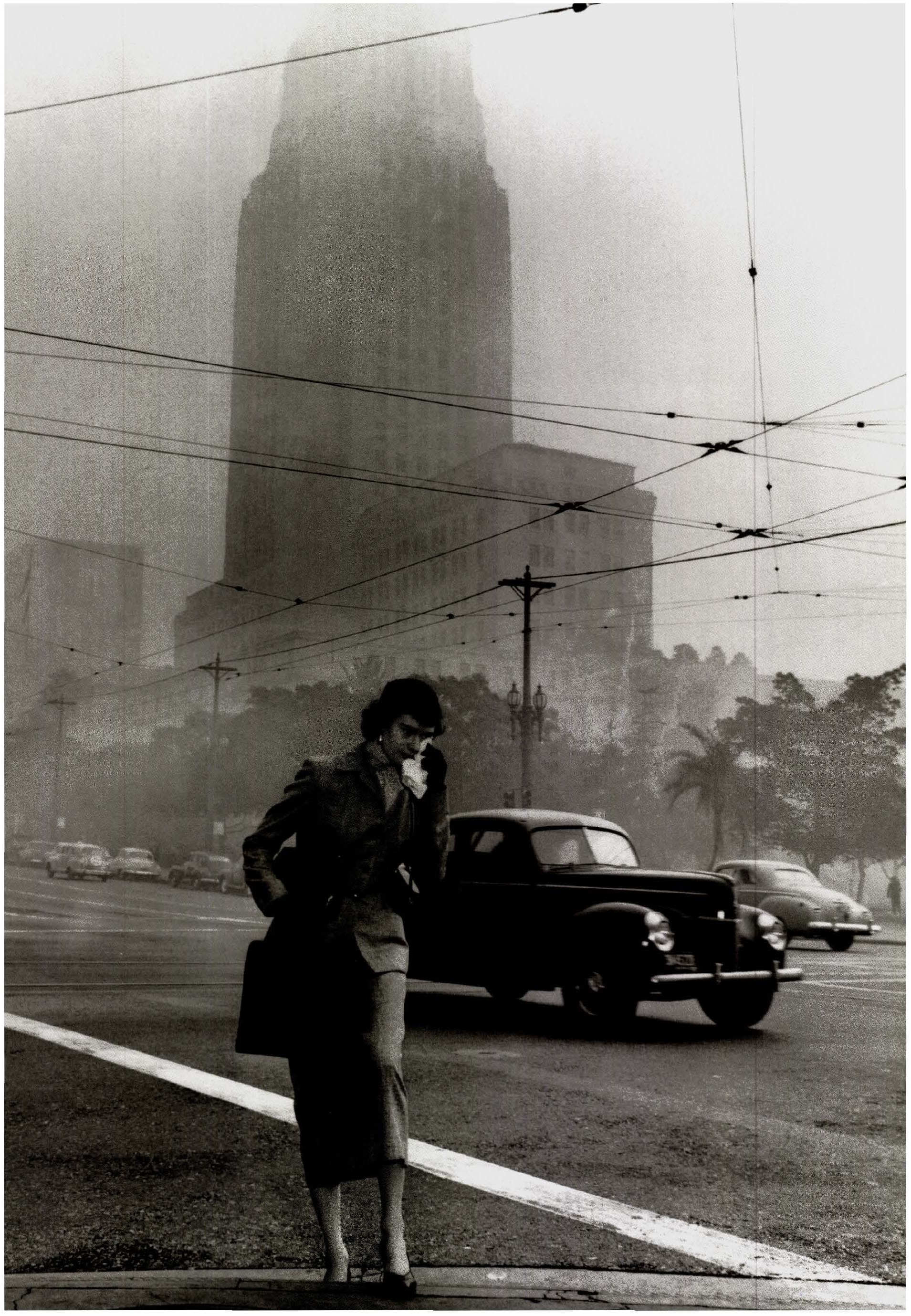
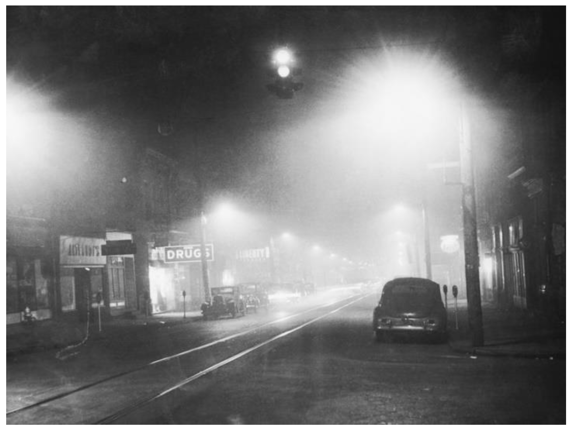
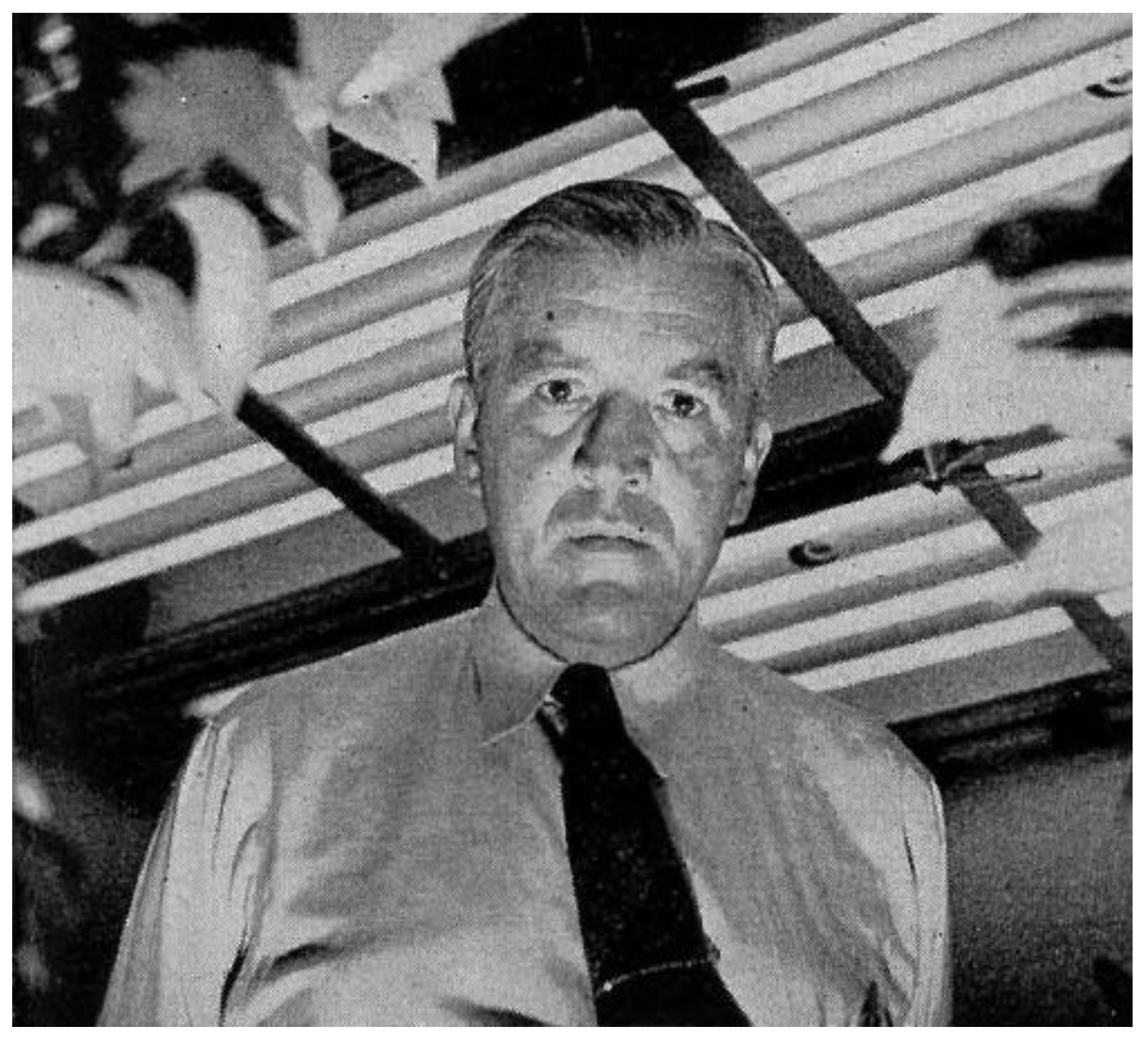
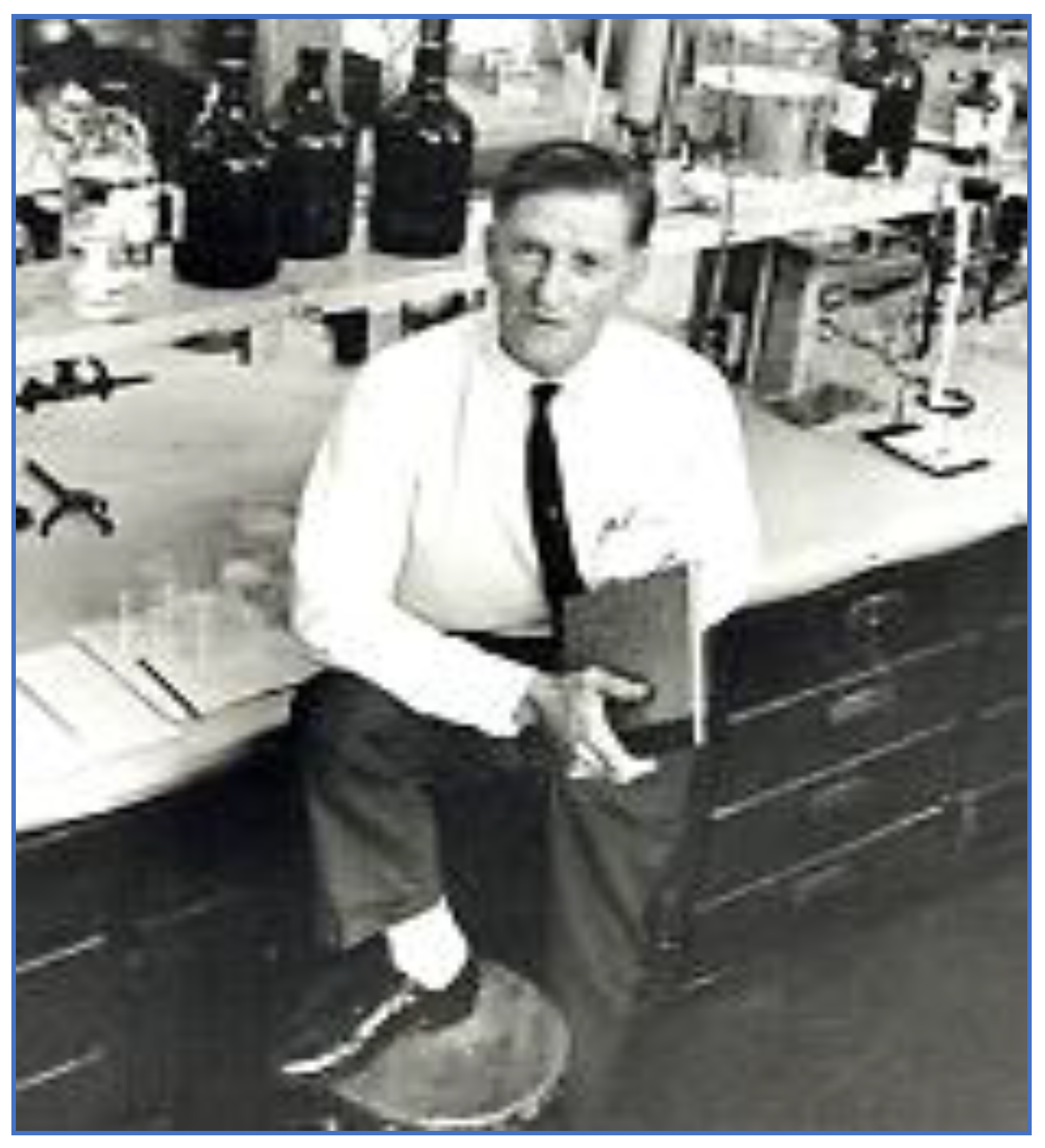
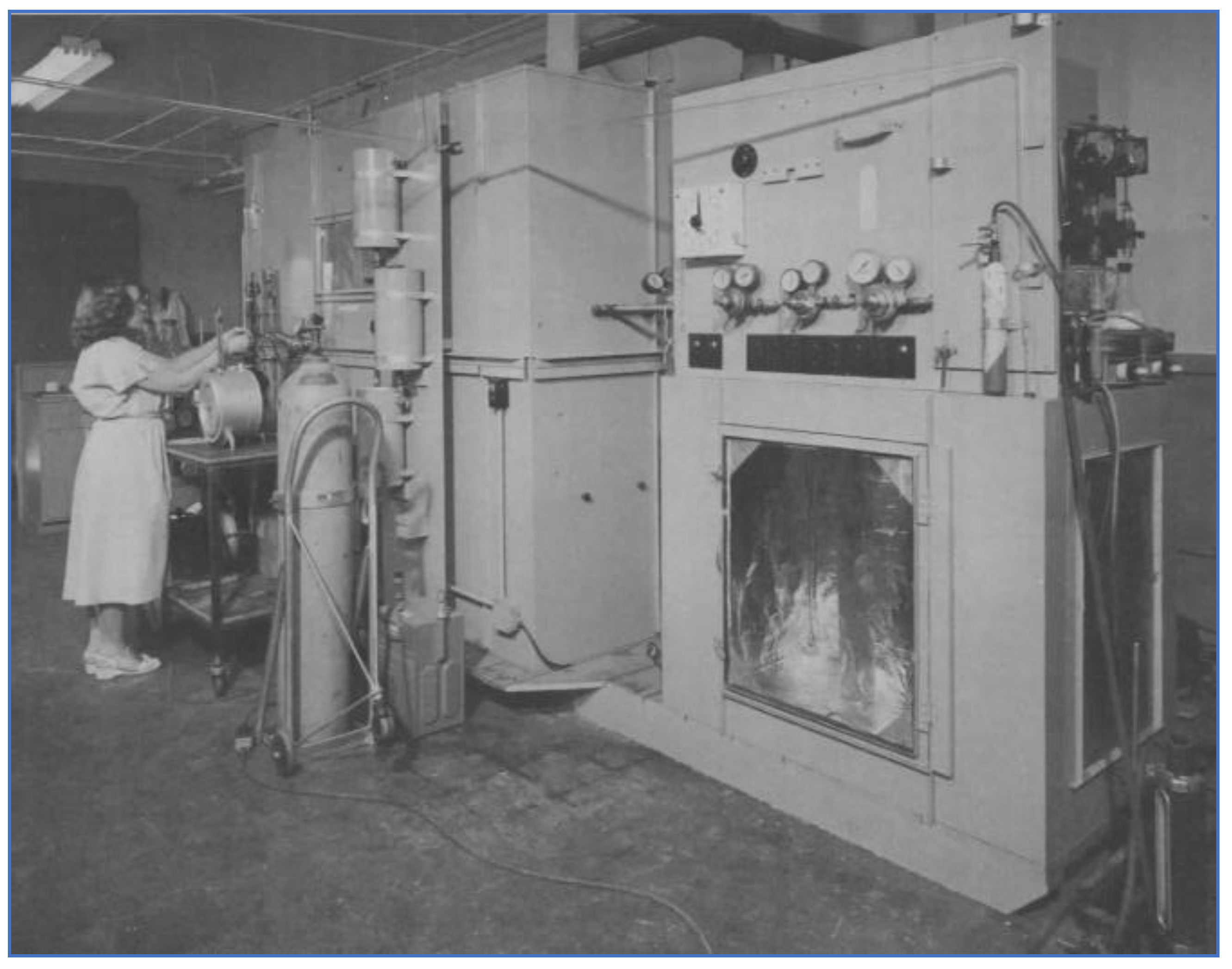
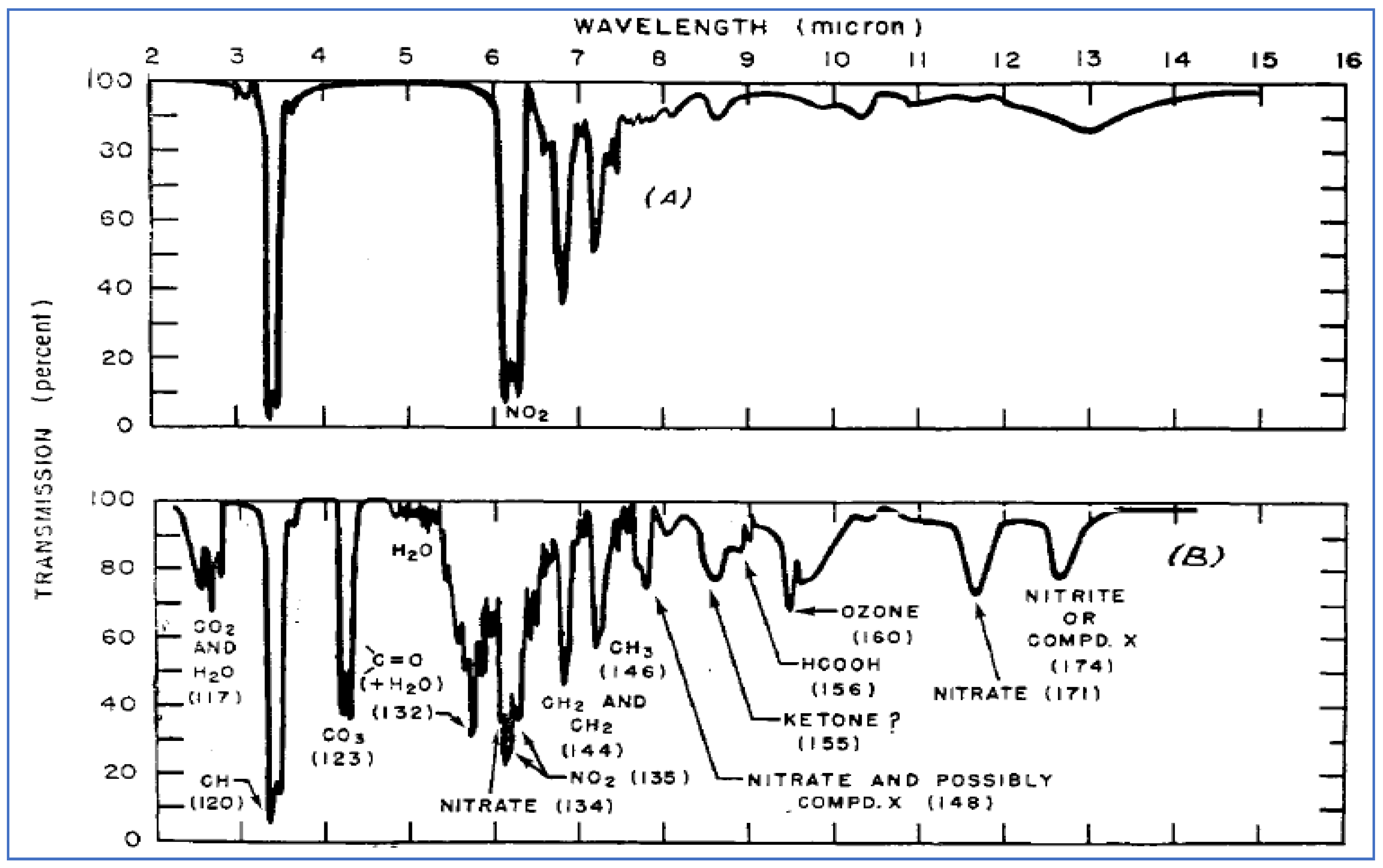
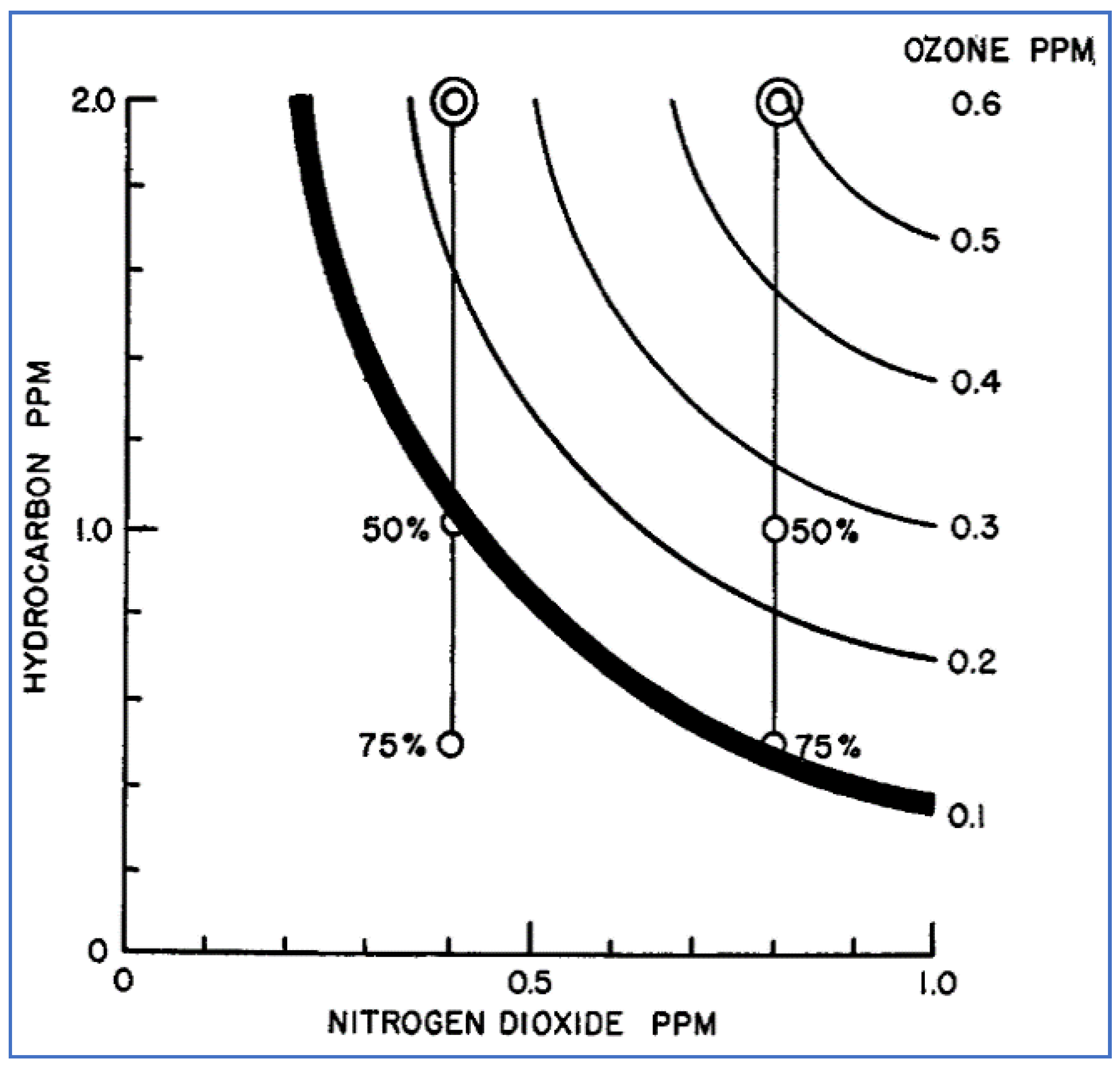
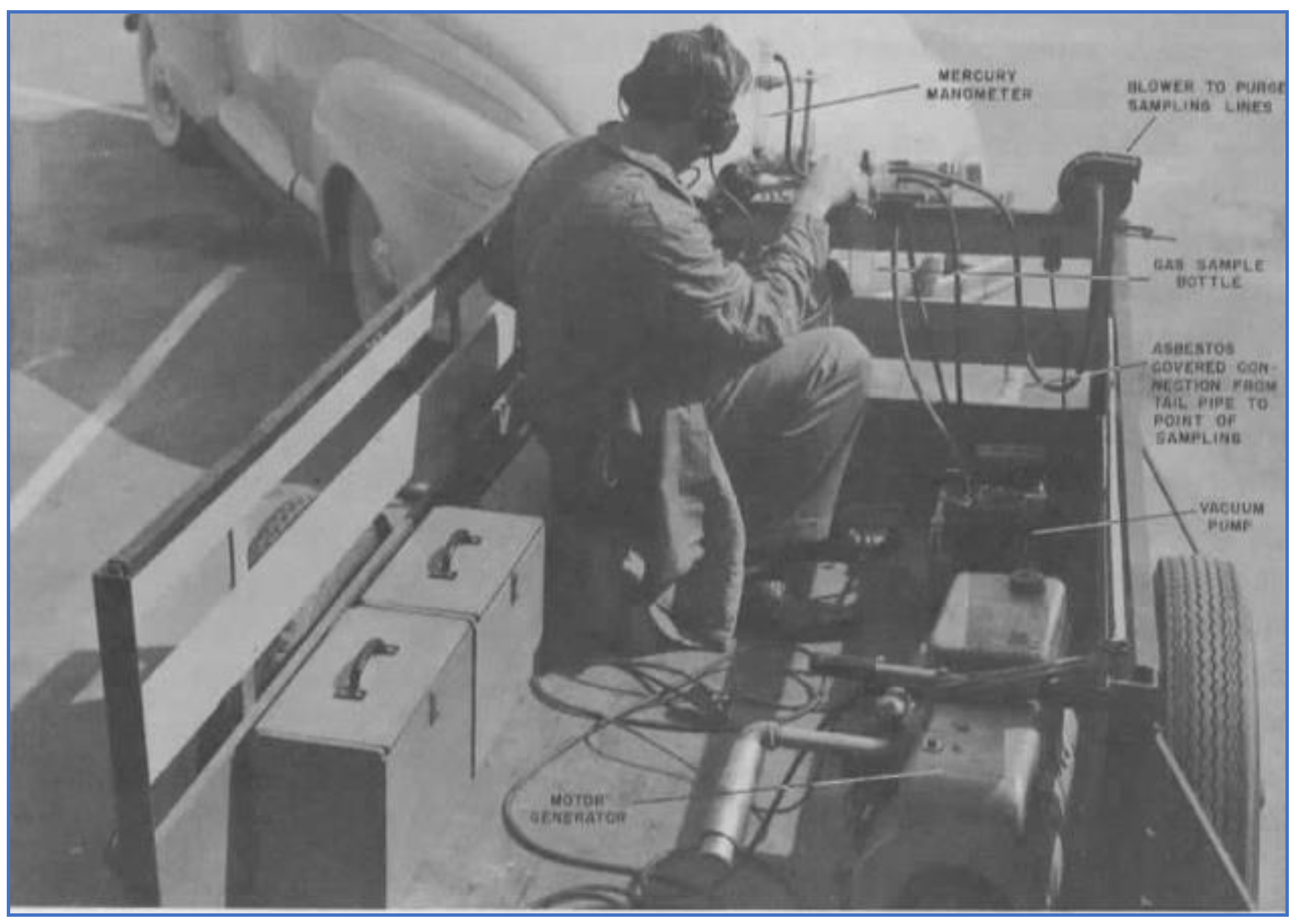
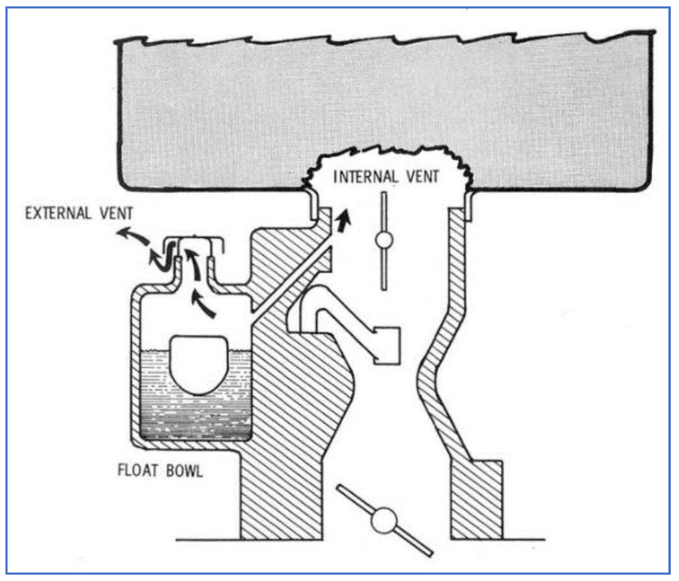
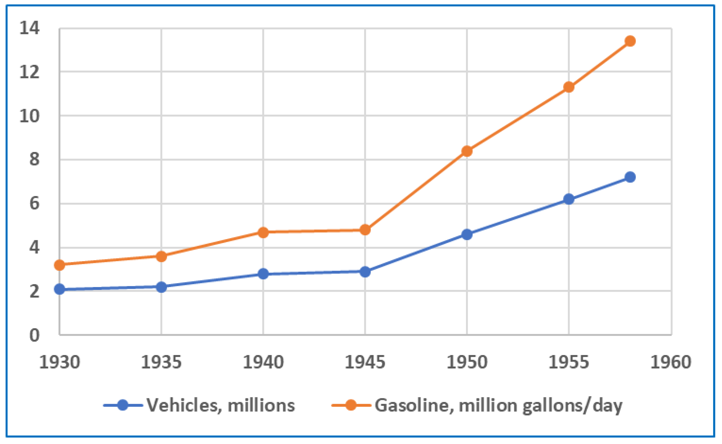
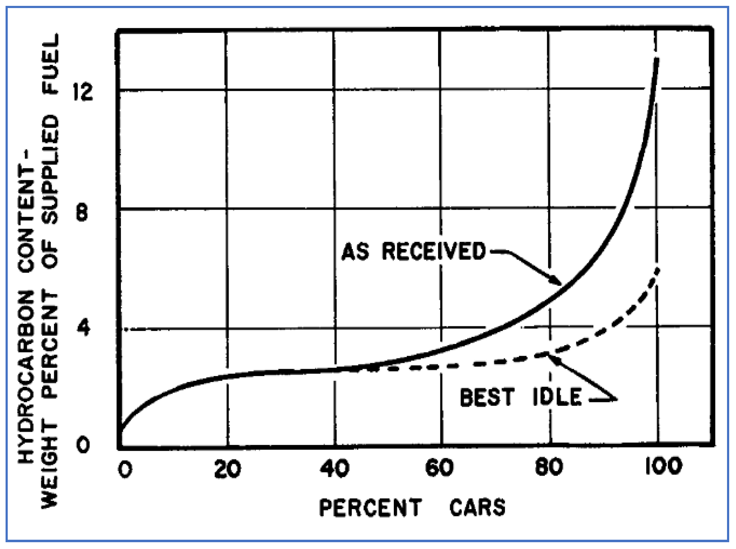
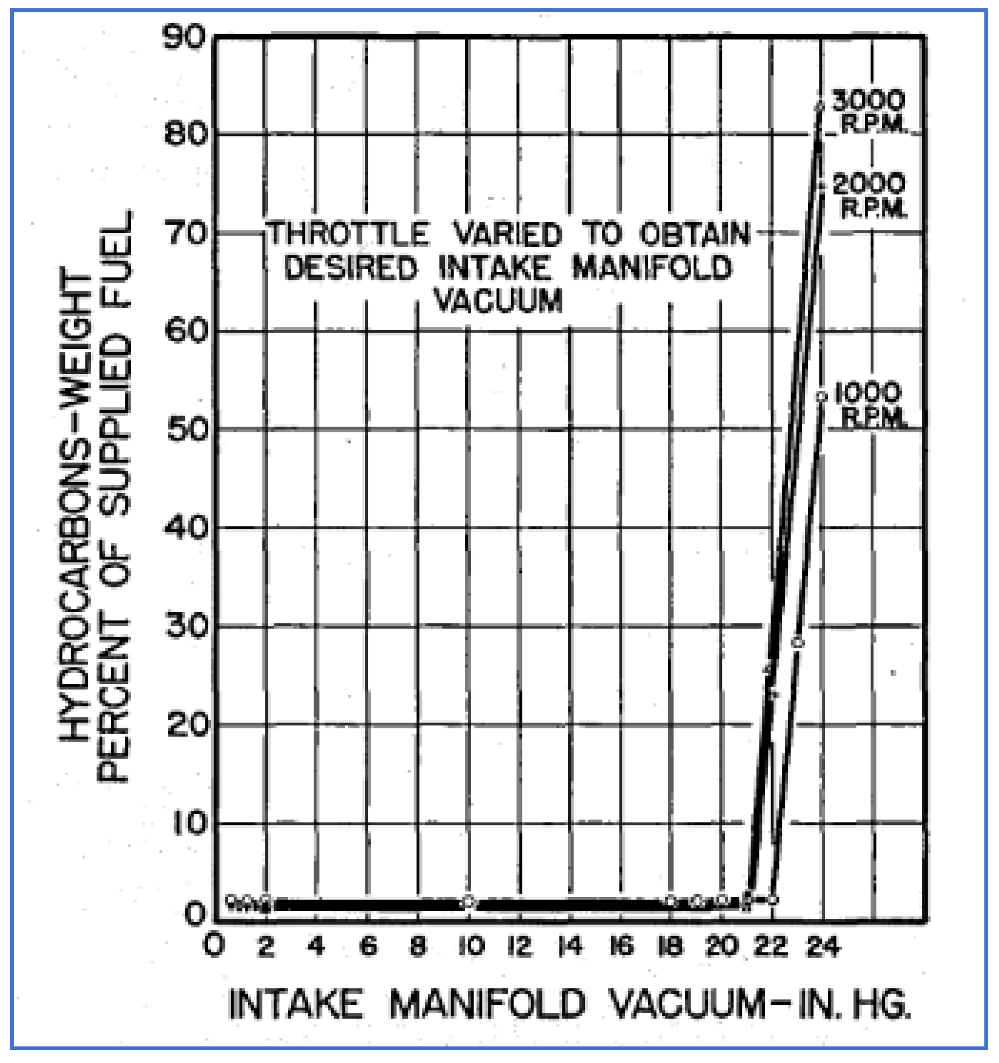
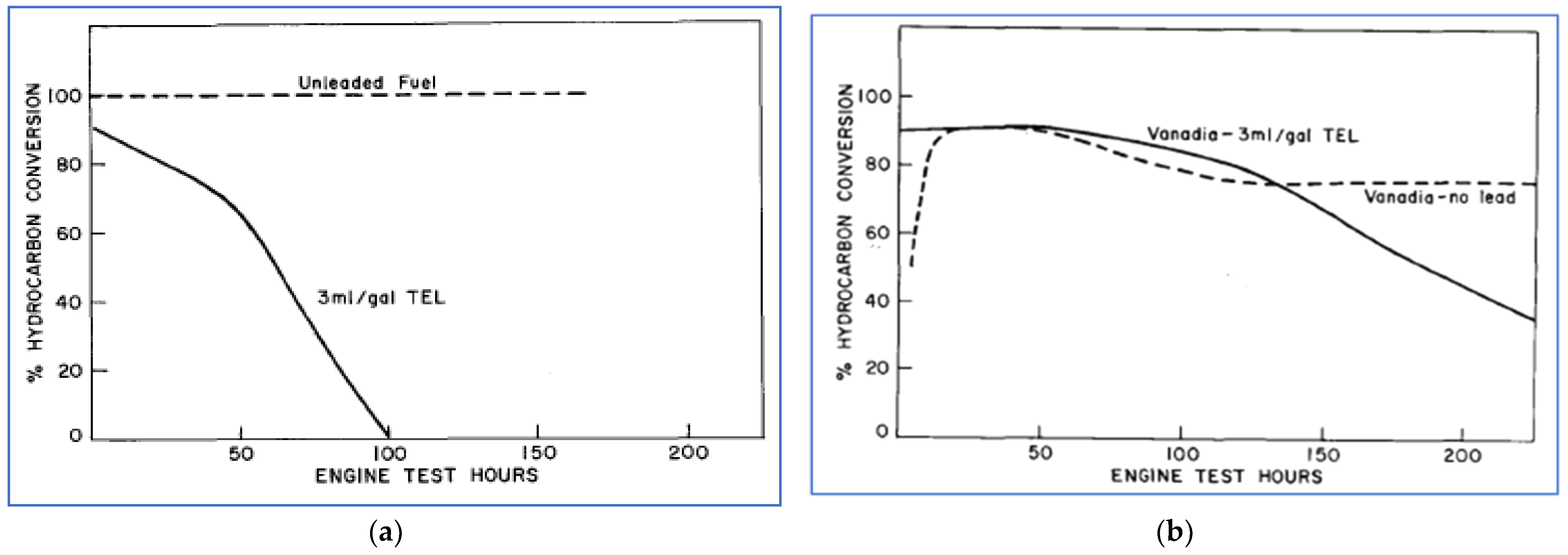
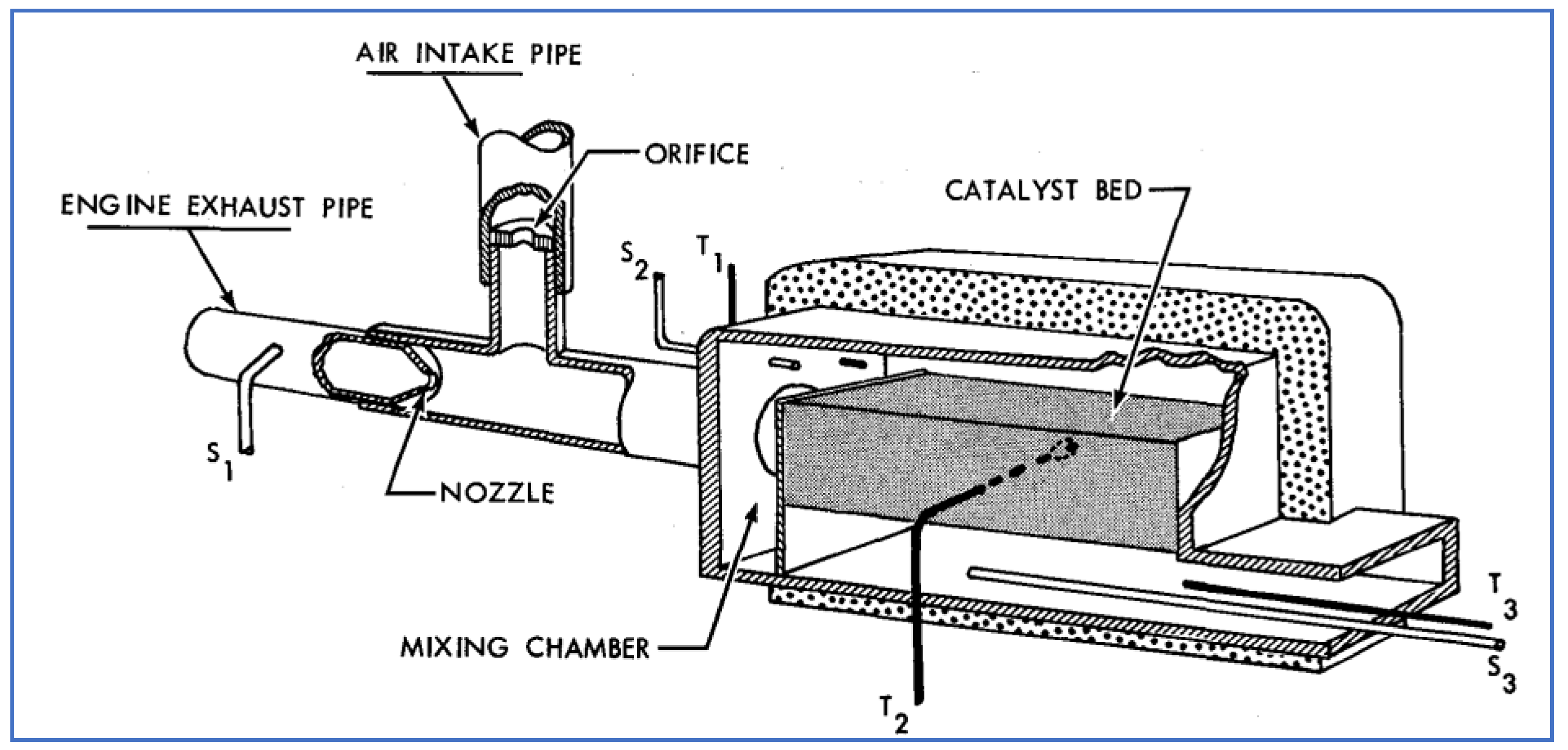
Table 1.
Comparison of Typical London and Los Angeles Types of Smog [4].
Table 1.
Comparison of Typical London and Los Angeles Types of Smog [4].
| London Smog | Los Angeles Smog | |
|---|---|---|
| Chemical components | Particulate matter, sulfur oxides, CO | Hydrocarbons, nitrogen oxides, ozone, CO |
| Fuel sources | Coal, fuel oil | Gasoline, gas, oil |
| Atmospheric conditions | ||
| Winter | Summer, Fall |
| Low (below 40 °F) | High (above 75 °F) |
| High (damp) | Low (dry) |
| Overcast | Bright |
| Ozone concentration | Low | High |
| Time of occurrence | Continuous (day and night) | Daytime only |
| Visibility | Very low (few meters) | Moderate (1/2 mile) |
| Toxicity | Severe bronchial irritation leading to serious illness or death | Eye irritation. No evidence of serious health effects |
Table 2.
Pollutant Concentrations Measured in Downtown LA in 1951 [15].
Table 2.
Pollutant Concentrations Measured in Downtown LA in 1951 [15].
| Gaseous Pollutant | Average Concentration, ppm | |
|---|---|---|
| Days with Good Visibility | Days with Intense Smog | |
| Formaldehyde | 0.04 | 0.09 |
| Other Aldehydes | 0.07 | 0.4 |
| CO | 3.5 | 23.0 |
| Hydrocarbons | 0.2 | 1.1 |
| Total Oxidant | 0.1 | 0.5 |
| Ozone | 0.06 | 0.3 |
| NOx | 0.08 | 0.4 |
| SO2 | 0.05 | 0.3 |
Table 3.
Average vehicle emissions measured in Los Angeles in 1956—CRC Project No. CM-4-58: Comprehensive Exhaust Gas Field Survey [33].
Table 3.
Average vehicle emissions measured in Los Angeles in 1956—CRC Project No. CM-4-58: Comprehensive Exhaust Gas Field Survey [33].
| Driving Condition | HC Emissions a | NOx Emissions b | CO Emissions | ||
|---|---|---|---|---|---|
| lb/hr | % of Fuel Unburned | lb/hr | ppm | Mole % | |
| Idle | 0.32 | 14.4 | 0.001 | 30 | 6.7 |
| Cruise | |||||
| 20 mph | 0.43 | 10.8 | 4.1 | ||
| 30 mph | 0.42 | 9.0 | 0.178 | 905 | 3.3 |
| 40 mph | 0.42 | 7.7 | 2.5 | ||
| 50 mph | 0.87 | 9.4 | 0.577 | 1625 | 1.9 |
| Acceleration | |||||
| 0–60 mph (wide open throttle) | 2.51 | 9.5 | 4.8 | ||
| 0–25 mph (part throttle; 13 s) | 0.99 | 11.4 | 3.7 | ||
| 15–30 mph (part throttle; 11 s) | 0.67 | 9.2 | 0.506 | 1700 | 3.1 |
| Deceleration | |||||
| 50–20 mph (free deceleration) | 0.87 | 40.2 | 0.003 | 60 | |
| 40–20 mph (heavy brake; 5 s) | 0.51 | 23.8 | |||
| 30–0 mph (light brake; 11 s) | 0.49 | 21.1 | |||
| 30–15 mph (light brake; 10 s) | 0.49 | 23.3 | |||
a Measured with Liston-Becker Model 28 NDIR; b calculated as NO2.
Publisher’s Note: MDPI stays neutral with regard to jurisdictional claims in published maps and institutional affiliations. |
© 2021 by the authors. Licensee MDPI, Basel, Switzerland. This article is an open access article distributed under the terms and conditions of the Creative Commons Attribution (CC BY) license (https://creativecommons.org/licenses/by/4.0/).
Share and Cite
MDPI and ACS Style
Hoekman, S.K.; Welstand, J.S. Vehicle Emissions and Air Quality: The Early Years (1940s–1950s). Atmosphere 2021, 12, 1354. https://0-doi-org.brum.beds.ac.uk/10.3390/atmos12101354
AMA Style
Hoekman SK, Welstand JS. Vehicle Emissions and Air Quality: The Early Years (1940s–1950s). Atmosphere. 2021; 12(10):1354. https://0-doi-org.brum.beds.ac.uk/10.3390/atmos12101354
Chicago/Turabian StyleHoekman, S. Kent, and J. Steve Welstand. 2021. "Vehicle Emissions and Air Quality: The Early Years (1940s–1950s)" Atmosphere 12, no. 10: 1354. https://0-doi-org.brum.beds.ac.uk/10.3390/atmos12101354
Note that from the first issue of 2016, this journal uses article numbers instead of page numbers. See further details here.