Objective Calibration of Numerical Weather Prediction Model: Application on Fine Resolution COSMO Model over Switzerland

Abstract

The objective calibration method originally performed on regional climate models is applied to a fine horizontal resolution Numerical Weather Prediction (NWP) model over a mainly continental domain covering the Alpine Arc. The method was implemented on the MeteoSwiss COSMO (consortium for a small-scale modeling) model with a resolution of 0.01° (approximately 1 km). For the model calibration, five tuning parameters of the parameterization schemes affecting turbulence, soil-surface exchange and radiation were chosen. A full year was simulated, with the history of the soil included (hindcast) to find the optimal parameter value. A different year has been used to give an independent assessment of the impact of the optimization process. Although the operational MeteoSwiss model is already a well-tuned configuration, the results showed that a slight model performance gain is obtained by using the Calibration of COSMO (CALMO) methodology.

1. Introduction

Objective calibration of numerical weather prediction (NWP) models refers to a systematic and automatic procedure to improve model quality and quantify sensitivity with potential changes in the parameterization schemes. The need for an objective calibration method stems from the common experience that the NWP model-simulated meteorology exhibits high sensitivity to parameterization changes in certain respects but nonetheless proves difficult to constrain in observations. Therefore, a common practice widely used in state-of-the-art NWP models is tuning, using expert knowledge without following a well-defined strategy [1,2,3,4]. This is also the case in the COSMO model [5], where ‘expert tuning’ is typically made once during the development of the model, for a certain target area, and for a certain model configuration, and is difficult, if not impossible, to replicate.

The calibration approach to substitute tuning relies on a procedure developed originally for global climate models by Neelin et al. [6] and implemented in the regional climate model, COSMO-CLM, in the work of Bellprat et al. [7,8] The main idea of the specific calibration approach is to approximate the model response resulting from parameter perturbations using a computationally efficient statistical regression model (metamodel). The mathematical function at the core of the metamodel is constrained by a minimum set of full model simulations over a time period long enough to represent the variability of the atmospheric conditions. Once fully specified, the metamodel supports a fast sampling of the parameter space to find an optimal combination of the model parameters since the metamodel is computationally efficient, and hence millions of parameter experiments can be conducted. Using an automated approach reduces the risk of compensating errors, as it considers simultaneously a large number of model parameters, observational datasets, and sources of uncertainty.

Based on these works, the priority projects CALMO (Calibration of COSMO model), and consequently CALMO-MAX (CALMO Methodology Applied on extremes), have been integrated within the COSMO consortium, aiming at transferring this method to calibrate the COSMO-NWP model applied in different resolutions [9,10]. A detailed description of the procedure is available in Khain et al. and Voudouri et al. [11,12,13] At the framework of CALMO-MAX, the results of which are presented here, the calibration procedure has been applied to a fine horizontal resolution of 0.01° (approximately 1 km) over a mainly continental domain covering the Alpine Arc, for an entire year and for twenty-one meteorological fields. Calibration is performed using a set of five unconfined model parameters. The selection of parameters is determined by the fields used in the overall performance score, which should be sensitive to the chosen parameters and should reflect the forecaster needs; and finally, the maximum score will indicate the optimal set of parameters. There are several metrics to validate the performance of the NWP model with respect to the model variables considered [14,15]. Validating and calibrating a model using only one variable might be risky, as targeting the improvement of a specific variable (e.g., maximum temperature) might influence the performance of another one; therefore, the selected measure should combine all the meteorological fields affected. The comparative metric (performance score) chosen for this scope in CALMO-MAX was the Global Skill Score called “COSI”, widely used by COSMO since 2007 to judge the long-term trend of the models’ performance [16]. As the goal of the calibration was to improve the quality of daily operational forecasts, the fields considered in the performance score are meteorological quantities used by bench forecasters, such as 2 m temperature, precipitation, dew point temperature and wind speed.

The steps followed in the present work, such as model setup, selection of parameters, sensitivity experiments and performance score, are briefly described in Section 2, while in Section 3 the results of CALMO-MAX applied over Switzerland are discussed. The conclusions are summarized in Section 4.

2. Methodology

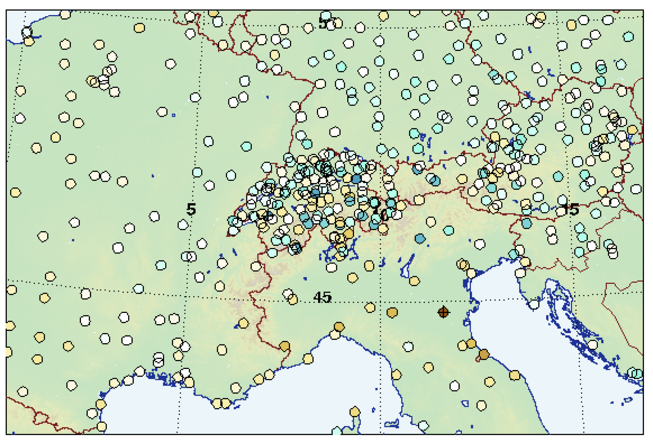
2.1. Model Setup and Observational Data

The NWP model used is the refactored version of COSMO 5.03, capable of running on GPU-based hardware architectures [17], operationally used by MeteoSwiss. Simulations have been performed for two independent years, 2013 mainly for the calibration and 2017 for the validation of the procedure. The model runs with a horizontal resolution of 0.01° (approximately 1 km) over a domain including the Alpine Arc (in particular the wider area of Switzerland and Northern Italy), shown in Figure 1, in the hindcast mode. The grid extends vertically up to 23.5 km (~30 hPa) with 80 model levels. Initial and boundary fields for all tests are provided by the MeteoSwiss operational forecasting archive system. Note also that the soil history is considered for all the CALMO-MAX simulations, and a prior 3 year soil spin-up has been computed using terra standalone (TSA). The model output is constrained toward observations of daily minimum and maximum 2 m temperature, hourly, 6 h and 24 h accumulated precipitation. For temperature, the available measurements of daily mean surface air temperature selected at the dense station network of MeteoSwiss was used. For precipitation, observations over Switzerland were available through the gridded MeteoSwiss radar composites corrected by rain gauges and interpolated to the model grid. Over Northern Italy, observations interpolated to the model grid were used, while over the rest of the simulation domain, the available observations from stations are used (Figure 1). In addition, vertical model profiles at grid points near the sounding locations were considered.

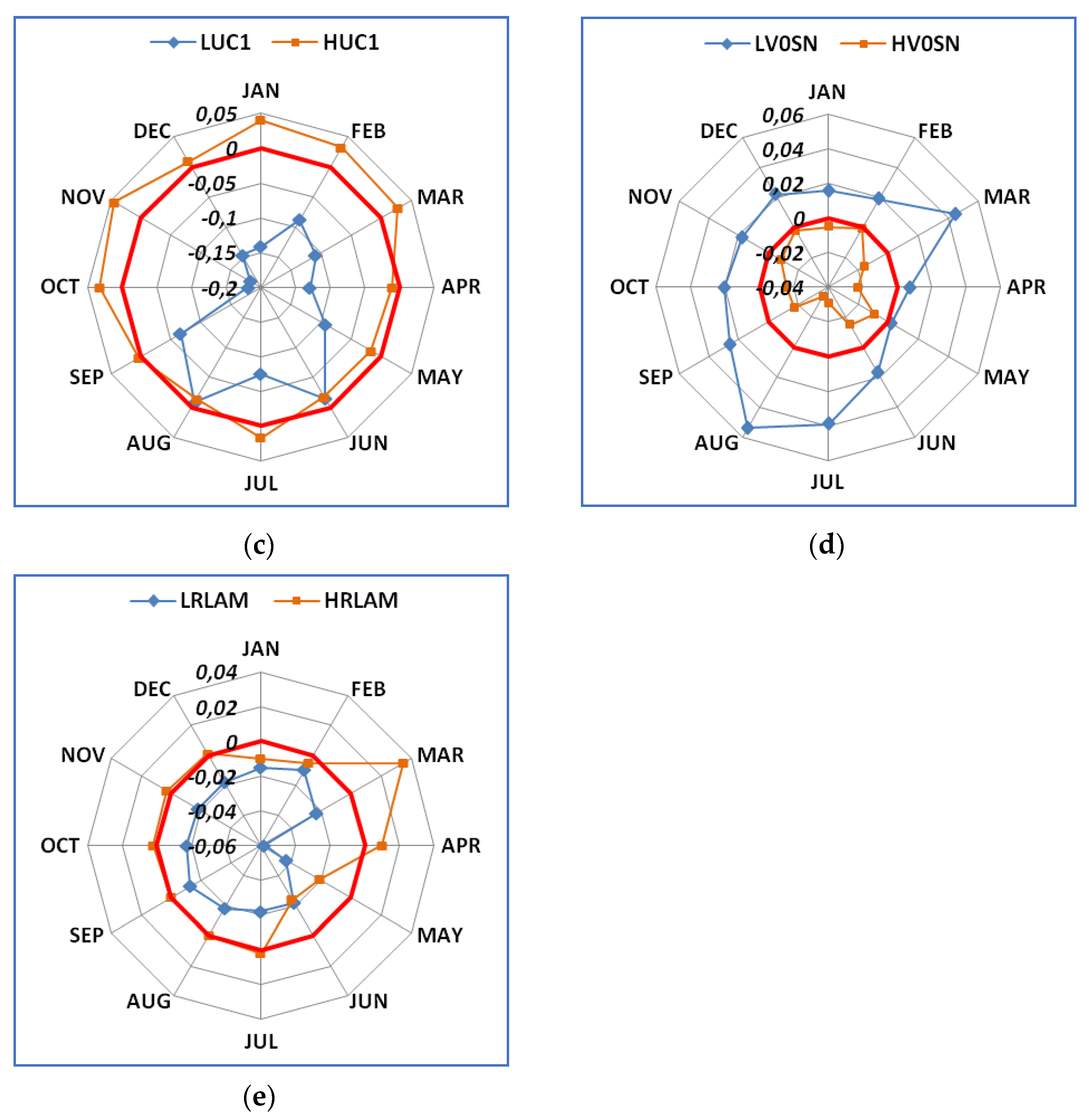
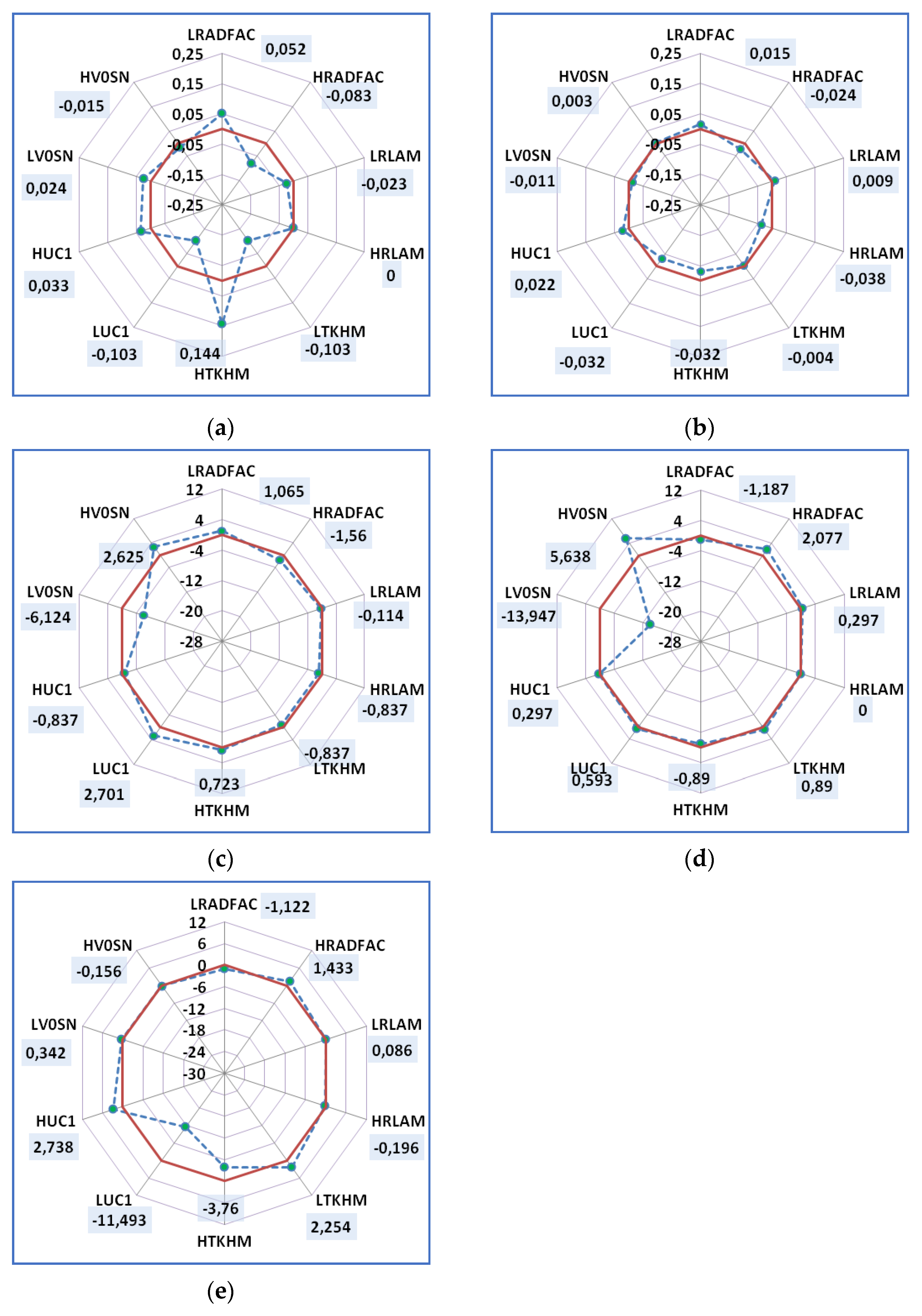
2.2. Sensitivity Experiments

Description of physical processes is achieved through sophisticated parameterization schemes existing in NWP models as COSMO, that often include many unconfined, or ‘free’ parameters, that constitute the list of potential candidates for calibration. These parameters are related to sub-grid scale turbulence, surface layer parameterization, grid-scale cloud formation, moist and shallow convection, precipitation, radiation and soil schemes [18,19].

In the framework of CALMO-MAX, an extended preliminary set of eleven parameters covering turbulence, surface layer parameterization, grid-scale precipitation, moist and shallow convection, radiation and the soil scheme have been tested. Several sensitivity experiments have been performed by Avgoustoglou et al. [20] to define the subset of the most ‘triggering’ parameters for calibration over the Swiss domain. The five model parameters, chosen for CALMO-MAX, are: minimal diffusion coefficients for heat, tkhmin (in m²/s), scalar resistance for the latent and sensible heat fluxes in the laminar surface layer, rlam_heat (no units), factor in the terminal velocity for snow, v0snow(no units), the parameter controlling the vertical variation of critical relative humidity for sub-grid cloud formation, uc1 (no units) and the fraction of cloud water and ice considered by the radiation scheme rad_fac (no units).

Table 1. Parameters used for calibration and their ranges. Default values in bold letters.

Acronym	Parameter/Property	Value
Tkhmin (LTKHM minimum and HTKHM maximum value)	Minimal diffusion coefficient for heat	(0.1, 0.4, 1)
rlam_heat (LRLAM minimum and HRLAM maximum value)	Factor for laminar resistance for heat	(0.1, 1, 2)
uc1 (LUC1 minimum and HUC1 maximum value)	Parameter controlling the vertical variation of critical relative humidity for sub-grid cloud formation	(0, 0.8, 1)
v0snow (LV0SN minimum and HV0SN maximum value)	Factor for vertical velocity of snow	(10, 20, 30)
rad_fac (LRADFAC minimum and HRADFAC maximum value)	Fraction of cloud water and ice considered by the radiation scheme	(0.3, 0.6, 0.9)

summarizes these parameters, while the third column shows their default values (in bold letters) and related ranges (minimum and maximum bound) determined by expert elicitation.

The selection of these unconfined parameters is based on their sensitivity with respect to meteorological fields considered in the performance score, such as 2 m temperature, wind speed and direction, precipitation needed for an everyday forecast, and was tested also over a different domain [21]. Sensitivity of 2 m temperature (in °C) and dew point temperature is expressed as the difference between the 2 m temperature using a test value for a parameter (Ftest) minus the one using the default (proposed by model developers) parameter value (Fdef).

$$\mathrm{S}=\mathrm{Ftest}-\mathrm{Fdef}$$

(1)

Figure 2 summarizes the monthly domain difference of the 2 m temperature for each parameter, namely tkhmin (Figure 2a), rad_fac (Figure 2b), uc1 (Figure 2c), v0snow (Figure 2d) and rlam_heat (Figure 2e). It should be noted that different scales are used; thus, the graph with the largest scale range denotes the most sensitive parameter. The red polygon refers to the zero sensitivity “axis”, where the test value of the parameter gives the same 2 m temperature as the one gained using the default parameter value. Blue and orange lines connect monthly 2 m temperature differences when the parameter takes its minimum, denoted with L in front of the parameter acronym (e.g., LTKHM for tkhmin) and maximum value with H, respectively (e.g, HV0SN for maximum v0snow). As shown in Figure 2a–c, 2 m, the temperature is, as expected, mainly affected by turbulence (represented by tkhmin), where the temperature difference within the parameter range (blue and orange lines) reaches 0.4 °C for December, January and March and by radiation (rad_fac and uc1 parameters) with up to 0.3 °C for April and May, parameterization schemes. On the contrary a low sensitivity of 2 m temperature on grid scale precipitation and surface parameterization scheme is evident, as changing v0snow (factor for vertical velocity for snow) and scalar resistance for the latent and sensible heat fluxes in the laminar surface layer (rlam_heat) gives a maximum temperature difference of 0.09 °C for August (Figure 2d) and only 0.07 °C, for April, respectively (Figure 2e).

Sensitivity experiments on the effect of the five parameters throughout the year have also been performed for several meteorological fields and these yearly sensitivities for 2 m temperature, dew point temperature, 24 h accumulated precipitation (kg m⁻²), 24 h accumulated grid-scale snow (kg m⁻²) and hourly total cloud cover average (%) are illustrated in Figure 3a–e, respectively. As in Figure 2, the red polygon refers to the zero sensitivity “axis”. The sensitivities for each parameter are depicted with green bullets, where H and L stand for maximum and minimum parameter values. The dashed polygon line that connects the dots denotes optically the overall sensitivity for the considered meteorological variable, especially to the degree that it is convex/concave and mainly in reference to the zero-sensitivity red polygon. Different scales are used, as for 2 m temperature, and dew point temperature sensitivities (calculated using Equation (1)) are in °C, while for precipitation, snow and total cloud cover, sensitivities are expressed as a percentage. Sensitivity values (S) on the spider graphs for precipitation, snow and total cloud cover are defined as:

$$\mathrm{S}(\%)=\frac{\mathrm{Ftest}-\mathrm{Fdef}}{\mathrm{Fdef}}100$$

(2)

where Ftest is the meteorological field value (precipitation, snow, total cloud cover) when a test value of the parameter considered is used and Fdef represents its default parameter value. Similarly to the monthly sensitivity shown in Figure 2, 2 m temperature, changes up to 0.25 °C throughout the year and is affected mainly by tkhmin and rad_fac and uc1 (Figure 3a). Dew point temperature is less sensitive than 2 m temperature to these five parameters (as the same scale is used), with higher differences being 0.05 °C for rlam_heat, rad_fac and uc1 as shown in Figure 3b. Precipitation is affected by changes in rad_fac, uc1 and also v0snow up to 8% (Figure 3c), while for v0snow, different values leverage, as expected, with snow up to 20% (Figure 3d). Hourly average total cloud differs up to 14% when changing uc1, namely the parameter associated with sub-grid cloud formation (Figure 3e).

2.3. The Performance Score

Once the meta-model is fitted, it can be used as a surrogate to perform a large number of simulations, testing several parameter values in order to find the optimum ones. The goal is to use the meta-model to obtain the highest performance score, which indicates the optimal set of parameters. Thus, the definition of a suitable metric (i.e., the performance score) capable of overall validatation of the quality of the model output is a key element in the calibration method. The performance score (PS) applied in this work is based on a modification of COSMO Index (COSI) [16] to reflect changes in the model performance associated with more meteorological fields rather than the ones originally used. The PS used combines meteorological fields such as daily 2 m temperature, maximum (Tmax) and minimum 2 m temperature (Tmin); 24 h accumulated precipitation (Pr), and sixteen fields, whose observations can be provided by soundings, that is: Total column water vapor (TCWV); Vector wind shear between the levels of 500 mb and 700 mb (WS1); Vector wind shear between the levels of 700 mb and 850 mb (WS2); Vector wind shear between the levels of 850 mb and 1000 mb (WS3); Temperatures at 500 mb (T500), 700 mb (T700) and 850 mb (T850) respectively; Relative humidity at 500 mb (RH500), 700 mb (RH700) and 850 mb RH850) respectively; East-west wind component at 500 mb (U500), 700 mb (U700) and 850 mb (U850) respectively; South-north wind component at 500 mb (V500), 700 mb (V700) and 850 mb (V850). The equation of the PS (already used in CALMO-MAX) has been presented in Voudouri et al. [12] Negative PS is associated with a reduction in the performance, while positive PS indicates an improvement in the performance of the model attributed to the ‘optimum’ parameter values replacing the default ones.

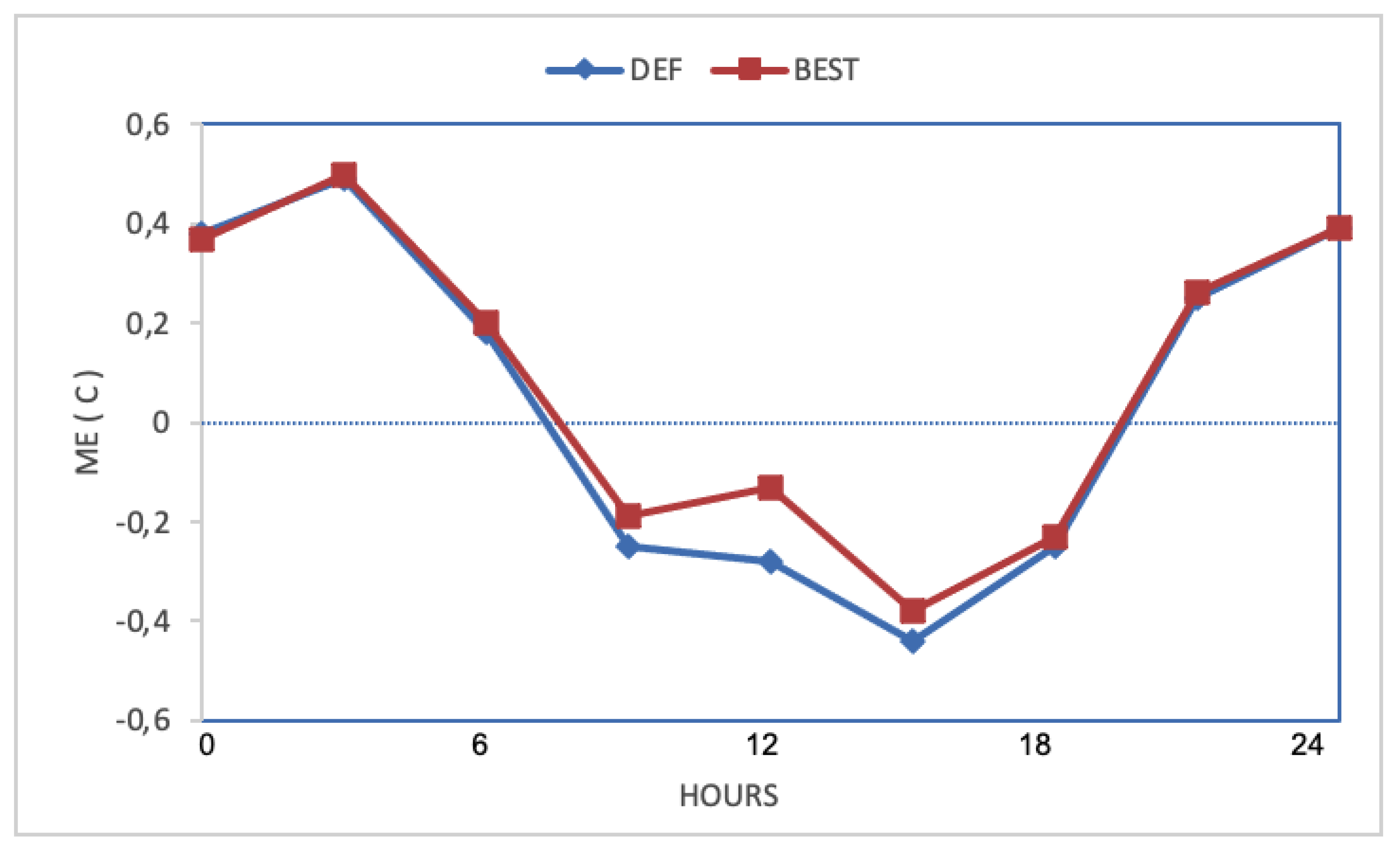
3. Results and Discussion

In this section, the results obtained in the frame of CALMO-MAX are presented.The MeteoSwiss COSMO-1 configuration at 0.01° resolution has been calibrated, selecting the five model parameters described in Section 2, using a full year statistic, to demonstrate the benefits of the methodology. The year 2013 has been chosen as climatologically representative of the target area. A different year, that is 2017, has also been used to have an independent assessment of the impact of the optimization process.

The minimum number of simulations for the N parameters to fit the meta-model is according to Neelin et al. [6], 1 + 2N + N (N − 1)/2. Therefore, for 5 parameters 21 model runs have been performed for 2013 to determine the optimum set of these parameters. It should be noted that although the calibration is performed over the entire year, optimum parameter values are extracted over sets of 10-day periods. An average for these 36 periods is then produced to extract the best optimum parameter set over the entire year. The optimum parameter values were extracted as follows: tkhmin = 0.279 (m²/s), rlam_heat = 0.929, v0snow = 18.95, rad_fac = 0.6775 and uc1 = 0.7686. The default parameter values were replaced by these “optimal” values, and model simulations for 2013 have been performed again to investigate the improvement in model performance. Additionally, simulations for 2017 have been performed to examine whether the optimum parameter set, calculated for the year of the calibration, is also beneficial for a different independent year.

The verification of simulations using default parameter values (tkhmin = 0.4 (m²/s), rlam_heat = 1, v0snow = 20, rad_fac = 0.6 and uc1 = 0.8) (DEF) against the one using optimum parameter set (BEST) for 2 m temperature, dew point temperature and 10 m wind speed are presented in

Table 2. Statistics of selected meteorological fields for 2013 and 2017.

Parameter	T2 m (°C)				Td (°C)				10 m Wind Speed (m/s)
Year	2013		2017		2013		2017		2013		2017
Measure/Simulation	DEF	BEST	DEF	BEST	DEF	BEST	DEF	BEST	DEF	BEST	DEF	BEST
ME	0.01	0.04	0.18	0.09	0.06	−0.01	−0.029	−0.029	0.13	0.11	0.115	0.104
RMSE	2.07	2.07	2.22	2.21	2.31	2.33	2.37	2.36	1.9	1.9	1.955	1.954
MINOBS	−30.7		−29.6		−73		−54.8		0		0
MINMOD	−28.6	−28.5	−30.2	−30.0	−37.48	−38.67	−44.41	−45.47	0.007	0.001	0.0012	0.0013
MAXOBS	40.8		42		39		41.2		46		40.1
MAXMOD	42.7	42.6	44.03	43.38	25.24	25.77	24.86	25.00	29	29	28.19	28.04

for 2013 and 2017, over the entire simulation domain. More specifically, statistical measures such as mean error (ME), root mean square error (RMSE), minimum (MINMOD) and maximum (MAXMOD) model values, minimum (MINOBS) and maximum (MAXOBS) observed values are shown. According to the statistics of Table 2, BEST configuration allows a decrease in dew point temperature and 10 m wind speed for 2013 and 2017, while there is a small increase of 2 m temperature in 2013. However, there is an overall balance between the minimum and maximum modeled temperature values compared to the observed ones, which is 0.1 °C closer to the observed minimum when using default parameter values and is equally close to the maximum observed temperature when using the optimum ones.

In addition, a comparison of the daily cycle (averaged over the entire year and entire model domain) of 2 m temperature ME when using the default (blue line) and optimum (red line) parameter values for 2013 are shown in Figure 4. An improvement is evident, as there is a decrease in ME of 0.1 °C during daytime when substituting default parameter values with the optimum ones. The maximum and minimum dew point temperature calculated using the optimum parameter set is closer to the observed ones for 2013 and 2017.

A decrease in the ME of the 2 m temperature is observed when using the optimized configuration, which is 0.09 °C instead of 0.18 °C for 2017, as shown in Table 2. This is also the case for 10 m wind speed, with ME equal to 0.104 m/s against 0.115 m/s, while the dew point temperature ME remains stable and there is also a small improvement of approximately 0.01 °C in RMSE of 2 m temperature for 2017. Thus, the calibration procedure objectively provides a value of a ‘free’ parameter other than the one subjectively defined by the model developers that gives equally good model results and also slightly improves the model performance.

4. Conclusions

Τhe implementation and consolidation of an objective calibration method on the fine resolution COSMO model over the MeteoSwiss operational domain has been examined at the framework of the CALMO-MAX project. A limited number of parameters that are associated with the main parameterization schemes affecting turbulence, soil-surface exchange and radiation has been used for the calibration. The impact of the optimization process on 2 m temperature, dew point temperature and 10 m wind speed has been investigated not only for the base year of the calibration, but also for a different year to have an independent assessment. Although the results presented showed only a slight model performance gain obtained using the specific methodology, the fact that the chosen model configuration is based on the operational model of MeteoSwiss should be considered. The specific model configuration is close to the DWD configuration, an already well-tuned configuration by model developers. In addition an improvement is evident for the year 2017 and is used for the independent assessment, indicating that the determined as optimum parameter values for 2013 are also valid for 2017.

It should be noted that this objective calibration methodology could have a signifcant impact on the future development of NWP models. More specifically, once the computational cost is reduced, the developed methodology could be used by any NWP model to define an optimal calibration over the target area of interest, for re-calibration after major model changes (e.g., different horizontal and/or vertical resolution) and for an unbiased assessment of different modules (e.g., parameterization schemes), as well as for optimal perturbation of parameters when run in ensemble mode.

Furthermore, a better understanding of the sensitivity of the model quality associated with a specific parameter value, as provided by the meta-model, could benefit the quantification of the flow-dependent model forecast and could clarify the impact of a specific parameter on the overall model performance.

References

1. Duan, Q.; Schaake, J.; Andreássian, V.; Franks, S.; Goteti, G.; Gupta, H.V.; Gusev, Y.M.; Habets, F.; Hall, A.; Hay, L.; et al. Model Parameter Estimation Experiment (MOPEX): An overview of science strategy and major results from the second and third workshops. J. Hydrol. 2006, 320, 3–17. [Google Scholar] [CrossRef] [Green Version]
2. Duan, Q.; Di, Z.; Quan, J.; Wang, C.; Gong, W.; Gan, Y.; Fan, S. Automatic model calibration—A new way to improve numerical weather forecasting. Bull. Am. Meteorol. Soc. 2016, 98, 959–970. [Google Scholar] [CrossRef]
3. Skamarock, W.C. Evaluating Mesoscale NWP Models Using Kinetic Energy Spectra. Mon. Wea. Rev. 2004, 132, 3019–3032. [Google Scholar] [CrossRef]
4. Bayler, C.; Gail, M.; Aune, R.M.; Raymond, W.H. NWP Cloud Initialization Using GOES Sounder Data and Improved Modeling of Non precipitating Clouds. Mon. Wea. Rev. 2000, 128, 3911–3921. [Google Scholar] [CrossRef]
5. Available online: http://cosmo-model.org/content/model/documentation/core/cosmo_physics_5.05.pdf (accessed on 10 October 2021).
6. Neelin, J.D.; Bracco, A.; Luo, H.; McWilliams, J.C.; Meyerson, J.E. Considerations for parameter optimization and sensitivity in climate models. Proc. Natl. Acad. Sci. USA 2010, 107, 21349–21354. [Google Scholar] [CrossRef] [PubMed] [Green Version]
7. Bellprat, O.; Kotlarski, S.; Lüthi, D.; Schär, C. Objective calibration of regional climate models. J. Geophys. Res. 2012, 117, D23115. [Google Scholar] [CrossRef] [Green Version]
8. Bellprat, O.; Kotlarski, S.; Lüthi, D.; Schär, C. Exploring perturbed physics ensembles in a regional climate model. J. Clim. 2012, 25, 4582–4599. [Google Scholar] [CrossRef]
9. Voudouri, A.; Khain, P.; Carmona, I.; Bellprat, O.; Grazzini, F.; Avgoustoglou, E.; Bettems, J.M.; Kaufmann, P. Objective calibration of numerical weather prediction models. Atmos. Res. 2017, 190, 128–140. [Google Scholar] [CrossRef]
10. Voudouri, A.; Khain, P.; Carmona, I.; Avgoustoglou, E.; Bettems, J.M.; Grazzini, F.; Bellprat, O.; Kaufmann, P.; Bucchignani, E. Calibration of COSMO Model, Priority Project CALMO, Final Report; COSMO Technical Report: 2017; DWD: Offenbach, Germany, 2017; Volume 32. Available online: http://cosmo-model.org/content/model/documentation/techReports/cosmo/docs/techReport32.pdf (accessed on 10 October 2021).
11. Khain, P.; Carmona, I.; Voudouri, A.; Avgoustoglou, E.; Bettems, J.-M.; Grazzini, F. The Proof of the Parameters Calibration Method: CALMO Progress Report; COSMO Technical Report: 2015; DWD: Offenbach, Germany, 2015; Volume 25. Available online: http://cosmo-model.org/content/model/documentation/techReports/cosmo/docs/techReport25.pdf (accessed on 10 October 2021).
12. Khain, P.; Carmona, I.; Voudouri, A.; Avgoustoglou, E.; Bettems, J.-M.; Grazzini, F.; Kaufman, P. CALMO Progress Report; COSMO Technical Report: 2017; DWD: Offenbach, Germany, 2017; Volume 31. Available online: http://cosmo-model.org/content/model/documentation/techReports/cosmo/docs/techReport31.pdf (accessed on 10 October 2021).
13. Voudouri, A.; Khain, P.; Carmona, I.; Avgoustoglou, E.; Kaufmann, P.; Grazzini, F.; Bettems, J.M. Optimization of high resolution COSMO model performance over Switzerland and Northern Italy. Atmos. Res. 2018, 213, 70–85. [Google Scholar] [CrossRef]
14. Murphy, A.H. Skill Scores Based on the Mean Square Error and Their Relationships to the Correlation Coefficient. Mon. Weat. Rev. 1988, 116, 2417–2424. [Google Scholar] [CrossRef]
15. Wilks, D.S. Statistical Methods in the Atmospheric Sciences; Academic Press: San Diego, CA, USA, 1995; p. 467. [Google Scholar]
16. Damrath, U. Long-term trends of the quality of COSMO-EU forecast expressed as the universal score COSI and others scores for temperature 2 m and wind 10 m—Related to A global score for COSMO models. In Proceedings of the Recommendations from “The Score Meeting of 20th August 2007 in Zurich” 11th COSMO-GM, Offenbach, Germany, 7–11 September 2009. [Google Scholar]
17. Lapillonne, X.; Fuhrer, O. Using compiler directives to port large scientific applications to GPUs: An example from atmospheric science. Parallel Process. Lett. 2014, 24, 1450003. [Google Scholar] [CrossRef]
18. Doms, G.; Foerstner, J.; Heise, E.; Herzog, H.-J.; Mironov, D.; Raschendorfer, M.; Reinhardt, T.; Ritter, B.; Schrodin, R.; Schultz, J.-P.; et al. A Description of the Nonhydrostatic Regional COSMO Model. Part II: Physical Parameterization; DWD: Offenbach, Germany, 2011. Available online: http://www.cosmo-model.org/content/model/documentation/core/cosmo_physics_4.20.pdf (accessed on 10 October 2021).
19. Gebhardt, C.; Theis, S.E.; Paulat, M.; Ben, Z. Bouallègue Uncertainties in COSMO-DE precipitation forecasts introduced by model perturbations and variation of lateral boundaries. Atmos. Res. 2011, 100, 168–177. [Google Scholar] [CrossRef]
20. Avgoustoglou, E.; Voudouri, A.; Carmona, I.; Bucchignani, E.; Levi, Y.; Bettems, J.-M. A Methodology towards the Hierarchy of COSMO Parameter Calibration Tests via the Domain Sensitivity over the Mediterranean Area; COSMO Technical Report: 2020; DWD: Offenbach, Germany, 2020; Volume 42. Available online: http://cosmo-model.org/content/model/documentation/techReports/cosmo/docs/techReport42.pdf (accessed on 10 October 2021).
21. Bucchignani, E.; Voudouri, A.; Mercogliano, P. A Sensitivity Analysis with COSMO-LM at 1 km Resolution over South Italy. Atmosphere 2020, 11, 430. [Google Scholar] [CrossRef] [Green Version]
Figure 1. Simulation domain and distribution of stations used for calibration.
Atmosphere 12 01358 g001
Figure 2. Monthly sensitivity of 2 m temperature for (a) tkhmin, (b) rad_fac (c) uc1 (d) v0snow and (e) rlam-heat per month for year 2013. The blue line represents the lowest (L) value and the orange line represents the highest (H) value of each parameter, while the other parameters are kept within their default values. The red circle denotes the referenced default value (the zero °C circle).
Atmosphere 12 01358 g002aAtmosphere 12 01358 g002b
Figure 3. Yearly sensitivity of (a) 2 m temperature, (b) dew point temperature (c) precipitation (d) snow and (e) total cloud cover with respect to all selected parameters for the year 2013.
Atmosphere 12 01358 g003
Figure 4. Daily cycle (averaged over the entire year and entire model domain) of 2 m temperature ME when using default (blue line) and optimum (red line) parameter values for 2013.
Atmosphere 12 01358 g004