Diagnosis of Atmospheric Drivers of High-Latitude Evapotranspiration Using Structural Equation Modeling

Abstract

Evapotranspiration (ET) is a relevant component of the surface moisture budget and is associated with different drivers. The interrelated drivers cause variations at daily to interannual timescales. This study uses structural equation modeling to diagnose the drivers over an ensemble of 45 high-latitude sites, each of which provides at least several years of in situ measurements, including latent heat fluxes derived from eddy covariance flux towers. The sites are grouped by vegetation type (tundra, forest) and the presence or absence of permafrost to determine how the relative importance of different drivers depends on land surface characteristics. Factor analysis is used to quantify the common variance among the variables, while a path analysis procedure is used to assess the independent contributions of different variables. The variability of ET at forest sites generally shows a stronger dependence on relative humidity, while ET at tundra sites is more temperature-limited than moisture-limited. The path analysis shows that ET has a stronger direct correlation with solar radiation than with any other measured variable. Wind speed has the largest independent contribution to ET variability. The independent contribution of solar radiation is smaller because solar radiation also affects ET through various other drivers. The independent contribution of wind speed is especially apparent at forest wetland sites. For both tundra and forest vegetation, temperature loads higher on the first factor when permafrost is present, implying that ET will become less sensitive to temperature as permafrost thaws.

1. Introduction

The terrestrial surface moisture budget has three main components: precipitation (P), evapotranspiration (ET), and runoff (R). While precipitation is the primary driver of changes in the other two components as well as changes in soil moisture storage, ET is a key determinant of soil moisture, especially in the upper soil layers, over timescales of days to seasons. However, rates of ET are affected by other factors in addition to precipitation: incoming radiation and the ground temperature, the dryness of the air, wind speed, vegetation type, and the availability of moisture in the upper soil layers [1,2]. In high latitudes, the situation is further complicated by the freeze–thaw status of the ground [3,4]. Much of the Arctic and subarctic is underlain by permafrost, which is characterized by an active layer that thaws seasonally from the surface to depths of as much as a meter or two [5]. Even high-latitude land areas without permafrost experience a seasonal freeze of the upper soil column, and the duration of the seasonal freeze can exceed six months. Finally, snow cover is a pervasive feature of the high-latitude terrestrial region and a substantial contributor to the lateral discharge (runoff) [6].

Drivers of evapotranspiration in the Arctic have been identified in several previous studies of the high-latitude surface moisture budget [1,7,8]. It is known that ET increases as relative humidity decreases, and this relationship is captured by the bulk transfer formulations used in many climate models [9]. Dependencies of ET on solar radiation, temperature and relative humidity are consistent with the elevated values of ET during warm and dry conditions [7,10]. Previous work also suggests that the role of temperature in the overall variability of ET may have a relationship with permafrost. The authors of [11] describe how permafrost acts as a buffer in partitioning energy into atmospheric and ground heat fluxes. This buffer can impact the responses of thermal variables such as surface air temperature to increased solar radiation during the warm season.

Various studies have found strong correlations between atmospheric humidity and ET in boreal forest ecosystems. For example, [12] showed that woodland ecosystems in northern high latitudes are correlated with vapor pressure deficit (VPD), radiation, and temperature. The transpiration component of ET in birch forests showed an especially strong connection to VPD, which is directly related to relative humidity. Studies such as [13,14,15,16] have shown a linkage between VPD and ET, while [17] constructed a relative-humidity-based ET model for various locations in the contiguous United States.

Eddy covariance measurements of the latent heat flux (LHF) were used by the authors of [18] to evaluate variations of ET at individual locations, focusing on the mean seasonal cycle and the interannual variations in Alaskan ecosystems. In that study, annual net P-ET at the high latitude sites was found to be generally positive but with interannual variations of an order of magnitude. The interrelationships among these variables, which are essential for an assessment of the ultimate drivers of variations of ET, was not explored.

Given the various drivers and their interdependencies, it is challenging to quantify the relative contributions of the various controls of ET. Structural equation modeling, which includes methods such as factor analysis and path analysis, provides a framework for quantitative evaluations of interrelationships that must be untangled in order to assess the roles and relative importance of individual drivers of variations in ET. The authors of [18] performed a factor analysis at two sites, one in the boreal forest and one in the tundra, to show that radiative fluxes, temperature, wind speed and relative humidity loaded heavily on the first factor during the warm season (May–September). That study did not address the representativeness of the two sites, which are only two of the various combinations of biome and permafrost state. Path analysis has been applied to diagnoses of drivers in temperate climates [8], but not to surface moisture fluxes in Arctic and subarctic regions where changes in the hydrologic cycle under climate warming are consequential but complex [19].

The present paper is a comprehensive assessment of the drivers of high-latitude ET variations over daily, weekly, and monthly timescales. Its main objectives are: (1) to document the interrelationships among the variables affecting ET over these timescales, and (2) to distinguish the ET regimes and dependencies based on classification of the sites according to vegetation type and the presence or absence of permafrost. The latter objective required an expansion of the database to include 45 eddy covariance flux tower sites in the Arctic and subarctic.

This study differs from the previous studies cited above in several notable ways. First, it compares the drivers of ET across several vegetation types and permafrost states in northern regions. While carbon fluxes and net ecosystem exchanges have been evaluated across large northern areas [20], the drivers of water vapor flux variations over different northern biomes and permafrost states have not previously been evaluated using in situ measurements. Second, this study makes use of structural equation modeling (factor analysis and path analysis) to provide a quantitative framework for evaluating the relative importance of drivers of variations of ET in high latitudes.

Section 2.1 provides details on the sites, including their locations and periods of records, while Section 2.2, Section 2.3 and Section 2.4 describe the structural equation modeling approaches (factor analysis and path analysis) used in the analysis of relationships to drivers in different vegetation and permafrost regimes. In addition to using a factor analysis, as in [18], we also incorporate a path analysis to compare the direct effects of meteorological variables on ET. While a path analysis has been applied in other types of ecosystems for the same purpose, such as croplands [8], we are not aware of other studies that have used this type of analysis in boreal and tundra ecosystems. The results are presented in Section 3. Section 4 contains the Discussion, while Section 5 is a summary of the main conclusions.

2. Data and Analysis Methods

2.1. Data Processing

This analysis focuses on determining meteorological drivers of ET variations, comparing these relationships between ranges of vegetation and permafrost classification. As described in Section 1, several key variables have been well documented to have impacts on ET. This study assesses the differences of importance between these previously identified variables.

Table 1. Variables measured at the flux tower sites.

Variable	Variable Abbreviation	Units
Latent heat flux	ET	W/m2
Sensible heat flux	SHF	W/m2
Incoming shortwave radiation	SW in	W/m2
Outgoing shortwave radiation	SW out	W/m2
Incoming longwave radiation	LW in	W/m2
Outgoing longwave radiation	LW out	W/m2
Air temperature	Ta	°C
Precipitation	P	mm
Relative humidity	RH	%
Wind speed	WS	m/s
Ground heat flux	GHF	W/m2

shows the list of variables used in the present analysis. Evapotranspiration (ET) was calculated from the LHF using the standard conversion:

LHF = ρ L_v ET

(1)

where ρ is the density of water, L_v is the latent heat of vaporization, and ET is evapotranspiration [21].

To compare the effects of these variables on ET across different vegetation types and permafrost status, station data from an ensemble of eddy covariance flux tower sites were used. Forty-five flux tower sites were selected from the FLUXNET (https://daac.ornl.gov/cgi-bin/dataset_lister.pl?p=9, accessed on 27 September 2021) and Ameriflux (https://ameriflux.lbl.gov accessed on 27 September 2021) databases, and/or through direct correspondence with the site’s principal investigator. Sites were selected to provide the best possible representation of both boreal and tundra vegetation with varying permafrost status (absent, continuous, discontinuous), subject to the requirement of at least 3 years of available data for each site. Figure 1 shows the locations of all sites used in this analysis and

Table 2. Eddy covariance measurement sites used in this study. Site ID refers to the identifier associated with the Ameriflux or FLUXNET dataset when the data came from these databases.

Site ID	Site Name	Country	Latitude (° N)	Longitude (° E)	Vegetation	Permafrost	Data Coverage
CA-Man	Manitoba—Northern old black spruce	Canada	55.88	−98.48	Evergreen needleleaf forest	No	1994–2008
CA-NS1	UCI 1850 burn site	Canada	55.88	−98.48	Evergreen needleleaf forest	No	2001–2005
CA-NS2	UCI 1930 burn site	Canada	55.90	−98.52	Evergreen needleleaf forest	No	2001–2005
CA-NS3	UCI 1964 burn site	Canada	55.91	−98.38	Evergreen needleleaf forest	No	2001–2005
CA-NS4	UCI 1964 burn site wet	Canada	55.91	−98.38	Evergreen needleleaf forest	No	2001–2005
CA-NS5	UCI 1981 burn site	Canada	55.86	−98.49	Evergreen needleleaf forest	No	2001–2005
CA-NS6	UCI 1989 burn site	Canada	55.92	−98.96	Open shrublands	No	2001–2005
CA-NS7	UCI 1998 burn site	Canada	56.64	−99.95	Open shrublands	No	2001–2005
CA-SCB	Scotty Creek Bog	Canada	61.31	−121.30	Permanent wetlands	Discontinuous	2014–2017
CA-SCC	Scotty Creek Landscape	Canada	61.31	−121.30	Evergreen needleleaf forest	Discontinuous	2013–2016
DK-NuF/GL-NuF	Nuuk Fen (University of Copenhagen)	Greenland	64.13	−51.39	Permanent wetlands	Discontinuous	2008–2014
DK-ZaF/GL-ZaF	Zackenberg Fen	Greenland	74.48	−20.55	Permanent wetlands	Continuous	2008–2011
DK-ZaH/GL-ZaH	Zackenberg Heath	Greenland	74.47	−20.55	Grasslands	Continuous	2000–2014
FI-Hyy	Hyytiala (U Helsinki)	Finland	61.85	24.29	Evergreen needleleaf forest	No	1996–2015
FI-Var	Varrio (U Helsinki)	Finland	67.76	29.61	Evergreen needleleaf forest	No	2016–2018
IS-Gun	Gunnarsholt	Iceland	63.83	−20.22	Deciduous broadleaf forest	No	1996–1998
RU-Cok	Chokurdakh (Vrije University Amsterdam)	Russia	70.83	147.49	Open shrublands	Continuous	2003–2014
RU-Fy2	Fyodorovskoye 2 (A.N. Severtsov Institute of Ecology and Evolution RAS)	Russia	56.45	32.90	Evergreen needleleaf forest	No	2015–2018
RU-Fyo	Fyodorovskoye (A.N. Severtsov Institute of Ecology and Evolution RAS)	Russia	56.46	32.92	Evergreen needleleaf forest	No	1998–2014
RU-Sam	Samoylov (University of Hamburg)	Russia	72.37	126.50	Grasslands	Continuous	2002–2014
RU-SkP	Yakutsk Spasskaya Pad larch (IBPC)	Russia	62.26	129.17	Deciduous needleleaf forest	Continuous	2012–2014
RU-Zot	Zotino	Russia	60.80	89.35	Permanent wetlands	No	2002–2004
SE-Fla	Flakaliden (Lund University)	Sweden	64.11	19.46	Evergreen needleleaf forest	No	1997–2002
SE-Sk1	Skyttorp (SUAS Uppsala)	Sweden	60.13	17.92	Evergreen needleleaf forest	No	2004–2008
SE-St1	Stordalen Grassland (University of Copenhagen)	Sweden	68.35	19.05	Permanent wetlands	Discontinuous	2012–2014
SJ-Adv	Adventdalen (NATEKO)	Svalbard	78.19	15.92	Permanent wetlands	Continuous	2011–2014
US-A10	Utqiagvik (Barrow)	Alaska, USA	71.32	−156.61	Barren sparse vegetation	Continuous	2011–2018
US-An1	Anaktuvuk Severe Burn	Alaska, USA	68.98	−150.28	Open shrublands	Continuous	2008–2010
US-An2	Anaktuvuk Moderate Burn	Alaska, USA	68.95	−150.21	Open shrublands	Continuous	2008–2010
US-An3	Anaktuvuk Unburned	Alaska, USA	68.93	−150.27	Open shrublands	Continuous	2008–2010
US-Atq	Atqasuk	Alaska, USA	70.47	−157.41	Permanent wetlands	Continuous	1999–2006
US-Bn1	Bonanza Creek Delta 1920 Burn	Alaska, USA	63.92	−145.38	Evergreen needleleaf forest	Discontinuous	2002–2004
US-Bn2	Bonanza Creek Delta 1987 Burn	Alaska, USA	64.92	−145.38	Deciduous broadleaf forest	Discontinuous	2002–2004
US-Bn3	Bonanza Creek Delta 1999 Burn	Alaska, USA	63.92	−145.74	Open shrublands	Discontinuous	2002–2004
US-BZB	Bonanza Creek Thermokarst	Alaska, USA	64.70	−148.32	Permanent wetlands	Discontinuous	2013–2019
US-BZF	Bonanza Creek Fen	Alaska, USA	64.70	−148.31	Permanent wetlands	No	2013–2019
US-BZS	Bonanza Creek Black Spruce	Alaska, USA	64.70	−148.32	Evergreen needleleaf forest	Continuous	2010–2019
US-ICh	Imnavait Ridge	Alaska, USA	68.61	−149.30	Open shrublands	Continuous	2008–2018
US-ICs	Imnavait Fen	Alaska, USA	68.61	−149.31	Permanent wetlands	Continuous	2008–2018
US-ICt	Imnavait Tussock	Alaska, USA	68.61	−149.30	Open shrublands	Continuous	2008–2018
US-Prr	Poker Flat Research Range Black Spruce Forest	Alaska, USA	65.12	−147.49	Evergreen needleleaf forest	Discontinuous	2010–2016
US-Rpf	Poker Flat Research Range deciduous forest	Alaska, USA	65.12	−147.43	Deciduous broadleaf forest	Discontinuous	2008–2019
US-Uaf	University of Alaska, Fairbanks	Alaska, USA	64.87	−147.83	Evergreen needleleaf forest	Discontinuous	2003–2017
YPF	Yakustk Pine (IBPC)	Russia	62.24	129.65	Evergreen needleleaf forest	Continuous	2004–2008
	Cherski (ETH Zurich)	Russia	68.64	161.33	Permanent wetlands	Continuous	2002–2005

lists key characteristics for each site. The permafrost status was not always known for each site so estimates of permafrost status were made using the International Permafrost Association Arctic permafrost map (https://ipa.arcticportal.org/products/gtn-p/ipa-permafrost-map, accessed on 15 July 2021) when needed. Isolated and sporadic permafrost categories were considered non-permafrost for this analysis.

Vapor pressure deficit (VPD) and soil moisture, two relevant drivers of ET [7,14,17], were not included in our analysis because VPD is redundant to RH and the effect of permafrost precluded a consistent determination of the role of soil moisture as an ET driver in high-latitude sites. For this reason, we limited our assessment primarily to atmospheric drivers of variations in ET.

We processed the data into aggregate daily, weekly, and monthly datasets covering the warm season (May through September) for each station and adjusted for missing data. The essence of the adjustment procedure, described in [20], was a division of each daily, weekly, and monthly value by the fraction of the data present for that unit of time. If a particular variable had more than 25% of its 30-min values missing in a particular day, week or month, the value for that time slice was considered to be missing and was not included in the structural equation models described in Section 2.3 and Section 2.4. Finally, not all stations measured every variable. For those stations missing precipitation data, we applied the ERA5 land hourly reanalysis for filling the missing data (available at https://cds.climate.copernicus.eu/cdsapp#!/dataset/reanalysis-era5-land?tab=overview, accessed on 20 April 2021).

2.2. Structural Equation Modeling: Overview

With the large number of variables that have an influence on ET, a method was needed to identify those with the strongest relation to ET. Various approaches have been used determine the key drivers of ET, and these approaches include empirical regression formulae, sometimes augmented by machine learning algorithms. For example, Ref. [22] recently used machine learning to develop empirical formulations of ET as a function of remotely sensed vegetation indices for ten arid cold sites in Chile, Australia, and the contiguous United States. Structural equation models (SEM) are commonly used to identify important variables among a large dataset [23]. Multiple types of models fall under the broader category of SEM with the main differences being the types of variables being modeled and the relationships of those variables to the predictor variables in the dataset. Two SEMs were selected for use in this analysis: a factor analysis and a path analysis. The factor analysis relates the variability within each variable in a dataset to a latent, unobserved variable and can show how variables behave similarly. This SEM does not remove underlying relationships between variables, allowing it to be influenced by the seasonal cycle within the dataset. A path analysis uses the observed variables within the dataset to predict another observed variable. This SEM allows independent effects from each variable to be evaluated. Together these SEMs allow conclusions to be made about the unique (independent) contributions of variables which are inter-related with other variables in the analysis. While structural equation modeling has been applied in studies of the surface moisture budget in lower latitudes [8,22], it has not, to our knowledge, been applied to Arctic and subarctic biomes, especially those underlain by permafrost.

2.3. Factor Analysis

The first SEM used in this analysis is a factor analysis which answers the question: how much common variance is shared among variables. The core of a factor analysis is the matrix of covariances among a set of variables, and the actual equations are contained in various textbooks (e.g., [23,24]). Various online sources also enable the implementation of factor analysis, including the UCLA Statistical Consulting Group (UCLA SCG) [25], which provides an in-depth explanation of factor analysis. There are two types of factor analysis: exploratory and confirmatory. The UCLA SCG discusses a confirmatory factor analysis, which attempts to predict a specified variable using the other variables in the dataset. An exploratory factor analysis was used in this study to create an understanding of the behavior of groups of variables. However, the basic assumption of factor analysis is still the same for both methods: “for a collection of observed variables there are a set of underlying factors that can explain the interrelationships among those variables” [25]. A set of factors is used to explain the variability in the dataset. Each factor is essentially a linear combination of variables to explain the maximum amount of variance unexplained by preceding factors, with each factor explaining successively less variance overall. For each factor, each variable is related to the factor by a factor loading that quantifies its contribution to the variance of the factor. When multiple variables have strong loadings to the same factor, the variables likely follow similar variability patterns and are closely related. In this analysis, variables which load highly on factors in which ET loads highly have the strongest association to ET. The Python3 factor-analyzer package [26] was used to run the factor analysis model. The factor analysis was run separately for the daily, weekly, and monthly aggregate values.

2.4. Path Analysis

Path analysis was used to understand how the variables contribute unique information to the variability of ET. Full descriptions including formulations of the path analysis technique are provided by [23,27]. This SEM has been used most commonly in comparing the direct and indirect effects of meteorological variables on ET. The authors of [8] used a path analysis in a similar application to compare the effects of net radiation, air temperature, vapor pressure deficit, and wind speed on ET over croplands in China as determined from eddy covariance measurements. [25] also describes the path analysis and similar models are described in depth in [25]. Path analysis is a specific type of SEM which uses a set of exogenous variables (variance is independent of other variables) to predict endogenous variables (variance is dependent on other variables) while allowing the variables to predict each other in the process. This analysis used the R-Lavaan package SEM function [28] to define and run the model to predict ET using precipitation, temperature, relative humidity, wind speed, sensible heat flux, ground heat flux, net shortwave, and net longwave radiation. Specific covariances between exogenous variables were not defined for the model but are presented in Section 3.2 based on separate calculations. This model produces a matrix of regression estimates, standard error, z-value, and p-value for each variable. The regression coefficients produced by the model represent the slope of the linear relationship between each variable and the predicted variable independent of all other variables. The model was run on the daily and weekly timescales to have a sufficiently large sample size for model confidence.

To test the significance of differences in regression coefficients between variables, the Kruskal–Wallis test [29] was run for three groups of variables. The Kruskal–Wallis test is a measure of the significance of differences between two or more distributions, but it does not specify which and how many of the included distributions are significantly different. The first test included all variables in the model. The second included wind speed, temperature, and ground heat flux (the three variables with the highest regression coefficients onto ET, as shown in Section 3.2), and the third test included simply temperature and ground heat flux in order to illustrate the effect of removing wind speed (the single variable with the largest regression coefficient). Only regression coefficients with significant p-values (p < 0.05) were kept for the analysis.

This path analysis allows direct relationships between ET and predictor variables to be measured. Variables with large regression coefficients can be interpreted to have a large influence on ET. Combining the results from the factor analysis and path analysis, variables with similar behavior and those which influence ET independently can be identified.

3. Results

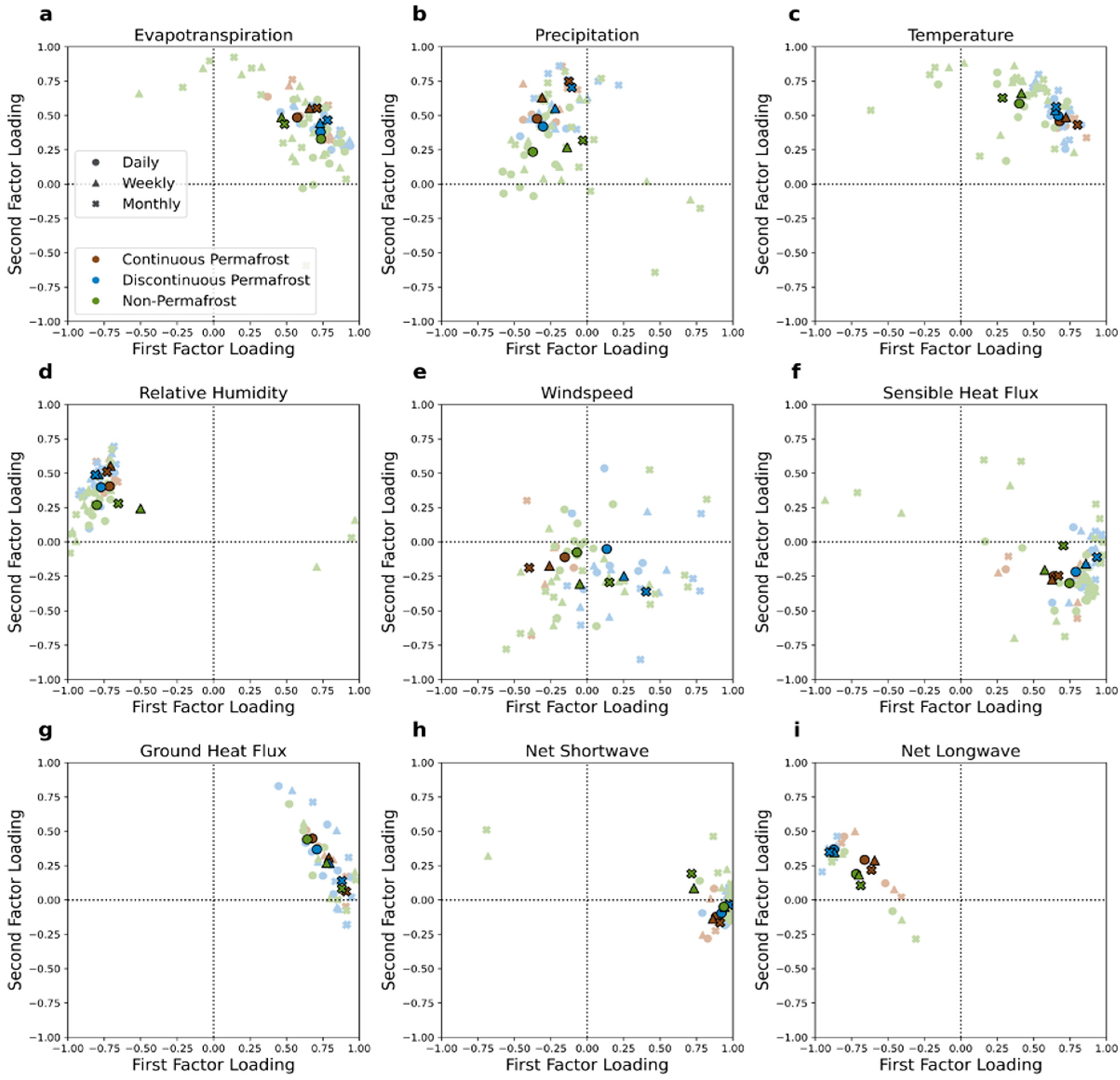
3.1. Factor Analysis

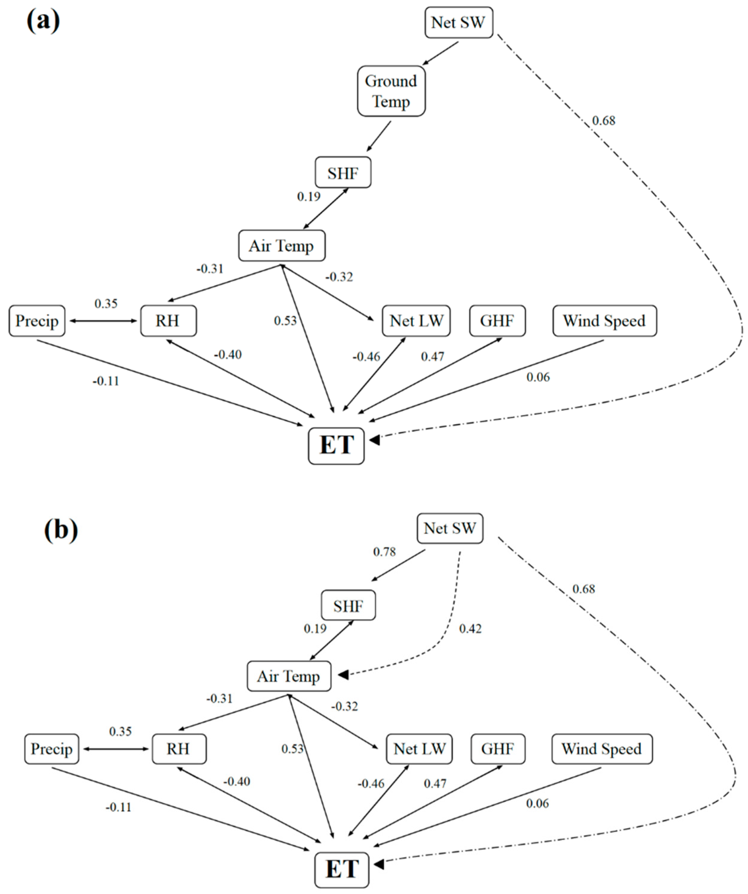
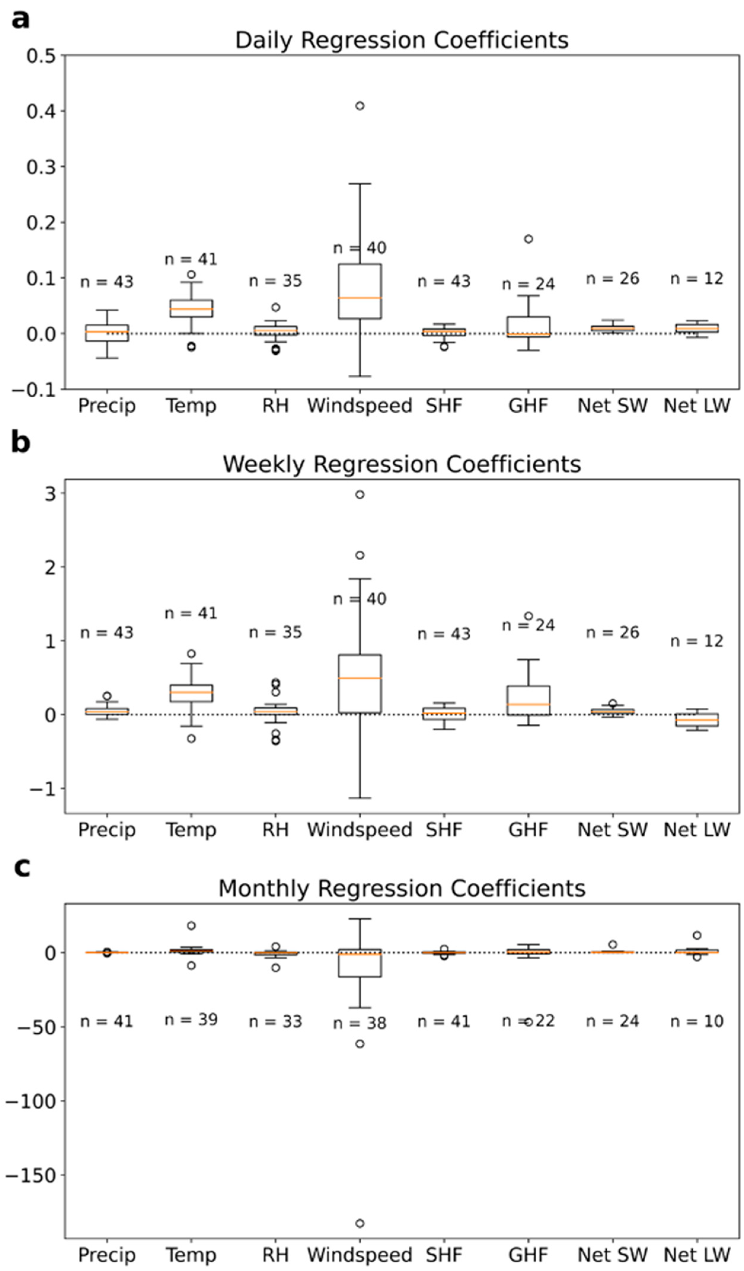
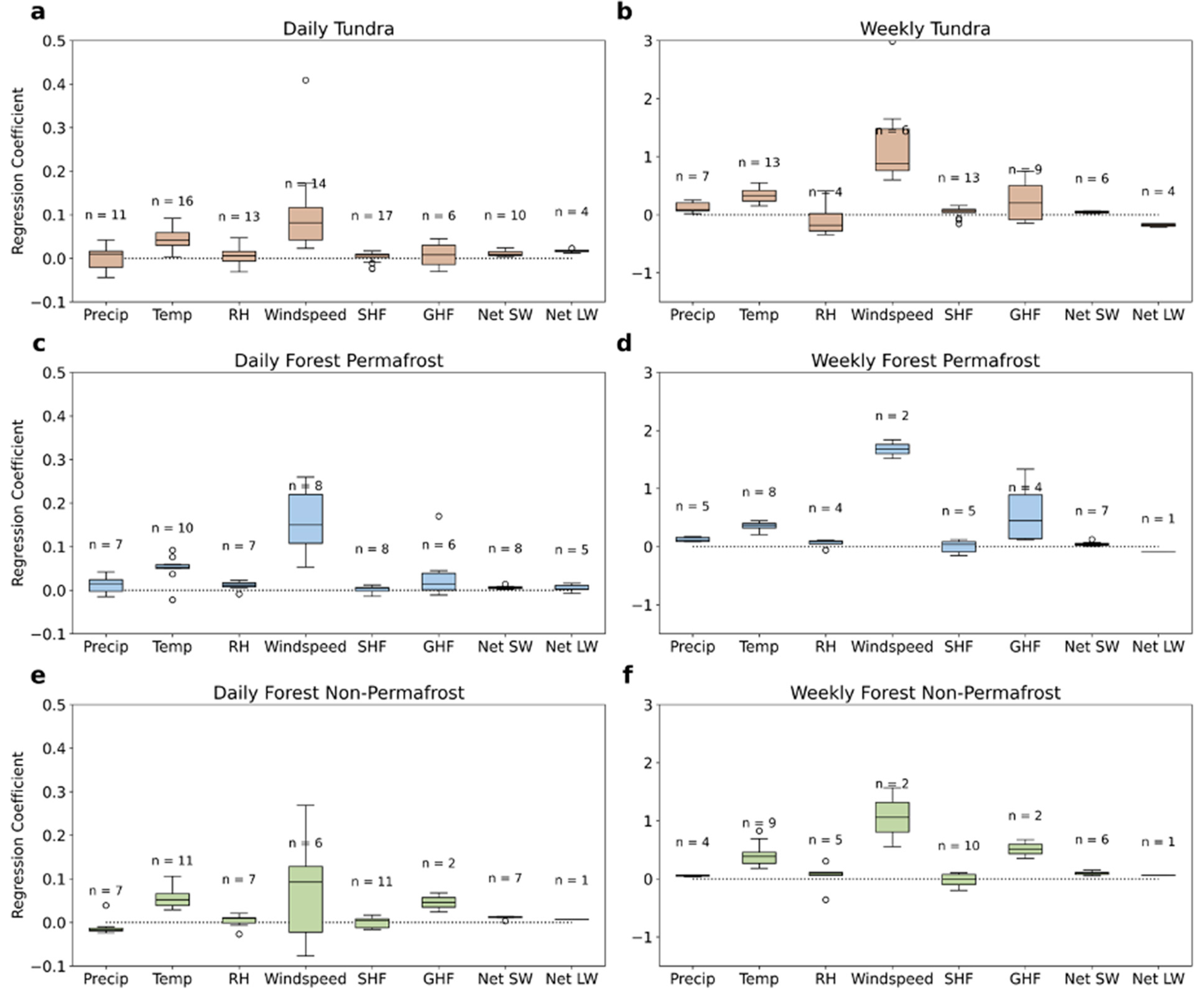
Figure 2 shows the correlation matrix for all sites at the daily, weekly, and monthly scales between all variables as an initial investigation into these relationships. In these correlation plots, ET correlates highly (|r| > 0.5) with net shortwave radiation, ground heat flux, and temperature on the daily, weekly, and monthly scales with sensible heat flux becoming highly correlated at the monthly scale. Precipitation and wind speed have low (|r| < 0.25) correlation with ET on all timescales. Net shortwave radiation has the largest correlation with ET and is also highly correlated with relative humidity, sensible heat flux, ground heat flux, and net longwave radiation on all timescales. Generally, these correlations increase in magnitude as the timescale increases.

As shown in the correlation plots above, many of these variables share similar behaviors and a method is needed to quantify the contribution of each variable to variability patterns. The factor analysis described in Section 2.3 was run across all sites and variables listed in Table 1 and Table 2 to categorize these variables into groups showing similar variability. Figure 3 shows the first factor loadings for tundra, forest, and non-permafrost forest sites. ET, temperature, sensible heat flux, ground heat flux, net shortwave, net longwave, and negative relative humidity all load highly on the first factor. Wind Speed and precipitation have low factor loadings, with the precipitation loadings becoming more positive with increased timescale. The main difference between forest, tundra, is that relative humidity tends to load more strongly negative for forest sites than for tundra. Temperature also loads lower for non-permafrost sites than for permafrost sites.

The factor analysis produces multiple factor loadings with the first factor capturing approximately 50% of the variability in the dataset. Score plots were made to show the loadings on both the first and second factors for all variables. Figure 4 shows score plots grouped by tundra, forest, and non-permafrost forest sites similar to the groupings in Figure 3. All individual sites are shown by the muted markers, categorized by color and time scale (daily, weekly, and monthly), and the average factor loadings for each group are shown by the fully saturated and outlined markers. Figure 4 shows the same results as Figure 3, although the spread among sites is apparent. Precipitation and wind speed have a large spread in both factors with the average second factor loading slightly positive for precipitation. Tundra sites show a more consistent spread in the first factor for the thermal variables ET, temperature, and sensible heat flux.

It is also useful to compare the factor loadings by permafrost presence or absence. Figure 5 and Figure 6 show score plots for tundra and forest, respectively, with sites grouped by permafrost status. Consistent with Figure 4, ET, temperature, sensible heat flux, ground heat flux, net shortwave, net longwave, and negative relative humidity load highly on the first factor for all permafrost groups in both tundra and forest. The low factor loadings for temperature at the non-permafrost forest sites in Figure 3c are supported by a decreasing trend in factor loading as permafrost status decreases in Figure 5 and Figure 6 for both tundra and forest. ET shows a similar relationship to temperature for the tundra sites, but this pattern is not apparent in the forest sites.

The final comparison in this analysis was based on a grouping of the factor loadings by vegetation type for forest and tundra sites. The score plots for tundra and forest sites were grouped by vegetation type: shrubland, wetland, and grassland for tundra, and deciduous needleleaf, wetland, evergreen needleleaf, and deciduous broadleaf for forest sites. Most tundra sites fall under the shrubland and wetland categories, with two sites in the grassland category. The majority of the forest sites were evergreen needleleaf forest, with six sites making up the remaining categories. While the results are not presented graphically here, they can be summarized as follows. For the tundra, the two grassland sites load distinctly lower on the first factor than shrubland and wetland sites for relative humidity. This indicates that for the grassland sites, relative humidity does not follow as similar a pattern to ET as it does at the shrubland and wetland sites. Shrubland sites load slightly lower than other sites for ET, temperature, and sensible heat flux, and load distinctly more positive on wind speed. In general, the forest sites show a larger spread in the first factor for ET, temperature, and sensible heat flux, and a lower spread in relative humidity than the tundra sites. Wind Speed is slightly negative in the second factor loading and precipitation is slightly positive.

3.2. Path Analysis

While a factor analysis quantifies relationships among a complex set of inter-correlated variables, correlations deduced from factor loadings do not provide measures of the relative importance of a variable after removal of the effects of other inter-related variables. Therefore, we supplement the factor analysis with a path analysis to show the direct dependencies of ET on each variable independent of all other variables. Following the approach used by Zhang et al. (2015), the distinction between the direct and indirect dependencies is illustrated in Figure 7, which shows the associations between the different variables in terms of physical pathways. The quantified relationships are based on the daily values (Figure 2a). Consistent with the factor analysis, Figure 7 shows that net solar radiation is the variable most strongly related to ET. However, as shown in the left portion of each diagram, solar radiation drives ET through its effect on temperature via the flux of sensible heat from the ground surface. As parameterized in many models, the sensible heat flux is proportional to the difference between the ground (skin) temperature and the air temperature. Air temperature, in turn, affects ET through its effects on relative humidity and downwelling longwave radiation. ET’s relationships with precipitation and wind speed are weak, although the relationship with wind speed strengthens when the unique contributions of each variable are evaluated as described below.

While Figure 2 shows the actual correlations, the inter-relatedness of the variables implies that these correlations are not measures of the independent contributions of the different variables. We therefore used the path analysis SEM approach, whereby the regression coefficients serve as metrics of independent contributions of the different variables. Figure 8 shows the distribution of regression coefficients for each variable from all runs of the path analysis at the daily, weekly, and monthly scales. Wind speed stands out as having both the largest regression coefficient and largest spread in coefficients. The scale of the regression coefficients increases with increased timescale (note the different y-axis scales in Figure 8), a consequence of the large timescales being sums of the smaller timescale values. The results shown here include extreme outliers in both wind speed and ground heat flux.

Results from the path analysis are subject to error from small sample size and poor model fit. When comparing results of the path analysis across vegetation and permafrost status, only those results with significant p-values were included. Figure 9 shows the combined results of the path analysis for only the sites having p-values significant at the 95% confidence interval; this restriction excludes results with both poor model fit and low sample size. Model runs at the monthly scale were mostly all insignificant with low sample size so only the daily and weekly runs were included for the analysis. Wind speed continues to stand out with the highest median regression coefficient for all sites, with temperature and ground heat flux as the next largest coefficients respectively.

Similar to the factor analysis, the path analysis results were compared by tundra and forest, permafrost, and vegetation differences. Figure 10 shows the distribution of path analysis regression coefficients for tundra, forest, and non-permafrost forest sites for the daily (left) and weekly (right) timescales. Wind speed has the highest regression coefficient in all categories with tundra having the lowest median regression coefficients. The non-permafrost forest sites have a large range of wind speed coefficients on the daily timescale with the lower 1.5 interquartile range dipping slightly negative. On the daily scale, temperature has the second highest regression coefficient for all categories. Both ground heat flux and temperature have relatively high regression coefficients on the weekly scale for forest sites.

Separating the path analysis results by permafrost status shows several key differences in permafrost status consistent between forest and tundra sites. Figure 11 and Figure 12 show the path analysis regression coefficients for tundra and forest sites, respectively, separated into continuous, discontinuous, and non-permafrost sites. Wind speed had the largest regression coefficient for all permafrost types in both the forest and tundra with distinctly higher coefficients for discontinuous permafrost sites. Non-permafrost forest sites have the largest range of wind speed regression coefficients with both positive and negative values. Temperature has the second highest coefficient. However, ground heat flux has a similar regression coefficient for the forest non-permafrost sites. The continuous permafrost in both the forest and tundra show the smallest differences in regression coefficients between variables.

Tundra and forest sites were separated by vegetation types for the final comparisons of path analysis results. Because the results for the different vegetation types generally showed smaller differences than for the permafrost states, we present only the following summary. In the tundra shrubland and wetland sites wind speed continues to stand out with the highest regression coefficient. However, this relationship does not appear in the grassland sites. There is no variable with a significantly larger regression coefficient than others for the grassland sites. In both tundra shrubland and wetland sites, temperature has the second highest regression coefficient for all timescales. Ground heat flux has the largest range of regression coefficients for shrubland sites at the weekly timescale. Most forest sites fall under the evergreen needleleaf vegetation, showing wind speed with the highest regression coefficient and largest range. Temperature is the second highest regression coefficient. However, ground heat flux becomes similar to temperature in the magnitude of its regression coefficient. Although the sample size is low for the other forest vegetation types, wind speed continues to have the highest regression coefficient with the highest coefficients at the wetland sites.

To test the significance of differences in the regression coefficients of different variables in the path analysis, a Kruskal–Wallis test was run for all categories in the present section over all variables. Results from the Kruskal–Wallis tests are shown in

Table 3. Kruskal–Wallis test statistic (H-value) and p-values for all path analysis categories. All variable regression coefficients are included as the test distributions. Non-significant p-values (p > 0.05) are shaded in gray.

	Test Statistic		p-Value
	Daily	Weekly	Daily	Weekly
Tundra Permafrost Continuous	29.59	26.12	0	0
Tundra Permafrost Discontinuous	12.27	10.78	0.09	0.15
Tundra Non-Permafrost	12.96	3.2	0.07	0.87
Forest Permafrost Continuous	12.36	8.87	0.09	0.26
Forest Permafrost Discontinuous	22.02	19.35	0	0.01
Forest Non-Permafrost	26.65	28.14	0	0
Tundra Wetland	26.98	23.24	0	0
Tundra Shrubland	23.77	18.3	0	0.01
Tundra Grassland	5.93	3.2	0.55	0.87
Forest Evergreen Needleleaf	30.48	37.72	0	0
Forest Deciduous Needleleaf	4	3	0.78	0.89
Forest Deciduous Broadleaf	11.36	5.92	0.12	0.55
Forest Wetland	9.04	7.68	0.25	0.36
Tundra	50.42	39.29	0	0
Forest Permafrost	32.01	27.26	0	0
Forest Non-Permafrost	26.65	28.14	0	0
All Sites	98.21	87.2	0	0

,

Table 4. Kruskal–Wallis test statistic (H-value) and p-values for all path analysis categories. Temperature, ground heat flux, and windspeed regression coefficients are included as the test distributions. Non-significant p-values (p > 0.05) are shaded in gray.

	Test Statistic		p-Value
	Daily	Weekly	Daily	Weekly
Tundra Permafrost Continuous	5.99	10.48	0.05	0.01
Tundra Permafrost Discontinuous	5.38	3.2	0.07	0.2
Tundra Non-Permafrost	3	0	0.22	1
Forest Permafrost Continuous	3.2	1.8	0.2	0.41
Forest Permafrost Discontinuous	8.77	4.73	0.01	0.09
Forest Non-Permafrost	0.69	2.74	0.71	0.25
Tundra Wetland	10.85	10.5	0	0.01
Tundra Shrubland	4.11	2.54	0.13	0.28
Tundra Grassland	0	0	1	0
Forest Evergreen Needleleaf	3.07	3.47	0.22	0.18
Forest Deciduous Needleleaf	1	0	0.61	0
Forest Deciduous Broadleaf	4.29	0	0.12	1
Forest Wetland	3.6	2.4	0.17	0.3
Tundra	11.75	13.14	0	0
Forest Permafrost	11.95	4.8	0	0.09
Forest Non-Permafrost	0.69	2.74	0.71	0.25
All Sites	20.73	20.29	0	0

and

Table 5. Kruskal–Wallis test statistic (H-value) and p-values for all path analysis categories. Temperature and ground heat flux regression coefficients are included as the test distributions. Non-significant p-values (p > 0.05) are shaded in gray.

	Test Statistic		p-Value
	Daily	Weekly	Daily	Weekly
Tundra Permafrost Continuous	3.46	0.66	0.06	0.42
Tundra Permafrost Discontinuous	1.93	1.8	0.16	0.18
Tundra Non-Permafrost	0	0	1	1
Forest Permafrost Continuous	1.8	1.8	0.18	0.18
Forest Permafrost Discontinuous	1.12	0.56	0.29	0.46
Forest Non-Permafrost	0.35	0.22	0.55	0.64
Tundra Wetland	4.19	2.45	0.04	0.12
Tundra Shrubland	1.36	0	0.24	1
Tundra Grassland	0	0	1	0
Forest Evergreen Needleleaf	1.19	0	0.28	1
Forest Deciduous Needleleaf	0	0	0	0
Forest Deciduous Broadleaf	1.8	0	0.18	1
Forest Wetland	1.5	0	0.22	1
Tundra	4.59	0.59	0.03	0.44
Forest Permafrost	2.31	0	0.13	1
Forest Non-Permafrost	0.35	0.22	0.55	0.64
All Sites	7.77	0.26	0.01	0.61

. All sites showed significant (p ≤ 0.05) differences between variables for both daily and weekly timescales. The categories that showed significant differences in regression coefficients on all timescales for all variables are tundra, forest permafrost, forest non-permafrost, forest evergreen needleleaf, tundra shrubland, tundra wetland, forest discontinuous permafrost, and tundra continuous permafrost. In comparison, the tundra discontinuous and non-permafrost, forest continuous permafrost, tundra grassland, forest wetland, forest deciduous needleleaf, and forest deciduous broadleaf categories showed no significant differences between variables on all timescales. The Kruskal–Wallis test does not give information on which variables show significant differences, so the test was performed twice more including only the temperature and ground heat flux variables, with a final test also including wind speed. Only the daily runs of all sites, tundra, and tundra wetland showed significant differences between temperature and ground heat flux. When wind speed was included, significant differences were found for the previous categories as well as tundra continuous permafrost, forest discontinuous permafrost, and forest permafrost. This indicates that wind speed is a significant contributor to ET variability. We conclude that, for the sites where significant differences were found when wind speed was added, wind speed makes a significant independent contribution to ET variability.

Throughout the path analysis, wind speed had the largest regression coefficient onto ET, while the factor analysis found wind speed to have low loadings onto the first factor, which explained approximately 50% of the variability in ET. To quantify the extent of influence wind speed has on ET, multiple regressions were run for the same sites and variables as the path analysis. The explained variance was evaluated from multiple regressions with and without wind speed, as well as the percentage of contribution from wind speed to the total variability. This was calculated as the difference in the two explained variances divided by the total variance. The average total variance in ET on the daily timescale is 0.58 with a standard deviation of 0.21. The contribution from wind speed is 1.19% with a standard deviation of 1.94%. At the weekly scale, the average total variance is 19.0 with a standard deviation of 6.75, and the average contribution from wind speed is 0.71% with a standard deviation of 0.92%. Therefore, the actual contributions from wind speed to the total variance are low even though wind speed appears to have the largest independent influence on ET in the path analysis.

4. Discussion

4.1. Factor Analysis

Among the multiple structural equation models, the factor analysis was performed to identify groups of variables with shared variability patterns with ET. For both tundra and boreal sites, ET had high positive correlations with net shortwave radiation, temperature, ground heat flux, and sensible heat flux. These variables all display a strong seasonal cycle increasing in magnitude over the warm season, peaking around July. Net shortwave radiation is the primary driver of these seasonal cycles with the strong correlations shown in Figure 2. Within the connected seasonal cycles, the high sensible heat flux loadings are consistent with an excess of available surface energy during episodes of increased ET. Moreover, the strong negative correlation between ET and relative humidity and strong positive correlation with temperature is consistent with the findings of [7,10] that warm and dry conditions are associated with enhanced ET. Interestingly, these thermal drivers dominate the daily variations of ET as wind speed and precipitation show low correlations.

In the factor analysis, solar radiation is implicated as a key driver of ET through its high factor loading on the first factor, explaining most of the variance of ET. Solar radiation is also a major driver of temperature and contributes to variations in downwelling longwave radiation, impacting the surface temperature. Additionally, incoming net radiation is linked to ground temperature in part through high loadings of the surface–atmosphere sensible heat flux at both tundra and boreal sites. The longwave component of net radiation is directly influenced by temperature where the solar component does not have this direct link. Variations in solar radiation at the ground surface are strongly dependent on cloudiness, which is positively correlated with precipitation. With reduced cloudiness, drying can be favored through (a) an increase in net surface radiation, temperature and ET and (b) a reduction in P, provided that there is available water at the surface.

An interesting distinction between the boreal and tundra sites is the difference in factor loadings for relative humidity. Relative humidity is one of the highest loading factors at boreal sites with a lower loading at tundra sites. This negative loading, combined with the positive loading of ET in Figure 3 indicates that as relative humidity decreases, ET increases. This is consistent with the bulk transfer formulations used in many climate models (e.g., [9]). The relationship between ET and relative humidity is an active area of research, as several previous studies have found strong correlations between ET and vapor pressure deficit (VPD) for boreal forest ecosystems [15,16,17,18]. The ET–VPD correlations found in those studies are consistent with the high loading of relative humidity in Figure 3.

The large control of solar radiation on ET and other associated drivers, as well as the differences in relative humidity loadings between tundra and boreal sites indicate that tundra sites are more temperature limited than moisture limited. The strong loadings of temperature and solar radiation in Figure 3 for tundra sites reinforces the importance of temperature. Interestingly, precipitation loads slightly negative for daily runs and slightly positive for monthly runs. This points to a possible linkage to photosynthetic activity (transpiration) over several weeks following a precipitation event. The negative loadings for the daily runs imply that precipitation does not have an immediate impact on evaporation and ET in general. The implication is that the system is not limited by the available water, i.e., ET is limited by the available energy so that even when there is plenty of water, ET depends on the surface energy balance (or imbalance). Additionally, the correlations shown in Figure 2 show that precipitation has minor importance as a driver of ET. While this conclusion applies to the high-latitude sites in the present study, precipitation is clearly relevant as a water source in lower-latitude locations such as mid-latitude deserts.

The role of temperature on the overall variability of ET appears to have a relationship with permafrost. In both tundra and forest sites, temperature loads higher on the first factor with higher amounts of permafrost, one of the most distinguishing differences between the two ecosystems. [11] describes permafrost acting as a buffer in the energy partitioning into sensible and ground heat fluxes to influence surface air temperatures. This buffer can impact the responses of thermal variables such as temperature to increased solar radiation during the warm season. Although the reasoning is not apparent, this mechanism appears to act opposite in the factor analysis used in this study. In areas with more permafrost, the variability in air temperature follows similar patterns to increased net solar radiation than in areas with less permafrost. This behavior is also seen in ET at tundra sites, with ET following more similar variability patterns as radiation and thermal variables for areas with more permafrost than those without. Some of this variability may also be due to the overall heterogeneity in tundra vegetation, coupled with microtopographic differences in air temperature and soil temperature, that influence vegetation composition (including differences in mosses, lichens, grasses, forbs, and sedges) and thus ET [30]. Understanding how these relationships connect and affect ET variability is a crucial area for future research to accurately model and predict future soil moisture in the Arctic.

4.2. Path Analysis

While wind speed was not among the variables with similar variability patterns to ET in the factor analysis, it overwhelmingly shows the most influence on ET, independent from other variables in the path analysis. In all comparisons of the path analysis results, wind speed stood out with both the largest regression coefficients on ET and the largest range in coefficients. Wind speed was not among the group of variables with high factor loadings in the factor analysis and does not follow a distinct seasonal cycle over the warm season in response to increased solar radiation. Together, these results can be interpreted to conclude that wind speed has the largest independent influence on ET. These effects are more pronounced at boreal forest sites than tundra, with non-permafrost forest sites showing the largest variability. However, discontinuous permafrost sites in both boreal forest and tundra show the largest effects of wind speed on ET. Although sample size is low (2) for wetland forest sites underlain by discontinuous or an absence of permafrost, wind speed stands distinctly above all other variables. The relative importance of wind speed is likely related to its role in turbulent mixing. For example, strong winds in the afternoon have recently been shown to enhance mechanical turbulence and increase evaporation over a lake in the Atacama Desert of Chile [31].

This overwhelming dependency on wind speed is unique. The authors of [8] evaluated atmospheric controls on ET at a station in north China using a path analysis. Net radiation, air temperature, vapor pressure deficit, and wind speed were used to predict ET with specified covariances between every predictor variable. Wind speed was found to have the least both direct and indirect effect on ET with net radiation having the largest direct effect. The stations used in the present analysis are remote, high-latitude, and many are underlain by permafrost, while [8] examined a mid-latitude agricultural irrigated site.

Permafrost has a distinct effect on the differences between variables in the path analysis. In both boreal forest and tundra, continuous permafrost sites show small differences in regression coefficients between variables, while discontinuous and non-permafrost sites show more pronounced differences. The presence of permafrost has a damping effect on independent variable contributions to ET variability. Although the tundra lacks even coverage of non-permafrost sites and the boreal forest lacks continuous permafrost sites, the damping effect is seen in both boreal and tundra ecosystems.

Second to wind speed, temperature and ground heat flux show the greatest effects on ET. Unlike wind speed, the temperature regression coefficients are relatively consistent between vegetation types, permafrost status, and timescale aside from the natural increase in coefficients as the timescale increases. This implies the individual effects of temperature are consistent across vegetation and permafrost and show little variability. Compared to the differences in the factor analysis temperature loadings by permafrost, the consistency seen in the path analysis further implies that the different factor loadings on temperature arise from associations with other variables such as solar radiation. Ground heat flux does not show this consistency: as the timescale increases, ground heat flux increases in relative importance at forest sites. On the weekly timescale ground heat flux becomes comparable to temperature in its regression coefficients. As described in [32], ground heat flux has large diurnal variability, contributing to lower regression coefficients on the daily scale. This variability is smoothed by the longer timescales and the regression coefficient onto ET increases in response.

5. Conclusions

Based on the preceding discussion, the following are the main conclusions of this study:

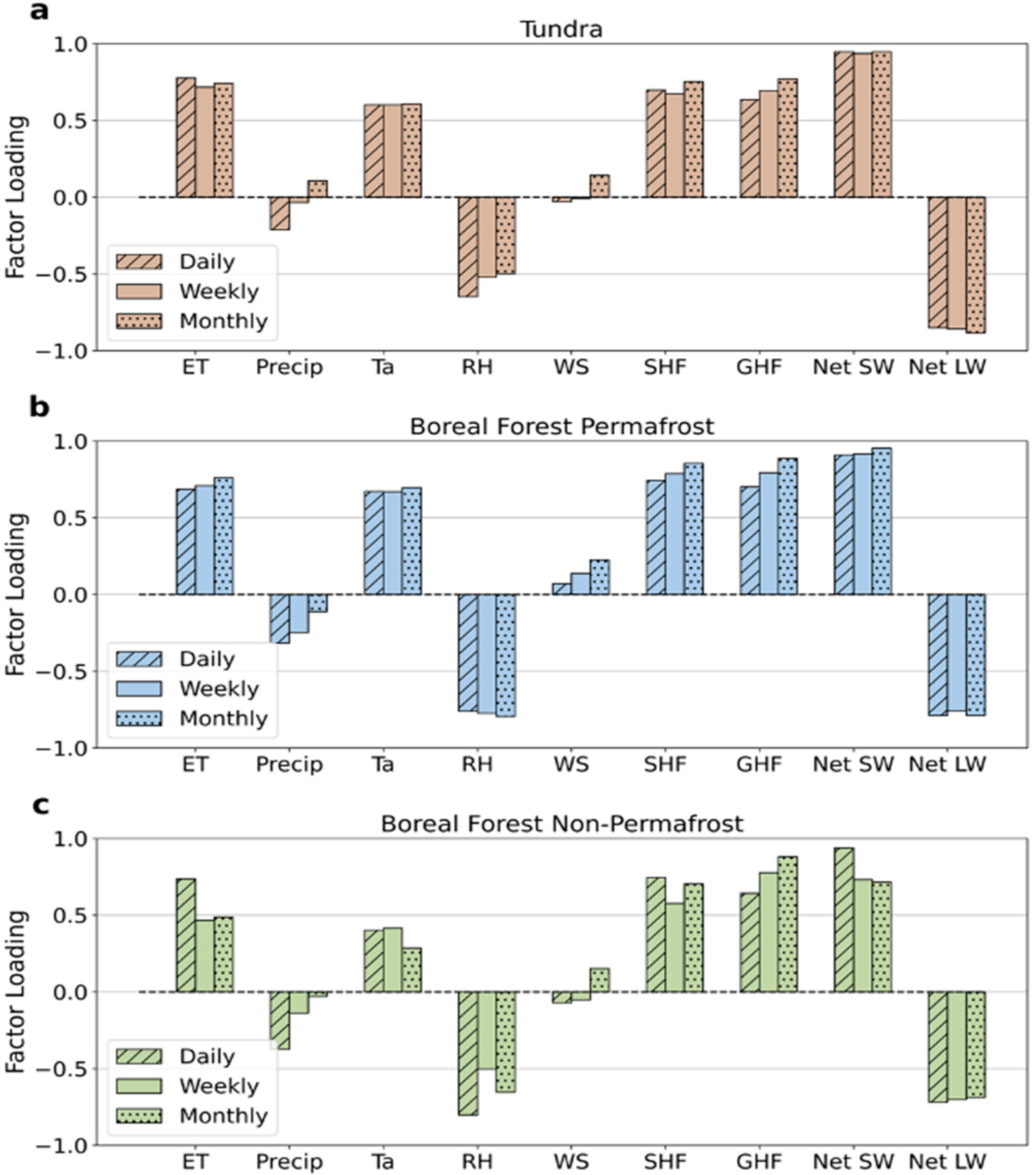
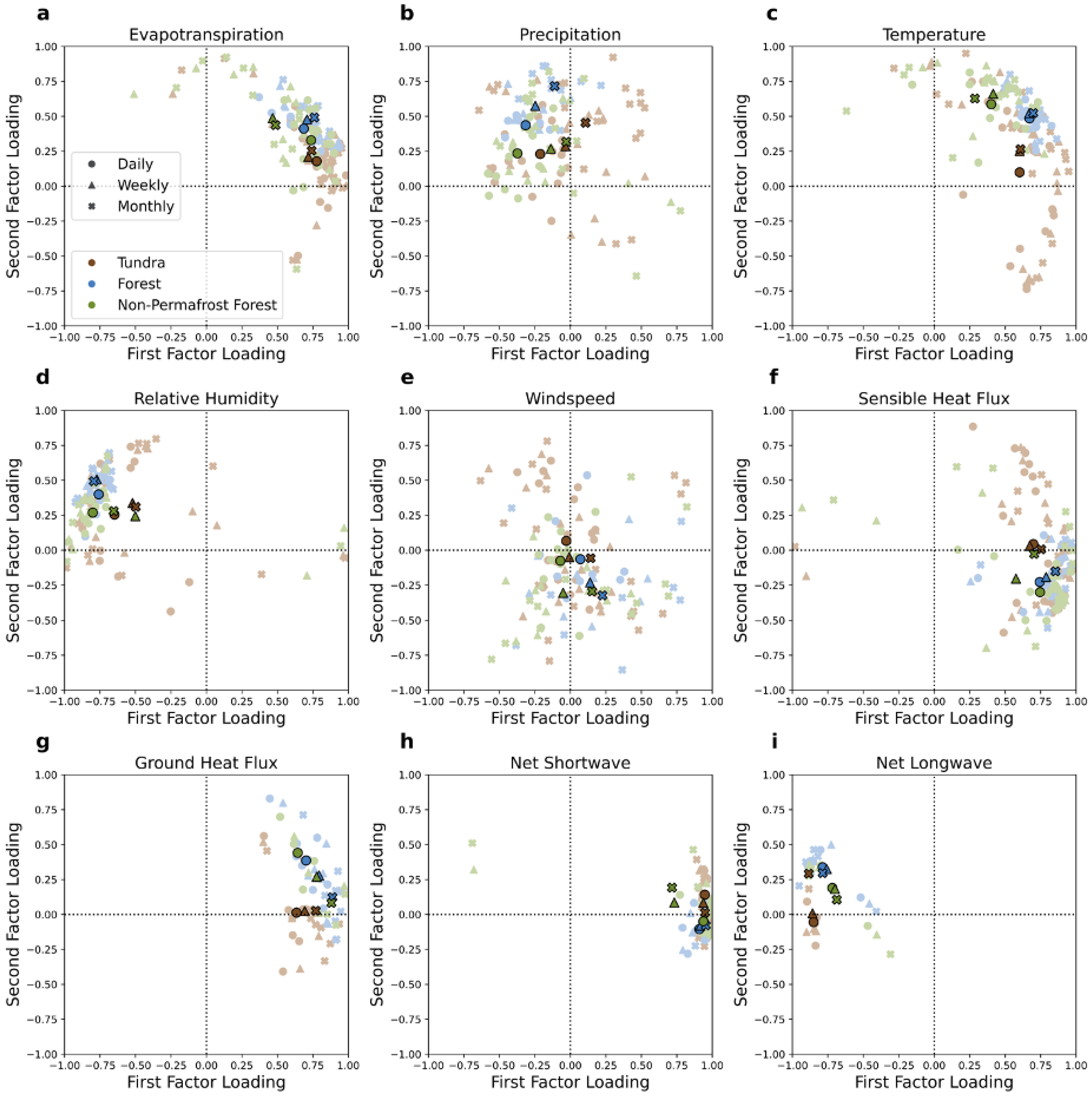
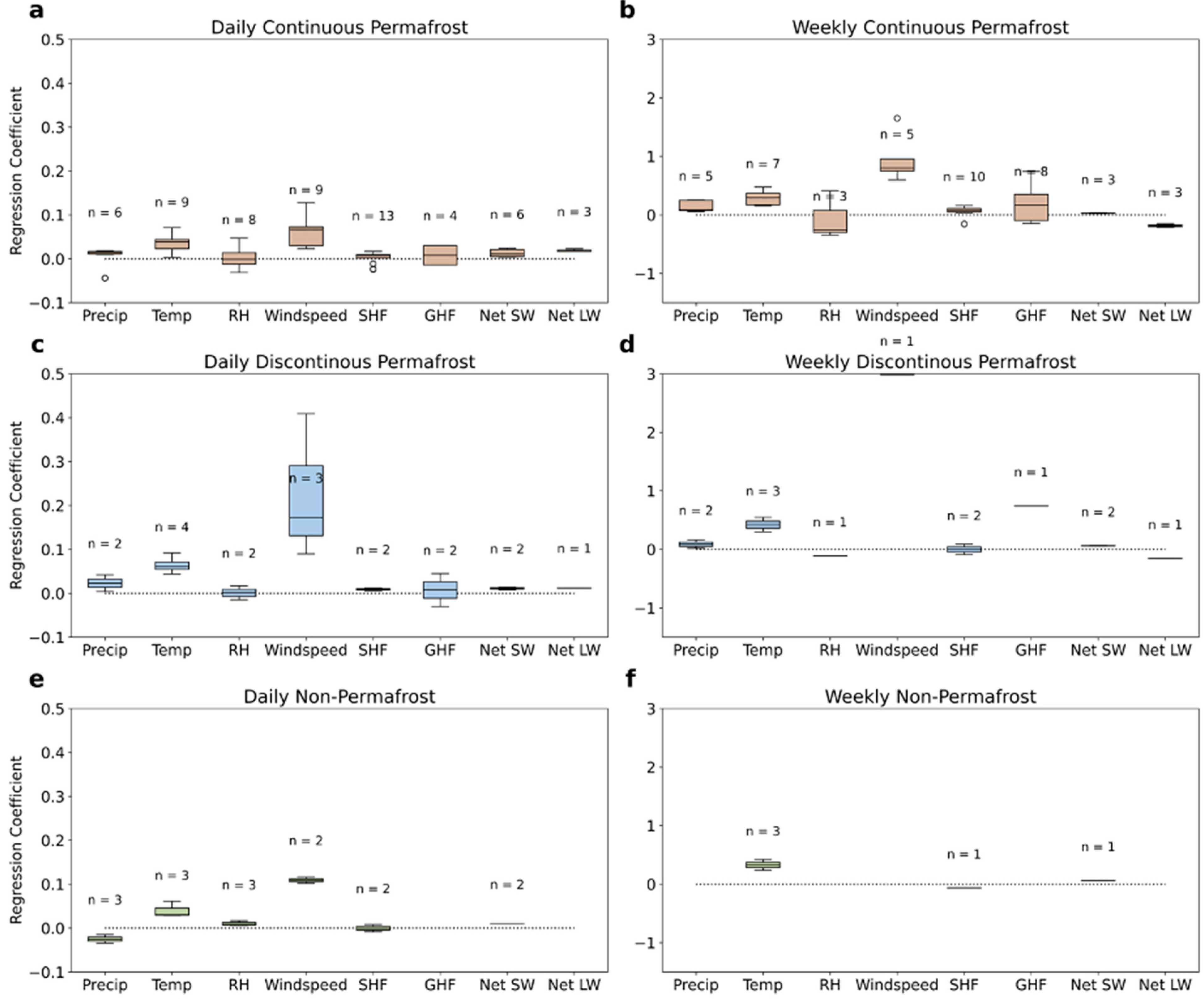
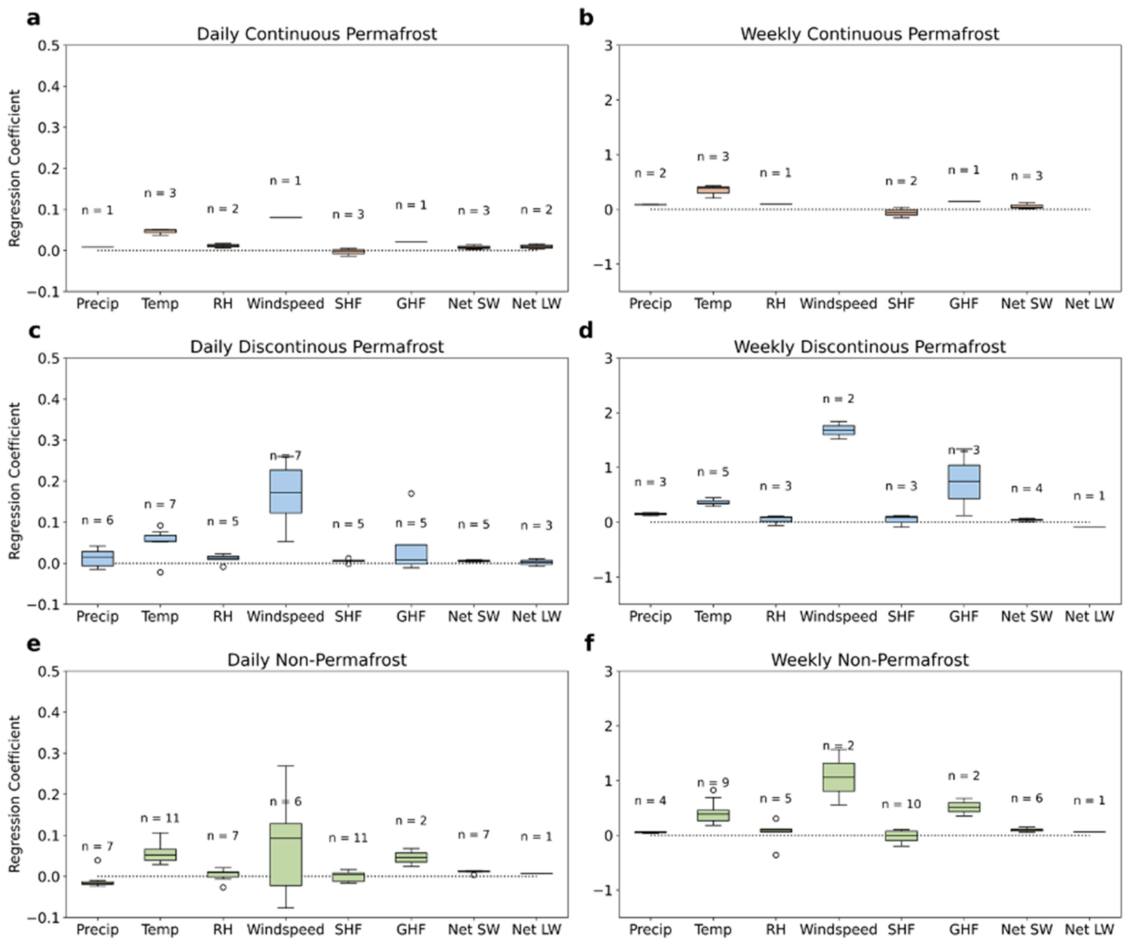
• Overall variability in ET at forest sites shows a stronger dependence on relative humidity while ET at tundra sites depends more strongly on air temperature and thermal variables. The results imply that ET at tundra sites is more temperature-limited than moisture-limited.
• The flow chart accompanying the path analysis shows that ET has a stronger direct correlation with solar radiation than with any other measured variable.
• Wind speed has the largest independent contribution to ET variability. The independent contribution of solar radiation is smaller because solar radiation also affects ET through the air temperature, which in turn is correlated with relative humidity and net longwave radiation. The independent contribution of wind speed is especially apparent at forest wetland sites, although the sample size of these sites is small.
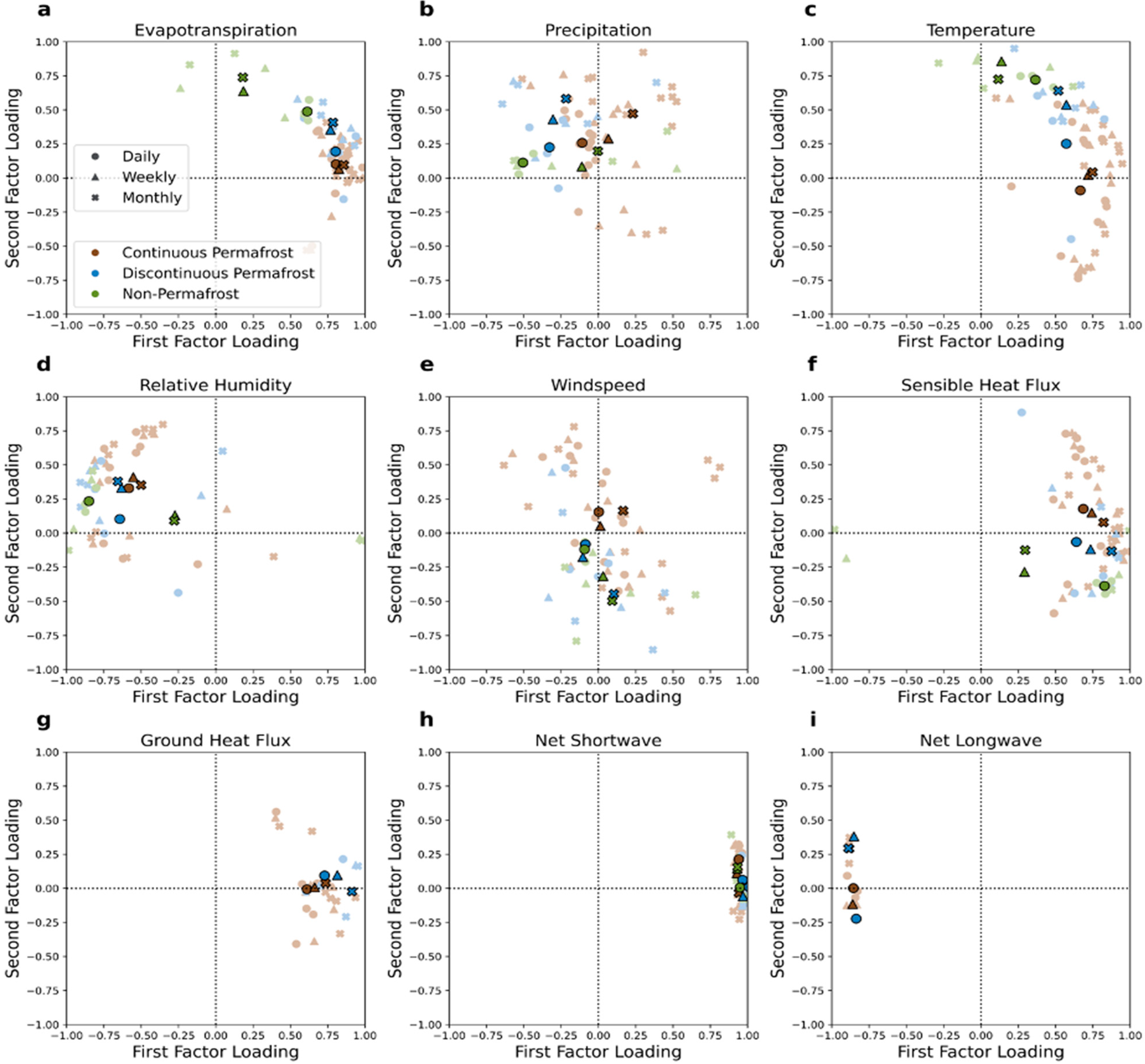
• The role of temperature in the overall variability of ET appears to be permafrost-dependent. For both tundra and forest sites, temperature loads higher on the first factor when permafrost is present, a result that is common to both types of vegetation. More generally, the presence of permafrost has a damping effect on independent variable contributions to ET variability.

The last of these conclusions has implications for the trajectory of cold-region ET in a warming climate. Permafrost thaw driven by increasing air temperatures will reduce the extent of frozen ground. As larger areas become permafrost-free, temperature’s role as a driver will diminish in comparison with other variables, potentially increasing the influence of variables such as relative humidity and wind speed on ET variations over daily to monthly timescales. More specifically, the ET may become less temperature-limited and more moisture-limited in high-latitude terrestrial regions. The ability of models to capture the dependence on moisture availability would then be increasingly important for the validity of their simulation of changes in the moisture budget of northern regions. The results presented here can provide a basis for assessing the validity of model simulations of variations in ET, although one must reckon with the challenges of scale discrepancies: the data used in this study are essentially point measurements, while climate models have resolutions ranging from several kilometers to hundreds of kilometers.

References

1. Mackay, D.S.; Ewers, B.E.; Cook, B.E.; Davis, K.J. Environmental drivers of evapotranspiration in a shrub wetland and an upland forest in northern Wisconsin. Water Resour. Res. 2007, 43, W03442. [Google Scholar] [CrossRef] [Green Version]
2. Zhang, Y.; Ma, N.; Park, H.; Walsh, J.E.; Zhang, K. Evaporation processes and changes over the northern regions. In Arctic Hydrology, Permafrost and Ecosystems; Yang, D., Kane, D.L., Eds.; Springer: Cham, Switzerland, 2021; pp. 101–131. [Google Scholar] [CrossRef]
3. Bring, A.; Federova, I.; Dibike, Y.; Hinzman, L.; Mard, J.; Mernild, S.H.; Prowse, T.; Semenova, O.; Stuefer, S.L.; Woo, M.-K. Arctic terrestrial hydrology: A synthesis of processes, regional effects, and research challenges. J. Geophys. Res. Biogeosci. 2016, 121, 621–649. [Google Scholar] [CrossRef]
4. Hiyama, T.; Yang, D.; Kane, D. Permafrost hydrology: Linkages and feedbacks. In Arctic Hydrology, Permafrost and Ecosystems; Yang, D., Kane, D.L., Eds.; Springer: Cham, Switzerland, 2021; pp. 471–491. [Google Scholar] [CrossRef]
5. Smith, S.L.; Romanovsky, V.E.; Lewkowicz, A.G.; Burn, C.R.; Allard, M.; Clow, G.D.; Yoshikawa, K.; Throop, J. Thermal state of permafrost in North America: A contribution to the international polar year. Permafr. Periglac. Process. 2010, 21, 117–135. [Google Scholar] [CrossRef] [Green Version]
6. Brown, R.; Marsh, P.; Dery, S.; Yang, D. Snow cover—Observations, processes, changes and impacts. In Arctic Hydrology, Permafrost and Ecosystems; Yang, D., Kane, D.L., Eds.; Springer: Cham, Switzerland, 2021; pp. 61–99. [Google Scholar] [CrossRef]
7. Liljedahl, A.K.; Hinzman, L.D.; Harazono, Y.; Zona, D.; Tweedie, C.E.; Hollister, R.D.; Engstrom, R.; Oechel, W.C. Nonlinear controls on evapotranspiration in arctic coastal wetlands. Biogeosciences 2011, 8, 3375–3389. [Google Scholar] [CrossRef] [Green Version]
8. Zhang, B.; Xu, D.; Liu, Y.; Li, F.; Cai, L.; Du, L. Multi-scale evapotranspiration of summer maize and the controlling meteorological factors in North China. Agric. For. Meteorol. 2015, 216, 1–12. [Google Scholar] [CrossRef]
9. Trenberth, K.E. Climate System Modeling; Cambridge University Press: Cambridge, UK, 2010; p. 820. ISBN -13: 978-0521128377. [Google Scholar]
10. Nazarbakhsh, M.; Ireson, A.M.; Barr, A.G. Controls on evapotranspiration from Jack Pine Forests in the Boreal Plains Ecozone. Hydrol. Process. 2019, 34, 927–940. [Google Scholar] [CrossRef]
11. Eugster, W.; Rouse, W.R.; Pielke, R.A., Sr.; McFadden, J.P.; Baldocci, D.D.; Kittell, T.G.F.; Chapin, F.S.; Liston, G.E.; Vidale, P.L.; Vaganov, E.; et al. Land-atmosphere energy exchange in Arctic Tundra and Boreal Forest: Available data and feedbacks to climate. Glob. Chang. Biol. 2002, 6, 84–115. [Google Scholar] [CrossRef]
12. Sabater, A.M.; Ward, H.C.; Hill, T.C.; Gormall, J.L.; Wade, T.J.; Evans, J.G.; Preto-Blanco, A.; Disney, M.; Phoenix, G.K.; Williams, M.; et al. Transpiration from subarctic deciduous woodlands: Environmental controls and contribution to ecosystem evapotranspiration. Ecohydrology 2019, 13, e2190. [Google Scholar] [CrossRef]
13. Dolman, A.J.; Maximov, T.C.; Moors, E.J.; Maximov, A.P.; Elbers, J.A.; Koronov, A.V.; Waterloo, M.J.; van der Molen, M.K. Net ecosystem exchange of carbon dioxide and water of far eastern Siberian Larch (Larix cajanderii) on permafrost. Biogeosciences 2004, 1, 133–146. [Google Scholar] [CrossRef] [Green Version]
14. Kosugi, Y.; Takanashi, S.; Tanaka, H.; Ohkubo, S.; Tani, M.; Yana, K.; Katayama, T. Evapotranspiration over a Japanese cypress forest. I: Eddy covariance fluxes and surface conductance characteristics for 3 years. J. Hydrol. 2007, 337, 269–283. [Google Scholar] [CrossRef]
15. Ohta, T.; Maximov, T.C.; Dolman, A.J.; Nakai, T.; van der Molen, M.K.; Kononov, A.V.; Maximov, A.P.; Hiyama, T.; Iijima, Y.; Moors, E.J.; et al. Interannual variation of water balance and summer evapotranspiration in an eastern Siberian larch forest over a 7-year period (1998–2006). Agric. For. Meteorol. 2008, 148, 1941–1953. [Google Scholar] [CrossRef]
16. Brümmer, C.; Black, A.T.; Jassal, R.S.; Grant, N.J.; Spittlehouse, D.L.; Chen, B.; Nesic, Z.; Amiro, B.D.; Arian, M.A.; Barr, A.G.; et al. How climate and vegetation type influence evapotranspiration and water use efficiency in Canadian forest, peatland and grassland ecosystems. Agric. For. Meteorol. 2012, 153, 14–30. [Google Scholar] [CrossRef]
17. Yan, H.; Shugart, H.H. An air relative-humidity-based evapotranspiration model from eddy covariance data. J. Geophys. Res. 2010, 115, D16106. [Google Scholar] [CrossRef] [Green Version]
18. Thunberg, S.M.; Walsh, J.E.; Euskirchen, E.S.; Redilla, K.; Rocha, A.V. Surface moisture budget of tundra and boreal ecosystems in Alaska: Variations and drivers. Polar Sci. 2021, 100685. [Google Scholar] [CrossRef]
19. Saito, K.; Walsh, J.E.; Bring, A.; Brown, R.; Shiklomanov, A.; Yang, D. Future trajectory of Arctic system evolution. In Arctic Hydrology, Permafrost and Ecosystems; Yang, D., Kane, D.L., Eds.; Springer: Cham, Switzerland, 2021; pp. 893–914. [Google Scholar] [CrossRef]
20. Lafleur, P.M.; Humphreys, E.R.; St. Louis, V.L.; Myklebust, M.C.; Papakryiakou, T.; Poissant, L.; Barker, J.D.; Pilote, M.; Swystun, K.A. Variation in peak growing season net ecosystem production across the Canadian Arctic. Environ. Sci. Technol. 2012, 46, 7971–7977. [Google Scholar] [CrossRef]
21. Allen, R.; Pereira, L.; Raes, D.; Smith, M. Crop Evapotranspiration-Guidelines for Computing Crop Water Requirements—FAO Irrigation and Drainage Paper No. 56; United Nations Food and Agriculture Organization (FAO): Rome, Italy, 1998; Volume 56, pp. 26–40. Available online: https://www.scirp.org/reference/referencespapers.aspx?referenceid=1665171 (accessed on 9 October 2021).
22. Mosre, J.; Suárez, F. Actual evapotranspiration estimates in arid cold regions using machine learning algorithms with in situ and remote sensing data. Water 2021, 13, 870. [Google Scholar] [CrossRef]
23. Bollen, K. Structural Equations with Latent Variables; John Wiley and Sons: New York, NY, USA, 1989; p. 709. ISBN 978-0-471-01171-2. [Google Scholar]
24. Gorsuch, R.L. Factor Analysis, 2nd ed.; Routledge Press: London, UK, 2014; p. 464. ISBN 9781138831995. [Google Scholar]
25. UCLA. Statistical Consulting Group. Available online: https://stats.idre.ucla.edu/r/seminars/rcfa/#s2 (accessed on 2 October 2021).
26. Python3 Factor Analyzer Package. Available online: https://libraries.io/pypi/factor-analyzer (accessed on 2 October 2021).
27. Loehlin, J.C. Latent Variable Models: An Introduction to Factor, Path and Structural Analysis, 4th ed.; Lawrence Erlbaum Associates: Mathway, NH, USA, 2003; p. 336. [Google Scholar] [CrossRef]
28. Rosseel, Y. lavaan: An R package for structural equation modeling. J. Stat. Softw. 2012, 18, 1–36. Available online: file:///C:/Users/jewalsh/AppData/Local/Temp/v48i02-1.pdf (accessed on 9 October 2021).
29. Kruskal, W.J.; Wallis, W.A. Use of ranks in one-criterion variance analysis. J. Am. Stat. Assoc. 1952, 47, 583–621. [Google Scholar] [CrossRef]
30. Raz-Yaseef, N.; Young-Robertson, J.; Rahm, T.; Sloan, V.; Newman, B.; Wilson, C.; Wullschleger, S.D.; Torn, M.S. Evapotranspiration across plant types and geomorphological units in polygonal Arctic tundra. J. Hydrol. 2017, 533, 816–825. [Google Scholar] [CrossRef] [Green Version]
31. Lobos-Roco, F.; Hartogensis, O.; Vila-Guerau de Arellano, J.; de la Fuente, A.; Muñoz, R.; Rutllant, J.; Suárez, F. Local evaporation controlled by regional atmospheric circulation in the Altiplano of the Atacama Desert. Atmosphere 2021, 21, 9125–9150. [Google Scholar] [CrossRef]
32. Purdy, A.J.; Fisher, J.B.; Goulden, M.L.; Famiglietti, J.S. Ground heat flux: An analytical review of 6 models evaluated at 88 sites and globally. J. Geophys. Res. Biogeosci. 2016, 121, 3045–3059. [Google Scholar] [CrossRef]
Figure 1. Map of Arctic and subarctic measurement sites used in this study.
Atmosphere 12 01359 g001
Figure 2. Correlation matrices between all variables from all sites at the (a) daily, (b) weekly, and (c) monthly scales.
Atmosphere 12 01359 g002
Figure 3. Loadings of variables in the first pattern of the factor analysis for (a) tundra (b) forest permafrost, and (c) forest non-permafrost sites.
Atmosphere 12 01359 g003
Figure 4. Score plots of the first and second factor loadings for each variable at the daily, weekly, and monthly timescales. Sites are categorized by tundra (brown), boreal forest with permafrost (blue), and boreal forest without permafrost (green). The variables include evapotranspiration (a), precipitation (b), temperature (c), relative humidity (d), wind speed (e), sensible heat flux (f), ground heat flux (g), net shortwave radiation (h), and net longwave radiation (i). Muted data points show individual site loadings and fully saturated points show the average loadings for the corresponding category.
Atmosphere 12 01359 g004
Figure 5. As in Figure 4, but for tundra sites with continuous permafrost (brown), discontinuous permafrost (blue), and non-permafrost (green). The variables include evapotranspiration (a), precipitation (b), temperature (c), relative humidity (d), wind speed (e), sensible heat flux (f), ground heat flux (g), net shortwave radiation (h), and net longwave radiation (i).
Atmosphere 12 01359 g005
Figure 6. As in Figure 4, but for boreal forest sites with continuous permafrost (brown), discontinuous permafrost (blue), and non-permafrost (green). The variables include evapotranspiration (a), precipitation (b), temperature (c), relative humidity (d), wind speed (e), sensible heat flux (f), ground heat flux (g), net shortwave radiation (h), and net longwave radiation (i).
Atmosphere 12 01359 g006
Figure 7. Path diagrams of all variables in Table 1 and their relation to ET, with solid lines representing direct linkages and dashed lines representing indirect linkages. Path coefficients are determined from the daily correlation matrix in Figure 2. Panel (a) includes the unmeasured ground temperature, which is omitted from (b). The dashed linkages involving solar radiation are redundant in the sense that they are also captured by other linkages in the diagrams.
Atmosphere 12 01359 g007
Figure 8. Distributions of regression coefficients from all results of the path analysis SEM at the daily, weekly, and monthly scales. Orange lines are median values, boxes represent interquartile range, and whiskers 1.5 times the interquartile ranges. Open circles are statistical outliers. Sample sizes are given for each variable.
Atmosphere 12 01359 g008
Figure 9. As in Figure 8, but for statistically significant regression coefficients at the 95% confidence interval.
Atmosphere 12 01359 g009
Figure 10. Distributions of regression coefficients for tundra (brown), boreal forest with permafrost (blue), and non-permafrost boreal forest (green) at the daily (left) and weekly (right) scales. Black lines are median values, boxes represent interquartile range, and whiskers 1.5 times the interquartile ranges. Open circles are statistical outliers. Sample sizes are given for each variable.
Atmosphere 12 01359 g010
Figure 11. As in Figure 10, but for tundra sites with continuous permafrost (brown), discontinuous permafrost (blue), and non-permafrost (green).
Atmosphere 12 01359 g011
Figure 12. As in Figure 10, but for boreal forest sites with continuous permafrost (brown), discontinuous permafrost (blue), and non-permafrost (green).
Atmosphere 12 01359 g012