Evaluation of a Prototype Broadband Water-Vapour Profiling Differential Absorption Lidar at Cardington, UK

Abstract

For a one-month period in summer 2020, a prototype Vaisala broadband differential absorption lidar (BB-DIAL) was deployed at a Met Office research site. It was compared with in-situ observations of humidity (93 radiosonde ascents and 27 of uncrewed aerial vehicle flights) and the Met Office 1.5 km resolution numerical weather prediction (NWP) model: UK Variable resolution model (UKV). The BB-DIAL was able to collect data up to the cloud base, in all-weather situations including rain, when it was possible to reach 3 km. The average maximum height was 1300 m, with 75% of the data reaching 1000 m and 35% extending to 1500 m. Compared with radiosondes, the standard deviation for the water vapour is between 5% and 10%. The comparison with the UKV is very encouraging, with a correlation of 0.90. The error against the radiosonde is smaller than against the UKV, which is encouraging for assimilation the BB-DIAL data in UKV. Some data quality issues, such as an increase in error and variable bias in the region of overlap between the far field and close field, spurious oscillations and an unrealistic dry layer above fog are identified. Despite these issues, the overall results from this assessment are promising in terms of potential benefit, instrument reliability and capturing significant humidity changes in the boundary layer.

1. Introduction

The World Meteorological Organization (WMO), via its rolling requirements review process, identifies five priorities for narrowing the gap between requirements and capabilities of observation networks for high resolution NWP. Humidity and temperature profiles come second and third on the prioritised list (3D winds at all vertical levels comes first). The gap between requirements and capabilities for winds has been significantly reduced by winds derived from Mode-Select Enhanced Surveillance (Mode-S EHS) broadcasts [1,2]. This leaves 3D humidity and temperature as the key remaining gaps.

Table 1. Extract from WMO OSCAR requirements database: threshold, breakthrough and goal requirements for humidity for high resolution NWP models (where FT is the free troposphere, PBL the planetary boundary layer).

Specific Humidity		Uncer Tainty	Horizontal Resolution	Vertical Resolution	Obsvation Cycle	Timeliness	Coverage
FT	goal	2%	2 km	0.3 km	15 min	15 min	global
	breakthrough	5%	10 km	0.4 km	60 min	30 min	“    ”
	threshold	10%	30 km	1 km	6 h	2 h	“    ”
PBL	goal	2%	0.5 km	0.1 km	15 min	15 min	“    ”
	breakthrough	5%	5 km	0.2 km	60 min	30 min	“    ”
	threshold	10%	20 km	1 km	6 h	2 h	“    ”

extracted from the WMO Observing Systems Capability and Review (OSCAR) database (https://www.wmo-sat.info/oscar/requirements, accessed on 20 October 2021), defines the humidity requirements for high resolution NWP.

None of the requirements for humidity in the planetary boundary layer (PBL) are met by existing operational observing networks, not even for the threshold requirements. Even the high-resolution Infrared Sounder (IRS) on the Meteosat 3rd generation geostationary satellite will not give the required vertical resolution needed in the PBL [3]. The radiosonde network in the UK delivers humidity information with very high vertical resolution, but with only two launches per day (at 00 and 12 z) and six stations in the UK, the temporal and horizontal spatial resolution is very poor. An increase in the launch frequency is not cost effective. The use of radiosonde descent data will provide some improvements, but they remain too sparse in space and time to initialize the hourly-cycling convection resolving high-resolution UKV model [4]. Additional commercial aircraft equipped with on-board humidity sensors (e.g., Spectrasensors WVSS-II) would deliver more humidity profiles on descent/ascent to and from major airports [5,6,7] but there is still the need for more continuous humidity profiles to meet the threshold OSCAR requirement (20 km horizontal resolution). Microwave radiometers can only provide limited vertical resolution in the PBL, which is significantly below the threshold requirements [8].

There are several new technologies, which might enable improvements in humidity measurements. Uncrewed aerial vehicles (UAVs) equipped with humidity sensors [9] could contribute to narrowing the gap between requirements and capabilities, but airspace restrictions, limited operating range and wind conditions, might limit what UAVs can deliver operationally. The measurement of Mode-S bending angle, using an interferometer, could lead to measurement of refractive index gradients similar to global navigation satellite system radio occultation (GNSS RO) [10], but this approach is at an early stage of development. GNSS tomography requires a very dense network of receivers spaced every 5 to 25 km [11] to get some vertical skill (500 m vertical resolution in the lower troposphere < 5 km and 2 km above. This technology has not been developed at a national scale.

Until recent years use of Lidar technology (Raman or differential absorption) was mainly restricted to research applications [12,13,14], and was too expensive to be deployed in an operational network and required radiosondes to calibrate their measurements. The use of laser diode technology is reducing the cost of such techniques. Narrowband differential absorption Lidar (NB-DIAL) instruments have been developed and are now at the stage of being deployed in a test network (Spuler et al. 2021) [15] and do not require radiosonde calibration. Vaisala has recently developed a prototype compact, stand-alone, fully automated broadband DIAL (BB-DIAL) that can deliver continuous humidity profiles up to 3 km above the ground. In its earlier version (Newson et al. [16]), the instrument was calibrated using radiosondes. A more recent prototype (Mariani et al. 2021 [17]) does not require a radiosonde calibration which makes this instrument an independent measurement of the water vapour. This instrument could complement other measurements.

Yeung 2020, Newson 2020, Roininen and Münkel 2017, and Mariani 2021 [16,17,18,19] have published evaluations of very similar Vaisala prototypes in a range of climatic conditions. It was first evaluated [19] in Finland in clean air situations with a low particle density within the boundary layer against radiosonde, and in Germany versus radiosonde and Raman Lidar. At the Southern Great Plains (SGP) site [16], the BB-DIAL was evaluated by comparing it to coincident observations from a Raman lidar, radiosondes, and an infrared interferometer. It was also evaluated in very high humidity subtropical weather conditions in Hong Kong [18]. Another comparison with a Raman Lidar and radiosonde measurements in Canada in an urban area is described in Mariani, 2020 [20]. Recently, Mariani et al. 2021 [17] evaluated it over a year in artic condition.

For a month from mid-June to mid-July 2020, a prototype Vaisala BB-DIAL was deployed at the Met Office Research site at Cardington, Bedfordshire, UK. During that period over 90 radiosonde launches took place on the site along with a number of flights up to 500 m height of a research UAV equipped with humidity sensors in order to evaluate the BB-DIAL performance. This has facilitated a three-way comparison in the first 500 m. The BB-DIAL was also compared for the first time with a high-resolution NWP model: the Met Office high resolution non-hydrostatic convection resolving UKV model [4,21], showing the potential of such an instrument for data assimilation. In this paper, the instrument and the campaign setting are first described. Then, the analysis of the data, in terms of data availability, comparison with the in-situ measurements and the UKV, is presented. A number of data quality issues are highlighted and avenues that could be investigated to mitigate these issues are suggested, before concluding remarks on the usefulness of such an instrument in operational observing networks in future.

2. BB-DIAL Description and Campaign Setting

2.1. Instrument Description

The Vaisala BB-DIAL used in this study was the same as that described by Mariani et al. 2021 [17] and similar with the prototype described by Newson et al. [16]. It uses diode laser transmitters to produce eye-safe pulsed infrared laser radiation. It has two measurement units, with telescopes optimised for near range (50 m to 400 m) and far range (300 m to 3000 m) measurements. The water vapour mixing ratios from the two fields were merged between 300 and 400 m using a linearly increasing weight such that the weight for the far-field unit was 0% at 299 m and 100% at 401 m. The BB-DIAL measured continuously, producing 1-min averages. The water vapour mixing ratio was subsequently time averaged over 20 min (but reported every minute). According to Newsom et al. [16], the backscattered signal is averaged in the vertical before retrieval using a Gaussian weighting function. The width of this weighting function increases with height to compensate for the decrease of the signal to noise with height. The vertical resolution therefore varied with height from ~100 m at 50 m to ~500 m at 3000 m (Figure 3 in Newson et al. [16]). Values provided up to 50 m above the instrument height were in fact surface measurements.

Two separate wavelengths were transmitted and received; one “online” wavelength (911.0 nm) that was strongly absorbed by water vapour and another “offline” wavelength (910.6 nm) that was mostly not absorbed by water vapour. The spectrum of the online laser overlaps multiple water vapour absorption lines and hence the instrument was described as a broadband DIAL. The method to retrieve the water vapour profile followed the general method described by Newsom et al. [16]. It requires use of line-by-line absorption model using the HITRAN data base [22] and the precise the knowledge of the near and far-field laser spectral widths [17]. For the BB-DIAL used in Newson et al. [16] these widths were estimated using radiosondes over several field experiments, adjusting them until a good fit with the radiosondes was obtained. For the prototype in this study, Vaisala have the capability to measure these spectral shapes with enough accuracy that radiosonde calibration was not required.

In normal circumstances, Vaisala engineers would have installed the prototype BB-DIAL system. However, due to COVID restrictions in June 2020, Met Office engineers at the Cardington site installed the system using instructions from Vaisala without any difficulties (Figure 1). The instrument was supplied by Vaisala following checks at their site in Finland and no radiosonde was used to calibrate the instrument. The instrument was relatively compact (1970 × 850 × 585 mm³) and moderately heavy (150 kg). Data were processed in real time and a file of water vapour mixing ratio was generated every minute based on the data collected during the previous 20 min. Mixing ratio values were specified every 4.8 m from the ground up to 3360 m. For each profile, the maximum height that produced an acceptable measurement determined by the Vaisala software was also given. This was derived by thresholding the standard deviation of the on/off ratio of 2-min profiles. The associated uncertainty for each mixing ratio value was specified in a separate file. The uncertainty estimate, hereafter called BB-DIAL uncertainty, was the standard deviation over the 2-min mixing ratio results from the 20-min period as a function of range. The attenuated backscatter was also stored every minute, computed from data collected during the previous minute up to a height of 14,400 m, at intervals of 1.2 m in the vertical.

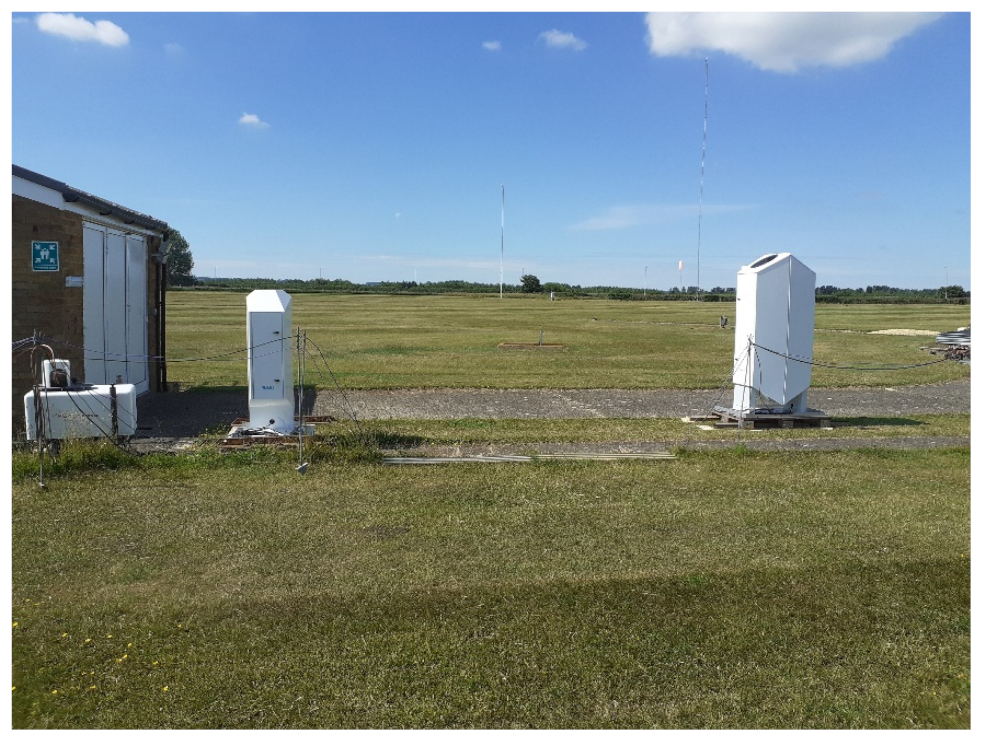
2.2. Campaign Setting

The BB-DIAL assessment period was from 15 June to 14 July 2020, during which time 93 Vaisala RS41 radiosondes were launched nearby (within 100 m). A quadcopter UAV developed by the Met Office team at Cardington performed 26 flights over 5 days from a location very close (within 100 m) to the BB-DIAL. This UAV was equipped with a capacitive device manufactured by IST (HYT 271 [23]) for humidity measurements; a thermistor from thermometrics (NTC Type FP07 [24]) for the temperature, the sensor was shielded to avoid solar contamination; and a Bosch Sensortec digital pressure sensor (BMP 280 [25]). Unfortunately, this UAV could only be operated up to a height of 500 m during the assessment period. Each flight (ascent and descent) was typically around 15 min duration, with the instruments reporting every 0.05 s. Most of the radiosonde launches were performed during the daytime at 9, 12 and 15 UTC (Figure 2), to follow the building up of the convective boundary layer, with only a small number at night and in dry conditions at launch. All the UAV flights were completed during the daytime (Figure 2), and in dry conditions. A Vaisala CT25K ceilometer for cloud-based recording was routinely operating at Cardington, as well as surface-based sensors recording a range of additional meteorological variables, including a laser rain rate recorder (installed on 6 July 2020), a tipping bucket rain gauge, visibility and radiation sensors.

Cardington is located in the countryside in Bedfordshire, with no remarkable orography at 29 m above mean sea level. The weather in Bedfordshire was typical of a summer period for that temperate region, slightly warmer than average in June and slightly wetter too; July experienced 19% more rainfall than average (see

Table 2. Climatology for Bedfordshire compiled by the “National Climatological Information Centre (NCIC) at the Met Office”, from the surface observation network.

Bedfordshire	Maximum Temperature		Minimum Temperature		Mean Temperature		Rainfall		Sunshine		Rain Days (>1 mm)
	°C	°C	°C	°C	°C	°C	mn	%	h	%	Days	Days
	Actual	1981–2010 Anomaly	Actual	1981–2010 Anomaly	Actual	1981–2010 Anomaly	Actual	1981–2010 Anomaly	Actual	1981–2010 Anomaly	Actual	1981–2010 Anomaly
20 June	21	1.3	10.6	0.9	15.7	1.1	55.5	107	201.7	109	10.5	1.4
20 July	21.7	−0.7	11.9	0	16.8	−0.3	59.7	119	177.8	89	9.9	1.4

).

3. Data Analysis

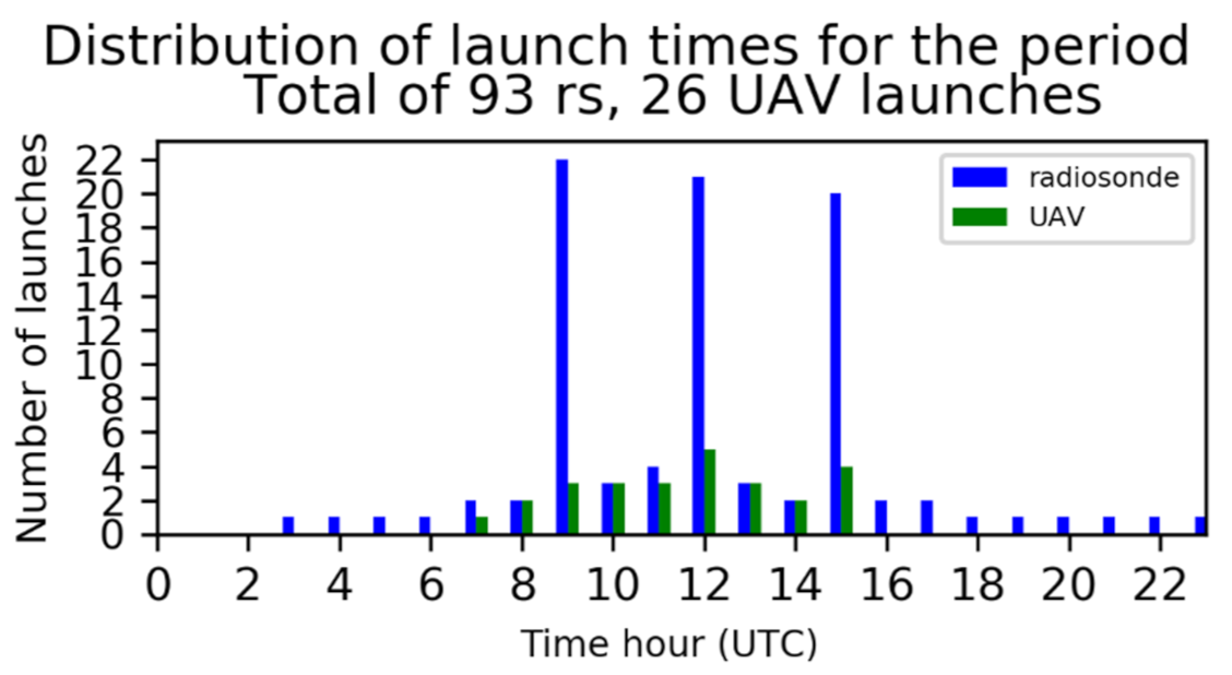
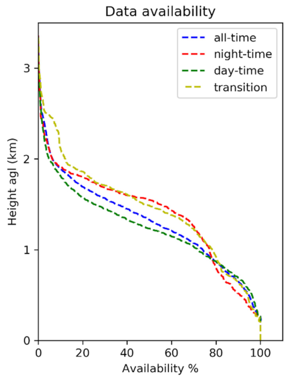
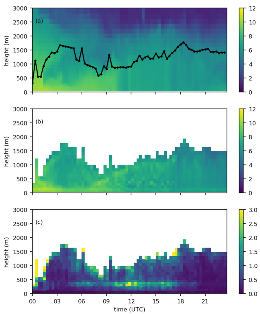
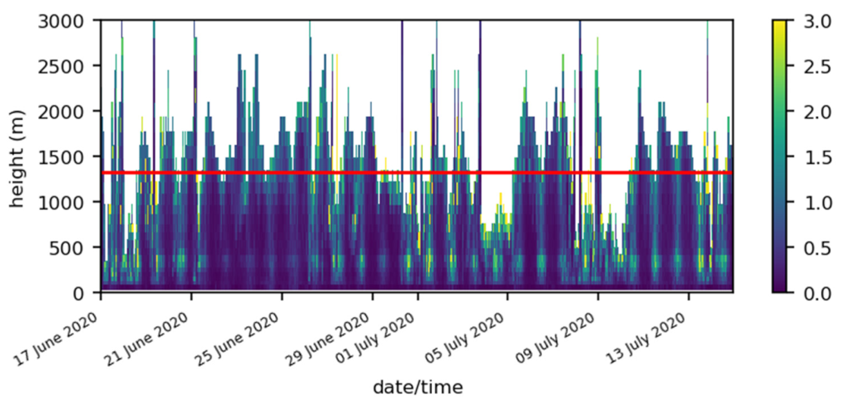
3.1. Data Availability

Figure 3 shows an example one hour time series of BB-DIAL mixing ratio and attenuated backscatter. In this example, the maximum range for the water vapour measurement is limited by the amount of aerosol. In the attenuated backscatter plot a sharp drop in aerosol can be seen at around 2 km and some cirrus clouds between 10 and 12 km. The BB-DIAL appears to be also a very powerful ceilometer

Figure 4 shows BB-DIAL data from an example dry day (29 June) and wet day (8 July). In general, the maximum height for the water vapour measurement is limited by thick cloud (see Figure 4a,e), with its impact on water vapour measurement height seen in Figure 4b,f). In clear sky, the maximum height for water vapour measurement varies between 1000 and 2000 m. For the wet day several episodes of rain occurred, with a laser rain recorder showing precipitation at ground level (Figure 4g). Comparison of Figure 4f with the timing of rain shown in Figure 4g shows that the instrument is able to measure in rain. For the event between 03:00 and 06:00 the laser cloud recorder shows a cloud base between 3000 m and 2500 m (Figure 4h), during which time there were BB-DIAL water vapour measurements up to that range. This is particularly interesting because a large variation in the water vapour mixing ratio with height is clearly captured (Figure 4f). This can be due to a change in temperature and air masses, but also due to non-adiabatic processes because of the rain.

During this experiment, data were missing for occasional short periods due to slow internet connection on the site. The data availability was computed using all data files which were not missing in the first gate. Figure 5 shows the maximum height considering all times of day, night-time only, daytime only and a transition period (defined as ±1 h around sunset and sunrise). Considering all times of day, data availability at 1000 m was 75%, falling to 35% at 1500 m. A 400 m increase in average data availability height was seen from day to night, with this increase occurring between 1000 m and 1800 m above the ground. For example, at 1500 m, availability at night was close to 55% but only 25% during the day-time. The overall average data availability height is 1300 m for the assessment period. These results are consistent with those published by Newsom et al. [16] and Mariani et al. [20].

3.2. Comparison of Water Vapour Mixing Ratio

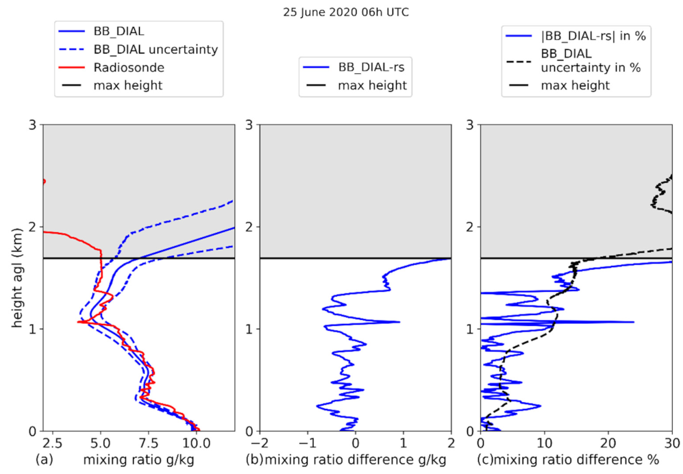
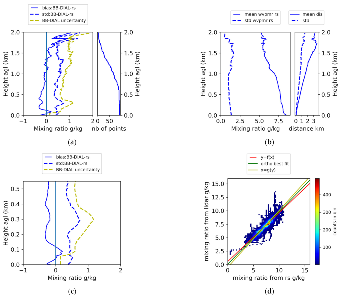
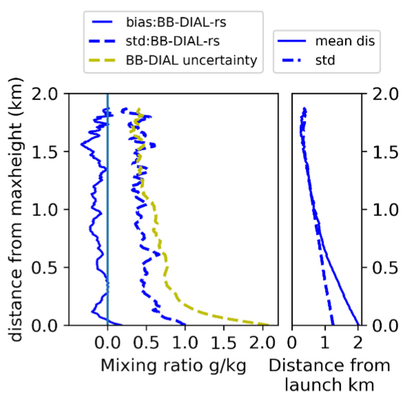
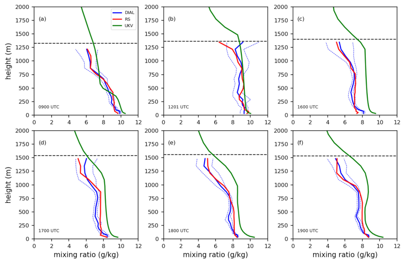
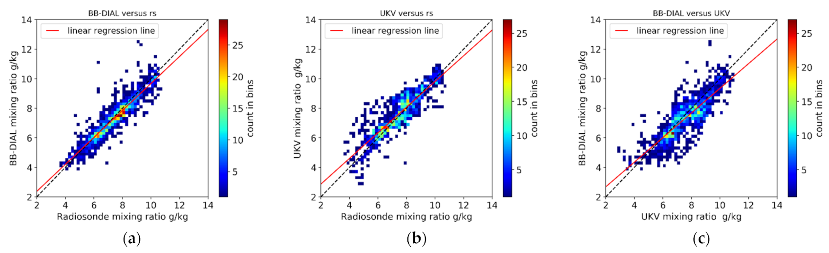
3.2.1. BB-DIAL versus Radiosonde

Radiosonde data with high vertical resolution (~5 m, 1 s data) have been used in this inter-comparison, with the values interpolated at the vertical reported BB-DIAL height (every 4.8 m). The Vaisala RS41 (successor of RS92) is classed as a high-quality radiosondes as defined by WMO [26]. While it remains challenging to get an absolute measurement of the humidity, the RS41 appears to perform slightly better than the RS92, with only a small dry bias of around 1% during daytime [27].

Figure 6 shows an example of the BB-DIAL mixing ratio, collocated in time (taking the middle of the 20-min time window) with a radiosonde ascent. The radiosondes were largely launched in the daytime, but with some ascents before sunrise and after sunset on a small number of days. The BB-DIAL reports data every 4.8 m, but as already mentioned in Section 2.1, the resolution increases from ~100 m at 50 m height up to ~500 m at ~3000 m. Therefore, the BB-DIAL profile is smoother than the radiosonde. It cannot represent the very sharp change at 1100 m above the ground, where the differences with the radiosonde measurements reach 24% (Figure 6c), or the step change at 1400 m and the small-scale variations between 400 m and 900 m. However, the BB-DIAL reproduces very well the broad characteristics of the radiosonde profile. The BB_DIAL captures well the decrease of the humidity between ~200 and 300 m but with a mismatch of 50 m in the height between the radiosonde and the BB_DIAL. The difference in this region reaches 10% around 260 m. Overall the difference between the radiosonde is in within a few % up to 1000 m. In the Figure 6 example, the BB-DIAL profile starts to diverge from the radiosonde measurement above 1400 m, with a general increase in the BB-DIAL uncertainty that reaches 18% at the maximum height (Figure 6c). The reported uncertainty is in good agreement with the measured difference from the radiosonde.

Over the whole assessment period, the bias between the BB-DIAL and the radiosonde remains small (Figure 7a). It is near 0 between 750 m and 1300 m, slightly negative below 750 m becoming quite variable below 500 m with two negative maxima of ~−0.32 g/kg at 200 m and 400 m. The bias becomes positive above 1700 m, but the significance of the result at this altitude is questionable as there were only 13 inter-comparisons with radiosondes at this height. The relatively strong variation of the bias in the first 100 m (from −0.27 to +0.20 g/kg) is mainly due to the BB-DIAL data in the lowest 50 m being the surface measurement (Figure 7c). Then just above 50 m, the bias becomes positive up to 100 m and then decreases and becomes negative with a maximum negative value at 200 m. The standard deviation remains small (less than 0.5 g/kg) except around 300 m, 1350 m and above 1800 m. At ~300 m, the standard deviation peak is 0.75 g/kg. Between 300 m and 400 m, which corresponds to the near and far field overlap region, the negative bias slightly increases with height.

Figure 7. Summaries of the comparison between BB-DIAL and the 93 radiosonde ascents for the entire evaluation period (15 June–16 July 2020): (a) bias (BB-DIAL-radiosonde), std deviation, BB-DIAL uncertainty variation with height and number of data points used; (b) climatology of the dataset: mean mixing ratio and standard deviation, (b) right: mean range from radiosonde launch point and standard deviation for the data used in the inter comparison; (c) zoomed on the lowest part of the radiosonde inter-comparison; (d) 2D histogram scatterplot BB-DIAL versus radiosonde, with corresponding statistics in

Table 3. Statistical results corresponding with the scatter plot in Figure 7d.

Number of Points	Correlation	Bias (BB-DIAL-Radiosonde)	RMS	Std Dev.
23071	0.93	0.10 g/kg	0.53 g/kg	0.52 g/kg

, (data every 4.8 m above 50 m have been used in 7 (d) and (Table 3).

Figure 7. Summaries of the comparison between BB-DIAL and the 93 radiosonde ascents for the entire evaluation period (15 June–16 July 2020): (a) bias (BB-DIAL-radiosonde), std deviation, BB-DIAL uncertainty variation with height and number of data points used; (b) climatology of the dataset: mean mixing ratio and standard deviation, (b) right: mean range from radiosonde launch point and standard deviation for the data used in the inter comparison; (c) zoomed on the lowest part of the radiosonde inter-comparison; (d) 2D histogram scatterplot BB-DIAL versus radiosonde, with corresponding statistics in Table 3, (data every 4.8 m above 50 m have been used in 7 (d) and (Table 3).

The BB-DIAL uncertainty, while larger than the standard deviation, follows the observed error very well. Compared to the climatology of humidity observed during the trial period, the error is well below the WMO OSCAR threshold of 10% and close to the breakthrough requirement of 5%. The overall bias is very small 0.1 g/kg, with a correlation of 0.93 with the radiosonde measurement. These results are in agreement with those published by Newsom et al. [16]: the correlation is slightly worse (0.93 vs. 0.97), but the standard deviation is lower (0.52 compared with 0.68). However, the data in the Oklahoma study spanned a larger range of humidity, with value up to 15 g/kg, so a larger standard deviation is expected.

For the overall bias which corresponds to only day time data (few radiosonde launches at night), there is a slight underestimation for the BB-DIAL mixing ratio compared to the radiosonde (−0.1 g/kg), whereas in the Oklahoma study [16] the bias was closer to zero (+0.2 g/kg). This result is encouraging as no radiosondes were used to calibrate the BB-DIAL prototype in this study, while in Newson et al. [16] the spectral width of the far field and near field used in the retrieval was adjusted to get the best fit with the radiosonde used also in the comparison, giving therefore a no biased solution. By using only data with the Vaisala BB-DIAL uncertainty lower than 1 g/kg, nearly all the outliers are removed, and the correlation increases to 0.95%. However, in doing so, the data availability is significantly reduced, with only 75% of the data remaining.

Because it was noticed that the discrepancy with the radiosonde increases towards the maximum height, the statistics have been recalculated versus the distance below maximum height. Figure 8 shows that the standard deviation increases to over 0.5 g/kg within 200 m below the maximum height. It also shows that the BB-DIAL uncertainty, while larger than the standard deviation, has a very similar profile shape. A possible mislocation in space between the radiosonde and the beam of the BB-DIAL might explain part of the increase in error. At the maximum height, the radiosonde is on average 2 km away from the BB-DIAL (Figure 8 right). On Figure 7a left, dash blue curve, there is no increase in the standard deviation above 1250 m when the radiosondes are, on average, more than 2 km away from the BB-DIAL (Figure 7b right, solid blue curve), so the effect of miss-location at the maximum height does not explain the increase in error. The increase in the offset in time only reaches 6 min at 2 km. This value remains negligible compared to the 20 min average of the BB-DIAL measurement. The BB-DIAL uncertainty follows the shape of the measured standard deviation and also increases when close to the maximum height. This confirms that there is a slight decrease in the BB-DIAL performance when close to the maximum height.

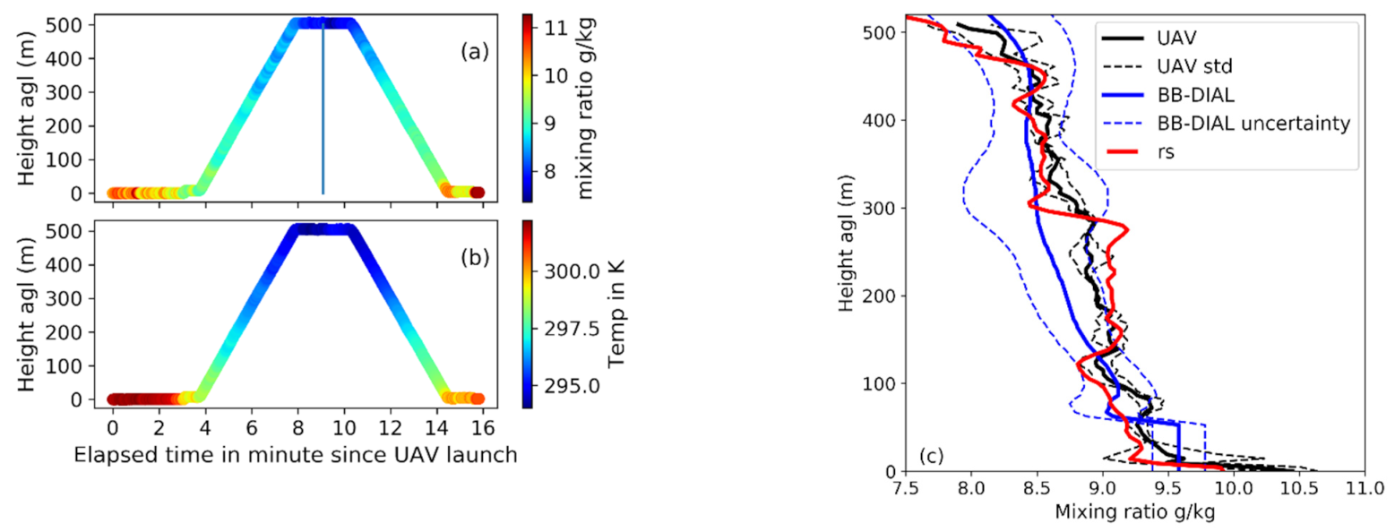
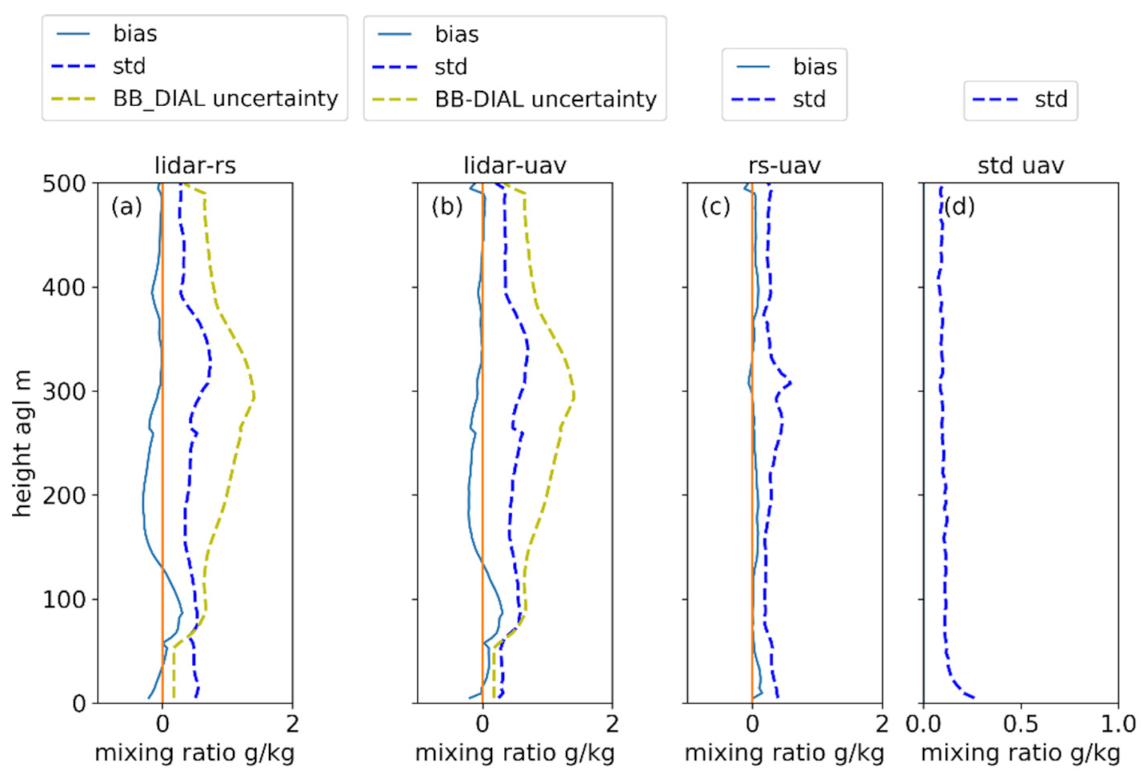
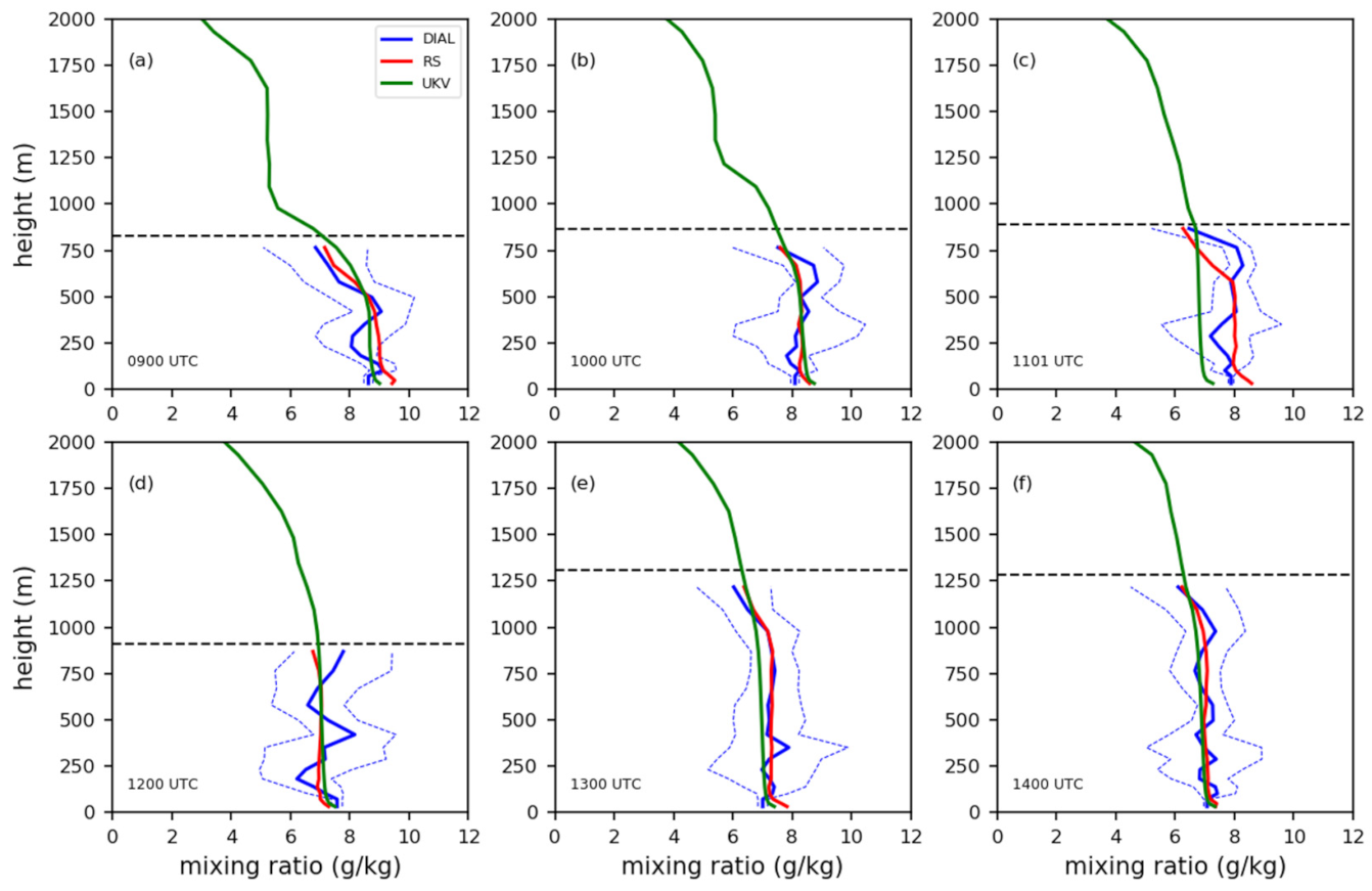
3.2.2. BB-DIAL versus UAV

The multicopter UAV completed 27 flights (ascent/descent) across 5 different days, with a radiosonde ascent coinciding with each UAV flight. The flights were completed at hourly intervals from 08 and 09 UTC to 15 UTC, from 07 to 12 UTC, and for 12 to 15 UTC, basically to capture the development of the convective boundary layer. Figure 9 shows an example of water vapour mixing ratio and temperature for a single UAV flight on 25 June at 09 UTC, along with the BB-DIAL and radiosonde measurements. In Figure 9c, the UAV mixing ratio data are averaged over 4.8 m, including ascent and descent data. This corresponds to around 100 measurements per 4.8 m bin. The time taken for the multicopter to span the 500 m is around 10 min. The solid black line is the average mixing ratio and the dashed black line the standard deviation for each 4.8 m sample. The agreement between the radiosonde, UAV and the BB-DIAL is generally good. The BB-DIAL profile is much smoother, with a tendency of slightly underestimating the water vapour mixing ratio in this particular case. There are small-scale differences between the UAV and the radiosonde, which could be genuine variability in the humidity or may be random noise in the UAV measurements. In addition, the sharp change in the water vapour mixing ratio reported by the radiosonde between 280 m and 300 m is not present in the UAV profile.

Figure 10 shows the inter-comparison of the three instruments for all the UAV flights completed. The bias of the BB-DIAL against the radiosondes and the UAV are very similar. There is an increase in the standard deviation of the UAV measurement in the first 20 m (Figure 10d), suggesting these measurements are slightly more variable than the rest of the profile, which shows a very small random noise. Above 50 m, the BB-DIAL bias shows the same oscillation mentioned in the comparisons with the radiosondes for the full data set. BB-DIAL data below ~50 m should not be considered because they are the surface measurement. None of the measurements are perfect, while very close, UAV and radiosondes data show some differences which can be due to sensor and representativeness errors and also time collocation (there can be up to 15 min difference between the radiosonde launch time and the mid-point of the UAV flight). While there is an increase in the standard deviation between UAV and radiosondes at 300 m (Figure 10c), this does not fully explain the increased variability seen at 340 m for the BB-DIAL between both UAV and the radiosonde.

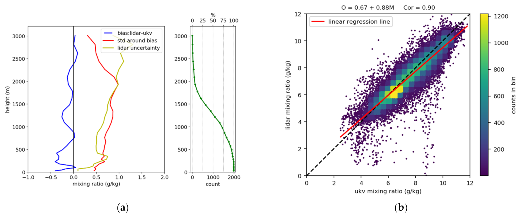
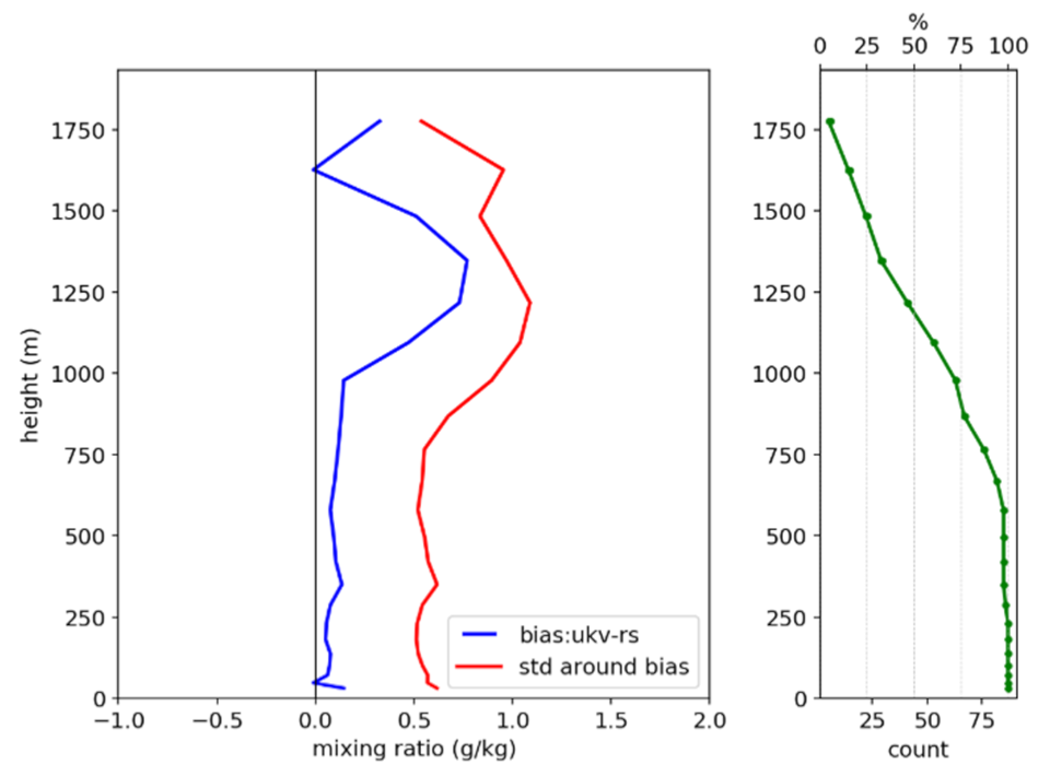
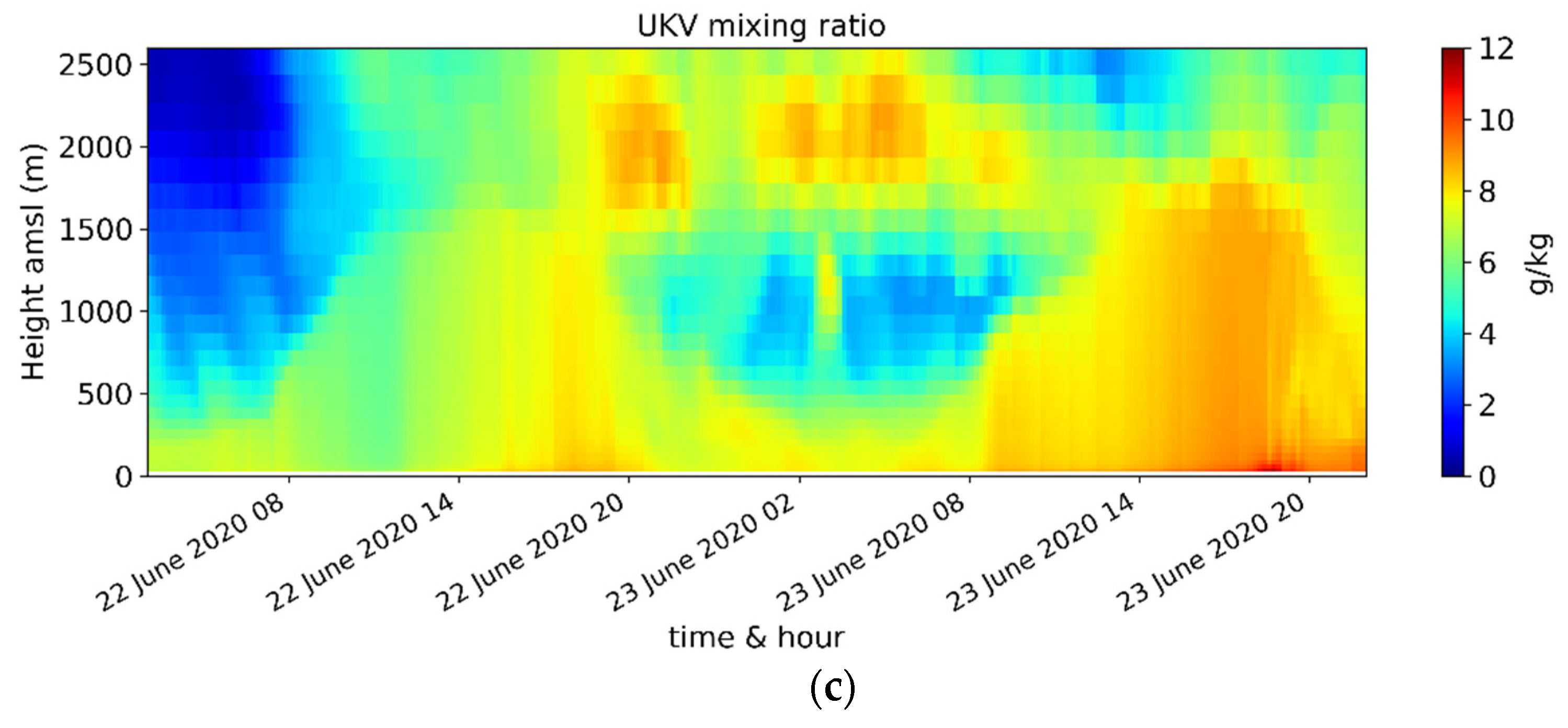
3.2.3. BB-DIAL versus UKV

The UKV is the Met Office’s high-resolution non-hydrostatic convection-resolving numerical weather predication (NWP) model [21]. It has a 1.5 km horizontal grid-spacing and 70 vertical levels, with a vertical resolution of 20 m close to the ground, increasing to 200 m at 3 km altitude. Operationally it is run at one-hour intervals. The UKV employs 4D-Var data assimilation [22] over a one-hour time window, with a 10 min time step within this time window. In the example shown in Figure 11 the UKV and BB-DIAL agree quite well, but with the UKV mixing ratio being slightly larger compared to the BB-DIAL. On the day illustrated (24 June 2020), several radiosondes were launched (Figure 12) which confirm that the UKV mixing ratio is an over estimation, particularly after 16:00. The BB-DIAL is in closer agreement with the radiosonde than with the UKV.

In the second example (14 July 2020) the BB-DIAL shows more structure in the lowest 500 m than the UKV, but the associated BB-DIAL uncertainty is also large (close to 3 g/kg) (Figure 13). As already mentioned, it is around 300 m that the standard deviation is largest when comparing with the radiosonde. There are visible oscillations in the BB-DIAL profile that are not present in the radiosonde (Figure 14). It is interesting to note that if the oscillations in the BB-DIAL profile are spurious, they are nevertheless well centred on the radiosonde profile, this is particularly true for the profiles at 12:00, 13:00 and 14:00 UTC.

In general, for the full 30-day period, the agreement with the UKV model is good, with a correlation of 0.90. While more negative than against the radiosonde, the bias compared with the UKV shows the same characteristics as against the radiosonde in the lowest 1000 m (Figure 15). As before, the lowest 50 m should not be considered, there is a sharp variation in the bias above 100 m similar to that seen in the radiosonde inter-comparisons. In the lowest 1000 m, the two local maxima (negative) in the bias are at around 240 m, and at 410 m. This is broadly similar to that observed in the radiosonde inter-comparison, taking into account that the comparison with the UKV is performed at 29 m above sea level. Another increase in the bias is seen at 1250 m. This increase is not present in the radiosonde inter-comparison where the bias is close to zero. The comparison between the UKV and radiosonde (Figure 16) shows a slight overestimation of the water vapour by the NWP model, with a larger bias around 1250 m, which also coincides with a larger standard deviation. This seems to indicate that part of this bias and some of the standard deviation is attributable to the UKV rather than the BB-DIAL. However, this result must be taken with caution because the radiosonde inter-comparison is just a sub-sample of the UKV model inter-comparison with relatively few data at this height.

With a correlation of 0.90, there is a good agreement between the BB-DIAL and UKV. However, some outliers do exist, and these have been found to be mainly data close to the maximum height.

3.2.4. Assessment of BB-DIAL and NWP Model versus Radiosondes

Using the BB-DIAL resolution mentioned in Newsom et al. [16], the radiosonde data have been averaged and then the value for the BB-DIAL and the radiosonde have been compared at each model level, values below 50 m have been excluded. The agreement between the radiosonde and the BB-DIAL is better than the UKV versus the radiosonde (Figure 17 and

Table 4. Statistical results corresponding with the scatter plots in Figure 17a,c.

No. of Points: 1454	BB-DIAL-Radiosonde	UKV-Radiosonde	BB-DIAL-UKV
Correlation	0.92	0.88	0.83
Bias	−0.099 g/kg	+0.149 g/kg	−0.248 g/kg
RMS	0.55 g/kg	0.69 g/kg	0.83 g/kg
Standard deviation	0.54 g/kg	0.67 g/kg	0.79 g/kg

). This is encouraging for the assimilation of the BB-DIAL. As already mentioned, (with some caution because of the small data sample at this height), the UKV bias observed around 1250 m could be reduced by the assimilation of BB-DIAL.

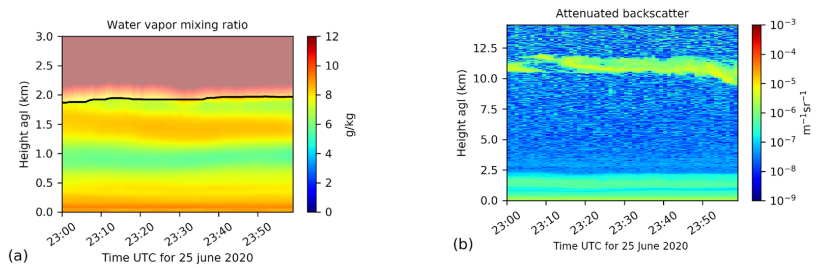
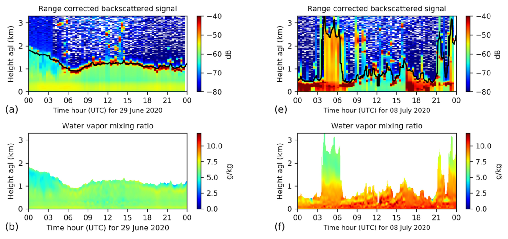
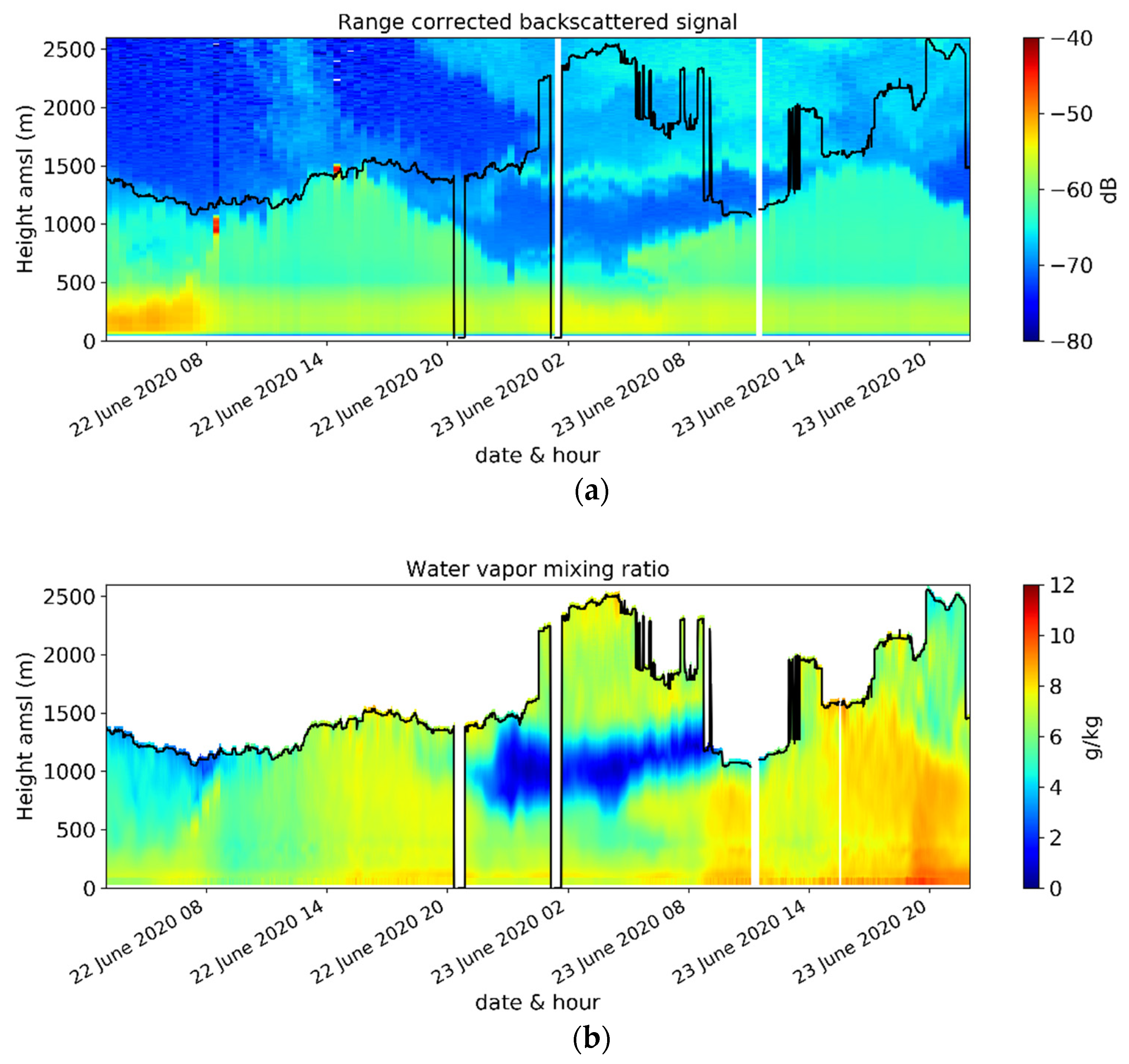
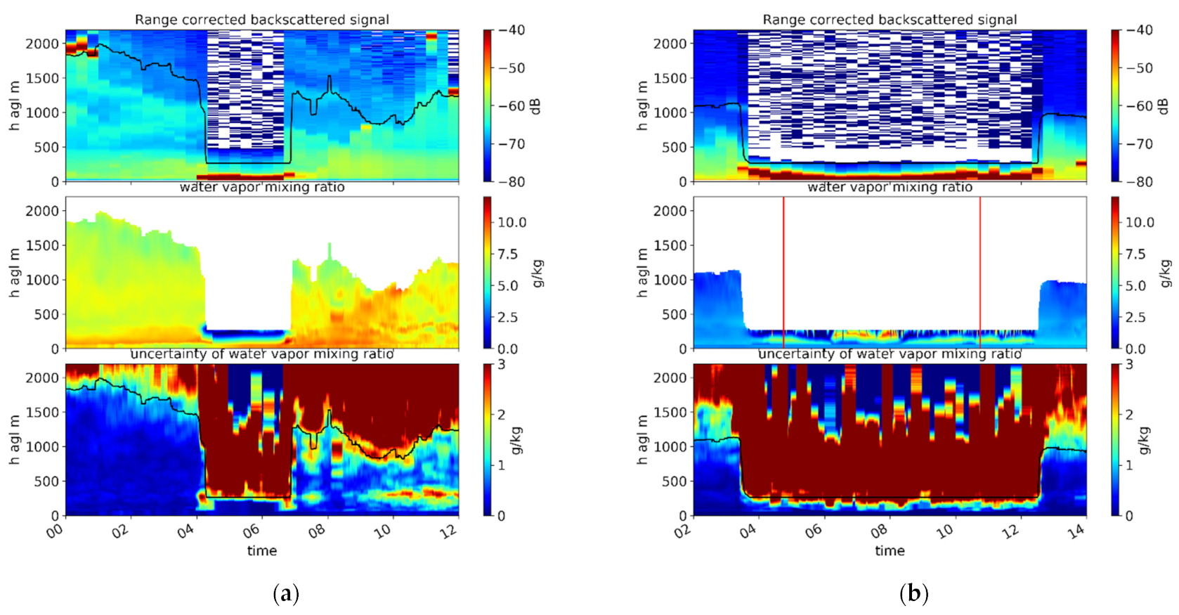
3.2.5. Capture of a Dry Layer in between Two More Moist Layers

Figure 18 show a very nice example overnight of a dry layer in between two more moist layers. Cardington was in a high-pressure system with a warm front further north. The UKV indicates a southerly flow in the lowest 500 m, then a westerly flow in the dry region and a south-westerly flow above. There is a temperature inversion at the bottom of the dry layer. While the general feature is captured by the UKV, sharpness and details are missing, and the UKV mixing ratio is still too high in the dry layer. Correct details of such features are important for the prediction of convective situations. In one of their examples, Browning et al. [28] indicate that a displacement of 150 m in the location of a lid is enough to initiate deep convection.

4. BB-DIAL Data Quality Issues Identified

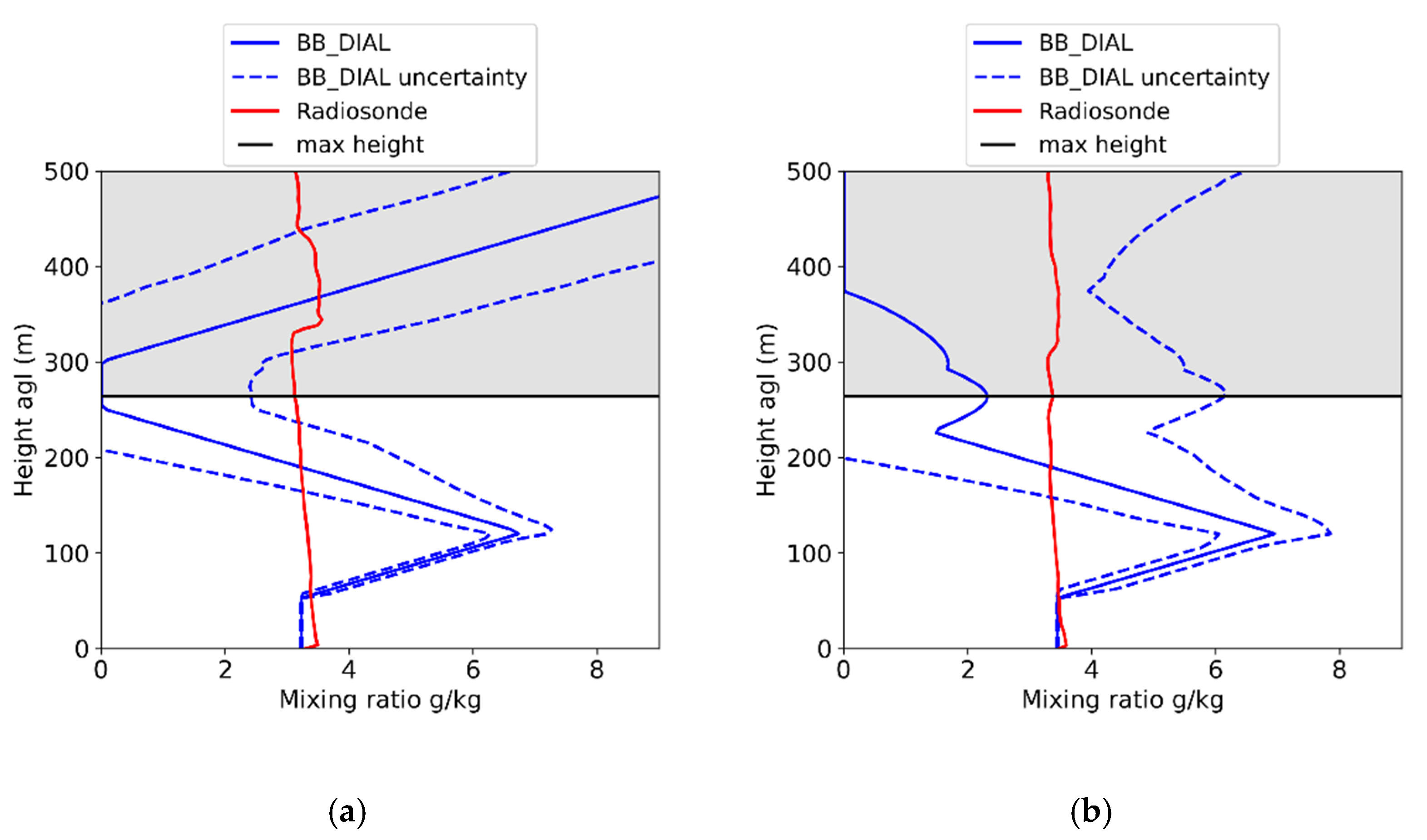
4.1. Lowest 500 m

As already mentioned, the lowest 50 m are not measured by the BB-DIAL but by the surface sensor. Vaisala proposes only giving the surface measurement and then the first BB-DIAL measurement at 50 m for the production model. Then just above, the bias is close to zero but increases quite sharply up to around 100 m and then decrease to become negative with a maximum at around 350 m, where both the bias and the standard deviation are maximum. Such features are seen in all the inter-comparisons (radiosonde, UKV and UAV) and was also seen by Mariani et al. [17], it corresponds to the region of overlap between the near range and far range telescope. This confirms the BB-DIAL origin. Such error is relatively well estimated by the error reported by the instrument. The height time cross section over the full period of the BB-DIAL uncertainty (Figure 19) shows an increase around midday. Solar contamination increases the noise. Vaisala is working on optimising the blending of the data from the near and far field.

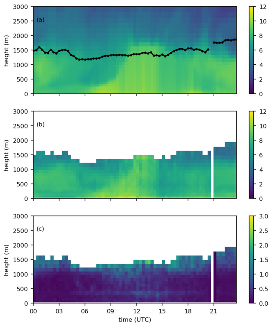
4.2. Spurious Oscillations

In situations when the mixing ratio does not change significantly in the vertical, the BB-DIAL profile often shows some pronounced oscillations, and the associated BB-DIAL uncertainty becomes larger. The oscillations appear to be random and centred on the true value (Figure 20) but are nevertheless spurious features. This could potentially result in the introduction of spurious features if the BB-DIAL data were assimilated. With a right error estimation, the assimilation scheme should filter such data, but it is not certain that the use of BB-DIAL uncertainty (which is large) in the assimilation process would reduce enough the weight of such spurious features. The fact that BB_DIAL uncertainty grows in such situation is useful. These oscillations are due to a reduced signal to noise ratio. It is possible that this issue can be partially resolved by modifying the sampling strategy, for example increasing the vertical resolution and/or increasing the time averaging.

There were a couple of fog situations during the assessment period: an example is shown in Figure 21. In this case, the BB-DIAL shows an extremely dry layer just above the fog (0.6 g/kg) which is most likely not a realistic feature. A similar feature was observed in a case from the BB-DIAL at Lindenberg (Figure 21b). In that event, collocated radiosondes verify that no such dry layer was found above the fog (Figure 22), the very humid layer at ~100 m above the ground is also in disagreement with the radiosonde measurement. For these cases, the maximum height should be specified significantly lower, at the cloud base, so for fog case at the surface. The feature is most likely due to signal saturation in the fog. Vaisala propose a solution by automatic gain control. As the signal is very stable the values were not rejected by the quality control, which is based on the variability of the signal inside the 20 min averaging window.

5. Discussion and Concluding Remarks

The BB-DIAL prototype was installed and configured by Met Office engineers at Cardington, following instructions provided by Vaisala, and ran without any required maintenance for a month. Although there were some short periods where data were missing due to local communications issues, the data were successfully archived for the entire period.

During the assessment period, the BB-DIAL was able to collect data in all weather situations, including in rain, when it was possible to have data up to the maximum reported height (3 km). The average BB-DIAL data availability height was 1300 m, with 76% of the data reaching 1000 m and 35% extending to 1500 m. The maximum height was significantly higher at night than during the daytime. The decrease of aerosol concentration and the reduction of signal to noise ratio with height limit the maximum range. Optically thick cloud also restrict the maximum range. In clear sky, the maximum range is between 1000 to 2500 m.

Compared with radiosonde humidity data, the bias is small and slightly negative. It has to be mentioned that the prototype BB-DIAL in this study does not use radiosonde calibration. The standard deviation is, on average, between 5% and 10%, which meets the WMO OSCAR threshold requirement for the accuracy and approaches the breakthrough requirement. The BB-DIAL uncertainty reported by the instrument is slightly higher than the standard deviation from the radiosonde comparison, but shows a similar trend with height. The error increases within 200 m of the maximum reported height, this is rather well captured by the reported uncertainty. For data assimilation an accurate observation error is essential [29], the fact that the trend against radiosonde is correct is very encouraging.

The comparison with the Met Office high resolution UKV is encouraging, with a correlation of 0.90. The error against the radiosonde is smaller than for the UKV against the radiosonde, so the BB-DIAL could potentially improve the model if assimilated. The UKV data show a rather large bias and large standard deviation against the radiosondes around 1250 m that could be reduced by the assimilation of the BB-DIAL data.

Despite the generally encouraging performance, a number of data quality issues were observed:

• The BB-DIAL data below 500 m show a variable bias with altitude and a large error against the radiosonde, the UKV and the UAV. The method of blending data from the near and far field overlap region could be explored as a means of mitigating this problem.
• The mixing ratio profiles frequently show oscillations, in particular when there is little change in the mixing ratio in the vertical. Such oscillations are relatively well captured by an increase of the reported BB-DIAL uncertainty but are nevertheless spurious features. Increasing the signal to noise ratio is something that could be explored in order to reduce this oscillation.
• The very dry layer reported above fog or thick cloud is not realistic. Utilising an automatic gain control is a possible solution to this issue.
• It should be clear that the lowest 50 m are surface instrument measurements, rather than based on information from the BB-DIAL. This is something that should be flagged in the data to ensure correct interpretation of the information.
• The instrument reports measurements every 4.8 m and every minute for smoother presentation but in practise, the resolution is much coarser, actually very close to the UKV model resolution for the vertical. It would be usefully to get the real vertical resolution at least in the form of metadata information.
• Data are averaged every 20 min. With a 10-min time step the UKV 4D-Var assimilation would probably benefit from a shorter averaging period. There is clearly a trade-off between accuracy and capturing variability in rapidly evolving situations.

Despite these issues, the overall results from this assessment are very promising. They suggest that this broadband BB-DIAL can generate vertical humidity profiles which can capture significant changes in humidity within the boundary layer. It is still premature to know if such measurements will add value to high resolution model, but the better agreement of BB-DIAL against the radiosonde, than UKV against radiosondes is encouraging. A longer period evaluation would be beneficial, possibly with BB-DIAL at more than one location, and including initial assimilation trials. The value of this data will increase if the data quality issues can be addressed or at least reduced to some extent.

References

1. Stone, E.K.; Pearce, G. A Network of Mode-S Receivers for Routine Acquisition of Aircraft-Derived Meteorological Data. J. Atmos. Ocean. Technol. 2016, 33, 757–768. [Google Scholar] [CrossRef]
2. De Haan, S. High-resolution wind and temperature observations from aircraft tracked by Mode-S air traffic control radar. J. Geophys. Res. Space Phys. 2011, 116, D10111. [Google Scholar] [CrossRef]
3. Wulfmeyer, V.; Hardesty, R.M.; Turner, D.; Behrendt, A.; Cadeddu, M.P.; Di Girolamo, P.; Schlüssel, P.; Van Baelen, J.; Zus, F. A review of the remote sensing of lower tropospheric thermodynamic profiles and its indispensable role for the understanding and the simulation of water and energy cycles. Rev. Geophys. 2015, 53, 819–895. [Google Scholar] [CrossRef]
4. Milan, M.; MacPherson, B.; Tubbs, R.; Dow, G.; Inverarity, G.; Mittermaier, M.; Halloran, G.; Kelly, G.; Li, D.; Maycock, A.; et al. Hourly 4D-Var in the Met Office UKV operational forecast model. Q. J. R. Meteorol. Soc. 2019, 146, 1281–1301. [Google Scholar] [CrossRef]
5. Hoover, B.T.; Santek, D.A.; Daloz, A.-S.; Zhong, Y.; Dworak, R.; Petersen, R.A.; Collard, A. Forecast Impact of Assimilating Aircraft WVSS-II Water Vapor Mixing Ratio Observations in the Global Data Assimilation System (GDAS); UW SSEC Publication 16.02.H1/Project Report; University of Wisconsin: Wisconsin, MW, USA, 2016; 38p, Available online: http://library.ssec.wisc.edu/research_Resources/publications/pdfs/SSECPUBS/SSEC_Publication_No_16_02_H1.pdf (accessed on 20 October 2021).
6. Petersen, R.A.; Cronce, L.; Mamrosh, R.; Baker, R.; Pauley, P. On the Impact and Future Benefits of AMDAR Observations in Operational Forecasting: Part II: Water Vapor Observations. Bull. Am. Meteorol. Soc. 2016, 97, 2117–2133. [Google Scholar] [CrossRef]
7. Reen, B.P.; Dumais, R.E. Assimilation of Aircraft Observations in High-Resolution Mesoscale Modeling. Adv. Meteorol. 2018, 2018, 1–16. [Google Scholar] [CrossRef] [Green Version]
8. Bianco, L.; Friedrich, K.; Wilczak, J.M.; Hazen, D.; Wolfe, D.; Delgado, R.; Oncley, S.P.; Lundquist, J.K. Assessing the accuracy of microwave radiometers and radio acoustic sounding systems for wind energy applications. Atmos. Meas. Tech. 2017, 10, 1707–1721. [Google Scholar] [CrossRef] [Green Version]
9. Leuenberger, D.; Haefele, A.; Omanovic, N.; Fengler, M.; Martucci, G.; Calpini, B.; Fuhrer, O.; Rossa, A. Improving High-Impact Numerical Weather Prediction with Lidar and Drone Observations. Bull. Am. Meteorol. Soc. 2020, 101, E1036–E1051. [Google Scholar] [CrossRef] [Green Version]
10. Aviation Technique for Tracking Humidity through Aircraft Signals Wins Top European Award. 2019. Available online: https://www.meteorologicaltechnologyinternational.com/news/aviation/technique-for-tracking-humidity-through-aircraft-signals-wins-top-european-award.html (accessed on 20 October 2021).
11. Brenot, H.; Rohm, W.; Kačmařík, M.; Möller, G.; Sá, A.; Tondaś, D.; Rapant, L.; Biondi, R.; Manning, T.; Champollion, C. Cross-Comparison and Methodological Improvement in GPS Tomography. Remote Sens. 2019, 12, 30. [Google Scholar] [CrossRef] [Green Version]
12. Whiteman, D.N.; Demoz, B.; Rush, K.; Schwemmer, G.; Gentry, B.; Di Girolamo, P.; Comer, J.; Veselovskii, I.; Evans, K.; Melfi, S.H.; et al. Raman Lidar Measurements during the International H2O Project. Part I: Instrumentation and Analysis Techniques. J. Atmos. Ocean. Technol. 2006, 23, 157–169. [Google Scholar] [CrossRef] [Green Version]
13. Chazette, P.; Marnas, F.; Totems, J. The mobile Water vapor Aerosol Raman LIdar and its implication in the framework of the HyMeX and ChArMEx programs: Application to a dust transport process. Atmos. Meas. Tech. 2014, 7, 1629–1647. [Google Scholar] [CrossRef] [Green Version]
14. Flamant, C.; Chazette, P.; Caumont, O.; Di Girolamo, P.; Behrendt, A.; Sicard, M.; Totems, J.; Lange, D.; Fourrié, N.; Brousseau, P.; et al. A network of water vapor Raman lidars for improving heavy precipitation forecasting in southern France: Introducing the WaLiNeAs initiative. Bull. Atmos. Sci. Technol. 2021, 2, 1–21. [Google Scholar] [CrossRef]
15. Spuler, S.M.; Hayman, M.; Stillwell, R.A.; Carnes, J.; Bernatsky, T.; Repasky, K.S. MicroPulse DIAL (MPD)–A diode-laser-based lidar architecture for quantitative atmospheric profiling. Atmos. Meas. Tech. 2021, 14, 4593–4616. [Google Scholar] [CrossRef]
16. Newsom, R.K.; Turner, D.; Lehtinen, R.; Münkel, C.; Kallio, J.; Roininen, R. Evaluation of a Compact Broadband Differential Absorption Lidar for Routine Water Vapor Profiling in the Atmospheric Boundary Layer. J. Atmos. Ocean. Technol. 2020, 37, 47–65. [Google Scholar] [CrossRef]
17. Mariani, Z.; Hicks-Jalali, S.; Strawbridge, K.; Gwozdecky, J.; Crawford, R.; Casati, B.; Lemay, F.; Lehtinen, R.; Tuominen, P. Evaluation of Arctic Water Vapor Profile Observations from a Differential Absorption Lidar. Remote Sens. 2021, 13, 551. [Google Scholar] [CrossRef]
18. Yeung, W.L.; Chan, P.W.; Lehtinen, R.; Roininen, R.; Münkel, C.; Chiu, Y.Y. Observations of subtropical weather by a prototype water vapour LiDAR at Hong Kong Observatory. Weather 2020, 75, 244–251. [Google Scholar] [CrossRef]
19. Roininen, R.; Münkel, C. Results from continuous atmospheric boundary layer humidity profiling with a compact BB-DIAL instrument. In Proceedings of the Eighth Symposium on Lidar Atmospheric Applications, Seattle, WA, USA, 26 January 2017; Available online: https://ams.confex.com/ams/97Annual/webprogram/Paper301717.html (accessed on 20 October 2021).
20. Mariani, Z.; Stanton, N.; Whiteway, J.; Lehtinen, R. Toronto Water Vapor Lidar Inter-Comparison Campaign. Remote Sens. 2020, 12, 3165. [Google Scholar] [CrossRef]
21. Rawlins, F.; Ballard, S.P.; Bovis, K.J.; Clayton, A.M.; Li, D.; Inverarity, G.W.; Lorenc, A.C.; Payne, T.J. The Met Office global four-dimensional variational data assimilation scheme. Q. J. R. Meteorol. Soc. 2007, 133, 347–362. [Google Scholar] [CrossRef]
22. Rothman, L.S.; Gordon, I.E.; Barbe, A.; Benner, D.C.; Bernath, P.E.; Birk, M.; Boudon, V.; Brown, L.R.; Campargue, A.; Champion, J.P.; et al. The HITRAN 2008 molecular spectroscopic database. J. Quant. Spectrosc. Radiat. Transf. 2009, 110, 533–572. [Google Scholar] [CrossRef] [Green Version]
23. HYT271 Sensor. Available online: https://www.ist-ag.com/sites/default/files/downloads/hyt271.pdf (accessed on 20 October 2021).
24. NTC Type FP0. Available online: https://www.mouser.co.uk/pdfDocs/AAS-920-267D-Thermometrics-NTC-TypeFP07-041216-web.pdf (accessed on 20 October 2021).
25. BMP 280. Available online: https://www.best-microcontroller-projects.com/support-files/bst-bmp280-ds001-18.pdf (accessed on 20 October 2021).
26. World Meteorological Organization (WMO); Oakley, T.; Vömel, H.; Wei, L. Proceedings of the WMO Intercomparison of High-Quality Radiosonde Systems, Yangjiang, China, 12 July–3 August 2010; WMO: Geneva, Switzerland, 2011; Available online: https://library.wmo.int/index.php?lvl=notice_display&id=15531#.YL90v0zTWF5 (accessed on 20 October 2021).
27. Sun, B.; Calbet, X.; Reale, A.; Schroeder, S.; Bali, M.; Smith, R.; Pettey, M. Accuracy of Vaisala RS41 and RS92 Upper Tropospheric Humidity Compared to Satellite Hyperspectral Infrared Measurements. Remote Sens. 2021, 13, 173. [Google Scholar] [CrossRef]
28. Browning, K.A.; Blyth, A.M.; Clark, P.; Corsmeier, U.; Morcrette, C.; Agnew, J.L.; Ballard, S.P.; Bamber, D.; Barthlott, C.; Bennett, L.; et al. The Convective Storm Initiation Project. Bull. Am. Meteorol. Soc. 2007, 88, 1939–1956. [Google Scholar] [CrossRef]
29. Desroziers, G.; Berre, L.; Chapnik, B.; Poli, P. Diagnosis of observation, background and analysis-error statistics in observation space. Q. J. R. Meteorol. Soc. 2005, 131, 3385–3396. [Google Scholar] [CrossRef]
Figure 1. Vaisala BB-DIAL (on the right) installed at Met Office, Cardington, Bedfordshire, UK (14 June–15 July 2020), with a CT25K ceilometer on the left.
Atmosphere 12 01521 g001
Figure 2. Distribution of radiosonde (blue) and UAV (green) launch times during the inter-comparison period.
Atmosphere 12 01521 g002
Figure 3. Example of one-hour time series of (a) water vapour mixing ratio (the black line indicates the maximum height for trusted water vapour measurement) and (b) attenuated backscatter. Note that BB-DIAL backscatter was not calibrated in this study, so the unit is arbitrary.
Atmosphere 12 01521 g003
Figure 4. Contrasting examples of BB-DIAL data: left-hand side dry day (29 June) and right-hand side wet day (8 July). (a,e) are the range corrected backscatter (data have been thinned in time and height for plotting), the black line is the maximum trusted height given by the Vaisala algorithm. (b,f) are the water vapour mixing ratio (in (g/kg)). (c) is the tipping bucket rain gauge showing no rain on the 29 June, (g) is the rain intensity at the surface measured by the laser rain recorder for 8 July. (d,h) show cloud base height from the Vaisala CT25K ceilometer near the BB-DIAL.
Atmosphere 12 01521 g004aAtmosphere 12 01521 g004b
Figure 5. Data availability computed for different time periods: all times, night-time only, day-time only, and transition periods (±1 h around sunset and sunrise).
Atmosphere 12 01521 g005
Figure 6. (a) Example of BB-DIAL (blue) and radiosonde mixing ratio for the 25 June 2020 at 06 UTC, (b) is the difference between the BB-DIAL mixing ratio and the radiosonde mixing ratio, (c) in blue is the absolute difference (%) against radiosonde measurement, black dash-line is the BB-DIAL uncertainty in % against the BB-DIAL measurement. The horizontal black line is the maximum height trusted value.
Atmosphere 12 01521 g006
Figure 8. BB-DIAL bias, standard deviation and reported uncertainty versus radiosonde as a function of distance below the maximum reported height. The mean distance from the radiosonde location point and standard deviation is shown on the right-hand panel.
Atmosphere 12 01521 g008
Figure 9. UAV, BB-DIAL and radiosonde inter-comparison, ~09:00, 25 June 2020. UAV flight time-height cross section for (a) mixing ratio and (b) temperature. The vertical blue line in (a) is the mid-point of the flight used for the time collocation with the BB-DIAL data. (c) Mixing ratio vertical profile for BB-DIAL (blue), BB-DIAL uncertainty (blue dash), radiosonde (red) and UAV (black). The UAV ascent and descent mixing ratio data are averaged over 4.8 m. The solid black line is the average mixing ratio and the dashed black line the standard deviation for this sample of typically around 100 values.
Atmosphere 12 01521 g009
Figure 10. Comparison (bias solid line, standard deviation and BB-DIAL uncertainty (dash line), (a) BB-DIAL-radiosonde, (b) BB-DIAL-UAV, (c) radiosonde-UAV. (d) is averaged standard deviation computed from each UAV sample (i.e., within a 4.8 m bins).
Atmosphere 12 01521 g010
Figure 11. Water vapour mixing ratio, 24 June 2020: (a) UKV model background; (b) BB-DIAL measurement thinned at UKV resolution (time and height); (c) BB-DIAL uncertainty, all values are g/kg.
Atmosphere 12 01521 g011
Figure 12. Water vapour mixing ratio profiles for different times on 24 June 2020: (a) 09:00 UTC, (b) 12:00 UTC, (c) 16:00 UTC, (d) 17:00 UTC, (e) 18:00 UTC, (f) 19:00 UTC. The horizontal dashed line represents the maximum height from the Vaisala algorithm.
Atmosphere 12 01521 g012
Figure 13. Example mixing ratio time-series for 14 July 2020: (a) UKV model background; (b) BB-DIAL estimation thinned at UKV temporal and vertical resolution; (c) BB-DIAL uncertainty, all values are g/kg.
Atmosphere 12 01521 g013
Figure 14. Water vapour mixing ratio profiles from BB-DIAL, radiosonde and UKV model background 09:00–14:00 UTC, 14 July 2020. The horizontal dashed line represents the maximum height from the Vaisala algorithm. (a) 09:00 UTC, (b) 10:00 UTC, (c)11:00 UTC, (d) 12:00 UTC, (e) 13:00 UTC, (f) 14:00 UTC.
Atmosphere 12 01521 g014
Figure 15. Comparison of BB-DIAL with the UKV model for the full assessment period. (a) Vertical profile of bias, standard deviation, BB-DIAL uncertainty and BB-DIAL data availability. (b) Scatterplot of BB-DIAL versus UKV, superimposed with a 2D histogram of the number of counts.
Atmosphere 12 01521 g015
Figure 16. Comparison of UKV with radiosonde (for comparison with Figure 15a) where BB-DIAL data are available.
Atmosphere 12 01521 g016
Figure 17. Scatter plots (in the form of 2D histograms). Note that the radiosonde data have been averaged at the BB-DIAL resolution (as provided by Newsom et al. 2020) at each model level and value below 50 m have been excluded. (a) BB-DIAL versus radiosonde. (b) UKV versus radiosonde. (c) BB-DIAL versus UKV.
Atmosphere 12 01521 g017
Figure 18. (a) range corrected backscatter, (b) BB-DIAL mixing ratio, (c) UKV mixing ratio.
Atmosphere 12 01521 g018aAtmosphere 12 01521 g018b
Figure 19. Time height cross section for the full period of the BB-DIAL estimated uncertainty. The horizontal red line is the average height.
Atmosphere 12 01521 g019
Figure 20. Examples of unrealistic oscillations in the BB-DIAL estimated mixing ratio profile with coinciding radiosonde measurements. The horizontal line indicates the BB-DIAL maximum height. (a) 14 July 2020 14:00 UTC, (b) 15 June 2020 12:00 UTC4.3. Dry Layer Above Fog.
Atmosphere 12 01521 g020
Figure 21. (a) BB-DIAL data for 16 June 2020. Top: range corrected backscatter (log scale). Middle: mixing ratio (g/kg). Bottom: reported BB-DIAL uncertainty (g/kg) for Cardington, (b) same as (a) but for the 4 February 2019 at Lindenberg from a similar BB-DIAL, the vertical red lines represent the radiosonde launch times, (Data provided by Dr Knist Christine DWD/Lindenberg).
Atmosphere 12 01521 g021
Figure 22. (a) radiosonde at 4:45 and BB_DIAL data for the fog case on 4 February 2019 at Lindenberg, (b) the same for 10:45 (Data provided by Dr Knist Christine DWD/Lindenberg).
Atmosphere 12 01521 g022