Article

Exploring the Change in PM2.5 and Ozone Concentrations Caused by Aerosol–Radiation Interactions and Aerosol–Cloud Interactions and the Relationship with Meteorological Factors

1
Flight Academy, Civil Aviation University of China, Tianjin 300300, China
2
College of Safety Science and Engineering, Civil Aviation University of China, Tianjin 300300, China
*
Author to whom correspondence should be addressed.
Submission received: 9 November 2021 / Accepted: 26 November 2021 / Published: 29 November 2021

Abstract

:
Aerosols can interact with other meteorological variables in the air via aerosol–radiation or aerosol–cloud interactions (ARIs/ACIs), thus affecting the concentrations of particle pollutants and ozone. The online-coupled model WRF-Chem was applied to simulate the changes in the PM2.5 (particulate matter less than 2.5 μm in aerodynamic diameter) and ozone concentrations that are caused by these mechanisms in China by conducting three parallel sensitivity tests. In each case, availabilities of aerosol–radiation interactions and aerosol–cloud interactions were set differently in order to distinguish each pathway. Partial correlation coefficients were also analyzed using statistical tools. As suggested by the results, the ARIs reduced ground air temperature, wind speed, and planetary boundary height while increasing relative humidity in most places. Consequently, the ozone concentration in the corresponding region declined by 4%, with a rise in the local annual mean PM2.5 concentration by approximately 12 μm/m3. The positive feedback of the PM2.5 concentration via ACIs was also found in some city clusters across China, despite the overall enhancement value via ACIs being merely around a quarter to half that via ARIs. The change in ozone concentration via ACIs exhibited different trends. The ozone concentration level increased via ACIs, which can be attributed to the drier air in the south and the diminished solar radiation that is received in central and northern China. The correlation coefficient suggests that the suppression in the planetary boundary layer is the most significant factor for the increase in PM2.5 followed by the rise in moisture required for hygroscopic growth. Ozone showed a significant correlation with NO2, while oxidation rates and radiation variance were also shown to be vitally important.

1. Introduction

Ozone–chemistry-related issues have now sparked a heated discussion among environmental scientists throughout the world [1,2,3,4]. As far as China is concerned, the fast-paced increase of ozone pollution in major cities across the country has become quite alarming, along with the issue of relatively high PM2.5 concentrations [5,6]. Therefore, the interplay between aerosols and gas pollutants is quite concerning, given the noteworthy presence of regional fine particles [7]. The point lies in reducing PM2.5 pollution while preventing ozone pollution from continuously increasing based on understanding how pollutants develop and build up with scientific evidence gathered from in situ measurements and numerical simulations. In the course of new developments in these directions, many articles have been published about how aerosol interacts with ozone pollution from a regional perspective.
In previous studies, an investigation was conducted into the correlation between particulate matter and ozone from different angles. A long-time measurement campaign was conducted in a northern city in China on a long-term basis. According to the results, the high level of PM2.5 in winter exerted an inhibitory effect on ozone, while meteorological variables such as temperature and humidity can cause the regional pollution of PM2.5 and ozone [8]. The findings made in this study also reveal the conversion rates of particles and their interactions with ozone. A comparison between different elements unravels the different mechanisms that are behind the absorption and distribution of the aerosols that are affecting the severity of ozone pollution. Additionally, other scholars have produced evidence for the different seasonal impacts of ozone pollution through aerosol loading [9,10,11]. Studies have also revealed [12,13] that HO2 radicals and other precursors are important in the atmosphere, and their uncertainties should be underlined in quantification and numerical simulations. Since NOx can serve as the precursor of ozone pollution and can play a significant role in the level of regional PM2.5 concentrations [14], the mechanism of the combined pollution on a local scale has triggered further discussions about local aerosol feedback along with a variety of other variables.
In fact, aerosols are significant to the change in atmospheric radiation budget and cloud nuclei to further adjust other atmosphere-related variables such as temperature, relative humidity (RH), the thermodynamics of the planetary boundary (PBL), and so on. As for the wet-scavenging process of aerosol, it is subjected to the influence of variation in the air. It has been demonstrated in prior studies that the aforementioned aerosol–radiation interactions (ARIs) and aerosol–cloud interactions (ACIs) could make a substantial difference to meteorology [15,16,17]. Therefore, this could lead to a noticeable enhancement of particle pollution mass concentration in the atmosphere through various mechanisms [18,19,20]. The notable positive feedback on the radiation budget in the air, PBL height [21], humidity [22], characteristics of cloud condensation nuclei, and cloud albedo is contributory to the regional concentration of particles [23]. Some of the studies focus on either a high-pollution episode in a typical region or an elucidation of a typical pathway for adjusting the particle mass concentration through meteorological feedback. However, it remains unclear how effective the relevant variables are in changing ozone due to the feedback. The relative contribution of these factors remains obscure. Consequently, it is necessary to quantify the association of PM2.5 and ozone with ARIs and ACIs using appropriate numerical models. Since the physics and chemistry parts mutually interact through coding, a state-of-the-art on-line coupled chemistry transport model is considered as an ideal solution for quantifying the impacts of ARIs and ACIs on PM2.5 and ozone concentrations [24,25,26]. Moreover, model outputs can isolate the impact of different types of feedback from one another when sensitivity tests are conducted under the proper settings. The results that are obtained here may emphasize the significance of joint emission control in critical elements and the optimization of relevant policies.
The rest of the paper is structured as follows: The configuration and evaluation of the numerical model applied in the study are introduced in chapter two. Then, the evaluation of both the meteorological and chemical performance is conducted by comparing simulated and observed datasets. Chapter three illustrates the spatial distribution of changes in PM2.5 and ozone concentrations and elaborates upon the variables that are relevant to weather and atmospheric chemistry. This chapter also conducts a partial correlation analysis to assess the statistical relationship between different variables and quantified relationships. Due to the limitation on the scope of the paper and the cost of computing resources, there are some potential drawbacks to the study, which will be explored in the Discussion part of the paper along with some possible directions for further study.

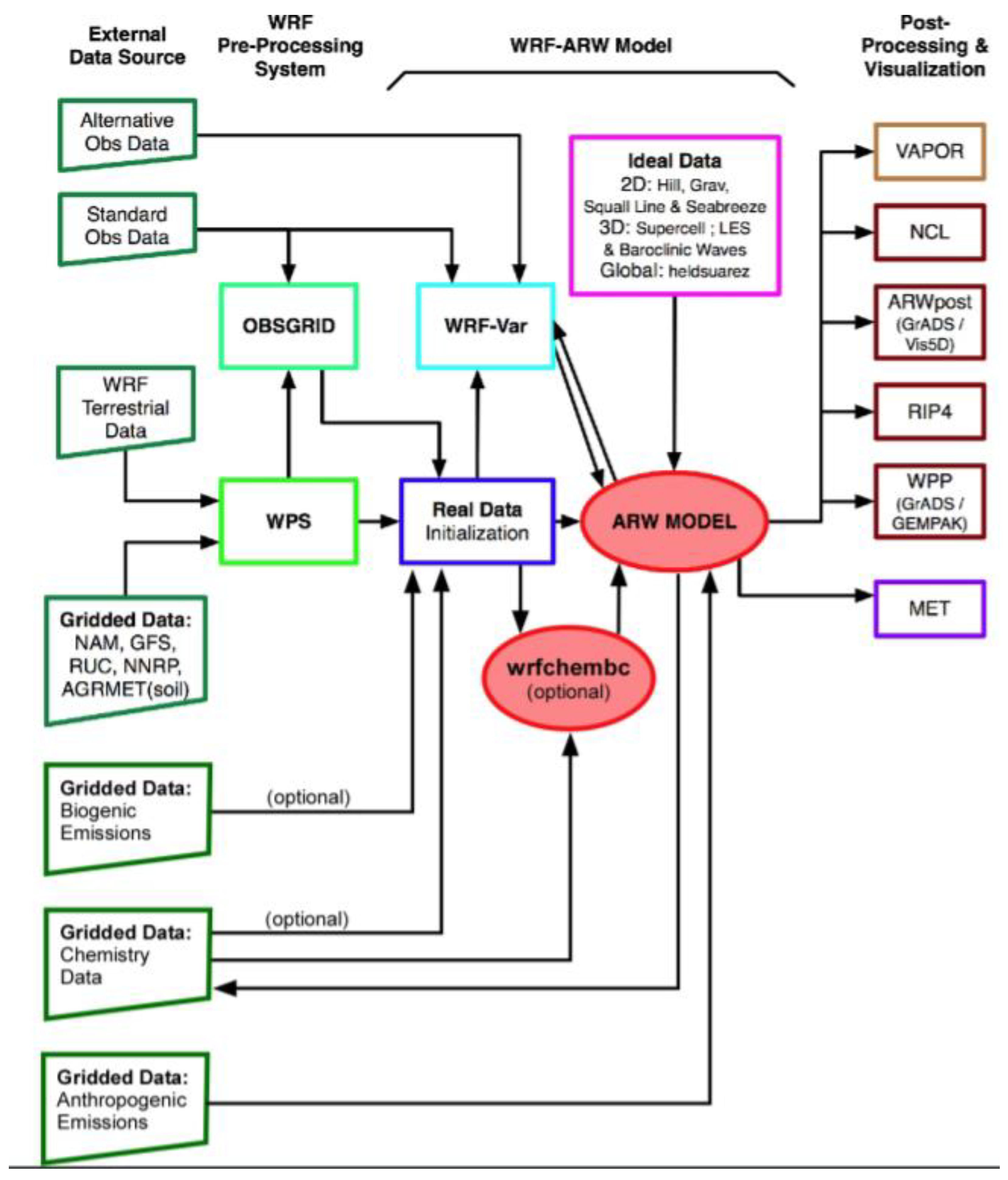
2. Model Configuration and Evaluation

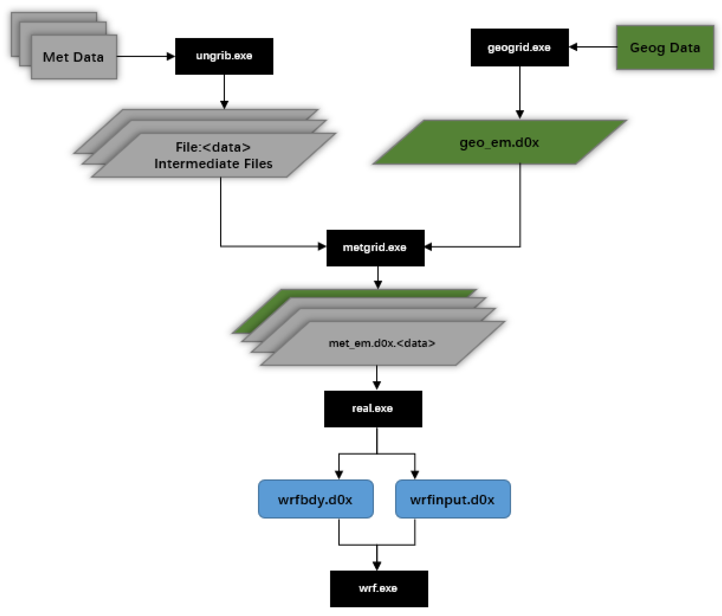
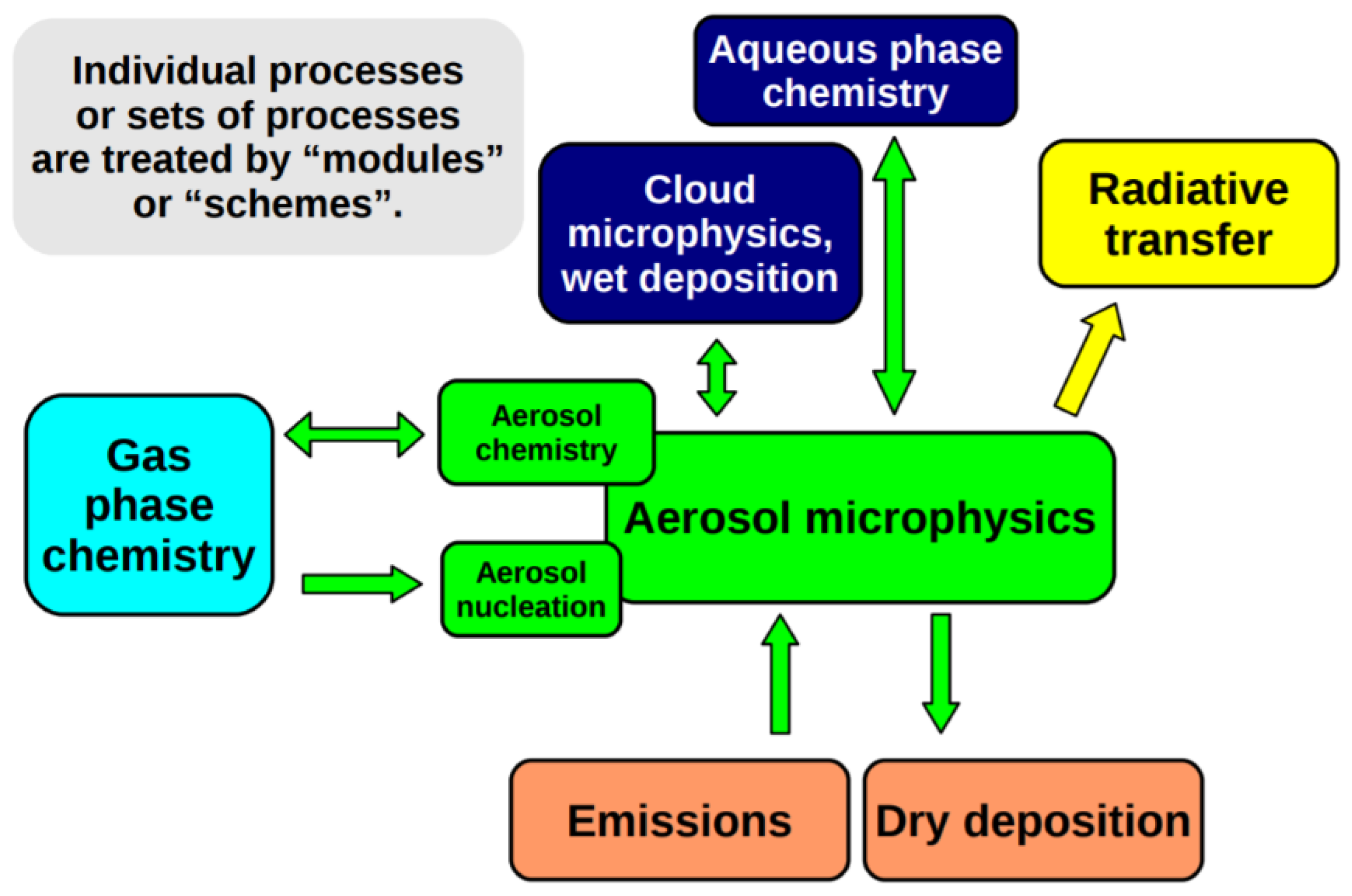
2.1. Model Setting and Design of Sensitivity Tests

The model WRF-Chem model was applied in the present study. It is an advanced atmospheric chemistry transport model that includes full aerosol feedback. It offers plenty of choices in terms of atmospheric physics and chemistry, with different parameterization schemes being available. The modules are set in the physics and chemistry packages of the model, where the codes are interconnected. In this way, physical factors such as temperature, air humidity, kinetic energy, and radiation that are present in different layers can interact with the chosen chemistry schemes, thus offering comprehensive feedback loops in both aerosol–radiation interaction and aerosol–cloud interaction. Therefore, it is an ideal solution for the feedback simulation [27].
To focus on the region of China, the simulation area is designed to cover the whole territory of mainland China and the vicinity of the Pacific Ocean, similar to our previous study [28]. The horizontal resolution of the study area is 36 km for each grid. Since the atmospheric processes are highly complex within the planetary boundary layer (PBL), lower air has more vertical layers than upper air, with the total number of vertical layers exceeding 40. January, April, July, and October are the four months that were deliberately chosen to represent the four seasons. In each simulation, a one-week spin-up was carried out one month before the study to ensure that the study was able to obtain proper results. The initial and boundary conditions for the simulation were derived from NCEP FNL (final analysis) data, which can be freely downloaded from a link on the official site of the WRF. Additionally, the sea surface temperature (SST) data were updated on a daily basis as a lower boundary in order to provide inputs so that the model could conduct correct calculations. The chemical boundary condition was determined by MOZART, as recommended by the WRF-Chem group; this method has been commonly accepted as a suitable solution for the organization of the proper data for chemical simulation. In this study, the anthropogenic emissions from the MEIC emission inventory [29] and the natural emissions from the MEGAN inventory created by Guenther [30] are treated as the emission inputs.
The following chemistry and physics modules were used in the WRF-Chem model in this study: The Rapid Radiative Transfer Model for GCMs (RRTMG) [31] was chosen for simulating both long-wave and short-wave radiation. The Morrison two-moment scheme was used for cloud microphysics [32], and the Kain–Fritsch scheme was used for cumulus convective parameterization [33]. The Noah land–surface scheme [34], the Monin–Obukhov surface scheme [35], and the Yonsei University planetary boundary layer (PBL) scheme [36] were used for the lower boundary conditions in the study. The chemical mechanism that was used was the Carbon-Bond Mechanism version Z mechanism in the Model for Simulating Aerosol Interactions and Chemistry (CBMZ/MOSAIC) using four sectional aerosol bins, including some aqueous reactions. To represent photochemistry, the Fast-J photolysis scheme was used [37]. The options above are able to represent feedback [38,39,40,41] and are adequate for the present study.
As mentioned above, the city clusters in China are crucial for exploring complex PM2.5 and ozone pollution. To collect the specific data required for further calculations, five typical regions distributed across China were selected to represent different parts of China. The locations of the North China Plain (NCP), Sichuan Basin (SCB), Lianghu Plain (LHP), Yangtze River Delta (YRD), and Pearl River Delta (PRD) are marked in boxes, as shown in Figure 1. From the north to the south, they cover different weather characteristics, and the numbers of ground-based meteorological sites as well as the national environmental observation sites in China are adequate for further statistical evaluation, as listed in Table 1.
A detailed model configuration and an explanation of the calculation process inside of the model can be found in the Appendix A.
Three parallel sensitivity tests were performed in the study to quantify the difference in the ARIs and ACIs in the atmosphere, as shown in Table 2. Because it consists of full feedback, the first test means that ARIs and ACIs are both considered in the simulation. It is therefore called BASE. As for the second test, it excludes the ACIs by setting the cloud droplet number to a constant number in the code of the corresponding cloud microphysics scheme. With only radiation feedback open, this test is called RAD test. In the third test, both the ARIs and ACIs are excluded by fixing the cloud droplet number and by turning off ARIs in the namelist at the same time, thus it is called NON. In this way, the differences between the first and the second tests can be solely attributed to ACIs, while the differences between the third and the second tests only result from ARIs. This method has been widely applied in prior studies exploring the effects of ACIs and ARIs [16,17,18,19,20,21,23,24,25,26,27].

2.2. Model Evaluation

Before any further analysis of the model output, it is necessary to thoroughly assess model performance in the first place. In general, the evaluation results that are shown for the study are classified into two categories: meteorological evaluation and chemistry evaluation. In each category, relevant factors are compared against observational datasets to present the statistical results.

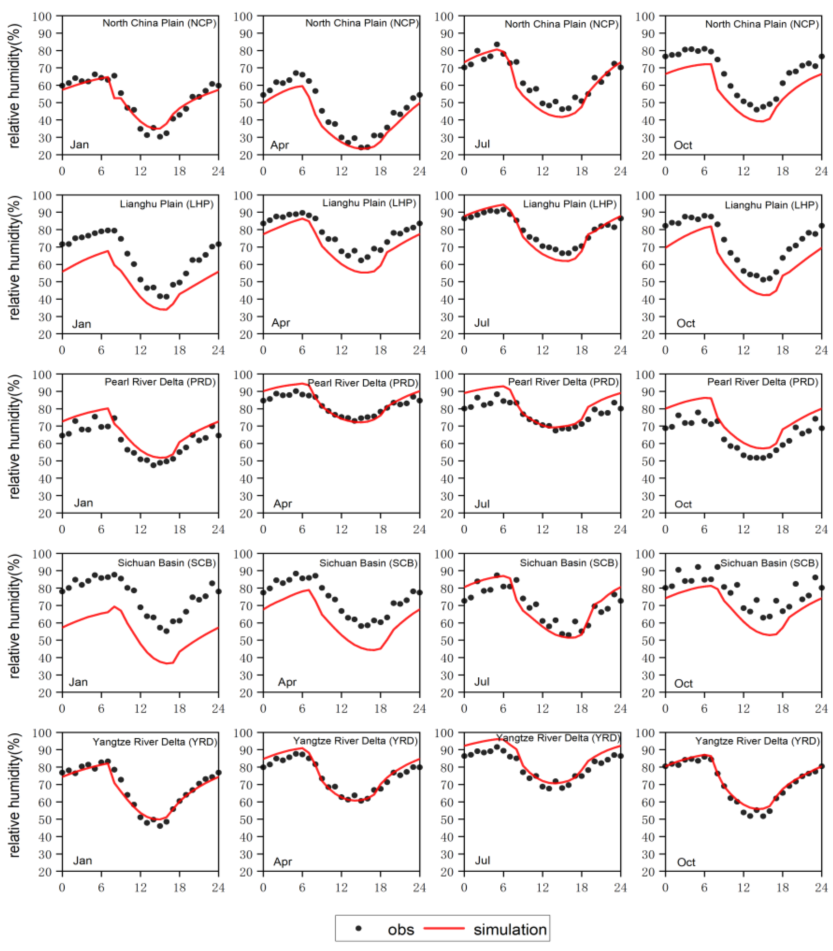
2.2.1. Evaluation of Meteorology

As for meteorological evaluation, there are several main parameters that should be calculated in the atmosphere compared to ground measurements. The statistical assessment involves as many as thousands of meteorological sites within the whole domain. The data retrieved from the ground measurements are sourced from the National Climate Data Center (NCDC) and are available to download via the link provided by the authority based in the U.S. (https://www.ncei.noaa.gov/, accessed on 30 June 2021).
In Table 3, the mean observation values, mean simulation values, correlation coefficients, and other statistical results, including mean bias, normalized mean bias, root mean square error, and normalized mean error are presented. As for the correlation coefficients of temperature and relative humidity (RH), they were determined to be 0.94 and 0.70 at air that is two meters about the ground, respectively. The normalized mean biases are −5.04% and 2.71%, respectively. The results are comparable or higher than the levels obtained for previous studies, indicating the model’s excellent performance in simulating the variables. The correlation coefficient of the simulated and observed wind speed and precipitation was 0.54 and 0.73, respectively, with wind speed being over estimated and the precipitation being underestimated.
To further identify the temporal distribution of the model performance, additional information is provided in Figures S1–S3 in the Supplementary Materials. The temporal trends of the simulated temperature, relative humidity, and wind speed show good agreement with the observations in the corresponding regions. Relatively larger relative humidity biases can be found in the Sichuan Basin and Lianghu Plain regions in the winter. Wind speed had a tendency to be underestimated in the south during summertime. One can refer to the diurnal characteristics of the variables in Figure 2 and Figure 3. The diurnal characteristics were calculated based on different regions in different seasons. The simulated results from the model output are shown, and the results are shown to have captured the diurnal trends of the variables well. However, biases can be found in the Sichuan Basin and North China Plain. The spatial distribution of the mean bias for precipitation in each month is illustrated in Figure S4. Most of the underestimated precipitation sites are concentrated in central and north China, while overestimates occur in the south and southwest of China during spring, summer, and autumn. In general, the model captures the features of the meteorological variables present in the simulation domain well, with the exception of some relatively larger biases in certain regions.

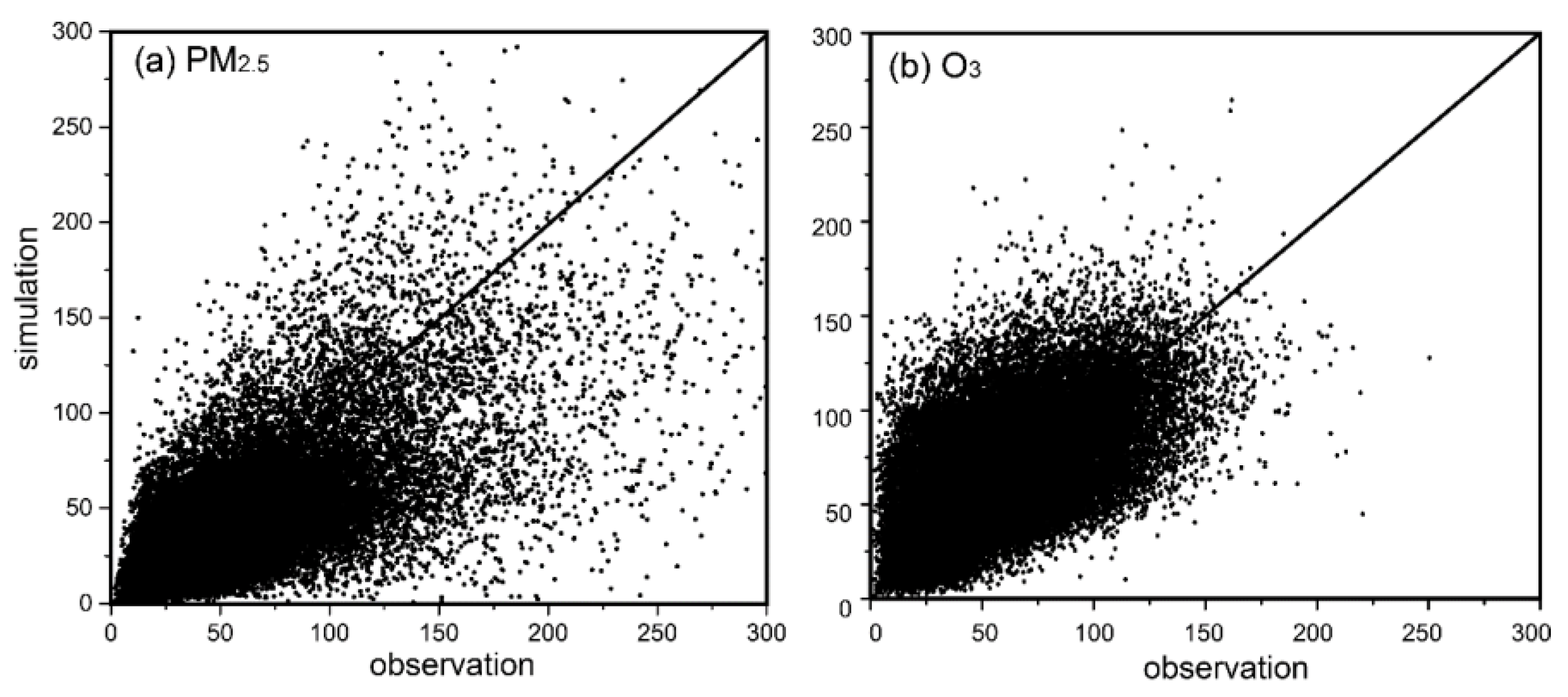
2.2.2. Evaluation of Chemistry

In addition to meteorological factors, the outputs of the chemical elements from the WRF-Chem model were compared as well. The observation dataset was from the China National Environmental Monitoring Center (CNEMC). The hourly observational air pollution mass concentration values in μg/m3 are compared with the outputs derived from the WRF-Chem model in Figure 4.
Figure 4 shows the simulated concentrations of PM2.5 and ozone compared to the observations. As suggested by the scatter plot, the level of model performance is satisfactory, with the correlations and biases being detailed in the Table. The PM2.5 concentrations are slightly underestimated, while ozone is slightly overestimated by the WRF-Chem model as a whole. Notably, every single dot in the scatter plot represents an hourly observational result with a corresponding simulation result in the grid within the domain. For clarification, grids are chosen from within five typical regions across mainland China, where the observational sites of CNEMC are available and are calibrated with quality control. In general, the scatter plot suggests an underestimated concentration of PM2.5 in panel (a) and an overestimated ozone concentration in panel (b). The Pearson correlation coefficients of PM2.5 and ozone are 0.689 and 0.575, both of which are above the 0.01 significance level. The figure indicates the good performance of the WRF-Chem model in simulating these two chemical variables.
Given the transportation of chemical elements between different regions, all of the sites located in mainland China that were available from CNEMC were compared against the corresponding simulation outputs that were derived from the WRF-Chem model. The statistical results of CO, NO2, SO2, PM10, PM2.5, and O3 are all listed in Table 4 and are separated by month. Briefly, the biases of the particulate matters and CO are negative, while the other variables are positive. There are relatively large biases found in January, a month when the majority of east China experienced severe pollution. In other months, the biases are less significant.
To summarize, the model can reproduce the meteorology and chemistry in the domain well even though some biases are present for certain elements during certain periods.

3. Results

In the previous chapter, the performance of the WRF-Chem model was discussed in detail. The results are consistent with the conclusion that it performs well in capturing the meteorological and chemical characteristics. After a series of post-processing coding, the output files of the WRF-Chem model were examined to explore the reason for changes in multiple variables on the ground level.

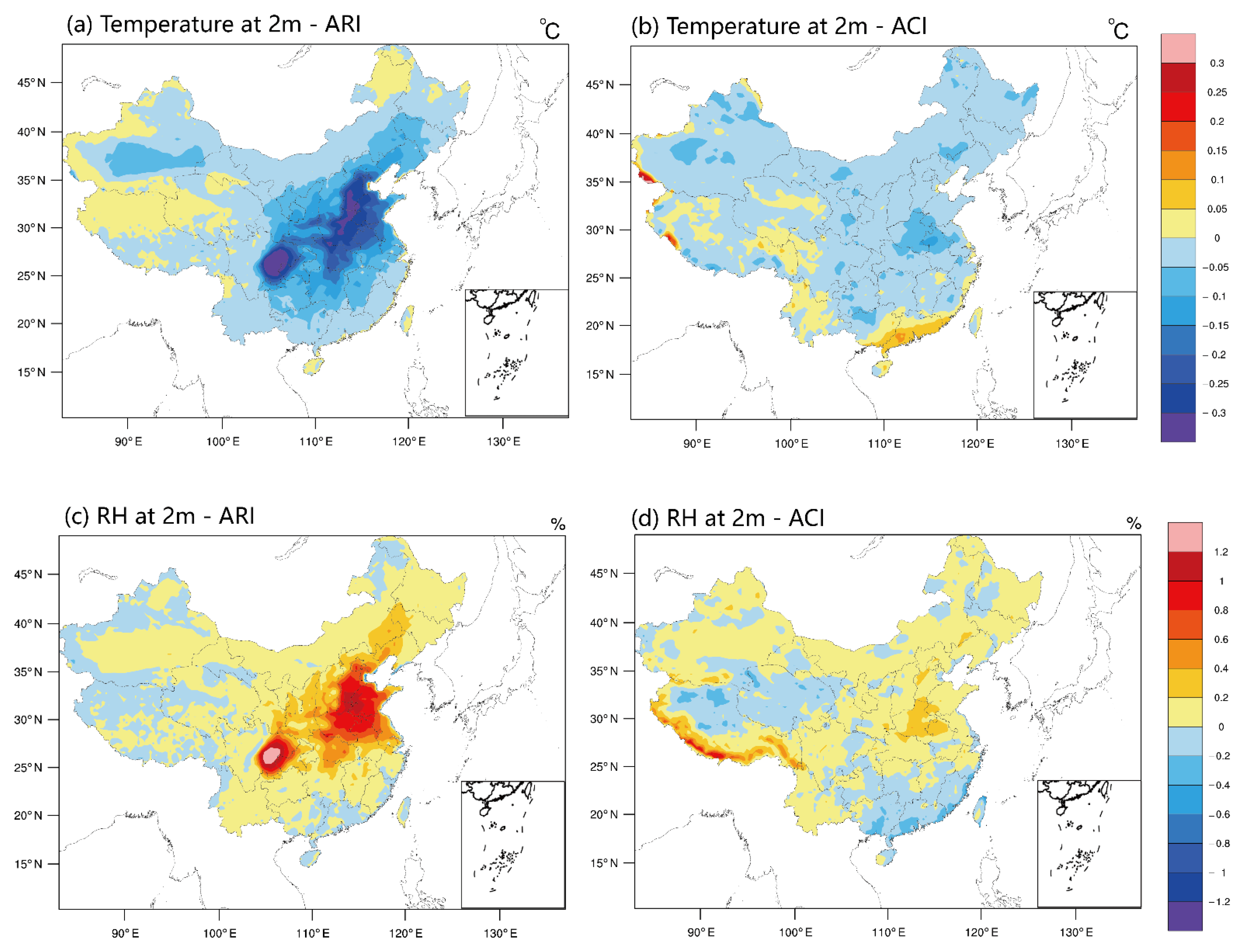
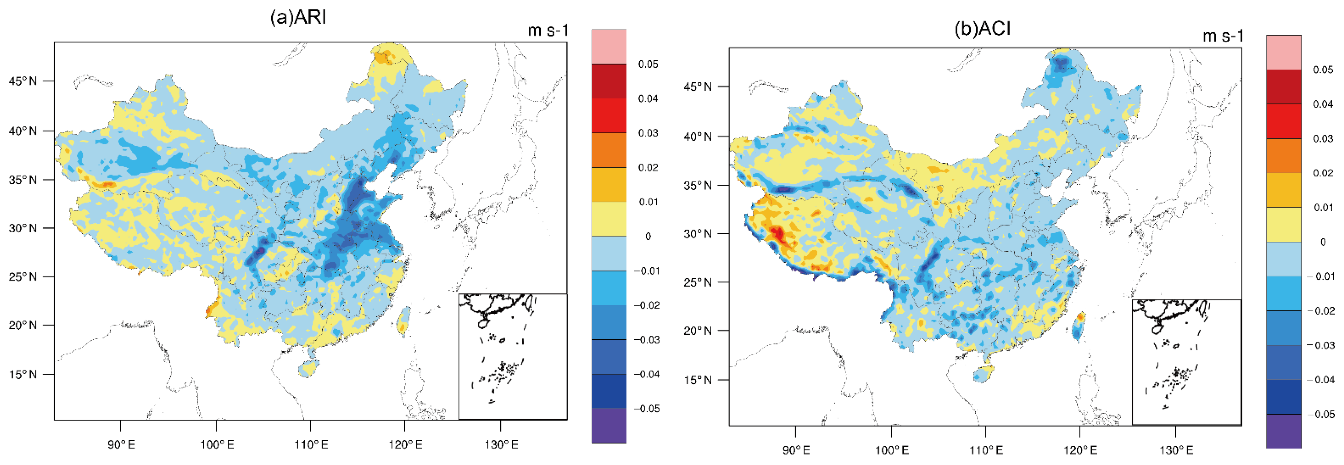
3.1. Changes of Meteorological Variables and Precursors

Because aerosols demonstrate absorbing and scattering characteristics in the air, heavy aerosol loading has been deemed contributory to reducing the solar radiation that is received on the surface of the planet. If aerosols are involved in the cloud formation mechanism as nuclei, then radiation variance also exists. Therefore, a comparison of the net solar radiation on the surface layer caused by ARIs and ACIs is shown in Figure 5. It is easy to identify the fundamental differences in the spatial distribution of changes in the intensity of shortwave radiation due to ARIs or ACIs. If aerosols are irrelevant to cloud microphysics, then the cloud droplet number across the domain is constant, so changes in the surface radiation can only result from ARIs, as shown in panel A. The sharp decline in the annual mean of the solar radiation received on the ground is concentrated in those densely-populated city clusters across China, within northern and central China in particular, where a maximum of over 22 W/m2 reductions can be observed within one year. However, the change caused by ACIs is a separate issue. In central and northern China, the feedback via ACIs contributes to increasing the shortwave radiation received on the surface by 0.8–1.6 W/m2. Meanwhile, the reduction of the radiation can be observed in some parts of the Sichuan Basin and in southern China by up to −1.8 W/m2. The spatial distribution of changes in radiation due to ACIs shows a clear divide along the south bank of the Yangtze River, where the north is positive, and the south is negative. It is worth noting that the extent of changes in radiation that are caused by ACIs is far less significant than the changes that are caused by ARIs, with a gap that is approximately 10 times larger.
The alternation of the radiation received at the surface layer via ARIs and ACIs can make a difference to both ground air temperature and relative humidity. As shown in Figure 6, the majority of China experienced lower temperatures when ARI or ACI feedback was considered. However, the extent of temperature change at an annual mean level can vary due to the different pathways of interaction. The temperature changes can reach up to −0.3 ℃ due to ARIs in the Sichuan Basin, but only a maximum reduction of −0.1 ℃ can be found in panel B due to ACIs. Panels C and D illustrate the changes in RH that are caused by ARIs and ACIs, respectively. Moreover, there is an evident rise in RH in most parts of central and eastern China, with the most significant increase being found in SCB. Relative humidity is calculated by the water vapor pressure divided by the saturation vapor pressure. In fact, saturation vapor pressure is linked with surface temperature. The warmer the surface temperature is, the greater the vapor pressure. When considering the surface temperature declines that are caused the aerosol–radiation interactions, the saturation vapor pressure decreases, and the relative humidity increases. This means that it is not the amount of water in the air that increases; instead, the air’s capability to hold the water decreases. Therefore, relative humidity increases when the aerosol–radiation feedback is turned on. The spatial distribution of the increase in the relative humidity in most parts of China is consistent with the decrease in temperature, which can be accounted for by the decline in saturated vapor pressure when it gets colder. These findings are consistent with the commonly recognized umbrella effect caused by aerosols. The RH changes caused by ACIs exhibit a similar spatial pattern to the temperature change caused by ACIs. Notably, southern China tends to be drier when ACIs are considered, while central and northern China is usually wetter. It is suspected that the different trends can be made more significant during ozone formation and during aerosol’s other hygroscopic growth processes. Discussions about spatial distribution characteristics are detailed in the contents below.
Changes in the PBL have been discussed in a previous paper [42]. In this study, the development of PBL is also affected by ARIs and ACIs. Figure 7 shows a reduction in the annual mean PBL height in China due to ARIs and ACIs. However, the extent of suppression for PBL is lower via ACI than it is via ARIs. In panel A, a significant reduction can be found in central China, northern China, and the southwestern basin, with a maximum reduction of over 50 m in annual average PBL height. For comparison, the maximum reduction of PBL height due to ACIs is restricted to below 30 m, and PBL height is reduced within 10 m in most parts of China. To sum up, both ARIs and ACIs reduce PBL height in most regions, despite the impact of ARIs being more significant than ACIs.
The change of wind speed at the 10 m level was also evaluated separately according to different types of feedback. In ARIs, a lower wind speed can be found at this level in central China and in parts of the Sichuan Basin, with a maximum annual mean reduction of −0.04 m/s. ACIs can also result in deceleration, but only to the extent of being a quarter or half of that via ARIs. The phenomenon of decreased wind speed in Figure 8 indicates the effectiveness of reducing regional transportation or dry deposition. This is consistent with the results from a previous study [43].

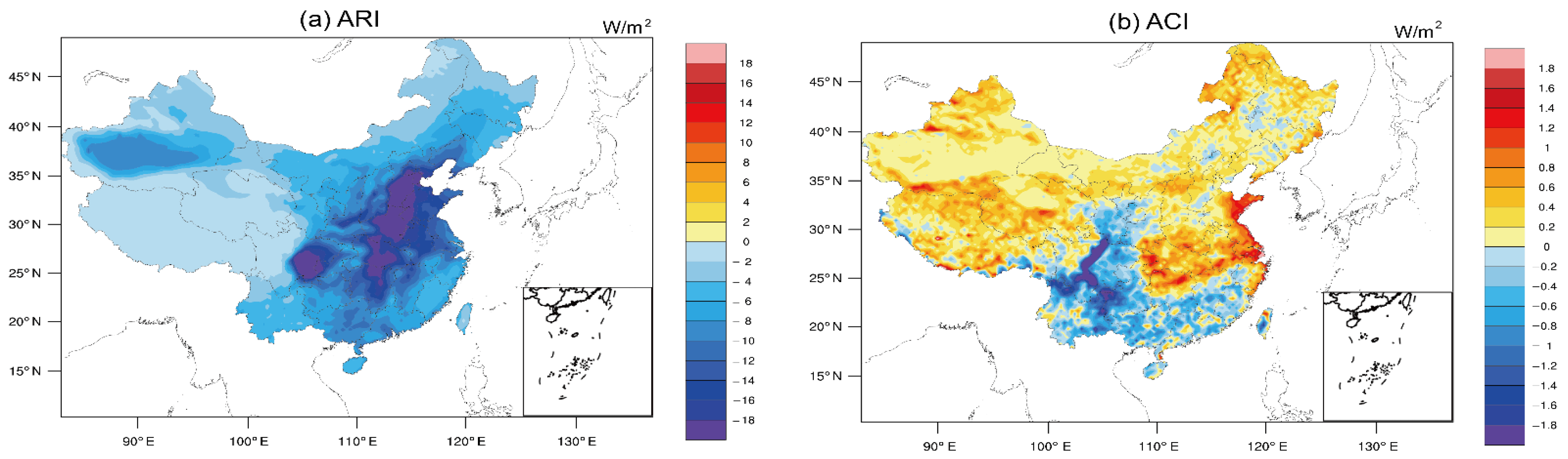
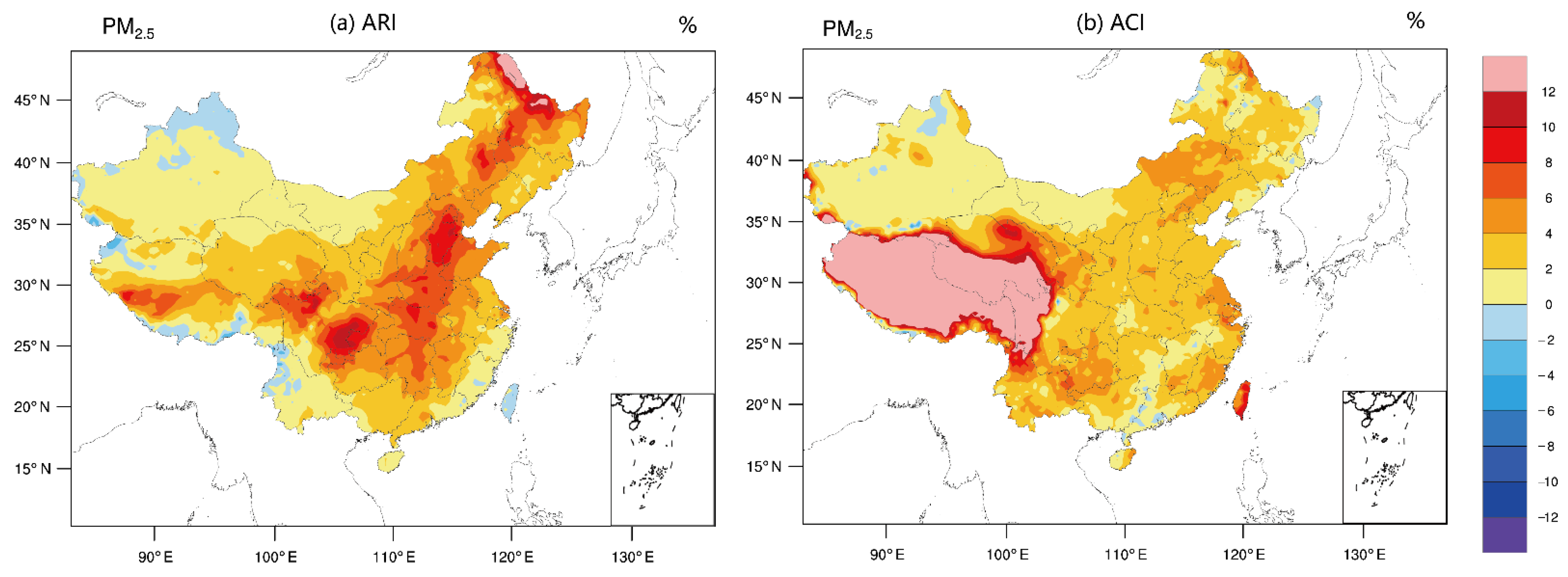
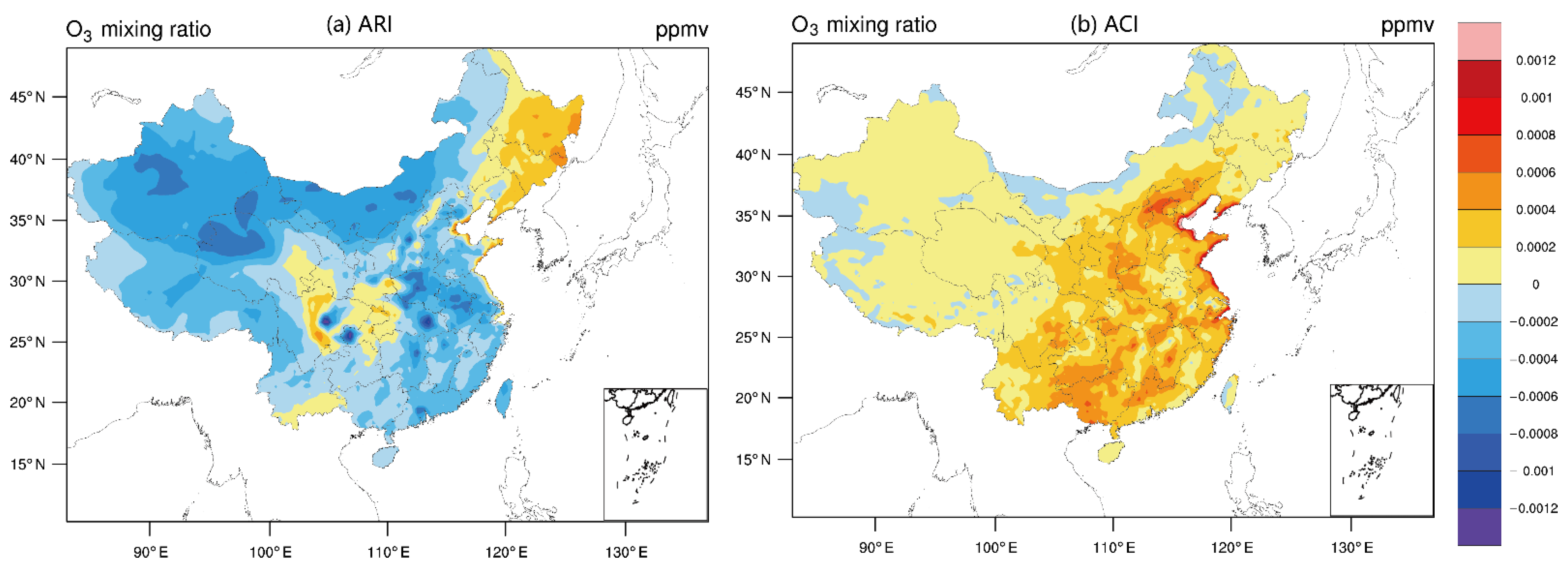
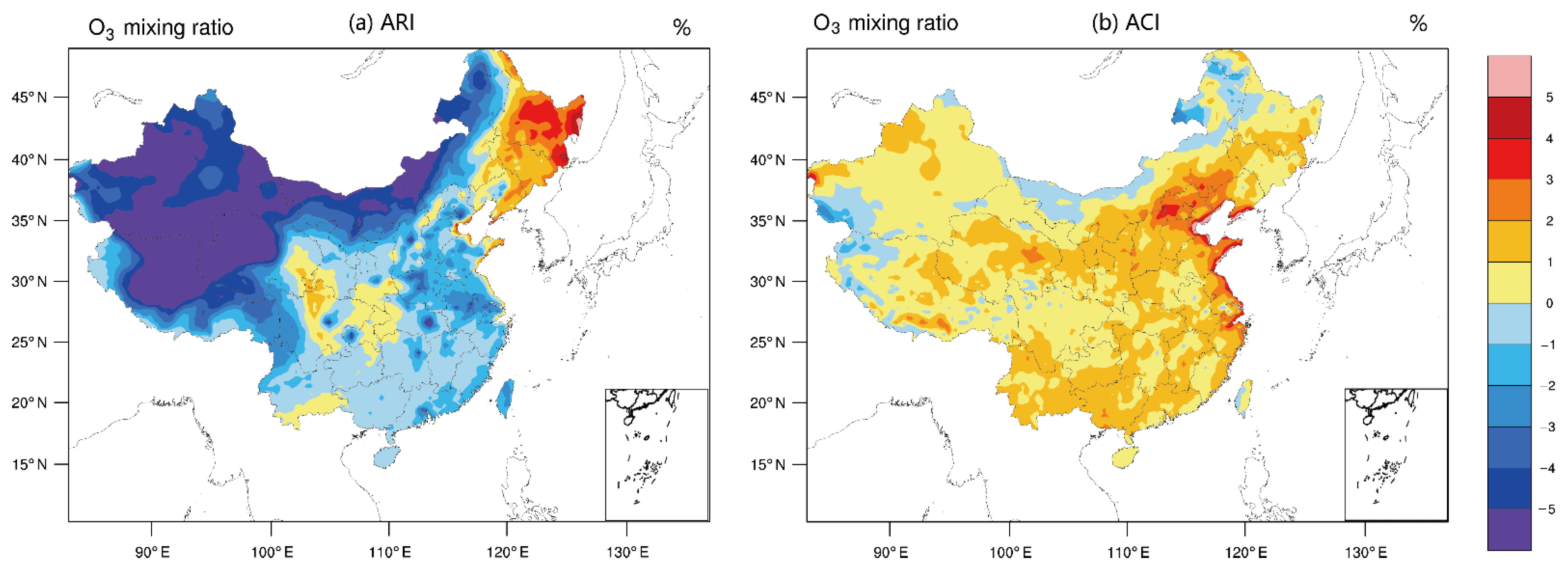
3.2. Changes of PM2.5 and Ozone Concentration due to ARIs and ACIs

The results of the absolute change in the concentrations of PM2.5 are presented in panels A and B of Figure 9, while the percentages of the relative change are shown in Figure 10. The figure shows that northern China and central China as well as the Sichuan Basin experienced a significant increase of the annual mean concentrations of PM2.5 due to ARIs. The maximum annual mean enhancement of mass concentration reached over 12 μg/m3, with an over 10% rise being observed in the scenario without any aerosol–meteorology feedback. Regarding ACIs, the extent of the positive changes observed in the PM2.5 mass concentration was relatively lower, with the annual maximum mean value reaching around 4 μg/m3. The relative change in the PM2.5 concentration ranged from approximately 4 to 6% in most parts of mainland China. However, the maximum percentage of change due to ACIs was found in the Tibet Plateau, where the background is overly clean. In summary, the figures show the differences between the effectiveness in year-round enhancement due to ARIs and ACIs. Specifically, the impact of ARIs in the local aggregation of the PM2.5 concentrations is more significant than the changes seen that were caused by ACIs. Moreover, the spatial distribution indicates a more significant enhancement where the PM2.5 concentrations are higher, suggesting a nonlinear relationship. This is consistent with previous studies [27,28].
Concerning ozone, there is a profound variance observed in Figure 11 and Figure 12. ARIs can reduce ozone in the majority of mainland China, where the PM2.5 enhancement feedback is relatively high. The maximum declines of over 1 ppbv annually are located in the metropolises. This drop is approximately 4% and is mainly observed in very large cities in regions such as Chengdu, Chongqing, Wuhan, Zhengzhou, and some surrounding satellite cities. The reduced short-wavelength radiation that is received on the surface yields a smaller ozone concentration than the ones produced in the corresponding regions. This trend can be identified in Figure 5. However, when it comes to ozone variation due to ACIs, most of the changes are positive. The maximum increases are along the seashore due to the land–sea breeze that transports ozone. Urban and rural differences in the spatial distribution of ozone do not exist in this panel figure. PM-polluted areas display only a 1–2% increase in ozone pollution. This increase is averaged annually, and it may result from the combined contribution of increased shortwave radiation and decreased relative humidity. From the figures that are shown below, we can see a clear divide along the south bank of the Yangtze River. The northern part receives more shortwave radiation due to the ACIs, which improve ozone production, while the southern part experiences an atmosphere that is drier by about −0.2% annually. Lower relative humidity and stronger solar radiation both enhance ozone pollution.

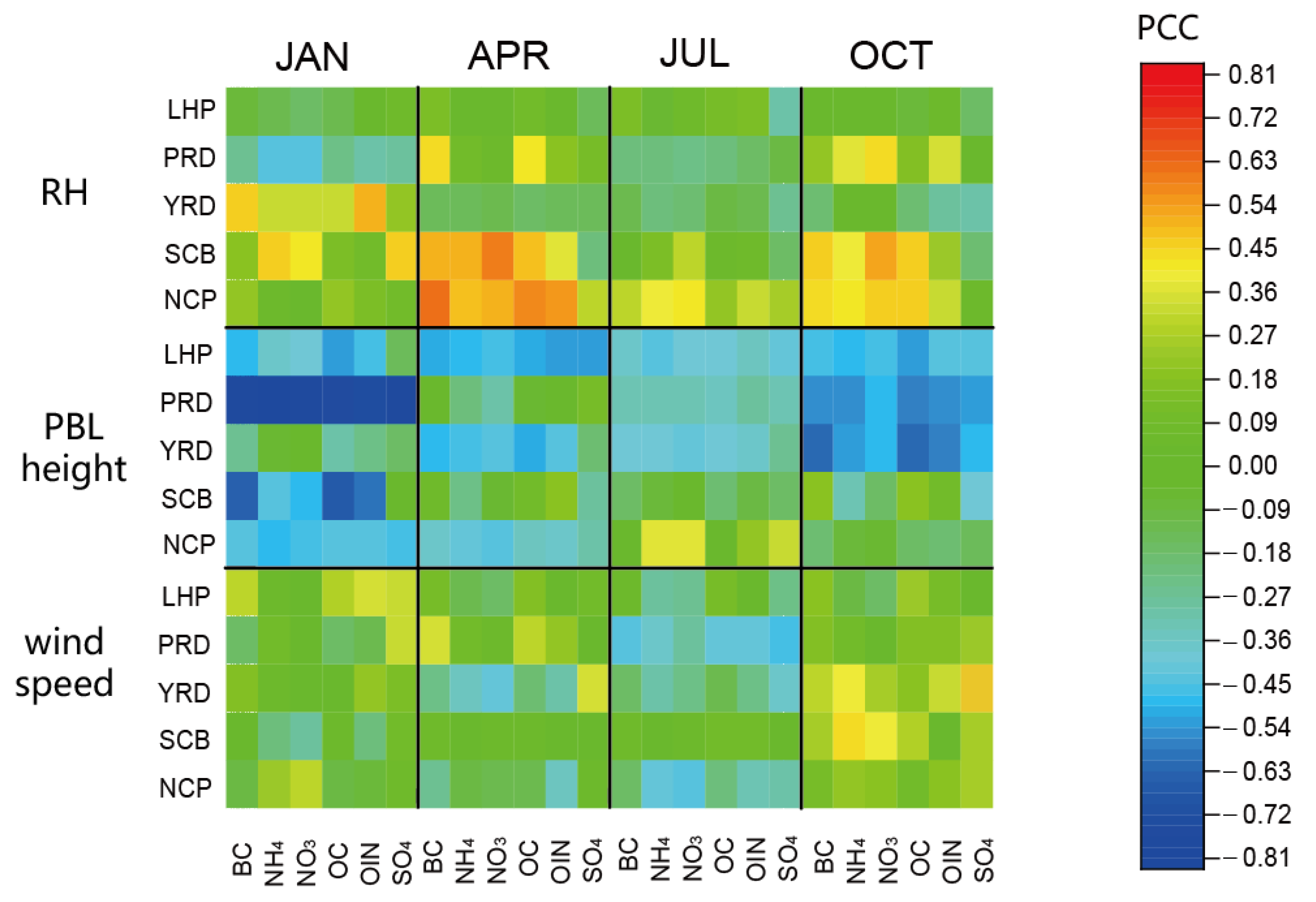
3.3. Partial Correlation Coefficient Analysis
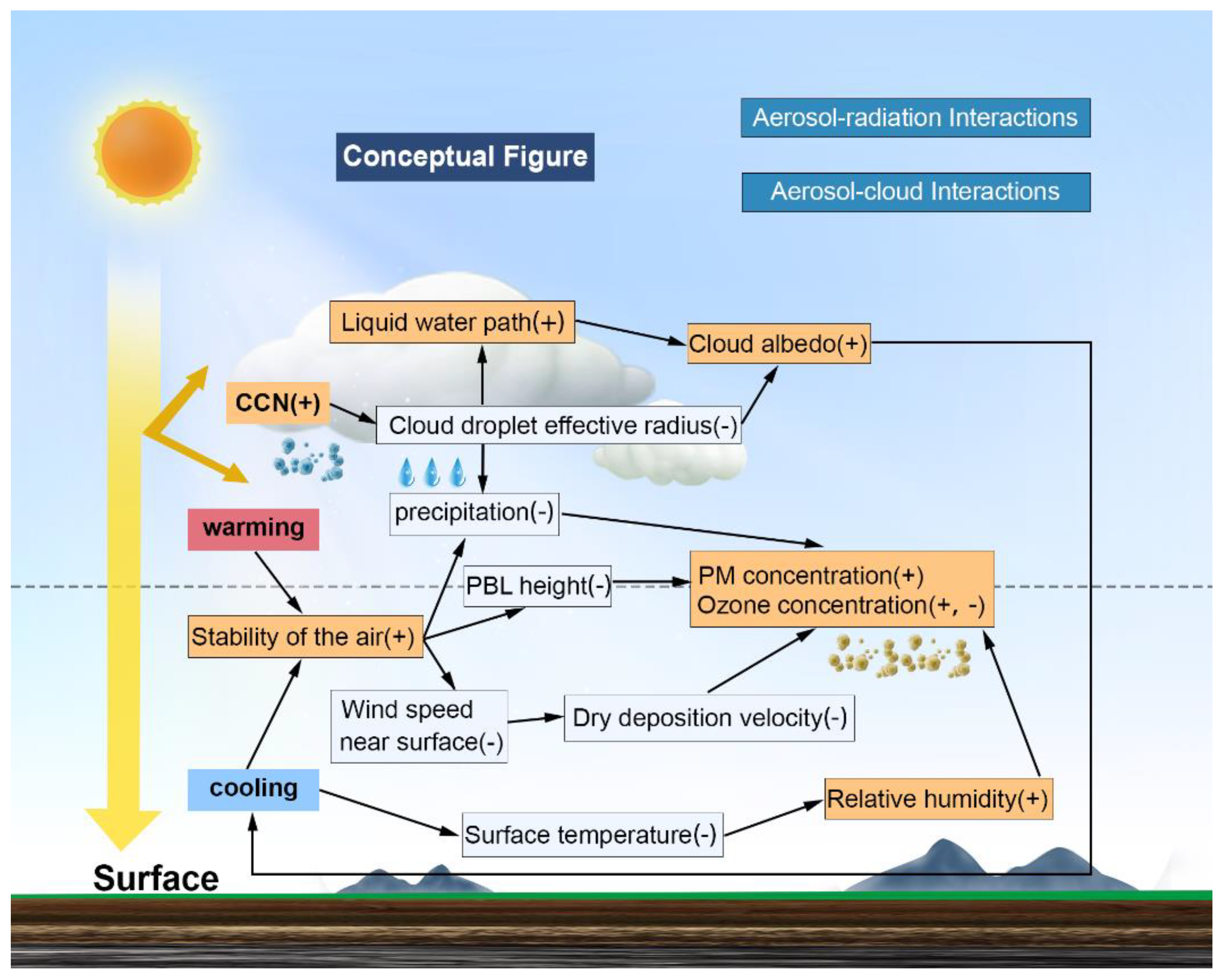
Connections between the different factors and the relative contributions of these factors have yet to be quantified. In order to assess these factors in depth, the partial correlation coefficient (PCC) of these parameters was calculated by season, particle elements, and weather conditions. PCC measures the linear dependence of a pair of variables from a set of variable collections when the influence of the other variables is ruled out. Therefore, it is suitable for analyzing sophisticated systems such as the one discussed here.
In the following equation, r y x . z represents the cofactor in the determinant of the matrix of the variables of the empirical correlation coefficients.
r y x . z = r y x ( r y z ) ( r x z ) 1 r y z 2 1 r x z 2
From the equation, the partial correlation coefficient can be calculated. The significance of correlation can be examined by Student’s t-test, with certain degrees of freedom depending on the size of the dataset. In this circumstance, variables are averaged in daily mean values. Therefore, the degrees of freedom for the test on Student’s t distribution vary from month to month due to the different number of days in each month. Moreover, the elements of different particles are separated for presenting in-depth feedback of PCC in different seasons. The five typical regions, as mentioned above, are also listed on the left vertical axis of Figure 13. For the elements of fine particles, there are six categories listed, including black carbon (BC), ammonia (NH4), nitrate (NO3), organic carbon (OC), other inorganics (OIN), and sulfate (SO4). Meteorological factors include relative humidity (RH), PBL height, and wind speed. Herein, the colors in different boxes indicate PCC values of elements and meteorological factors in the corresponding month and region. As mentioned above, Student’s t-test is performed to ensure the significance of the statistical correlation between variables by checking the r value. The PCC with green color indicates that it is not statistically significant for the correlation, while red and blue boxes suggest positive and negative correlation coefficients with statistical significance.
As demonstrated in the figure, the PBL height is negatively correlated with all six species of PM2.5 in nearly all five regions throughout the year. The season with the most significant correlation when PBL height is crucial to PM species is winter, followed by autumn. As for RH, the largest positive correlation coefficient lies in the spring, when most species such as nitrate and ammonia are positively correlated with RH. The finding is consistent with the conclusion drawn by Wang Xuan et al., who proposed that the measured hygroscopic growth of nitrate and ammonia was stronger than sulfate in a pollution episode in Beijing [44]. Wind speed shows a negative association in summer and a positive correlation with certain species in autumn, accounting for the chemical transfer from higher to lower polluted areas, particularly when cold fronts are active during the transition period between two seasons. For instance, both the ammonia in the Sichuan Basin and sulfate in the Yangtze River Delta positively correlate with wind speed in autumn. In other words, the species show an upward trend when the wind blows harder. Given the prevailing southward wind in autumn, corresponding species can be transferred to the south of China, which can explain the positive partial correlation coefficient of wind speed for certain species in autumn.
PCC is also calculated upon comparison with the mass concentration of PM2.5 in different areas. It is worth noting that all of the PCC values that meet the threshold are shown, and others are marked with crosses in the table. According to the results, wind speed is only insignificantly correlated with PM enhancement due to feedback in most regions during most months except for July in PRD. It is assumed that this negative correlation results from the seasonal movement of the subtropical high in summer. PBL height is negatively correlated with the particle concentration to the most significant extent, particularly in January and October, when three out of five regions show a significantly negative correlation with PBL height, the coefficients of which are significant at the 0.01 level. In terms of aerosol–radiation feedback, shortwave radiation at ground level reduces due to thick aerosol loading. Consequently, the development of PBL is inhibited, which is consistent with these negative PCCs in Table 5. In other words, aerosol can lead to shallower PBL and the local aggregation of aerosols. Relative humidity is another factor changing the concentration of PM2.5 in some regions through hygroscopic growth and the potential chemical productions on the surface of aerosols. The PCC of RH is also shown in the table. It can be seen from this table that the PCCs of RH only show statistical significance during April in North China Plain and Sichuan Basin. The strong positive correlation in the specific region and time provides evidence for the significance of hygroscopic growth in wetter months through aerosol feedback.
The correlation coefficients of ozone were also calculated for the five representative regions. The coefficients with statistical significance (p < 0.01) are listed in Table 6. The coefficients indicate the relationship between the atmospheric variables and the absolute change in ozone concentration due to ACIs. More variables are factored into the statistical analysis to further verify the potential association between the variables and ozone pollution, with chemical variables such as NO2 and meteorological variables such as temperature, humidity, PBL height, and shortwave radiation received the surface. Those with no significance are indicated by a cross in the corresponding box.
There is a substantial difference between regions in terms of the significance shown by correlation coefficients. In NCP, the most significant ones include relative humidity and temperature, where relatively drier and hotter air can cause heavier ozone pollution through ACI processes. In the Sichuan Basin, significant coefficients include NO2 and nitrate oxidation ratio (NOR). Within the two city clusters along the middle and lower reaches of the Yangtze River, LHP and YRD suffered the most significant impact from NO2 concentration followed by the received radiation and sulfur oxidation ratio (SOR) due to ACIs, which may be attributed to the involvement of cloud nuclei in cloud microphysics across these two regions. For PRD, none of the variables has passed the hypothesized Student’s t-test. Thus, only the cross is shown in the column.

4. Discussion

Based on the previous discussion, a conceptual figure is shown in Figure 14. The pathways for ARIs and ACIs are illustrated by detailed steps. Some chemical contributors are not included in the figure owing to the limited size of the figure. Considering ARIs and ACIs, the reduction of surface wind along with increased relative humidity is contributory to the enhancement of PM2.5 concentration. However, ozone change varies partly due to the negative correlation with relative humidity. Other chemical factors are also vitally important to the ozone concentration, evidence of which is provided in Table 6.
Within the processes of ARIs, the surface can be cooled down due to the scattering and absorbing characteristics of aerosols. Surface temperature is thus reduced, as indicated in Figure 5a and Figure 6a. Declining air temperature on the surface is conducive to the increase of local relative humidity (Figure 6c) via the decrease of saturated water vapor pressure. On the other hand, lower air temperature on the surface can result in temperature inversion, enhancing the stability of atmosphere within the boundary layer. Therefore, the development of the planetary boundary layer is suppressed (Figure 7a). On the other hand, wind speed near the surface (Figure 8a) and the dry deposition velocity of particles are also reduced, which is similar to the findings from the previous study [43].
In addition, ACIs can be vital to the change of the meteorological factors. Cooler surface (Figure 6b), higher relative humidity (Figure 6d), shallower PBL (Figure 7b), and slower wind (Figure 8b) can also be found in the majority of mainland China, but to a smaller extent when comparing with the influence by ARIs. The ACI pathways within the WRF-Chem model have been referred to in previous studies [23,43], which presented cloud microphysics in the calculation in depth.
As a result, the concentration of PM2.5 is mounting in the corresponding regions (Figure 9a,b and Figure 10a,b) via both ARIs and ACIs. In terms of ozone, the influences can be found especially in urban regions in central and eastern China, which can be attributed to the reduced radiation as well as the changed NO2 mixing ratio (Figure S5) along with increased relative humidity.
Due to the limits on time and computer resources, some issues are left unsolved. Previous studies revealed the importance of heterogeneous reactions to the chemical transport model [45,46,47], leading to a significant improvement of model performance in quantifying pollutants. However, in this study, these reactions were not included, resulting in some uncertainties. In addition, the simulation only covers four months. Since all-year-round simulation is computationally expensive, it was not considered in the study. In a case where adequate computing resources, an all-year simulation is recommended to obtain more accurate results for identifying the influences of feedback. Moreover, the options in cloud microphysics are also contributory to the uncertainties of the role of ACIs in the feedback [48,49,50,51]. It is thus necessary to conduct further studies with upgraded sophisticated model configuration for the continued validation of the relevant scientific mechanisms. It is also recommended that the simulation tools continue to undergo development in the future In order for them to continue to present reliable temporal and spatial distribution with smaller biases. This not only refers to a regional atmospheric chemistry transport model such as the WRF-Chem model but also to global models [52,53,54,55,56,57,58], which are conducive to the elucidation of air pollution issues on different scales. Special attention should be paid to the long transportation time between polluted regions as well as the constraints in uncertainties of land–atmosphere interactions [59,60,61].

5. Conclusions

To better understand the intricate impacts of aerosol–meteorology interactions on PM2.5 and ozone concentration, the up-to-date, sophisticated atmospheric chemistry model WRF-Chem was applied while ensuring that the sensitivity tests were conducted with the proper settings applied. These tests can help distinguish between the influence of ARIs and that of ACIs. According to the results, the positive feedback increased PM2.5 concentration through both ARIs and ACIs. However, the extent of the influence is more significant in ARIs than it is in ACIs. As for ozone pollution, ARIs can reduce the level by 4%, while ACIs can alleviate the increase in pollution by roughly 1 ppbv. As for the spatial distribution of the changes in ozone, it also varies between ARIs and ACIs. Significant ozone reduction via ARIs was found in the surrounding areas of the inland metropolises, while more significant changes via ACIs were found along the coastline due to transportation by the land–sea breeze.
The partial correlation coefficients of PM2.5 and ozone concentrations were analyzed using the variables in those representative city clusters across China, and a discussion about different seasons and chemical species was detailed. The impact of PBL height plays the most important role in causing changes to PM2.5 concentration, followed by relative humidity, which is due to the hygroscopic growth process. The most significant variable for ozone is NO2 followed by solar radiation density and oxidation rates, which provide a reference for future investigation into the mechanism of joint control on PM2.5 and ozone pollution in China, especially considering the feedback of the aerosol–meteorology interactions.

Supplementary Materials

The following are available online at https://0-www-mdpi-com.brum.beds.ac.uk/article/10.3390/atmos12121585/s1, Figure S1: Temporal trend of simulated and observed air temperature (°C) at 2 meter level in different regions in January, April, July, and October. Figure S2: Temporal trend of simulated and observed relative humidity (%) at 2 meter level in different regions in January, April, July, and October. Figure S3: Temporal trend of simulated and observed wind speed (m/s) at 10 meter level in different regions in January, April, July, and October. Figure S4: The spatial distribution of mean bias of precipitation in different months (unit: mm). Figure S5: Change of NO2 due to different feedbacks in different months (unit: ppmv).

Author Contributions

Conceptualization, X.Z.; methodology, X.Z.; software, X.Z.; validation, X.Z., and C.Y.; formal analysis, X.Z.; investigation, X.Z; resources, X.Z.; data curation, X.Z.; writing—original draft preparation, X.Z. and C.Y.; writing-review and editing, X.Z., C.Y. and Z.Z.; visualization, X.Z., C.Y. and Z.Z.; supervision, X.Z.; project administration, X.Z.; funding acquisition, X.Z. All authors have read and agreed to the published version of the manuscript.

Funding

The research is supported by the Fundamental Research Funds for the Central Universities (3122019066) and Scientific Initiation Funds of CAUC (2020KYQD119).

Institutional Review Board Statement

Not applicable.

Informed Consent Statement

Not applicable.

Data Availability Statement

Data are available upon request.

Acknowledgments

The authors acknowledge the model group for the effort in supporting WRF-Chem users. Additionally, the authors thank the staff from NECI and CNEMC for providing the high-quality dataset. Thanks are given to the National Super Computer Center in Tianjin, China, for providing the computational platform.

Conflicts of Interest

The authors declare no conflict of interest.

Appendix A

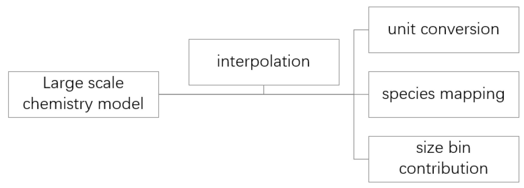
Explanation of the Calculation in the WRF-Chem Model Regarding the Meteorological Factors and Chemical Species

The calculations within WRF-Chem can be classified into two major categories, i.e., meteorological parts and chemical species.
Meteorology:
We used NCAR final analysis data as the input meteorological data. After ungrib and interpolate processes into the grids of WRF-Chem, the data can be used as the model’s initial and boundary conditions. The steps for preprocessing section are shown in the figure below (Figure A1).
Figure A1. Meteorological preprocessing steps in WRF model.
Atmosphere 12 01585 g0a1
Chemistry:
The chemistry portion is triggered by linking the natural emissions, anthropogenic emissions, and chemical boundary conditions from Mozart (Figure A2), which can be downloaded from the WRF-Chem official website by customizing the specific date, time duration, and region coordinates. The conversion from different scales of emission inventories and chemical boundary conditions must undergo these procedures. Detailed choice of both anthropogenic and natural emission inventory can be seen in the Chapter 2.1 section.
Figure A2. Usage of the chemical input data in providing chemical boundary conditions.
Atmosphere 12 01585 g0a2
The overall procedures are shown in the Figure below (Figure A3). This figure is open-access to the public by the official website of WRF-Chem model.
Figure A3. WRF-Chem model flow chart (Source: https://ruc.noaa.gov/wrf/wrf-chem/wrf_tutorial_2015/WRF_CHEM_setup.pdf, accessed on 11 November, 2021).
Atmosphere 12 01585 g0a3
In our study, the input emissions were the MEGAN natural emission inventory, the MEIC emission inventory for China, the MOZART chemical model for the chemical boundaries, and the NCEP/NCAR final analysis data as the initial meteorological and boundary conditions.
The programming language and software we used in the study for post-possessing and visualization were python, NCL (NCAR Command Language), and the Origin software.
Interactions between the meteorological and chemical parts were dealt with in the details of each of the modules in the state-of-the-art model. The interactions from the cloud microphysics and aqueous phase chemistry can interact with aerosol microphysics in the corresponding module, thus modifying the outcome. The explanation can be found in Figure A4.
Figure A4. Interactions with different modules in the WRF-Chem model in the simulation (Source: https://ruc.noaa.gov/wrf/wrf-chem/wrf_tutorial_2015/WRF_CHEM_aerosols.pdf, accessed on 11 November 2021).
Atmosphere 12 01585 g0a4
Based on the structure of the model, following designs of numerical experiments are implemented. When carrying out three sets of parallel sensitivity tests as indicated in the manuscript, we conducted the modifications in either the namelist configuration or the codes in the corresponding modules of cloud microphysics. The relative contribution of the aerosol–radiation interaction (ARIs) and aerosol–cloud interactions (ACIs) was therefore determined by comparing the differences of the results. The configuration of the parallel sensitivity tests is listed in Table 2 in the main content of the manuscript.

References

  1. Yang, K.; Kong, L.; Tong, S.; Shen, J.; Chen, L.; Jin, S.; Wang, C.; Sha, F.; Wang, L. Double High-Level Ozone and PM2.5 Co-Pollution Episodes in Shanghai, China: Pollution Characteristics and Significant Role of Daytime HONO. Atmosphere 2021, 12, 557. [Google Scholar] [CrossRef]
  2. Shu, L.; Wang, T.; Xie, M.; Li, M.; Zhao, M.; Zhang, M.; Zhao, X. Episode study of fine particle and ozone during the CAPUM-YRD over Yangtze River Delta of China: Characteristics and source attribution. Atmos. Environ. 2019, 203, 87–101. [Google Scholar] [CrossRef]
  3. Xing, J.; Wang, S.X.; Jang, C.; Zhu, Y.; Hao, J.M. Nonlinear response of ozone to precursor emission changes in China: A modeling study using response surface methodology. Atmos. Chem. Phys. 2011, 11, 5027–5044. [Google Scholar] [CrossRef] [Green Version]
  4. Lu, X.; Hong, J.; Zhang, L.; Cooper, O.R.; Schultz, M.G.; Xu, X.; Wang, T.; Gao, M.; Zhao, Y.; Zhang, Y. Severe Surface Ozone Pollution in China: A Global Perspective. Environ. Sci. Technol. Lett. 2018, 5, 487–494. [Google Scholar] [CrossRef]
  5. Zheng, B.; Tong, D.; Li, M.; Liu, F.; Hong, C.; Geng, G.; Li, H.; Li, X.; Peng, L.; Qi, J.; et al. Trends in China’s anthropogenic emissions since 2010 as the consequence of clean air actions. Atmos. Chem. Phys. 2018, 18, 14095–14111. [Google Scholar] [CrossRef] [Green Version]
  6. Zhang, Q.; Zheng, Y.; Tong, D.; Shao, M.; Wang, S.; Zhang, Y.; Xu, X.; Wang, J.; He, H.; Liu, W.; et al. Drivers of improved PM2.5 air quality in China from 2013 to 2017. Proc. Natl. Acad. Sci. USA 2019, 116, 24463–24469. [Google Scholar] [CrossRef] [Green Version]
  7. Li, K.; Chen, L.; Ying, F.; White, S.J.; Jang, C.; Wu, X.; Gao, X.; Hong, S.; Shen, J.; Azzi, M.; et al. Meteorological and chemical impacts on ozone formation: A case study in Hangzhou, China. Atmos. Res. 2017, 196, 40–52. [Google Scholar] [CrossRef]
  8. Zhao, S.; Wang, L.; QI, M.; Lu, X.; Wang, Y.; Liu, Z.; Liu, Y.; Tan, J.; Zhang, Y.; Wang, Q.; et al. Study on the characteristics and mutual influence of PM2.5-O3 complex pollution in Handan. Acta Sicentiae Circumstantiae 2021, 41, 2250–2261. [Google Scholar]
  9. Benas, N.; Mourtzanou, E.; Kouvarakis, G.; Bais, A.; Mihalopoulos, N.; Vardavas, I. Surface ozone photolysis rate trends in the Eastern Mediterranean: Modeling the effects of aerosols and total column ozone based on Terra MODIS data. Atmos. Environ. 2013, 74, 1–9. [Google Scholar] [CrossRef]
  10. Jia, M.; Zhao, T.; Cheng, X.; Gong, S.; Zhang, X.; Tang, L.; Liu, D.; Wu, X.; Wang, L.; Chen, Y. Inverse Relations of PM2.5 and O3 in Air Compound Pollution between Cold and Hot Seasons over an Urban Area of East China. Atmosphere 2017, 8, 59. [Google Scholar] [CrossRef] [Green Version]
  11. Zhu, J.; Chen, L.; Liao, H.; Dang, R. Correlations between PM2.5 and Ozone over China and Associated Underlying Reasons. Atmosphere 2019, 10, 352. [Google Scholar] [CrossRef] [Green Version]
  12. Li, K.; Jacob, D.J.; Liao, H.; Shen, L.; Zhang, Q.; Bates, K.H. Anthropogenic drivers of 2013–2017 trends in summer surface ozone in China. Proc. Natl. Acad. Sci. USA 2019, 116, 422–427. [Google Scholar] [CrossRef] [PubMed] [Green Version]
  13. Tan, Z.; Fuchs, H.; Lu, K.; Bohn, B.; Broch, S.; Dong, H.; Gomm, S.; Haeseler, R.; He, L.; Hofzumahaus, A.; et al. Radical chemistry at a rural site (Wangdu) in the North China Plain: Observation and model calculations of OH, HO2 and RO2 radicals. Atmos. Chem. Phys. 2017, 17, 4453. [Google Scholar] [CrossRef] [Green Version]
  14. Wang, B. A novel causality-centrality-based method for the analysis of the impacts of air pollutants on PM2.5 concentrations in China. Sci. Rep. 2021, 11, 6960. [Google Scholar] [CrossRef] [PubMed]
  15. Yahya, K.; Wang, K.; Zhang, Y.; Kleindienst, T. Application of WRF/Chem over North America under the AQMEII Phase 2–Part 2: Evaluation of 2010 application and responses of air quality and meteorology–chemistry interactions to changes in emissions and meteorology from 2006 to 2010. Geosci. Model. Dev. 2015, 8, 2095–2117. [Google Scholar] [CrossRef] [Green Version]
  16. Kong, X.; Forkel, R.; Sokhi, R.S.; Suppan, P.; Baklanov, A.; Gauss, M.; Brunner, D.; Barò, R.; Balzarini, A.; Chemel, C. Analysis of meteorology–chemistry interactions during air pollution episodes using online coupled models within AQMEII phase-2. Atmos. Environ. 2015, 115, 527–540. [Google Scholar] [CrossRef]
  17. Gao, Y.; Zhang, M.; Liu, Z.; Wang, L.; Wang, P.; Xia, X.; Tao, M.; Zhu, L. Modeling the feedback between aerosol and meteorological variables in the atmospheric boundary layer during a severe fog–haze event over the North China Plain. Atmos. Chem. Phys. 2015, 15, 4279–4295. [Google Scholar] [CrossRef] [Green Version]
  18. Wang, J.; Wang, S.; Jiang, J.; Ding, A.; Zheng, M.; Zhao, B.; Wong, D.C.; Zhou, W.; Zheng, G.; Wang, L. Impact of aerosol–meteorology interactions on fine particle pollution during China’s severe haze episode in January 2013. Environ. Res. Lett. 2014, 9, 094002. [Google Scholar] [CrossRef]
  19. Zhang, B.; Wang, Y.; Hao, J. Simulating aerosol–radiation–cloud feedbacks on meteorology and air quality over eastern China under severe haze conditionsin winter. Atmos. Chem. Phys. 2015, 15, 2387–2404. [Google Scholar] [CrossRef] [Green Version]
  20. Gao, M.; Carmichael, G.R.; Wang, Y.; Saide, P.; Yu, M.; Xin, J.; Liu, Z.; Wang, Z. Modeling study of the 2010 regional haze event in the North China Plain. Atmos. Chem. Phys. 2016, 16, 1673–1691. [Google Scholar] [CrossRef] [Green Version]
  21. Petäjä, T.; Järvi, L.; Kerminen, V.-M.; Ding, A.; Sun, J.; Nie, W.; Kujansuu, J.; Virkkula, A.; Yang, X.; Fu, C. Enhanced air pollution via aerosol-boundary layer feedback in China. Sci. Rep. 2016, 6, 18998. [Google Scholar] [CrossRef] [Green Version]
  22. Tie, X.; Huang, R.J.; Cao, J.; Zhang, Q.; Cheng, Y.; Su, H.; Chang, D.; Poschl, U.; Hoffmann, T.; Dusek, U.; et al. Severe Pollution in China Amplified by Atmospheric Moisture. Sci. Rep. 2017, 7, 15760. [Google Scholar] [CrossRef]
  23. Zhao, B.; Liou, K.N.; Gu, Y.; Li, Q.; Jiang, J.H.; Su, H.; He, C.; Tseng, H.R.; Wang, S.; Liu, R.; et al. Enhanced PM2.5 pollution in China due to aerosol-cloud interactions. Sci. Rep. 2017, 7, 4453. [Google Scholar] [CrossRef] [Green Version]
  24. Gao, Y.; Zhao, C.; Liu, X.; Zhang, M.; Leung, L.R. WRF-Chem simulations of aerosols and anthropogenic aerosol radiative forcing in East Asia. Atmos. Environ. 2014, 92, 250–266. [Google Scholar] [CrossRef]
  25. Forkel, R.; Balzarini, A.; Baró, R.; Bianconi, R.; Curci, G.; Jiménez-Guerrero, P.; Hirtl, M.; Honzak, L.; Lorenz, C.; Im, U. Analysis of the WRF-Chem contributions to AQMEII phase2 with respect to aerosol radiative feedbacks on meteorology and pollutant distributions. Atmos. Environ. 2015, 115, 630–645. [Google Scholar] [CrossRef]
  26. Chen, D.-S.; Ma, X.; Xie, X.; Wei, P.; Wen, W.; Xu, T.; Yang, N.; Gao, Q.; Shi, H.; Guo, X. Modelling the effect of aerosol feedbacks on the regional meteorology factors over China. Aerosol. Air. Qual. Res. 2015, 15, 1559–1579. [Google Scholar] [CrossRef] [Green Version]
  27. Zhou, M.; Zhang, L.; Chen, D.; Gu, Y.; Fu, T.-M.; Gao, M.; Zhao, Y.; Lu, X.; Zhao, B. The impact of aerosol–radiation interactions on the effectiveness of emission control measures. Environ. Res. Lett. 2019, 14, 024002. [Google Scholar] [CrossRef]
  28. Peng, Y.; Zhang, X.; Zhang, Q. Impact of the implementation of the “Ten Statements of Atmosphere” on the atmospheric aerosol-radiation interaction during 2013–2017. Acta Sicentiae Circumstantiae 2021, 41, 311–320. [Google Scholar]
  29. Li, M.; Zhang, Q.; Kurokawa, J.-I.; Woo, J.; He, K.; Lu, Z.; Ohara, T.; Song, Y.; Streets, D.; Carmichael, G. MIX: A mosaic Asian anthropogenic emission inventory for the MICS-Asia and the HTAP projects. Atmos. Chem. Phys. Discuss. 2015, 15, 34813–34869. [Google Scholar]
  30. Guenther, A.; Karl, T.; Harley, P.; Wiedinmyer, C.; Palmer, P.I.; Geron, C. Estimates of global terrestrial isoprene emissions using MEGAN (Model of Emissions of Gases and Aerosols from Nature). Atmos. Chem. Phys. 2006, 6, 3181–3210. [Google Scholar] [CrossRef] [Green Version]
  31. Iacono, M.J.; Delamere, J.S.; Mlawer, E.J.; Shephard, M.W.; Clough, S.A.; Collins, W.D. Radiative forcing by long-lived greenhouse gases: Calculations with the AER radiative transfer models. J. Geophys. Res. Atmos. 2008, 113, D13103. [Google Scholar] [CrossRef]
  32. Gettelman, A.; Morrison, H. A New Two-Moment Bulk Stratiform Cloud Microphysics Scheme in the Community Atmosphere Model, Version 3 (CAM3). Part I: Description and Numerical Tests. J. Clim. 2008, 21, 3642–3659. [Google Scholar] [CrossRef]
  33. Kain, J.S. The Kain–Fritsch convective parameterization: An update. J. Appl. Meteorol. Climatol. 2004, 43, 170–181. [Google Scholar] [CrossRef] [Green Version]
  34. Jiménez, P.A.; Dudhia, J. On the ability of the WRF model to reproduce the surface wind direction over complex terrain. J. Appl. Meteorol. Climatol. 2013, 52, 1610–1617. [Google Scholar] [CrossRef]
  35. Foken, T. 50 years of the Monin–Obukhov similarity theory. Bound. Layer Meteorol. 2006, 119, 431–447. [Google Scholar] [CrossRef]
  36. Hong, S.-Y.; Noh, Y.; Dudhia, J. A new vertical diffusion package with an explicit treatment of entrainment processes. Mon. Weather Rev. 2006, 134, 2318–2341. [Google Scholar] [CrossRef] [Green Version]
  37. Wild, O.; Zhu, X.; Prather, M.J. Fast-J: Accurate simulation of in-and below-cloud photolysis in tropospheric chemical models. J. Atmos. Chem. 2000, 37, 245–282. [Google Scholar] [CrossRef]
  38. San José, R.; Pérez, J.; Balzarini, A.; Baró, R.; Curci, G.; Forkel, R.; Galmarini, S.; Grell, G.; Hirtl, M.; Honzak, L. Sensitivity of feedback effects in CBMZ/MOSAIC chemical mechanism. Atmos. Environ. 2015, 115, 646–656. [Google Scholar] [CrossRef] [Green Version]
  39. Makar, P.; Gong, W.; Milbrandt, J.; Hogrefe, C.; Zhang, Y.; Curci, G.; Žabkar, R.; Im, U.; Balzarini, A.; Baró, R. Feedbacks between air pollution and weather, Part 1: Effects on weather. Atmos. Environ. 2015, 115, 442–469. [Google Scholar] [CrossRef]
  40. Makar, P.; Gong, W.; Hogrefe, C.; Zhang, Y.; Curci, G.; Žabkar, R.; Milbrandt, J.; Im, U.; Balzarini, A.; Baró, R. Feedbacks between air pollution and weather, Part 2: Effects on chemistry. Atmos. Environ. 2015, 115, 499–526. [Google Scholar] [CrossRef]
  41. Wang, L.; Zhang, Y.; Wang, K.; Zheng, B.; Zhang, Q.; Wei, W. Application of Weather Research and Forecasting Model with Chemistry (WRF/Chem) over northern China: Sensitivity study, comparative evaluation, and policy implications. Atmos. Environ. 2016, 124, 337–350. [Google Scholar] [CrossRef] [Green Version]
  42. Tao, X.; Huang, J.; Xie, X.; Wang, Y.; Bao, Y.; Liu, C.; Zhang, X.; Xu, J. Observational Analysis of the Influence of Aerosol Radiation Effect on Planetary Boundary Layer Structure and Entrainment Characteristics. Chin. J. Atmos. Sci. 2020, 44, 1213–1233. [Google Scholar]
  43. Zhang, X.; Zhang, Q.; Hong, C.; Zheng, Y.; Geng, G.; Tong, D.; Zhang, Y.; Zhang, X. Enhancement of PM2.5 Concentrations by Aerosol-Meteorology Interactions over China. J. Geophys. Res. Atmos. 2018, 123, 1179–1194. [Google Scholar] [CrossRef]
  44. Wang, X.; Shen, X.J.; Sun, J.Y.; Zhang, X.Y.; Wang, Y.Q.; Zhang, Y.M.; Wang, P.; Xia, C.; Qi, X.F.; Zhong, J.T. Size-resolved hygroscopic behavior of atmospheric aerosols during heavy aerosol pollution episodes in Beijing in December 2016. Atmos. Environ. 2018, 194, 188–197. [Google Scholar] [CrossRef]
  45. Gao, M.; Carmichael, G.R.; Wang, Y.; Ji, D.; Liu, Z.; Wang, Z. Improving simulations of sulfate aerosols during winter haze over Northern China: The impacts of heterogeneous oxidation by NO2. Front. Environ. Sci. Eng. 2016, 10, 1–11. [Google Scholar] [CrossRef]
  46. Archernicholls, S. Evaluated Developments in the WRF-Chem Model; Comparison with Observations and Evaluation of Impacts. Ph.D. Thesis, University of Manchester, Manchester, UK, 2014. [Google Scholar]
  47. Dong, X.; Fu, J.S. Understanding interannual variations of biomass burning from Peninsular Southeast Asia, Part I: Model evaluation and analysis of systematic bias. Atmos. Environ. 2015, 116, 293–307. [Google Scholar] [CrossRef]
  48. Koh, T.Y.; Fonseca, R. Subgrid-scale cloud-radiation feedback for the Betts-Miller-Janji convection scheme. Q. J. R. Meteorol. Soc. 2016, 142, 989–1006. [Google Scholar] [CrossRef] [Green Version]
  49. Zhang, Y.; Zhang, X.; Wang, K.; Zhang, Q.; Duan, F.; He, K. Application of WRF/Chem over East Asia: Part II. Model improvement and sensitivity simulations. Atmos. Environ. 2016, 124, 301–320. [Google Scholar] [CrossRef] [Green Version]
  50. Herwehe, J.A.; Alapaty, K.; Spero, T.L.; Nolte, C.G. Increasing the credibility of regional climate simulations by introducing subgrid-scale cloud-radiation interactions. J. Geophys. Res. Atmos. 2014, 119, 5317–5330. [Google Scholar] [CrossRef]
  51. Sha, T.; Ma, X.; Wang, J.; Tian, R.; Zhao, J.; Cao, F.; Zhang, Y.-L. Improvement of inorganic aerosol component in PM2.5 by constraining aqueous-phase formation of sulfate in cloud with satellite retrievals: WRF-Chem simulations. Sci. Total Environ. 2022, 804, 150229. [Google Scholar] [CrossRef]
  52. Onwukwe, C.; Jackson, P.L. Acid wet-deposition modeling sensitivity to WRF-CMAQ planetary boundary layer schemes and exceedance of critical loads over an industrializing coastal valley in northwestern British Columbia, Canada. Atmos. Pollut. Res. 2021, 12, 231–244. [Google Scholar] [CrossRef]
  53. Ying, Z.; Tie, X.; Li, G. Sensitivity of ozone concentrations to diurnal variations of surface emissions in Mexico City: A WRF/Chem modeling study. Atmos. Environ. 2009, 43, 851–859. [Google Scholar] [CrossRef]
  54. Lei, S.; Xue, L.; Wang, Y.; Li, L.; Wang, W. Impacts of meteorology and emissions on summertime surface ozone increases over central eastern China between 2003 and 2015. Atmos. Chem. Phys. 2019, 19, 1455–1469. [Google Scholar]
  55. Vohra, K.; Vodonos, A.; Schwartz, J.; Marais, E.A.; Mickley, L.J. Global mortality from outdoor fine particle pollution generated by fossil fuel combustion: Results from GEOS-Chem. Environ. Res. 2021, 195, 110754. [Google Scholar] [CrossRef]
  56. Jeong, G.-R. Weather Effects of Aerosols in the Global Forecast Model. Atmosphere 2020, 11, 850. [Google Scholar] [CrossRef]
  57. Schnell, J.L.; Holmes, C.D.; Jangam, A.; Prather, M.J. Skill in forecasting extreme ozone pollution episodes with a global atmospheric chemistry model. Atmos. Chem. Phys. 2014, 14, 7721–7739. [Google Scholar] [CrossRef] [Green Version]
  58. Kang, J.Y.; Bae, S.Y.; Park, R.S.; Han, J.Y. Aerosol indirect effects on the predicted precipitation in a global weather forecasting model. Atmosphere 2019, 10, 392. [Google Scholar] [CrossRef] [Green Version]
  59. Gao, Y.; Chen, F.; Miguez-Macho, G.; Li, X. Understanding precipitation recycling over the Tibetan Plateau using tracer analysis with WRF. Clim. Dyn. 2020, 55, 2921–2937. [Google Scholar] [CrossRef]
  60. Kim, G.; Lee, J.; Lee, M.I.; Kim, D. Impacts of urbanization on atmospheric circulation and aerosol transport in a coastal environment simulated by the WRF-Chem coupled with urban canopy model. Atmos. Environ. 2021, 249, 118253. [Google Scholar] [CrossRef]
  61. da Cunha Luz Barcellos, P.; Cataldi, M. Flash flood and extreme rainfall forecast through one-way coupling of WRF-SMAP models: Natural hazards in Rio de Janeiro state. Atmosphere 2020, 11, 834. [Google Scholar] [CrossRef]
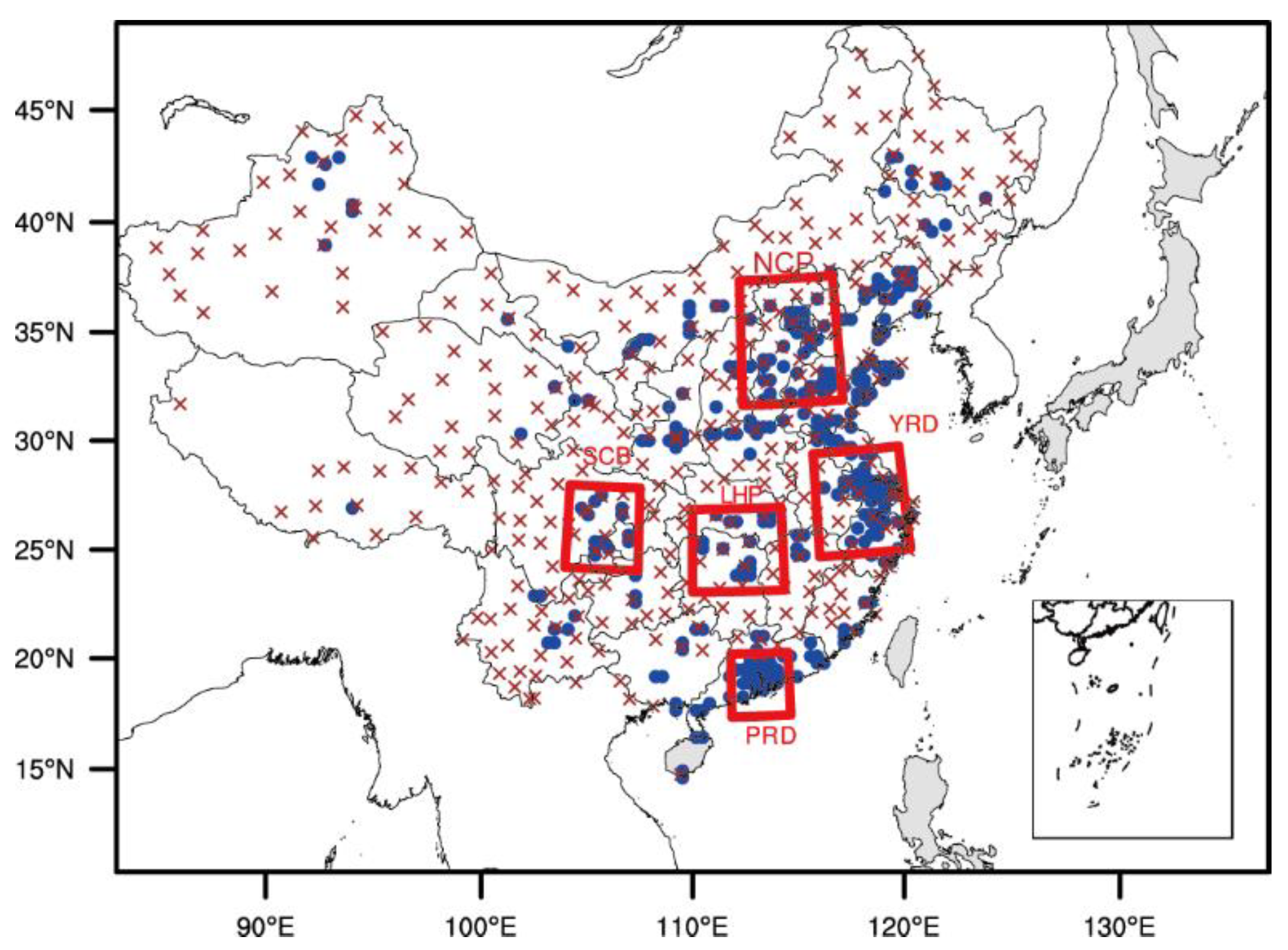
Figure 1. Model domain and distribution of the city clusters in mainland China. Meteorological and environmental sites are also displayed.
Atmosphere 12 01585 g001
Figure 2. Comparison of diurnal characteristics of the simulated and observed temperature (℃) in different regions.
Atmosphere 12 01585 g002
Figure 3. Comparison of diurnal characteristics of the simulated and observed relative humidity (%) in different regions.
Atmosphere 12 01585 g003
Figure 4. Scatter plots of the simulated concentrations of PM2.5 (a) and ozone (b) in comparison with the observation.
Atmosphere 12 01585 g004
Figure 5. Changes of simulated shortwave radiation received on the surface due to ARIs (a) and ACIs (b) on an annual mean basis.
Atmosphere 12 01585 g005
Figure 6. Changes of simulated annual mean temperature (unit: ℃) and relative humidity (unit: %) at 2 m due to ARIs and ACIs. (a) Temperature changes due to ARIs; (b) temperature changes due to ACIs; (c) RH changes due to ARIs; (d) RH changes due to ACIs.
Atmosphere 12 01585 g006
Figure 7. Changes of simulated annual mean PBL height due to ARIs (a) and ACIs (b) (unit: m).
Atmosphere 12 01585 g007
Figure 8. Changes in simulated annual mean wind speed due to ARIs (a) and ACIs (b) (unit: m·s−1).
Atmosphere 12 01585 g008
Figure 9. Changes of simulated annual mean PM2.5 concentration due to ARIs (a) and ACIs (b) (unit: μg/m3).
Atmosphere 12 01585 g009
Figure 10. Percentage of simulated annual mean PM2.5 concentration change due to ARIs (a) and ACIs (b) (unit: %).
Atmosphere 12 01585 g010
Figure 11. Changes of simulated annual mean ozone concentration due to ARIs (a) and ACIs (b) (unit: ppmv).
Atmosphere 12 01585 g011
Figure 12. Percentage of simulated annual mean ozone concentration change due to ARIs (a)and ACIs (b) (unit: %).
Atmosphere 12 01585 g012
Figure 13. The PCCs of different elements of PM2.5 (including black carbon, ammonia, nitrate, organic carbon, other inorganics, and sulfate) according to RH, PBL height, and wind speed in five city clusters in China. Positive PCCs are shown in orange and red, while negative PCCs are shown in blue.
Atmosphere 12 01585 g013
Figure 14. The feedback via ARIs and ACIs in changing concentrations of PM2.5 and ozone.
Atmosphere 12 01585 g014
Table 1. The information of five city clusters chosen for model analysis.
RegionRange of Latitude
(Degree N)
Range of
Longitude
(Degree E)
Number of
Ground-Based Sites
North China Plain (NCP)38–41115–11958
Sichuan Basin (SCB)28–32103–10724
Lianghu Plain (LHP)27–31112–11531
Yangtze River Delta (YRD)29.5–32.5112–12253
Pearl River Delta (PRD)21–24112–11535
Table 2. Details of sensitivity tests conducted in the study using WRF-Chem.
TestsAerosol-Radiation InteractionsAerosol-Cloud Interactions
BASE
RAD×
NON××
Table 3. Statistical analysis of simulated and observed meteorological variables.
Temperature
(℃)
Relative
Humidity
(%)
Wind Speed
(m/s)
Precipitation
(mm)
Mean Observation16.0767.852.74112.43
Mean Simulation15.2669.693.43106.83
Correlation Coefficient0.940.700.540.73
Mean Bias−0.811.840.69−5.60
Root Mean Square Error3.3115.662.6453.32
Normalized Mean Bias (%)−5.042.7125.23−4.98
Normalized Mean Error (%)15.2917.6967.4787.93
Table 4. Statistical analysis of simulated and observed chemical variables.
MonthObservationSimulationCorrelationMean BiasRoot Mean Square ErrorNormalized Mean Bias (%)Normalized Mean Error (%)
CO11.601.350.42−0.251.03−15.6145.66
40.980.600.25−0.390.60−39.2446.11
70.830.520.17−0.310.62−36.9746.69
101.020.670.33−0.350.62−34.4645.05
NO2148.3051.960.613.6628.067.5845.08
432.8432.760.60−0.0819.49−0.2445.12
723.7131.140.497.4322.2731.3366.84
1037.3141.300.623.9923.8010.6948.34
SO2152.0360.970.428.9463.9217.1970.42
422.7224.260.311.5424.456.7866.52
714.9520.460.205.5021.9936.7891.27
1022.6133.760.3411.1533.3649.2988.40
PM101129.7675.390.67−54.3779.50−41.9046.79
493.5941.770.52−51.8271.16−55.3757.53
766.1134.320.52−31.8045.07−48.0952.25
1093.8045.560.55−48.2467.98−51.4354.41
PM2.5185.3666.130.66−19.2447.94−22.5340.19
448.4734.750.55−13.7226.61−28.3039.74
737.1328.290.59−8.8420.94−23.8140.28
1052.2237.050.56−15.1733.80−29.0543.22
O3135.1047.570.5112.4727.4735.5257.37
467.7371.170.523.4430.085.0834.92
775.1383.340.478.2131.5910.9332.00
1059.0664.560.565.4928.789.3037.02
Table 5. Statistical analysis of relationships between meteorological variables and PM2.5 concentrations in different months.
JanuaryAprilJulyOctober
Wind speedNCPxxxx
SCBxxxx
YRDxxxx
PRDxx−0.40x
LHPxxxx
PBL heightNCP−0.45−0.38xx
SCB−0.48xxx
YRDx−0.42−0.38−0.55
PRD−0.77xx−0.54
LHP−0.40−0.51−0.40−0.47
Relative
humidity
NCPx0.51xx
SCBx0.38xx
YRDxxxx
PRDxxxx
LHPxxxx
Table 6. Statistical analysis of relationships between meteorological variables and ozone concentrations in different regions.
NCPSCBLHPYRDPRD
NO2x−0.68−0.76−0.63x
PBL Heightxxxxx
RH−0.52xxxx
Temperature0.44xxxx
Wind Speedxxxxx
Radiationxx0.720.43x
SORxx0.520.40x
NORx0.81xxx
Publisher’s Note: MDPI stays neutral with regard to jurisdictional claims in published maps and institutional affiliations.

