Article

A Sensitivity Assessment of COSMO-CLM to Different Land Cover Schemes in Convection-Permitting Climate Simulations over Europe

1
Department of Geography, Climatology, Climate Dynamics and Climate Change, Justus-Liebig University of Giessen, 35390 Giessen, Germany
2
Center for Environmental Systems Research (CESR), University of Kassel, 34117 Kassel, Germany
3
Centre of International Development and Environmental Research, Justus Liebig University of Giessen, 35390 Giessen, Germany
4
Science and Innovation Department, World Meteorological Organization (WMO), CH-1211 Geneva 2, Switzerland
*
Author to whom correspondence should be addressed.
Submission received: 28 October 2021 / Revised: 23 November 2021 / Accepted: 27 November 2021 / Published: 29 November 2021
(This article belongs to the Special Issue Land Surface and its Interaction with the Atmosphere)

Abstract

:
The question of how sensitive the regional and local climates are to different land cover maps and fractions is important, as land cover affects the atmospheric circulation via its influence on heat, moisture, and momentum transfer, as well as the chemical composition of the atmosphere. In this study, we used three independent land cover data sets, GlobCover 2009, GLC2000 and ESACCI-LC, as the lower boundary of the regional climate model COSMO-CLM (Consortium for Small Scale Modeling in Climate Mode, v5.0-clm15) to perform convection-permitting regional climate simulations over the large part of Europe covering the years 1999 and 2000 at a 0.0275° horizontal resolution. We studied how the sensitivity of the impacts on regional and local climates is represented by different land cover maps and fractions, especially between warm (summer) and cold (winter) seasons. We show that the simulated regional climate is sensitive to different land cover maps and fractions. The simulated temperature and observational data are generally in good agreement, though with differences between the seasons. In comparison to winter, the summer simulations are more heterogeneous across the study region. The largest deviation is found for the alpine area (−3 to +3 °C), which might be among different reasons due to different classification systems in land cover maps and orographical aspects in the COSMO-CLM model. The leaf area index and plant cover also showed different responses based on various land cover types, especially over the area with high vegetation coverage. While relating the differences of land cover fractions and the COSMO-CLM simulation results (the leaf area index, and plant coverage) respectively, the differences in land cover fractions did not necessarily lead to corresponding bias in the simulation results. We finally provide a comparative analysis of how sensitive the simulation outputs (temperature, leaf area index, plant cover) are related to different land cover maps and fractions. The different regional representations of COSMO-CLM indicate that the soil moisture, atmospheric circulation, evaporative demand, elevation, and snow cover schemes need to be considered in the regional climate simulation with a high horizontal resolution.

1. Introduction

Land cover (LC, see Abbreviations) plays an important role in regional climate via influencing the heat, moisture, momentum transfer, and chemical composition of the atmosphere. Currently, land cover data in regional climate modeling are static in time and provide different details depending on the land cover data. Land cover changes are among the main human-induced activities that significantly contribute to climate change [1,2]. Long-term studies of the land surface in regional climate simulation show that land cover affects the atmospheric circulation [2,3,4]. Many studies have revealed that land cover representation plays a substantial role in climate simulations [5]. Modifications of land surface schemes in climate models result in differences in the modeled climate [6,7,8]. The effects of land cover on climate vary across different spatial resolutions [9,10]. Earlier studies by Avissar and Pielke [9] showed that the representation of stomatal conductance affects the mesoscale atmospheric circulation, while the representation of stomatal conductance is highly dependent on the vegetation coverage of land [11]. Therefore land cover change is an important factor influencing regional and local climates [12,13]. By transforming agricultural land into the forest for bioenergy production [14], convection-permitting climate model simulations have revealed lower summer temperatures in the order of 1–2 °C over the afforested areas. Thus, changes in local conditions with the underlying surface have the strongest impact on temperature due to the interplay between surface albedo and soil moisture changes and evapotranspiration efficiencies. This indicates that changes in temperature response are to be expected locally, underlying the importance of the convection-permitting scale when considering land cover changes. In addition, scientific evidence shows that land cover influences the Earth’s water and energy cycles through heat, moisture, and momentum transfer as well as chemical composition [12,15,16]. Especially in regions with strong land–atmosphere interactions, the differences in land cover types significantly affect weather and climate through atmospheric circulation [16,17]. Therefore, a convection-permitting simulation with a higher horizontal resolution on a regional scale is needed, which allows us to investigate how sensitive the land–atmosphere interaction is with different land cover types [18].
Regional climate models (RCMs) have been developed to overcome the coarse spatial resolution of global climate models (GCMs) and provide more detailed information on the regional and local aspects of climate [19]. RCMs allow for studying detailed land cover type effects on climate, which cannot be studied with coarse global climate models [14,20,21]. RCMs can realistically represent the climate in bio-geophysical, bio-geochemical, and bio-geographical aspects, and at the same time, with a high horizontal resolution [22]. RCMs provide regional climate change projections and can be used to evaluate regional climate model performance through a set of experiments aiming at producing regional climate projections (cordex.org) [23,24]. The challenge on how to represent the fraction of land surface in the regional climate modeling procedure is in the frame of the international initiative. The land surface scheme plays an important role in parameterizing the physical processes on the Earth’s surface [12]. The land cover has a significant impact on the atmosphere’s lower boundary via both bio-geochemical and bio-geophysical processes. It can influence the heat, moisture, momentum transfer as well as the chemical composition of the atmosphere as well as climate. Therefore, most research papers have focused on vegetation and land surface modeling by introducing the scheme into climate models [25]. Equilibrium vegetation models (EVMs) allow plants to “move” through the model grid cells according to the simulated climate change [26]. New dynamic global vegetation models (DGVMs) have been developed to make use of the interactive plant biogeography from EVMs and the simplified plant succession and biogeochemistry [25]. In current regional climate simulations, the land cover stays static through the whole simulation period, which results in uncertainty in the model output [27]. Consequently, it is necessary to perform research on a regional scale at a higher spatial resolution with different land cover data.
The role of past and future land cover changes (LUCs) forcing the occurrence of extremes on land, is still poorly studied, especially at regional and local scales. This is because of the inadequately quantified effects of different land cover maps and fractions in regional climate models. Furthermore, the current GCMs and RCMs have a rather coarse horizontal resolution, which cannot provide detailed and accurate information at smaller scales. Although the land cover has a detectable role in changes in temperature and precipitation extremes [28,29], convection-permitting modeling can improve the representation of the regional climate by better resolving the regional forcing and processes [30]. Topography and land cover are two of the reasons to increase the uncertainty in RCM simulations arising from the parameterization of sub-grid scale convection [31]. Meanwhile, few studies have addressed the impacts of different land cover maps and fractions in climate modeling with a higher horizontal resolution than 5 km on a regional scale. For example, some of the research within EURO-CORDEX (Coordinated Downscaling Experiment - European Domain) has focused on either the precipitation variability or temperature representation in the COSMO-CLM model [32,33]. Over Central Europe, the vegetation is highly diverse, containing many different land cover types such as cropland, forest, and pasture. By performing seasonal simulations with RCMs, sensitivity studies have explored the impact of land cover change, seasonal vegetation and soil scheme on the climate [34]. It is known that the vegetation cover in forest areas and seasonal crops play a major role in modifying the climate [35]. Nevertheless, current research does not provide more insights on how the local and regional climates in Europe react to different land cover maps and fractions.
Therefore, a sensitivity study on the relationship between different land cover maps, land fractions, and regional climate at a high horizontal resolution scale is needed. The main objective of this study was to investigate the effects of different land cover maps on the regional climate with convection-permitting modeling. In this contribution, we anticipated answering the following questions:
  • Do the three land cover maps in regional climate simulations reliably compare to observational data?
  • Do regional and seasonal temperatures change according to the different land cover maps and fractions? If yes, why, where and in which season?
  • How do the leaf area index (LAI) and plant coverage react or change according to the different land cover data sets?
  • How do the different land cover fractions affect the temperature, LAI and plant coverage in COSMO-CLM regional climate simulation?
To address these questions, we performed convection-permitting simulations with the regional climate model COSMO-CLM [36] using three different land cover data sets. The simulation with the land cover data GlobCover 2009 was the reference simulation to which the simulations with the land cover data GLC2000 and ESACCI-LC were compared. All the LC maps were unified into the same LC types with respect to GLC2000 (see Appendix B) so that the differences in the results can be attributed to different land cover fractions. The simulation period covers two years, 1999 and 2000.
The remainder of this paper is as follows: Section 2 introduces the three different land cover sets and the data for evaluation. Then, the climate model setup, as well as the analysis methods, are explained in Section 3. Section 4 presents the results and discussion, followed by a conclusion and a short outlook for further research in Section 5.

2. Data

2.1. Input Land Cover Data Sets

The GlobCover 2009 (global land cover product of 2009) at 300 m spatial resolution [37], which is produced from the automated classification of satellite MERIS (MEdium Resolution Imaging Spectrometer) time series. The GlobCover 2009 classification consists of 23 different land cover types [38] (see Appendix B). It is a high horizontal resolution land surface product and has been used to compare the effects of different land cover types in atmospheric circulation [39,40].
The GLC2000 (Global Land Cover map for the year 2000) has a spatial resolution of 1 × 1 km for its land cover data set and is compiled by the Joint Research Centre of the European Commission (JRC; Table 1). It is produced through the Global Land Cover 2000 Project (GLC2000), which aims to provide information to the International Conventions on Climate Change. Daily SPOT4 vegetation sensor data are the basic input data of this land cover product [41]. GLC2000 is the former standard input land cover data in CCLM and it contains 23 LC types.
ESACCI-LC (European Space Agency Climate Change Initiative Land Cover) global land cover maps are available at the 300 m spatial resolution on an annual basis from 1992 to 2017 [42] (Table 1). It is produced by the European Space Agency (ESA) Climate Change Initiative (CCI) project. The Coordinate Reference System used for the global land cover database is a geographic coordinate system (GCS) based on the World Geodetic System 84 (WGS84) reference ellipsoid. It contains 37 land cover types on a regional scale.
The three land cover products are different in terms of source data, classification system, spatial resolution, and land cover types, as presented in Table 1. Different classification systems result in differences related to land cover fractions and distribution, even with the same source data. The impacts of different classification systems are addressed in the discussion of Section 4 below.
ESACCI-LC maps also offer a global scale legend, which contains 23 classes. They are produced based on the view of as much compatibility as possible with GLC2000 and GlobCover 2009. With these two legends offered by ESACCI-LC maps, according to the regional and global LC information offered by ESACCI-LC, and compared to the GlobCover 2009 LC class, we unified the ESACCI-LC class as GlobCover 2009. For example, in the 37 LC legends, LC type 61 (tree cover, broadleaved, deciduous, closed (>40%)) and 62 (tree cover, broadleaved, deciduous, open (15–40%)) is unified as 60 (tree cover, broadleaved, deciduous, closed to open (>15%)) in the 23 LC types. Based on this, the ESACCI-LC types were unified into 23, the same as GlobCover 2009. Although, after unifying the ESACCI-LC types, three LC maps have the same number of LC types. However, the LC types differ in names. Therefore, we transferred the GlobCover2009 and ESACCI-LC legends into GLC2000 (see details in Appendix B). However, there are some land cover types in GLC2000 that do not exist in GlobCover 2009, for example, class number 10: burned tree cover. While this land cover type shares a very low fraction in GLC2000, so in our research, we did not consider it as a factor affecting the COSMO-CLM results.
The fraction of the land cover is shown in Figure 1 (over the whole research domain) and Figure 2 (over the six different sub-domains) after unifying these three maps into the same land cover types. ESACCI-LC and GLC2000 share a similar fraction of land cover types for the whole of the domain, which is different to GlobCover2009. We studied the links between the different land cover factions and simulated output by comparing the differences in temperature, LAI, and plant coverage.

2.2. HYRAS Data Sets

HYRAS (HYdrological RASter data sets) is a daily gridded data set based on observations from 1951 to 2015 with a resolution of 5 × 5 km for temperature. The HYRAS data set is used for bias correction of regionalized climate projection data and as input data for hydrological modeling. The data set is often used for various applications in climate modeling and impact research [44]. Herein, we used this data set to evaluate our simulation results. We compared the mean temperature COSMO-CLM output with HYRAS data over Germany and the Alpine area to evaluate our simulation results for both summer and winter (described in Section 4.1).

2.3. ERA-Interim Data Sets

ERA-Interim is a global atmospheric reanalysis data set that contains re-analyzed and homogenized observation data by the computerized weather data from the European Centre for Medium-Range Weather Forecasts (ECMWF) [45], at a maximum 0.125° horizontal resolution. It is continuously updated in real time, from 1979, and includes several surface parameters that describe weather, ocean-wave and land surface conditions. It is commonly used as driving data in COSMO-CLM, as well as in our simulation.

2.4. Model Description

COSMO-CLM (COnsortium for Small-scale MOdeling-CLimate Model) is a limited area model and the climate version of the COSMO model [8,46]. The COSMO model was introduced in 1998 and the model equations were formulated in rotated geographical coordinates and a generalized terrain-following height coordinate. Since 2005, COSMO-CLM has been the community model of the German regional climate research community jointly further developed by CLM-Community. It has been used in many simulations at different time scales and spatial resolutions from 1 to 50 km.
The COSMO model version 5.0 with CLM version 15 (COSMO-CLM v5.0-clm15) was used for the following simulations. The interpolation was carried out with INT2LM in version 2.05 with CLM version 1 (INT2LM-v2.05 clm1). The time integration is the two time-level Runge–Kutta scheme [43] and the model time step was 25 s. Following convection-permitting simulations, only shallow convection parameterization based on the Tiedtke scheme [45] was used. COSMO-CLM includes a variety of physical processes, and the energy and water balance are simulated at the land surface and the ground, providing the surface temperature and humidity as the lower boundary conditions [36,47]. The radiation scheme of COSMO-CLM is based on the solution of the δ two-stream version of the radiative transfer equation, allowing for a very flexible treatment of clouds by hiring partial cloud cover and relating the cloud optical properties to the cloud liquid water content [48]. Furthermore, the cloud microphysical processes were considered by developing different basic microphysical processes, such as the nucleation of particles, particle growth by diffusion, and growth by interparticle collection [49].
The investigated modeling domain was chosen according to the setup of the WCRP Coordinated Regional Downscaling Experiment (CORDEX) in its European realization (EURO-CORDEX), excluding northern Africa, Scandinavia, eastern European countries, and Northern England. The size of the computational domain was 760 × 600 grid cells at a horizontal resolution of 0.0275° (approximately 3 km) in a rotated grid; the left bottom point geographical coordinates are 7.6050973 degrees east longitude and 34.4874324 degrees north latitude.

3. Methods

3.1. External Data Acquiring

Regional climate models require geographically localized data sets including the topographic height of the Earth’s surface, the plant cover, the distribution of land and sea, and a variety of other external parameters. These parameters are constant in COSMO-CLM. EXTPAR [50,51] (External Parameter for Numerical Weather Prediction and Climate Application) is used for generating appropriate external parameters such as plant coverage, LAI, and land fraction. EXTPAR can adapt all external data into the experimentally required horizontal resolution [50,51,52]. It contains three basic steps:
  • Specify the target spatial resolution (rotated or non-rotated): In our simulations, the target grids were rotated.
  • Aggregate the different raw data sets into the target horizontal resolution.
  • Check the consistency of the different external parameter sets to make sure that the generated external data are consistent. This procedure includes a grid cell check, which ensures that all of the external parameters are of the same grid scale, either rotated or non-rotated. This step also checks the availability of the necessary variables for the simulation.
According to our needs, we used the following parameters as the input of EXTPAR (see Table 2). We acquired three different sets of external data with the GlobCover 2009, GLC2000, and ESACCI-LC maps separately. These three external data sets were the input data for the three simulations.

3.2. Regional Climate Simulation

In Section 3.1, we described how to generate external parameters with the EXTPAR software based on the three LC maps. With the three generated external parameters, three simulations were conducted. Each simulation covered the period January of 1999 to March 2000, including the first three months of 1999 as spin-up. We chose this period because it is the initial year of our following study in the project, as the project aimed to investigate the regional climate behavior in the 21st century. All the simulations mentioned in this paper were driven by ERA-Interim reanalysis data [53]. In this paper, we performed all of the simulations based on COSMO-CLM-v5.0-clm15, with the following initial and boundary data (Table 3).

3.3. Sensitivity Study

The simulated temperature was compared with the observational data from HYRAS. Furthermore, the COSMO-CLM outputs (plant coverage and LAI) were compared separately in six different sub-regions. The different LC fractions of these six regions are shown in Figure 2. To investigate how the different land cover maps and land cover fractions affect the COSMO-CLM output, the correlation between the temperature and the COSMO-CLM output (LAI and plant coverage) is shown by scatter plots (Figure A1 and Figure A2). The sensitivity study included the following three parts:
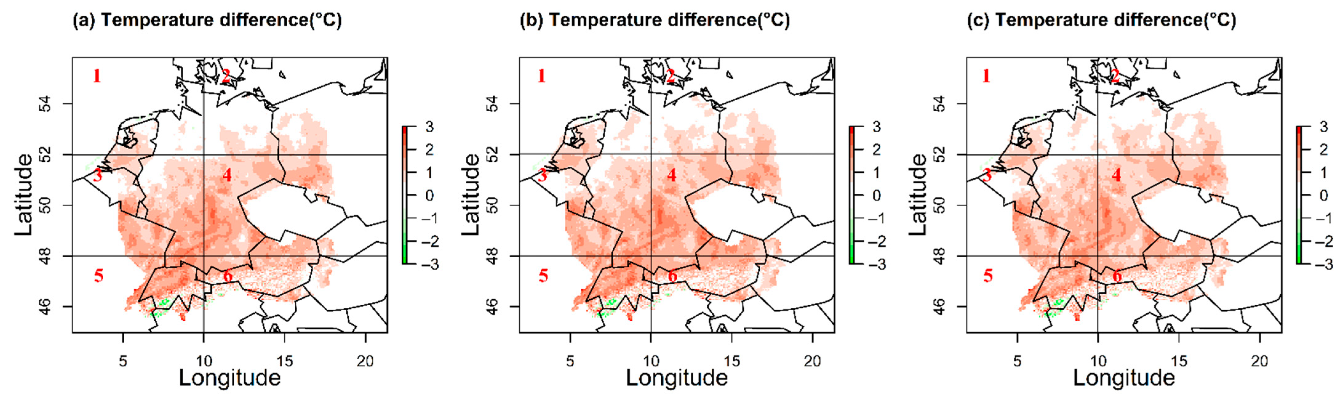
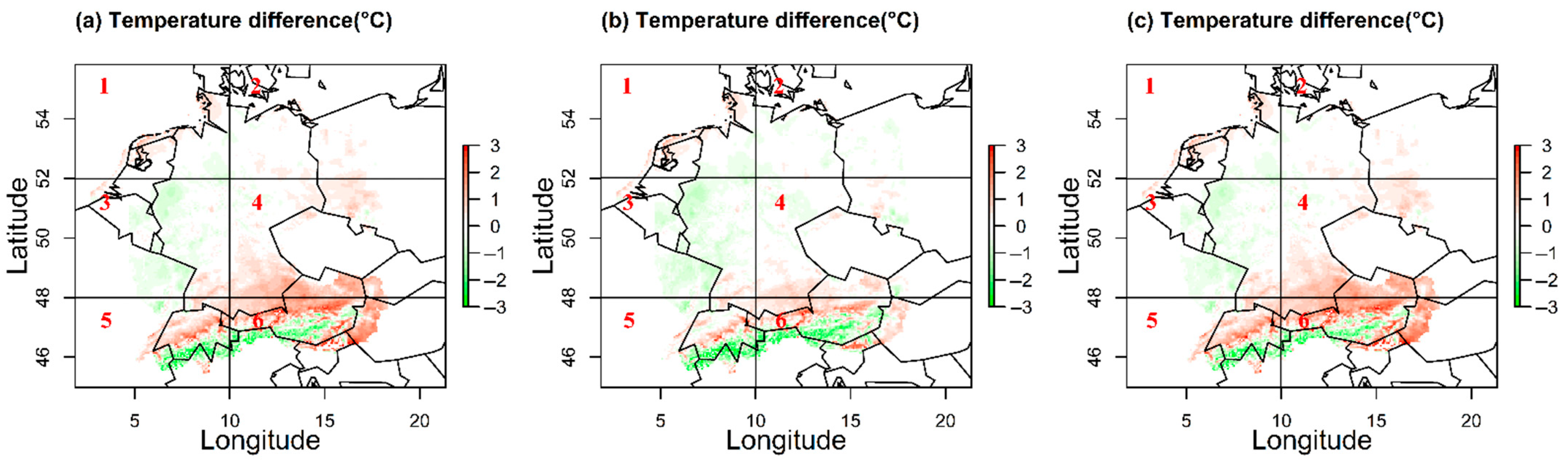
  • The temperature output from COSMO-CLM based on the three LC maps GlobCover 2009, GLC2000, and ESACCI-LC was compared with the observational data—HYRAS. We evaluated the COSMO-CLM results by comparing the mean temperature with the HYRAS observational data over Germany and the adjacent area: the Alpine area.
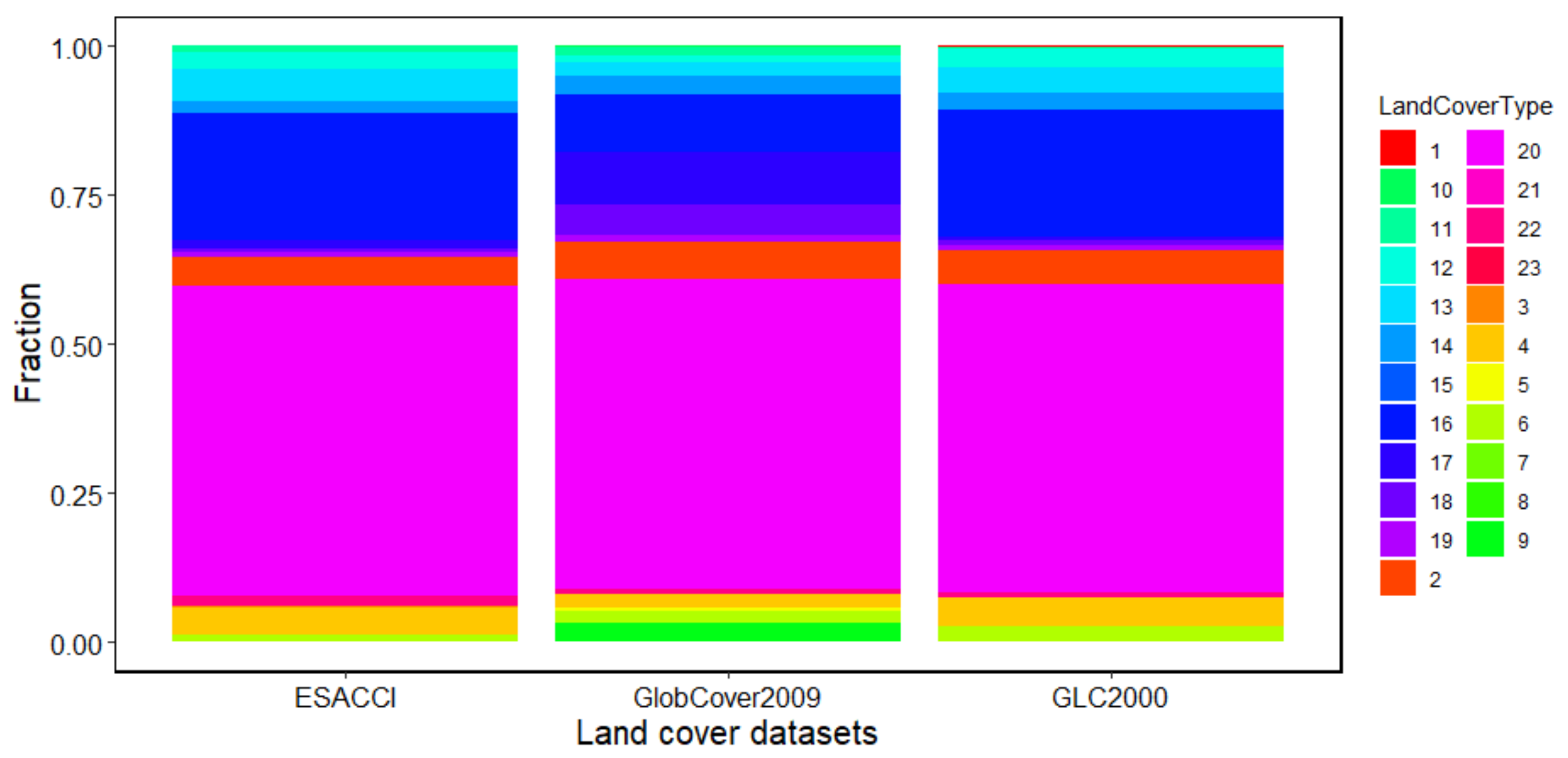
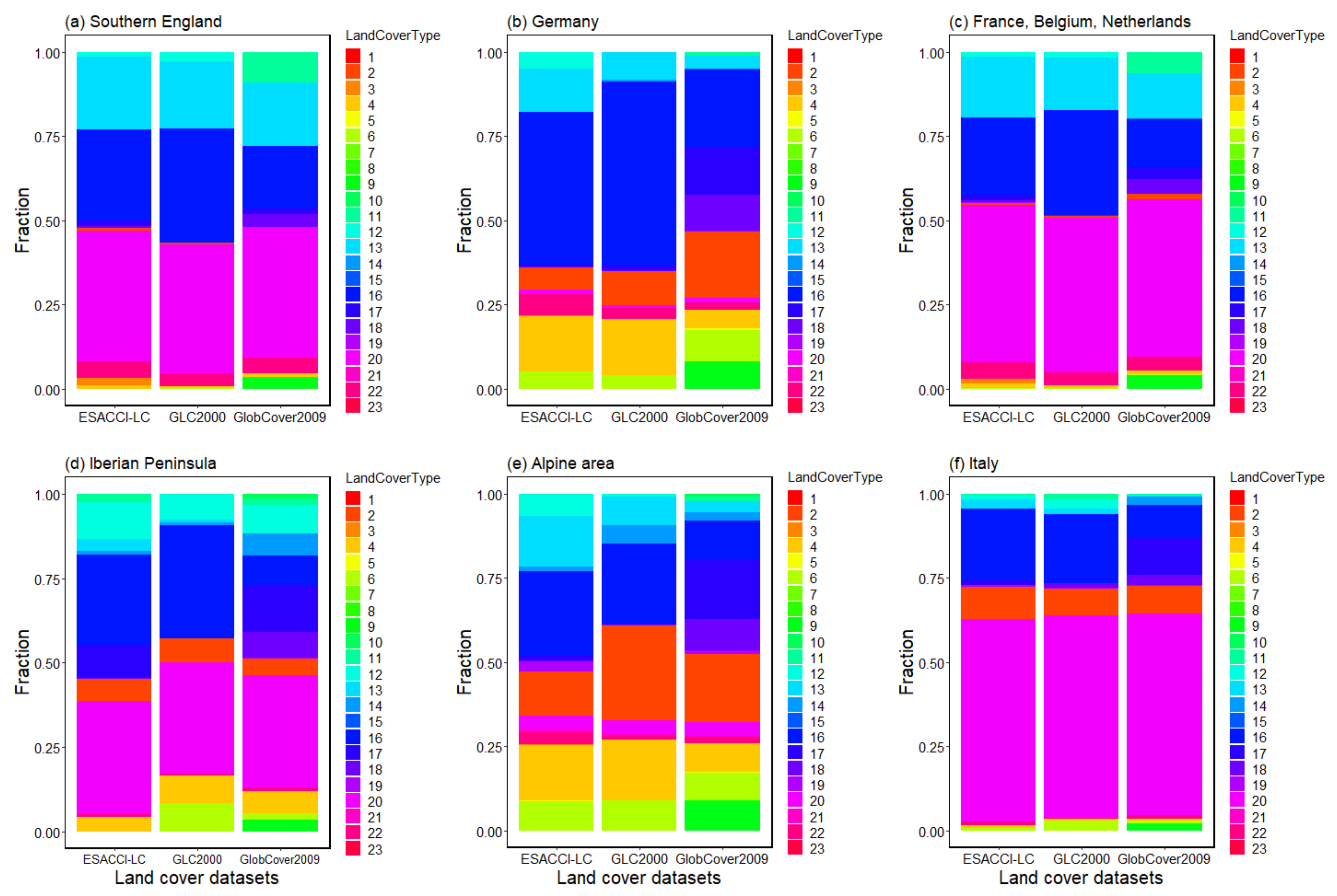
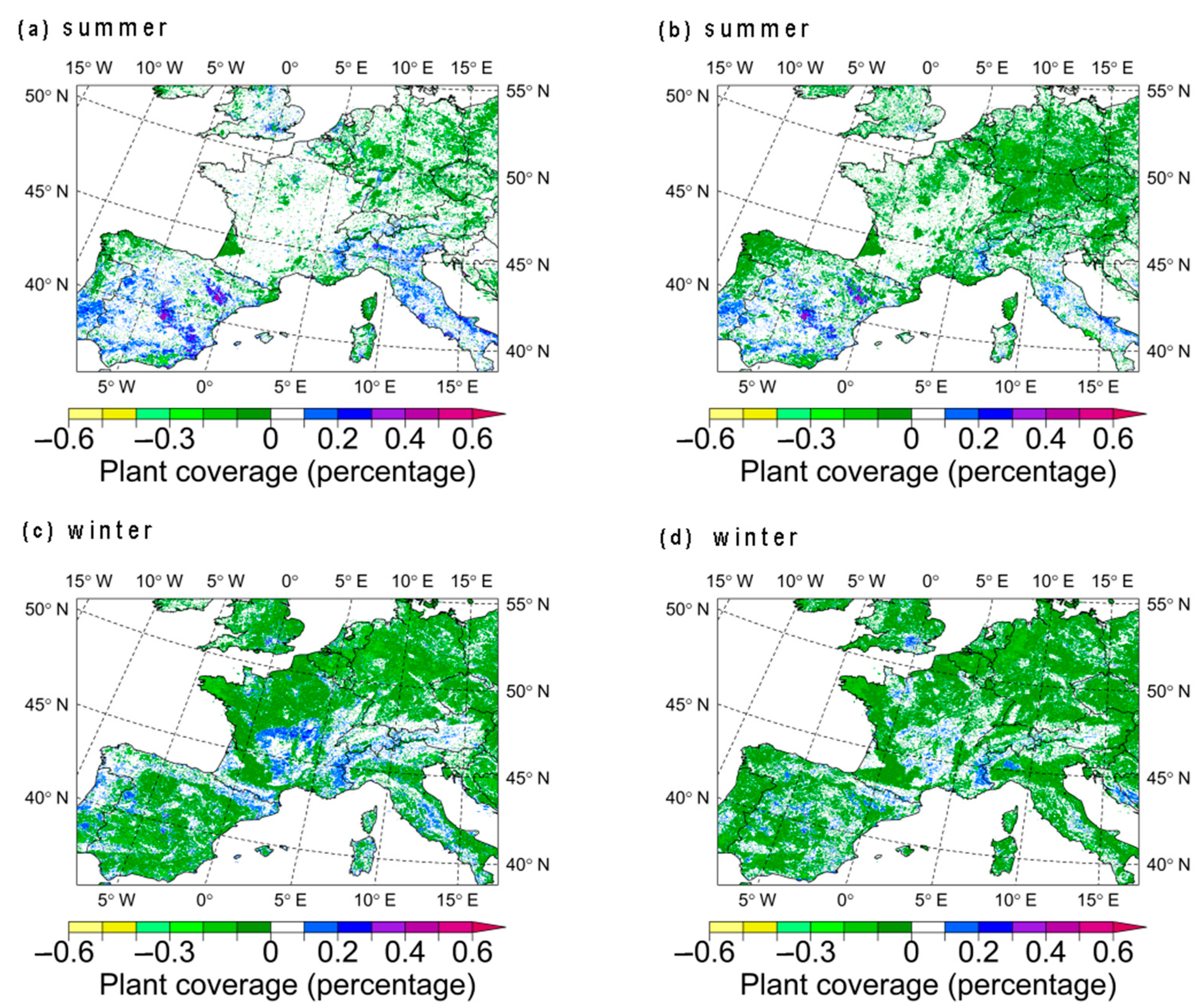
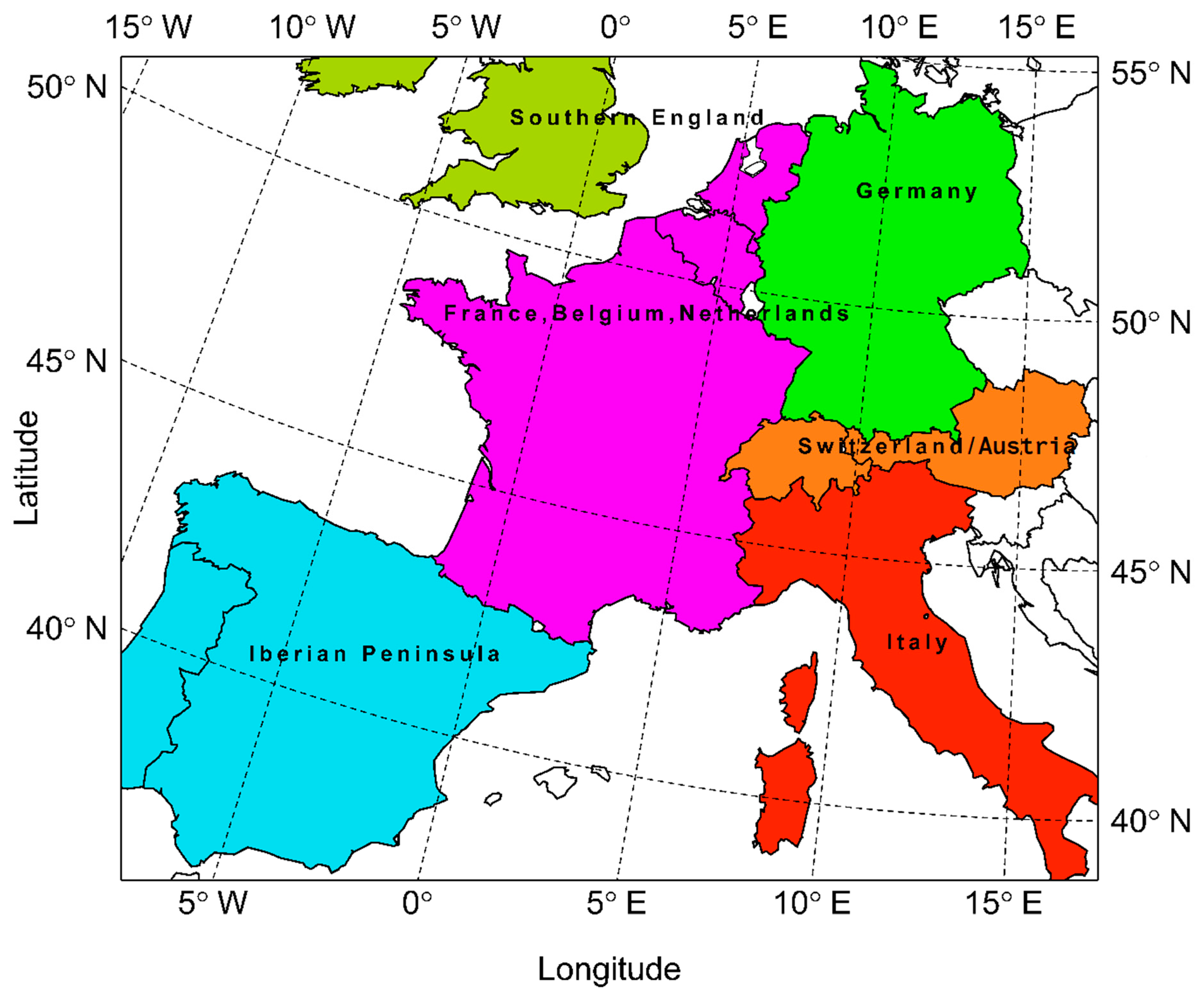
  • Comparison of the COSMO-CLM results between three land cover sets: In this part, we focused on the differences between the output plant coverage and LAI by setting GlobCover 2009 as the reference simulation. The research domain was divided into six sub-domains, and the LC fraction of each domain is shown in Figure 1.
  • The relation between the difference in the three LC data sets (LAI and plant coverage) and the simulated temperature are shown by scatter plots (Figure A1 and Figure A2).
We concentrated on summer (June, July, and August) 1999 and winter (December, January, and February) 1999/2000, investigating the impacts of different land cover maps and fractions on temperature, LAI, and plant cover. Furthermore, we also addressed the performance of COSMO-CLM in the two seasons.

3.4. Statistically Study

The performance of the three different land cover data sets was evaluated by the statistical significance t-test [54] and bias (calculated through mean bias error).
  • The differences of the three land cover data sets with respect to the reference simulation (HYRAS or GlobCover 2009) were statistically assessed with a one side t-test under the following null hypothesis: the target simulation is not different compared to the reference. The degrees of freedom for the t-test was calculated as n−2, where n is the grid number for each group.
  • For the evaluation of the simulated temperature, bias (see Equation (1)) was calculated through the sub-domain to see the average bias towards the observational data in the simulations. Where n indicates the total grid number, i indicates the specific grid box, and x presents the value of every grid box.
B i a s = 1 n i = 1 n x i x ¯

4. Results and Discussion

4.1. Evaluation of Simulated Temperature Based on the Three LC Maps

There were two main questions we sought to answer. Is the simulated temperature based on three different land cover maps reasonably simulated compared to the observational data? How does the temperature react to different land cover maps and fractions in the summer and winter seasons? To evaluate the simulations and study the temperature response to different LC maps and fractions, we first calculated the mean seasonal temperature difference between the three COSMO-CLM outputs and the observational data HYRAS for each grid point over the summer (JJA) in 1999 and winter (DJF) in 1999/2000 (Figure 3 and Figure 4).
In summer, the simulated mean temperature over southern Germany is overestimated by approximately 2 °C but underestimated in parts of the Alpine region (Figure 3). There are differences in the north of the sub-domain, where the difference in Figure 3a,c is not as high as in Figure 3b. This is interesting because GLC2000 and ESACCI-LC share similar land cover type fractions, as seen in Figure 1 and Figure 2b,e. These results demonstrate that apart from the LC fraction, it is also necessary to study the role of LC distribution in regional climate modeling.
Over the Alpine area, the simulated temperature shows differences ranging between −3 and +3 °C compared to the observed temperature (Figure 3). The orographic and soil moisture settings in the COSMO-CLM play an important role in affecting the temperature distribution. The long-term snow cover may also affect the temperature simulation in this case. Future studies should further investigate the relationship between the temperature and the elevation and soil moisture settings in COSMO-CLM.
The statistical significance test at the 95% confidence level for the simulated temperature difference to HYRAS and for each of the six sub-areas, as shown in Figure 3 and Figure 4, are presented in Table 4. Non-significant differences denote a good agreement between the simulations and the observations. In total, ESACCI-LC shows a better agreement with HYRAS compared to GlobCover 2009 and GLC2000. Over southwestern Germany (area 3, 3), ESACCI-LC indicates non-significant differences, while the GlobCover 2009 and GLC2000 simulated results show a noticeable difference to observations according to the significance t-test.
In winter (Figure 4), the simulated seasonal mean temperature is in good agreement with the observational data over most of the area, except for the Alpine area. The COSMO-CLM output temperature based on the ESACCI-LC is similar to GlobCover 2009 compared to GLC2000. Although the GLC2000 and ESACCI LC maps have a similar land cover fraction, the simulation output does not support this similarity, denoting that, the land cover fraction may not be the decisive component of the LC maps for the simulated temperature.
A much better performance is evident for all simulations with the different LC maps and all sub-regions during the winter season (Figure 3 and Table 5). The simulated temperature with ESACCI-LC shows more realistic results compared to HYRAS, except in areas 5 and 6. According to Table 5, the GlobCover 2009 and GLC2000 results show a remarkable difference over the whole region, especially over the south of Germany and the Alpine area. As for the summer analysis, a relationship between the LC fraction and the regional climate simulation in terms of seasonal temperature does not hold (Figure 3 and Table 4), which also reinforces the need to further investigate the effects of LC distributions.
We also calculated the overall bias for the six areas, as well as the whole domain (see Table 6). Table 6 indicates that the simulated temperature shows a greater difference in summer compared to winter. In summer, the temperature was overestimated by COSMO-CLM with three different land cover maps. In contrast, the winter temperature was mostly underestimated over Germany, except over the areas 5 and 6.
Overall, COSMO-CLM performs better in winter compared to summer. We expect this is because of the vegetation scheme, the parameterization of elevation change and the snow cover in COSMO-CLM. It is necessary to conduct further studies in this area.

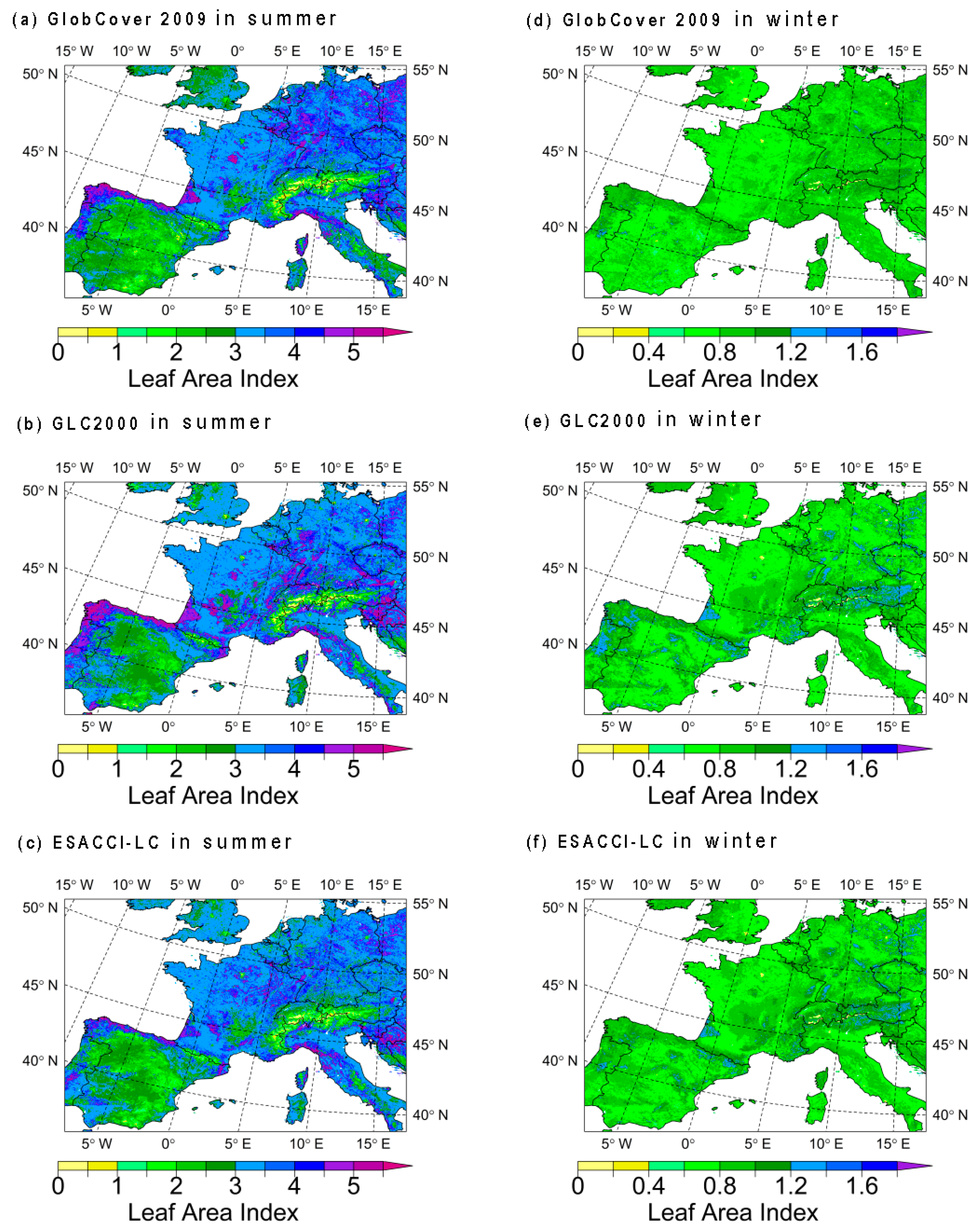
4.2. Impacts of Different Land Cover Types on the COSMO-CLM Output LAI

To answer the question on how the LAI (leaf area/ground area, m2/m2) react according to different land cover data sets, we compared the summer and winter LAI based on the three land cover data sets. The GlobCover 2009 data set has been used as the reference data.
The simulated summer and winter LAIs are shown in Figure 5. The simulations show an agreement over the European study area. Differences over specific areas, such as the Alps, northern Iberian Peninsula, smaller parts of Germany and France are more pronounced (±0.6 m2/m2) during the summer. During the winter, the LAI differences are significantly smaller (up to ±0.2 m2/m2) between the ESACCI-LC/GLC2000 and the GlobCover 2009.
The highest LAI differences are found in the summer over the Alpine area (Figure 5). These differences may be related to the orography, snow cover, and elevation parametrization in COSMO-CLM. The different classification systems that are used for the creation of the land cover maps may also impact the simulations as seen by the high differences over the northern Iberian Peninsula that is characterized by different land cover types due to the different classification systems used by the LC maps. In winter, the LAI distribution is more homogenous (Figure 5) indicating the higher sensitivity of the COSMO-CLM model during summer.
As for the temperature assessment, the European study has been divided into six different regions (see Figure A3 in Appendix A) according to the LC fraction differences in order to evaluate the COSMO-CLM output (LAI and plant cover) via a differences statistical significance test. The six areas: southern England, Germany, France with Belgium and the Netherlands, the Iberian Peninsula, Switzerland/Austria and the Alpine area, and Italy, are shown in Table 7 together with the t-test results for LAI. The areas of southern England, Germany, France with Belgium, and the Netherlands show good agreement between the two LC maps and the reference data set. Larger deviations are found over complex topography areas as the Iberian Peninsula, the Alpine area, and Italy. Over the complex orographically Alpine area, larger significant differences are found for both winter and summer.
In the summer, smaller differences characterize the ESACCI-LC simulations compared to GLC2000 over the areas with lower terrain complexity (Figure 6). The GLC2000 summer map shows a clear overestimation of the LAI over the Iberian Peninsula. The same map is characterized by a significant underestimation over the northern Alpine areas, in contrast to the overestimation of LAI over the southern rim. Most of the sub-regions show smaller LAI differences of around ±0.2 during winter with lower sensitivity to the two different land cover maps (Figure 6).

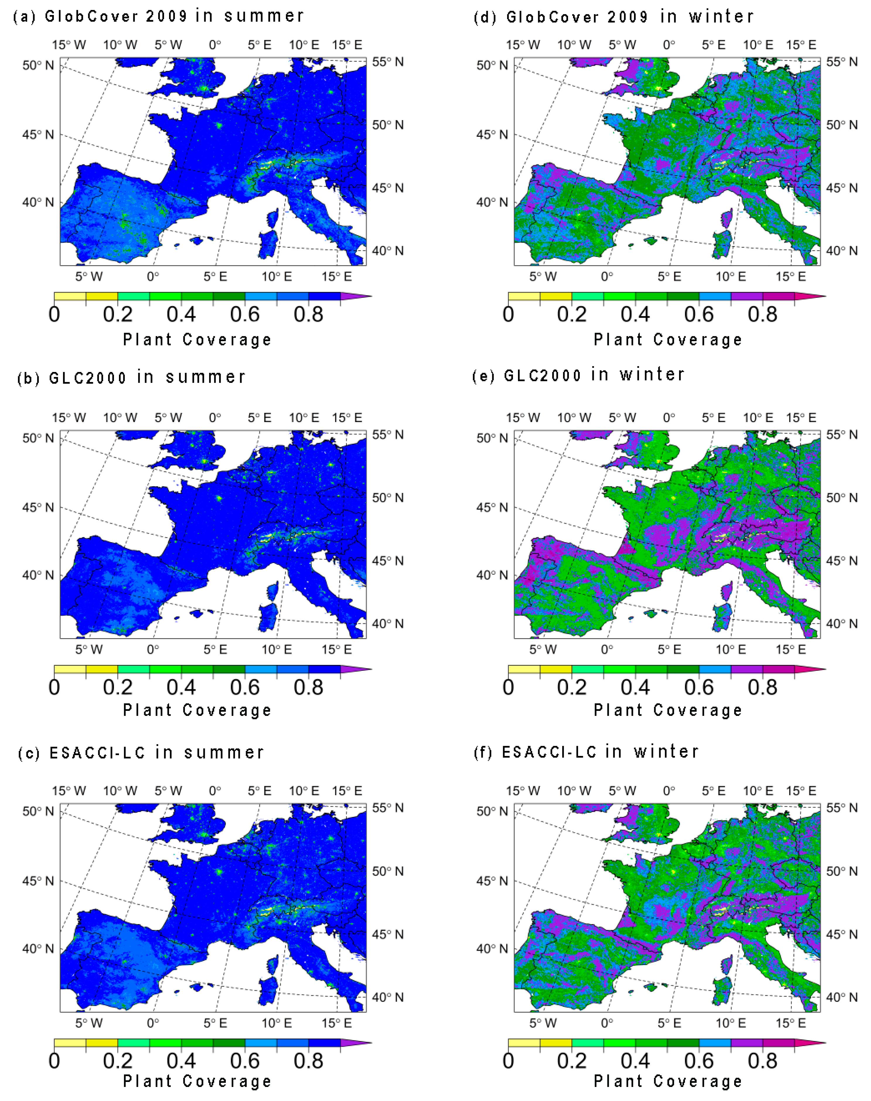
4.3. Impacts of Different Land Cover Types on the COSMO-CLM Output Plant Coverage

With the aim to investigate how the plant coverage is changing with the different land cover data sets, we compared the simulated summer and winter plant cover with three land cover data sets and looked at their differences with respect to the reference data set GlobCover 2009. Figure 7 presents the mean seasonal simulated plant coverage simulated with the three different land cover data sets (GlobCover 2009, GLC2000, and ESA-CCI-LC). It is obvious and expected that during winter, the plant coverage is lower than during the summertime, especially over central Europe (Germany, the Netherlands, and France). Seasonal vegetation, such as crops, which are under agricultural rest conditions during winter over these regions, is a major feature of this difference.
In the summer, the three simulations show similar plant coverage, while differences are concentrated over the Iberian Peninsula and the Alpine area (Figure 7). Lower plant coverage is produced over both areas with GlobCover 2009. In winter, the simulated plant coverage shows smaller differences between the three land cover data sets. Larger differences can be seen over the Alpine area (Figure 7), where the simulations show strong variation, mainly due to the high elevation range and the forest vegetation type. The Alpine area has different LC fractions because the land cover classification system varies among the LC maps (see Figure 2e). Further work should investigate the relationship between these.
The simulated plant coverage with ESACCI-LC is lower overall than the GlobCover 2009 both in summer and winter (Figure 8, Table 8). Plant coverage differences between the two simulations are maximized over the high plant coverage areas, compared to the lower plant coverage areas. Differences between GlobCover 2009 and GLC2000 are less pronounced. Nevertheless, the difference between the simulated plant coverage based on ESACCI-LC and GlobCover 2009 is not as obvious as it is between GLC2000 and GlobCover 2009. During summer, ESACCI-LC simulations seem to agree well with the reference map over most of the area, when compared with GLC2000 (Figure 8). The ESACCI-LC map performs better for plant coverage, especially in summer.

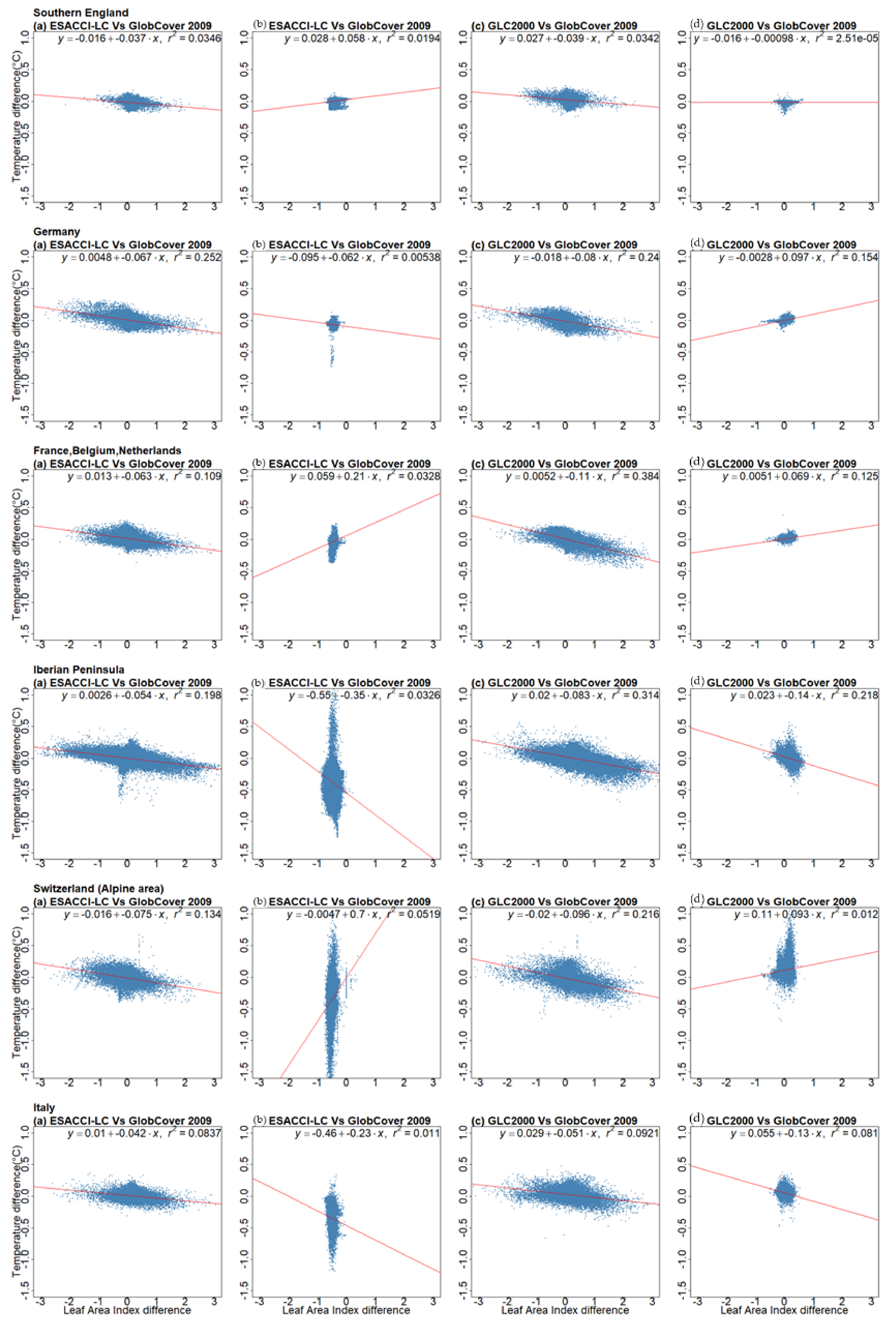
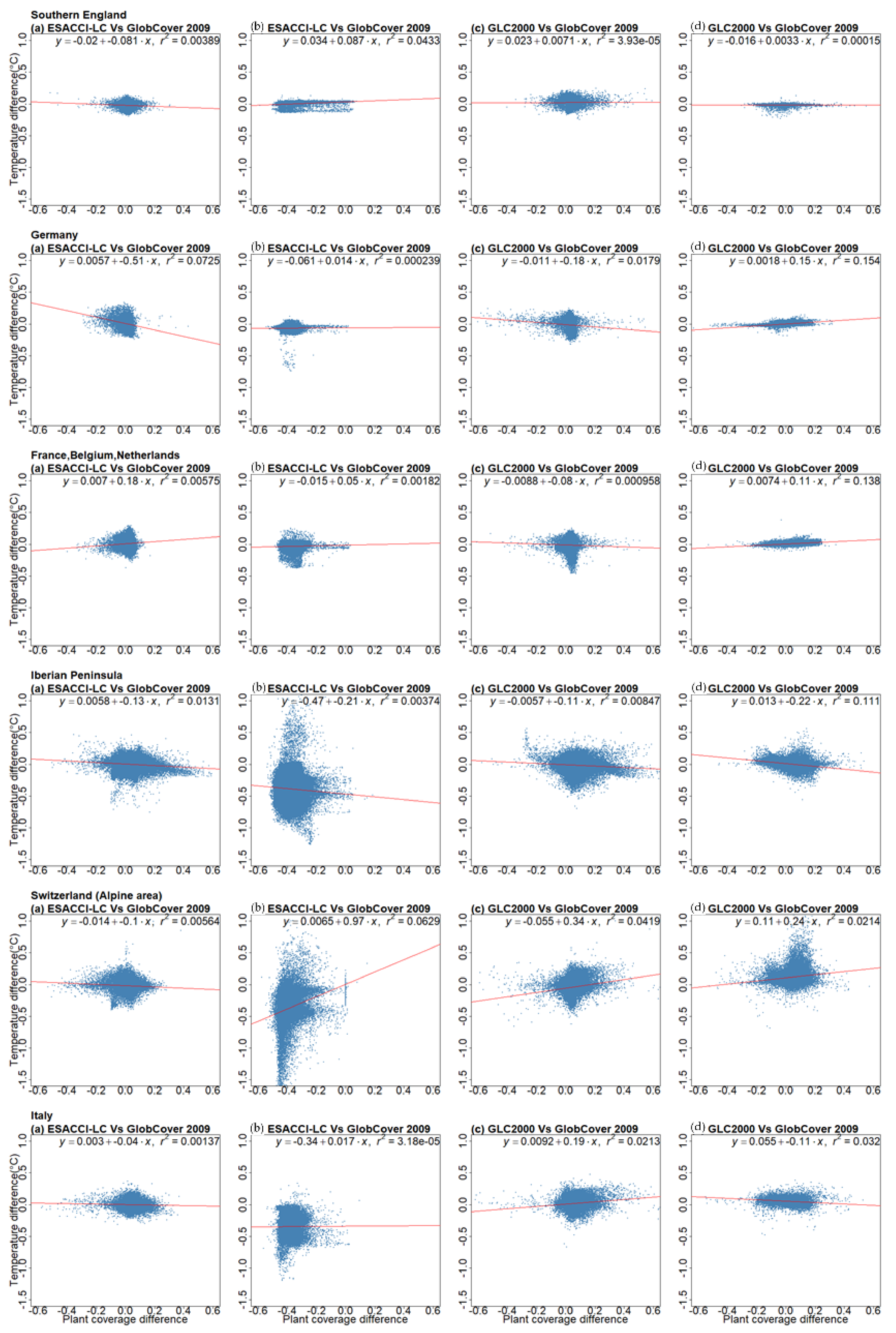
4.4. Relationship between Differences in Land Cover Data Sets and Differences in the Simulated Temperature

In this section, we address the connections between different land cover maps/fraction effects and temperature, LAI, and plant coverage in the COSMO-CLM regional climate simulation. LAI and plant coverage influence the evapotranspiration levels, where a higher LAI or plant coverage lead to higher evapotranspiration and greater evaporation reduces the air temperature, evaporation cooling, due to energy absorption. To investigate how the differences between the land cover data sets (LAI and plant coverage) translate into the differences seen in the simulated temperature, we prepared a scatter plot between the differences in land cover data and the simulated results in summer (Figure A1 in Appendix A) and winter (Figure A2 in Appendix A) of ESACCI-LC vs. GlobCover 2009 and GLC2000 vs. GlobCover 2009. We can see that the temperature is affected more by the LAI in summer (Figure A1a,c) and winter (Figure A2a,c). In summer, the temperature shows a negative relationship between the differences in the LAI and differences in temperature. This means that an increase in LAI results in a temperature decrease in the COSMO-CLM output. In winter, this relationship is not as distinct as in summer but still follows the same pattern [55]. The temperature does not react as much to plant coverage as to change in LAI during both seasons (Figure A1b,d and Figure A2b,d). A slightly negative relationship between plant coverage and temperature is seen in the winter.

4.5. Impact of the Classification System and Land Cover Unifying Methodology

As mentioned earlier, the land cover maps are produced with different classification systems. These classification systems are categorized into supervised (human-guided) and unsupervised (calculated by the software) [56,57]. Different classification systems result in differences in land cover maps both in terms of fraction and distribution by using even the same source data. The sensitivity of COSMO-CLM to different land cover maps and fractions is related also to the classification systems used to produce them. Therefore, to study the impacts of different LC maps on regional climate simulation, we unified the legend of the three used LC maps. By unifying the legend, we can compare the differences without concerning the non-identical land cover type definition of three land cover maps.
Further, re-gridding the three land cover maps into the same target horizontal resolution by EXTPAR because the different spatial resolutions could also influence the simulation results.

5. Conclusions

In this study, we applied three different LC maps (GlobCover 2009, GLC2000, and ESACCI-LC) as the lower boundary input data to perform simulations with COSMO-CLM over a large part of Europe at a 3 km horizontal resolution. The analysis of air temperature, LAI and plant coverage showed that COSMO-CLM is sensitive to different LC maps and fractions. A comparison of the simulated temperature output shows that all simulations with the three different LC maps provided reliable results compared to the observational data. The analysis also showed that the LAI and plant coverage have different feedback based on different land cover types, especially over the areas with high diversity in LC fractions (over southern Germany, and the Alpine area) and density vegetation coverage (e.g., over the northern Iberian Peninsula). Nevertheless, the simulated results indicate different feedback to different LC maps and fractions in summer and winter. Generally, the model performed better for the winter compared to the summer. The different regional representations of COSMO-CLM also indicate that the soil moisture, atmospheric circulation, evaporative demand, elevation, and snow cover schemes are located in the frame of land cover impacts. A comprehensive study of all of these factors is important in terms of high accuracy in climate modeling.
This study indicated that different LC maps and different LC fractions, as lower boundaries of COSMO-CLM have significant impacts on the simulated air temperature, the LAI, and plant coverage. The questions raised in the introduction can be answered as follows:
  • The seasonal temperature outputs of the COSMO-CLM based on these three data sets closely resemble the observations. Over most of the research domain, according to the temperature anomaly comparison with observational data, all three LC maps provided reliable COSMO-CLM simulation results. While over the Alpine area, the results showed higher deviation (differences of –3 to +3 K), further studies are needed to investigate the effects of soil moisture and orography on temperature.
  • The simulated temperature is sensitive to different land cover maps and fractions. The temperature shows higher dependence on land cover fractions in summer compared to winter.
  • Different LC maps affect the LAI, as well as the plant coverage. The regional and local simulation results responded differently towards the land cover maps and fractions. The area covered by forest with a heterogeneous land cover combination showed high sensitivities related to different land cover maps.
  • The COSMO-CLM output did not show a corresponding difference in the LC fraction. In our experiments, GLC2000 and ESACCI-LC showed similar LC fractions compared to GlobCover 2009, but the COSMO-CLM output showed greater similarity between ESACCI-LC and GlobCover 2009. This suggests that we not only need to check the differences in LC fraction but also the differences in LC distribution, and this will be the next step of our research.
In future studies, we will analyze how heterogeneous land cover types and seasonal land cover types affect climate and will also assess the role of land cover in regional climate modeling. Furthermore, how to select the appropriate land cover maps is in the scope of the study. Investigating how regional climate sensitively responds to different land cover distributions is necessary.

Author Contributions

Conceptualization: M.Z., M.H.T., and J.L.; methodology: M.Z., M.H.T. and J.L.; software development: M.Z., M.H.T., and E.H.; validation: M.Z.; analysis and statistical evaluation: M.Z., M.H.T., E.X., and J.L.; writing process and interpretation of results: all authors. All authors have read and agreed to the published version of the manuscript.

Funding

This research was funded by and the Justus Liebig University of Giessen and the German Research Foundation (DFG) grant number 401857120.

Institutional Review Board Statement

Not applicable.

Informed Consent Statement

Not applicable.

Data Availability Statement

Not applicable.

Acknowledgments

Computational resources were made available by the German Climate Computing Center (DKRZ) through support from the Federal Ministry of Education and Research in Germany (BMBF). We acknowledge the support of the German Weather Service, the ESA Climate Change Initiative—Land Cover led by UCLouvain (2017), ESA 2010, and UCLouvain, website: \href{http://due.esrin.esa.int/page_globcover.php}{ESA DUE GlobCover}, accessed on 17 December 2019, Global Land Cover 2000 database. European Commission, Joint Research Centre 2003 for supplying the research data and software which we have used in this paper. The SPOT/PROBA-V LAI data product was generated by the land service of Copernicus, the Earth Observation programme of the European Commission. The research leading to the current version of the LAI product has received funding from various European Commission Research and Technical Development programmes. The product is based on SPOT/VGT 1 km data ((c) CNES/PROBA-V 1 km data ((c) ESA and distributed by VITO) last access date: 28/9/2018. This research was funded by the German Research Foundation (DFG), grant number 401857120. The authors acknowledge Jürgen Helmert (German Met Office) for his important input to the different sections.

Conflicts of Interest

The authors declare no conflict of interest.

Abbreviations

LCLand Cover
GLC2000Global Land Cover Map for the year 2000
JRCJoint Research Center
COSMOConsortium for Small-scale Modeling
CCLMCOSMO model in Climate Mode
PFTsPlant Function Types
ESAEuropean Space Agency
CCIClimate Change Initiative
EOEarth Observation
UNFCCCUnited Nations Framework Convention on Climate Change
GCSGeographic Coordinate System
NWPNumerical Weather Prediction
EXTPARExternal Parameter for Numerical Weather Prediction and Climate Application
WCRPWorld Climate Research Programme
CORDEXCoordinated Regional Downscaling Experiment
CDDConsecutive Dry-Day
DKRZGerman Climate Computing Center
MBEMean Bias Error

Appendix A

Figure A1. (a) LAI differences between land cover ESACCI-LC and GlobCover 2009 vs. temperature differences of ESACCI-LC and GlobCover 2009 in summer. (b) LAI differences between land cover ESACCI-LC and GlobCover 2009 vs. temperature differences of ESACCI-LC and GlobCover 2009 in winter. (c) LAI differences between land cover GLC2000 and GlobCover 2009 vs. temperature differences of GLC2000 and GlobCover 2009 in summer. (d) LAI differences between land cover GlC2000 and GlobCover 2009 vs. temperature differences of GLC2000 and GlobCover 2009 in winter.
Atmosphere 12 01595 g0a1
Figure A2. (a) Plant coverage differences between land cover ESACCI-LC and GlobCover 2009 vs. temperature differences of ESACCI-LC and GlobCover 2009 in summer. (b) Plant coverage differences between land cover ESACCI-LC and GlobCover 2009 vs. temperature difference of ESACCI-LC and GlobCover 2009 in winter. (c) Plant coverage differences between land cover GLC2000 and GlobCover 2009 vs. temperature difference of GLC2000 and GlobCover 2009 in summer. (d) Plant coverage differences between land cover GLC2000 and GlobCover 2009 vs. temperature differences of GLC2000 and GlobCover 2009 in winter.
Atmosphere 12 01595 g0a2
Figure A3. Six sub-domains used in the LAI and plant cover analysis.
Atmosphere 12 01595 g0a3

Appendix B. Landcover Transfer Table

Value of LC (ESACCI-LC)Land Cover Type of ESACCI-LCValue of LC (GlobCover 2009)
GlobCover LC Type/ESACCI LC Type
Land Cover Type of GlobCover 2009Value of LC (GLC2000)Land Cover Type of GLC2000
10Cropland, rainfed14/2Rainfed croplands16cultivated and managed areas
11Herbaceous cover
12Tree or shrub cover
20Cropland, irrigated or post-flooding11/1irrigated croplands16cultivated and managed areas
30Mosaic cropland (>50%)/natural vegetation (tree, shrub, herbaceous cover) (<50%)20/3mosaic cropland (50–70%)—vegetation (20–50%)17mosaic crop/tree/natural vegetation
40Mosaic natural vegetation (tree, shrub, herbaceous cover) (>50%)/cropland (<50%)30/4mosaic vegetation (50–70%)—cropland (20–50%)18mosaic crop/shrub or grass
50Tree cover, broadleaved, evergreen, closed to open (>15%)40/5closed broadleaved evergreen forest1evergreen broadleaf tree
60Tree cover, broadleaved, deciduous, closed to open (>15%)50/6closed broadleaved deciduous forest2deciduous broadleaf tree closed
61Tree cover, broadleaved, deciduous, closed (>40%)
62Tree cover, broadleaved, deciduous, open (15–40%)60/7Open broadleaved deciduous forest3deciduous broadleaf tree open
70Tree cover, needleleaved, evergreen, closed to open (>15%)70/8Closed (>40%) needleleaved evergreen forest (>5 m)4evergreen needleleaf tree
71Tree cover, needleleaved, evergreen, closed (>40%)
72Tree cover, needleleaved, evergreen, open (15–40%)90/9
Open (15–40%) needleleaved deciduous or evergreen forest (>5 m)
5
deciduous needleleaf tree
80Tree cover, needleleaved, deciduous, closed to open (>15%)
81Tree cover, needleleaved, deciduous, closed (>40%)
82Tree cover, needleleaved, deciduous, open (15–40%)
90Tree cover, mixed leaf type (broadleaved and needleleaved)100/10mixed broadleaved and needleleaved forest6mixed leaf tree
100Mosaic tree and shrub (>50%) / herbaceous cover (<50%)110/11Mosaic Forest/Shrubland (50–70%)/Grassland (20–50%)11evergreen shrubs closed-open
110Mosaic herbaceous cover (>50%) / tree and shrub (<50%)120/12Mosaic Grassland (50–70%) / Forest/Shrubland (20–50%)9mosaic tree / other natural vegetation
120Shrubland130/13Closed to open (>15%) shrubland (<5 m)12deciduous shrubs closed-open
121Evergreen shrubland
122Deciduous shrubland
130Grassland140/14Closed to open (>15%) grassland13herbaceous cover closed-open
140Lichens and mosses150/15Sparse (>15%) vegetation (woody vegetation, shrubs, grassland)14sparse herbaceous or grass
150Sparse vegetation (tree, shrub, herbaceous cover) (<15%)
152Sparse shrub (<15%)
153Sparse herbaceous cover (<15%)
160Tree cover, flooded, fresh or brakish water160/16closed to open forest regulary flooded7fresh water flooded tree
170Tree cover, flooded, saline water170/17closed forest or shrubland permanently flooded8saline water flooded tree
180Shrub or herbaceous cover, flooded, fresh/saline/brackish water180/18Closed to open grassland regularly flooded15flooded shrub or herbaceous
190Urban areas190/19Artificial surfaces22artificial surfaces
200Bare areas150/15Sparse (>15%) vegetation (woody vegetation, shrubs, grassland)14sparse herbaceous or grass
201Consolidated bare areas
202Unconsolidated bare areas
210Water bodies210/21Water bodies20water bodies
220Permanent snow and ice220/22Permanent snow and ice21snow and ice
230undefined230/23undefined23undefined

References

  1. Wang, S.; Kang, S.; Zhang, L.; Li, F. Modelling Hydrological Response to Different Land-Use and Climate Change Scenarios in the Zamu River Basin of Northwest China. Hydrol. Process. Int. J. 2008, 22, 2502–2510. [Google Scholar] [CrossRef]
  2. Betts, R.A.; Falloon, P.D.; Goldewijk, K.K.; Ramankutty, N. Biogeophysical Effects of Land Use on Climate: Model Simulations of Radiative Forcing and Large-Scale Temperature Change. Agric. For. Meteorol. 2007, 142, 216–233. [Google Scholar] [CrossRef]
  3. Wramneby, A.; Smith, B.; Samuelsson, P. Hot Spots of Vegetation-Climate Feedbacks under Future Greenhouse Forcing in Europe. J. Geophys. Res. Atmos. 2010, 115, D21119. [Google Scholar] [CrossRef] [Green Version]
  4. Arora, V.K.; Montenegro, A. Small Temperature Benefits Provided by Realistic Afforestation Efforts. Nat. Geosci. 2011, 4, 514–518. [Google Scholar] [CrossRef]
  5. Davin, E.L.; Rechid, D.; Breil, M.; Cardoso, R.M.; Coppola, E.; Hoffmann, P.; Jach, L.L.; Katragkou, E.; de Noblet-Ducoudré, N.; Radtke, K.; et al. Biogeophysical Impacts of Forestation in Europe: First Results from the LUCAS (Land Use and Climate across Scales) Regional Climate Model Intercomparison. Earth Syst. Dyn. 2020, 11, 183–200. [Google Scholar] [CrossRef] [Green Version]
  6. Steiner, A.L.; Pal, J.S.; Rauscher, S.A.; Bell, J.L.; Diffenbaugh, N.S.; Boone, A.; Sloan, L.C.; Giorgi, F. Land Surface Coupling in Regional Climate Simulations of the West African Monsoon. Clim. Dyn. 2009, 33, 869–892. [Google Scholar] [CrossRef]
  7. Lu, L.; Pielke, R.A., Sr.; Liston, G.E.; Parton, W.J.; Ojima, D.; Hartman, M. Implementation of a Two-Way Interactive Atmospheric and Ecological Model and Its Application to the Central United States. J. Clim. 2001, 14, 900–919. [Google Scholar] [CrossRef]
  8. Davin, E.L.; Stöckli, R.; Jaeger, E.B.; Levis, S.; Seneviratne, S.I. COSMO-CLM2: A New Version of the COSMO-CLM Model Coupled to the Community Land Model. Clim. Dyn. 2011, 37, 1889–1907. [Google Scholar] [CrossRef] [Green Version]
  9. Pielke, R.A.; Avissar, R.; Raupach, M.; Dolman, A.J.; Zeng, X.; Denning, A.S. Interactions between the Atmosphere and Terrestrial Ecosystems: Influence on Weather and Climate. Glob. Chang. Biol. 1998, 4, 461–475. [Google Scholar] [CrossRef]
  10. Betts, R. Implications of Land Ecosystem-Atmosphere Interactions for Strategies for Climate Change Adaptation and Mitigation. Tellus B Chem. Phys. Meteorol. 2007, 59, 602–615. [Google Scholar] [CrossRef] [Green Version]
  11. Avissar, R.; Pielke, R.A. The Impact of Plant Stomatal Control on Mesoscale Atmospheric Circulations. Agric. For. Meteorol. 1991, 54, 353–372. [Google Scholar] [CrossRef]
  12. Bonan, G.B.; Levis, S.; Kergoat, L.; Oleson, K.W. Landscapes as Patches of Plant Functional Types: An Integrating Concept for Climate and Ecosystem Models. Glob. Biogeochem. Cycles 2002, 16, 5-1–5-23. [Google Scholar] [CrossRef] [Green Version]
  13. Feddema, J.J.; Oleson, K.W.; Bonan, G.B.; Mearns, L.O.; Buja, L.E.; Meehl, G.A.; Washington, W.M. The Importance of Land-Cover Change in Simulating Future Climates. Science 2005, 310, 1674–1678. [Google Scholar] [CrossRef] [Green Version]
  14. Luca, A.D.; Argüeso, D.; Evans, J.P.; de Elía, R.; Laprise, R. Quantifying the Overall Added Value of Dynamical Downscaling and the Contribution from Different Spatial Scales. J. Geophys. Res. Atmos. 2016, 121, 1575–1590. [Google Scholar] [CrossRef] [Green Version]
  15. Pitman, A.J. The Evolution of, and Revolution in, Land Surface Schemes Designed for Climate Models. Int. J. Climatol. J. R. Meteorol. Soc. 2003, 23, 479–510. [Google Scholar] [CrossRef]
  16. Brovkin, V.; Sitch, S.; Von Bloh, W.; Claussen, M.; Bauer, E.; Cramer, W. Role of Land Cover Changes for Atmospheric CO2 Increase and Climate Change during the Last 150 Years. Glob. Chang. Biol. 2004, 10, 1253–1266. [Google Scholar] [CrossRef] [Green Version]
  17. Seneviratne, S.I.; Corti, T.; Davin, E.L.; Hirschi, M.; Jaeger, E.B.; Lehner, I.; Orlowsky, B.; Teuling, A.J. Investigating Soil Moisture–Climate Interactions in a Changing Climate: A Review. Earth-Sci. Rev. 2010, 99, 125–161. [Google Scholar] [CrossRef]
  18. Stéfanon, M.; Schindler, S.; Drobinski, P.; de Noblet-Ducoudré, N.; Andrea, F.D. Simulating the Effect of Anthropogenic Vegetation Land Cover on Heatwave Temperatures over Central France. Clim. Res. 2014, 60, 133–146. [Google Scholar] [CrossRef]
  19. Giorgi, F.; Mearns, L.O. Approaches to the Simulation of Regional Climate Change: A Review. Rev. Geophys. 1991, 29, 191–216. [Google Scholar] [CrossRef]
  20. Tölle, M.H.; Gutjahr, O.; Busch, G.; Thiele, J.C. Increasing Bioenergy Production on Arable Land: Does the Regional and Local Climate Respond? Germany as a Case Study. J. Geophys. Res. Atmos. 2014, 119, 2711–2724. [Google Scholar] [CrossRef]
  21. Torma, C.; Giorgi, F.; Coppola, E. Added Value of Regional Climate Modeling over Areas Characterized by Complex Terrain—Precipitation over the Alps. J. Geophys. Res. Atmos. 2015, 120, 3957–3972. [Google Scholar] [CrossRef]
  22. Alestalo, M. The Energy Budget of the Earth–Atmosphere System in Europe. Tellus 1981, 33, 360–371. [Google Scholar] [CrossRef]
  23. Jacob, D.; Petersen, J.; Eggert, B.; Alias, A.; Christensen, O.; Bouwer, L.; Braun, A.; Colette, A.; Déqué, M.; Georgievski, G.; et al. EURO-CORDEX: New High-Resolution Climate Change Projections for European Impact Research. Reg. Environ. Chang. 2014, 14, 563–578. [Google Scholar] [CrossRef]
  24. Kotlarski, S.; Keuler, K.; Christensen, O.B.; Colette, A.; Déqué, M.; Gobiet, A.; Goergen, K.; Jacob, D.; Lüthi, D.; van Meijgaard, E.; et al. Regional Climate Modeling on European Scales: A Joint Standard Evaluation of the EURO-CORDEX RCM Ensemble. Geosci. Model Dev. 2014, 7, 1297–1333. [Google Scholar] [CrossRef] [Green Version]
  25. Diffenbaugh, N.S. Atmosphere-Land Cover Feedbacks Alter the Response of Surface Temperature to CO2 Forcing in the Western United States. Clim. Dyn. 2005, 24, 237–251. [Google Scholar] [CrossRef]
  26. Foley, J.A.; Levis, S.; Prentice, I.C.; Pollard, D.; Thompson, S.L. Coupling Dynamic Models of Climate and Vegetation. Glob. Chang. Biol. 1998, 4, 561–579. [Google Scholar] [CrossRef] [Green Version]
  27. Yokohata, T.; Kinoshita, T.; Sakurai, G.; Pokhrel, Y.; Ito, A.; Okada, M.; Masaki, T.I.; Nishimori, M.; Hanasaki, N.; Takahashi, K. MIROC-INTEG1: A Global Bio-Geochemical Land Surface Model with Human Water Management, Crop Growth, and Land-Use Change. Geosci. Model Dev. Discuss. 2019. [Google Scholar] [CrossRef] [Green Version]
  28. Tölle, M.H.; Engler, S.; Panitz, H.-J. Impact of Abrupt Land Cover Changes by Tropical Deforestation on Southeast Asian Climate and Agriculture. J. Clim. 2016, 30, 2587–2600. [Google Scholar] [CrossRef]
  29. Wilhelm, M.; Davin, E.L.; Seneviratne, S.I. Climate Engineering of Vegetated Land for Hot Extremes Mitigation: An Earth System Model Sensitivity Study. J. Geophys. Res. Atmos. 2015, 120, 2612–2623. [Google Scholar] [CrossRef]
  30. Fosser, G.; Khodayar, S.; Berg, P. Benefit of Convection Permitting Climate Model Simulations in the Representation of Convective Precipitation. Clim. Dyn. 2015, 44, 45–60. [Google Scholar] [CrossRef] [Green Version]
  31. Pal, S.; Chang, H.-I.; Castro, C.L.; Dominguez, F. Credibility of Convection-Permitting Modeling to Improve Seasonal Precipitation Forecasting in the Southwestern United States. Front. Earth Sci. 2019, 7, 11. [Google Scholar] [CrossRef] [Green Version]
  32. Meredith, E.P.; Ulbrich, U.; Rust, H.W.; Truhetz, H. Present and Future Diurnal Hourly Precipitation in 0.11° EURO-CORDEX Models and at Convection-Permitting Resolution. Environ. Res. Commun. 2021, 3, 055002. [Google Scholar] [CrossRef]
  33. Breil, M.; Rechid, D.; Davin, E.L.; de Noblet-Ducoudré, N.; Katragkou, E.; Cardoso, R.M.; Hoffmann, P.; Jach, L.L.; Soares, P.M.M.; Sofiadis, G.; et al. The Opposing Effects of Reforestation and Afforestation on the Diurnal Temperature Cycle at the Surface and in the Lowest Atmospheric Model Level in the European Summer. J. Clim. 2020, 33, 9159–9179. [Google Scholar] [CrossRef]
  34. Heck, P.; Lüthi, D.; Wernli, H.; Schär, C. Climate Impacts of European-Scale Anthropogenic Vegetation Changes: A Sensitivity Study Using a Regional Climate Model. J. Geophys. Res. Atmos. 2001, 106, 7817–7835. [Google Scholar] [CrossRef]
  35. Garnaud, C.; Sushama, L.; Verseghy, D. Impact of Interactive Vegetation Phenology on the Canadian RCM Simulated Climate over North America. Clim. Dyn. 2015, 45, 1471–1492. [Google Scholar] [CrossRef] [Green Version]
  36. Wouters, H.; Varentsov, M.; Blahak, U.; Schulz, J.-P.; Schattler, U.; Bucchignani, E.; Demuzere, M. User Guide for TERRA URB v2.2: The Urban-Canopy Land-Surface Scheme of the COSMO Model. 12p. Available online: http://cosmo-model.cscs.ch/content/tasks/workGroups/wg3b/docs/terra_urb_user.pdf (accessed on 24 November 2021).
  37. GLOBCOVER Products Description and Validation Report. Available online: https://www.researchgate.net/profile/O_Arino/publication/260137807_GLOBCOVER_products_description_and_validation_report/links/576bf8a808aef0e50da8a271/GLOBCOVER-products-description-and-validation-report.pdf (accessed on 25 May 2020).
  38. Arino, O.; Perez, J.R.; Kalogirou, V.; Defourny, P.; Achard, F. GlobCover 2009. Available online: https://epic.awi.de/id/eprint/31046/1/Arino_et_al_GlobCover2009-a.pdf (accessed on 25 May 2020).
  39. Yin, K.; Xu, S.; Zhao, Q.; Huang, W.; Yang, K.; Guo, M. Effects of Land Cover Change on Atmospheric and Storm Surge Modeling during Typhoon Event. Ocean Eng. 2020, 199, 106971. [Google Scholar] [CrossRef]
  40. Zhong, Y.; Luo, C.; Hu, X.; Wei, L.; Wang, X.; Jin, S. Cropland Product Fusion Method Based on the Overall Consistency Difference: A Case Study of China. Remote Sens. 2019, 11, 1065. [Google Scholar] [CrossRef] [Green Version]
  41. Bartholomé, E.; Belward, A.S. GLC2000: A New Approach to Global Land Cover Mapping from Earth Observation Data. Int. J. Remote Sens. 2005, 26, 1959–1977. [Google Scholar] [CrossRef]
  42. Lamarche, C.; Santoro, M.; Bontemps, S.; D’Andrimont, R.; Radoux, J.; Giustarini, L.; Brockmann, C.; Wevers, J.; Defourny, P.; Arino, O. Compilation and Validation of SAR and Optical Data Products for a Complete and Global Map of Inland/Ocean Water Tailored to the Climate Modeling Community. Remote Sens. 2017, 9, 36. [Google Scholar] [CrossRef] [Green Version]
  43. Bounoua, L.; DeFries, R.; Collatz, G.J.; Sellers, P.; Khan, H. Effects of Land Cover Conversion on Surface Climate. Clim. Chang. 2002, 52, 29–64. [Google Scholar] [CrossRef]
  44. Rauthe, M.; Steiner, H.; Riediger, U.; Mazurkiewicz, A.; Gratzki, A. A Central European Precipitation Climatology—Part I: Generation and validation of a high-resolution gridded daily data set (HYRAS). Meteorol. Z. 2013, 22, 235–256. [Google Scholar] [CrossRef]
  45. Tiedtke, M. Parameterization of Cumulus Convection in Large-Scale Models. In Physically-Based Modelling and Simulation of Climate and Climatic Change: Part 1; Schlesinger, M.E., Ed.; NATO ASI Series; Springer: Dordrecht, The Netherlands, 1988; pp. 375–431. ISBN 978-94-009-3041-4. [Google Scholar]
  46. Rockel, B.; Will, A.; Hense, A. Regional Climate Modelling with COSMO-CLM (CCLM). Meteorol. Z. 2008, 17, 347–348. [Google Scholar] [CrossRef]
  47. Schulz, J.-P.; Vogel, G.; Becker, C.; Kothe, S.; Rummel, U.; Ahrens, B. Evaluation of the Ground Heat Flux Simulated by a Multi-Layer Land Surface Scheme Using High-Quality Observations at Grass Land and Bare Soil. Meteorol. Z. 2016, 25, 607–620. [Google Scholar] [CrossRef]
  48. Ritter, B.; Geleyn, J.-F. A Comprehensive Radiation Scheme for Numerical Weather Prediction Models with Potential Applications in Climate Simulations. Mon. Weather Rev. 1992, 120, 303–325. [Google Scholar] [CrossRef] [Green Version]
  49. Young, K.C. A Numerical Simulation of Wintertime, Orographic Precipitation: Part I. Description of Model Microphysics and Numerical Techniques. J. Atmos. Sci. 1974, 31, 1735–1748. [Google Scholar] [CrossRef] [Green Version]
  50. Smiatek, G.; Rockel, B.; Schättler, U. Time Invariant Data Preprocessor for the Climate Version of the COSMO Model (COSMO-CLM). Meteorol. Z. 2008, 17, 395–405. [Google Scholar] [CrossRef]
  51. Smiatek, G.; Helmert, J.; Gerstner, E.-M. Impact of Land Use and Soil Data Specifications on COSMO-CLM Simulations in the CORDEX-MED Area. Meteorol. Z. 2016, 25, 215–230. [Google Scholar] [CrossRef]
  52. Asensio, H.; Messmer, M. External Parameters for Numerical Weather Prediction and Climate Application EXTPAR v5_0: User and Implementation Guide. 45p. Available online: http://www.cosmo-model.org/content/support/software/ethz/EXTPAR_user_and_implementation_manual_202003.pdf (accessed on 24 November 2021).
  53. Dee, D.P.; Uppala, S.M.; Simmons, A.J.; Berrisford, P.; Poli, P.; Kobayashi, S.; Andrae, U.; Balmaseda, M.A.; Balsamo, G.; Bauer, D.P. The ERA-Interim Reanalysis: Configuration and Performance of the Data Assimilation System. Q. J. R. Meteorol. Soc. 2011, 137, 553–597. [Google Scholar] [CrossRef]
  54. Welch, B.L. The Generalization of ‘Student’s’ Problem When Several Different Population Variances Are Involved. Biometrika 1947, 34, 28–35. [Google Scholar] [CrossRef]
  55. Hartmann, E.; Schulz, J.-P.; Seibert, R.; Schmidt, M.; Zhang, M.; Luterbacher, J.; Tölle, M.H. Impact of Environmental Conditions on Grass Phenology in the Regional Climate Model COSMO-CLM. Atmosphere 2020, 11, 1364. [Google Scholar] [CrossRef]
  56. Jog, S.; Dixit, M. Supervised Classification of Satellite Images. In Proceedings of the 2016 Conference on Advances in Signal Processing (CASP), Pune, India, 9–11 June 2016; pp. 93–98. [Google Scholar]
  57. Bernabé, S.; Plaza, A. A New System to Perform Unsupervised and Supervised Classification of Satellite Images from Google Maps. In Satellite Data Compression, Communications, and Processing VI; SPIE: Bellingham, WA, USA, 2010; Volume 7810, pp. 261–270. [Google Scholar]
Figure 1. Land cover data sets of the fraction of three land cover maps over the whole study area based on unified land cover types (see Appendix B).
Atmosphere 12 01595 g001
Figure 2. Land cover data sets of the fraction of three land cover maps over six different study areas based on unified land cover types (see Appendix B); (a) Southern England; (b) Germany; (c) France, Belgium, and Netherlands; (d) Iberian Peninsula; (e) Switzerland/Austria (the Alpine area); and (f) Italy.
Atmosphere 12 01595 g002
Figure 3. Summer 1999 mean temperature differences between simulations and HYRAS observations: (a) GlobCover2009, (b) GLC2000, and (c) ESACCI-LC. Numbers 1 to 6 refer to the six different sub-regions used to conduct the statistical significance test (Table 4).
Atmosphere 12 01595 g003
Figure 4. Winter 1999/2000 mean temperature differences between simulations and HYRAS observations: (a) GlobCover2009, (b) GLC2000, and (c) ESACCI-LC. Numbers 1 to 6 refer to six different sub-regions used to conduct the statistical significance test (Table 5).
Atmosphere 12 01595 g004
Figure 5. Simulated winter and summer LAI: (a) summer GlobCover2009, (b) summer ESACCI-LC, (c) summer GLC2000, (d) winter GlobCover2009, (e) winter ESACCI-LC, and (f) winter GLC2000.
Atmosphere 12 01595 g005
Figure 6. Winter and summer simulated LAI deviations with respect to GlobCover 2009: (a) ESACCI-LC summer, (b) GLC2000 summer, (c) ESACCI-LC winter and (d) GLC2000 winter.
Atmosphere 12 01595 g006
Figure 7. Seasonal simulated plant coverage: (a) GlobCover2009 in summer, (b) ESACCI-LC in summer, (c) GLC2000 in summer, (d) GlobCover2009 in winter, (e) ESACCI-LC in winter, and (f) GLC2000 in winter.
Atmosphere 12 01595 g007
Figure 8. Winter and summer simulated plant coverage deviations with respect to GlobCover 2009: (a) ESACCI-LC summer, (b) GLC2000 summer, (c) ESACCI-LC winter, and (d) GLC2000 winter.
Atmosphere 12 01595 g008
Table 1. Characteristics of the three different land cover data sets used in this study: GlobCover 2009 [42], GLC2000 [43], and ESACCI-LC [36], created by author.
Characteristics/Data SetESACCI-LCGLC2000GlobCover2009
Data SourceSatellite, observationSPOT4MERIS
Time Span1992–201520002009
Temporal ResolutionYearly----
Land Use/Cover Types372323
Spatial Resolution300 m1 km300 m
Classification SystemUnsupervisedUnsupervisedUnsupervised and supervised
Data FormatTiff/netCDFESRI/BinaryTiff
Table 2. Input parameters for start EXTPAR software.
ParametersInput Data
Topography dataGLOBE
Soil mapFAO digital soil map of the world
NDVI (normalized differential vegetation index)NDVI Climatology from NASA
Lake fractionGlobal lake database (DWD, RSHU, MétéoFrance)
AlbedoMODIS albedo (NASA)
Table 3. COSMO-CLM simulation set up.
ParametersInput Setting
InterpolationINT2LM-v2.05 clm15
ForcingERA-Interim
External dataGlobCover2009, GLC2000, ESACCI-LC
DomainMiddle Europe, approximately 3 km (0.0275°), 740 × 600 grid points
Time integrationTwo time-level Runge–Kutta schemes
Model time step25 s
ConvectionShallow convection based on Tiedtke scheme
Simulation period1999.01.01 to 2000.03.31
Table 4. Statistical significance test results (t-value) of the summer temperature differences (°C) between the simulated temperature and the HYRAS observations: Critical t-value = 1.960; results lower than the t-value are marked with * and are in bold.
GlobCover 2009GLC2000ESACCI-LC
Area 136.635.536.5
Area 222.42526.9
Area 338.436.4–18.4 *
Area 466.975.239.1
Area 526.025.5–75.6 *
Area 657.259.527.7
Table 5. Statistical significance test results (t-value) of the winter temperature differences (°C) between the simulated temperature and the HYRAS observations: Critical t-value = 1.960; results lower than the t-value are marked with * and are in bold.
GlobCover 2009GLC2000ESACCI-LC
Area 1–8.8 *–7.6 *–12.6 *
Area 215.915.613.5
Area 39.712.3–4.42 *
Area 411.69.8–0.6 *
Area 530.031.4–0.4 *
Area 623.623.85.1
Table 6. The bias of the simulated temperature compared to HYRAS over the six areas, as well as the whole area, both in summer and in winter.
SummerWinter
ESACCI-LCGlC2000GlobCover 2009ESACCI-LCGlC2000GlobCover 2009
Area 11.251.181.24–0.33–0.14–0.17
Area 20.590.540.49–0.12–0.07–0.06
Area 31.261.151.23–0.030.370.32
Area 40.650.650.57–0.100.0030.02
Area 50.970.850.880.181.101.05
Area 60.940.910.88–0.060.240.23
Whole region0.950.890.89–0.090.170.16
Table 7. Statistical significance test results (t-value) of the LAI differences between two land cover data sets and GlobCover 2009. Results lower than the critical t-value (1.960) are marked with * and are in bold.
SummerWinter
t-valueESACCI-LCGLC2000ESACCI-LCGLC2000
Southern England26.–62.5 *–38.0 *–39.1 *
Germany3.1–17.5 *–15.0 *8.6
France, Belgium, and the Netherlands−9.0 *1.5–51.5 *4.7
Iberian Peninsula10.829.915.113.9
Switzerland/Austria 57.922.48.540.3
Italy35.610.7–9.3 *56.6
Table 8. Statistical significance test results (t-value) of the plant cover differences between two land cover data sets and GlobCover 2009. Results lower than the critical t-value (1.960) are marked with * and are in bold.
SummerWinter
t-valueESACCI-LCGLC2000ESACCI-LCGLC2000
Southern England–27.7 *–23.2 *4.5–64.2 *
Germany–3.9 *10.216.1–0.6 *
France, Belgium, and the Netherlands–9.7 *22.6–9.9 *–40.839 *
Iberian Peninsula–1.5 *–0.2 *10.7–14.9 *
Switzerland/Austria 13.641.638.9–8.2 *
Italy17.438.825.62.3
Publisher’s Note: MDPI stays neutral with regard to jurisdictional claims in published maps and institutional affiliations.

