
Error Correction of Water Vapor Radiometers for VLBI Observations in Deep-Space Networks

1
Department of Electronics and Communication, Nanjing University of Information Science and Technology, Nanjing 210044, China
2
China Research Institute of Radiowave Propagation, Qingdao 266107, China
3
National Astronomical Observatories, Chinese Academy of Sciences, Beijing 100012, China
*
Authors to whom correspondence should be addressed.
Atmosphere 2021, 12(12), 1601; https://0-doi-org.brum.beds.ac.uk/10.3390/atmos12121601
Submission received: 2 November 2021
/
Revised: 27 November 2021
/
Accepted: 28 November 2021
/
Published: 30 November 2021
(This article belongs to the Special Issue Radiation and Radiative Transfer in the Earth Atmosphere)
Abstract
:In this paper, we present the design and implementation tests of a water vapor radiometer (WVR) suitable for very long baseline interferometry (VLBI) observation. We describe the calibration method with an analysis of the sources of measurement errors. The experimental results show that the long-term measurement accuracy of the brightness temperature of the water vapor radiometer can reach 0.2 K under arbitrary ambient conditions by absolute calibration, receiver gain error calibration, and antenna feeder system temperature noise error calibration. Furthermore, we present a method for measurements of the calibration error of the oblique path measurement. This results in an oblique path wet delay measurement accuracy of the water vapor radiometer reaching 20 mm (within one month).
1. Introduction
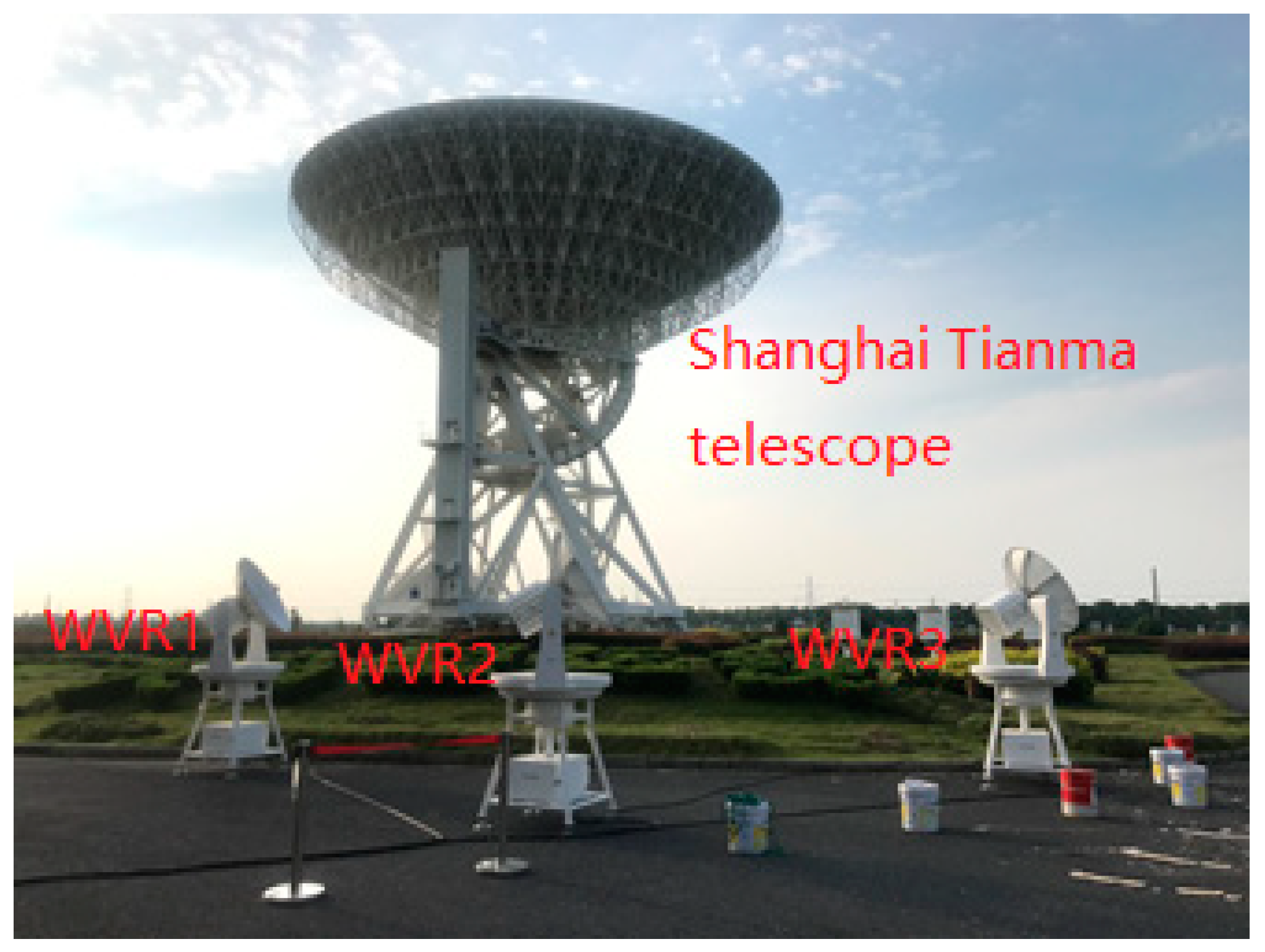
Studies of spacecraft tracking techniques have shown that the delay in the radiometric signal caused by changes in the refractive index of the troposphere is a major source of error in very long baseline interferometry (VLBI). VLBI astronomical measurements have shown that the observed coherence time is limited and that the delay rate is mainly caused by phase fluctuations in the Earth’s troposphere [1,2,3,4,5]. The microwave frequency signal used in the measurements and control will cause a refraction delay of approximately 6–7 ns along the zenith direction when penetrating the troposphere, which corresponds to a path length of approximately 2.3 m. At microwave frequencies, any accurate phase or delay measurements involving signals propagating between space and the ground must include methods to calibrate tropospheric effects. Tropospheric delays can be divided into dry and wet delays. Under the assumption of a hydrostatic equilibrium, the dry delay can be derived from the model by means of known surface pressures. In China, the error of the dry delay produced by using the Saastamoinen model is less than 1 mm. Due to the frequent changes in water vapor in the atmosphere and the inhomogeneous distribution height, almost all of the high-frequency spatial and temporal variations of the total tropospheric path delay are caused by the variations of the wet delay. The deep-space VLBI mission requires precise measurements of the radio signal path delay caused by water vapor in the atmosphere. The main instruments for the measurements are the water vapor radiometer (WVR) and the global navigation satellite system (GNSS). Among them, the water vapor radiometer can measure the wet delay in the troposphere in real time and can reduce the wet delay error to less than 1 cm [2]. The Jet Propulsion Laboratory (JPL) developed the earliest WVR and operated it from 1993 at Deep-Space Station 13 with a measurement delay error of approximately 20 mm. Keihm et al. used the WVR to analyze atmospheric tropospheric delays throughout 1994 [3]. In mid-1990, JPL developed the advanced water vapor radiometer (AWVR) with a stable narrow beam gain that can accurately estimate the propagation delay of water vapor in a semi-dry atmosphere with an accuracy of 1 mm [1]. Linfield et al. performed a water-vapor-radiometer-based tropospheric calibration experiment using VLBI observations over a 21 km baseline. They discussed sources of error, such as gain error, pointing error, and absorption model error, in wet path delay measurements of the AWVR [2]. David et al. investigated the dual water vapor radiometer (DWVR) deployed at the Venus Goldstone site in 2008. The data processing method is given and the effect of error sources, such as injected liquid water, has been studied [4]. The team at Chinese Academy of Sciences (CAS) built the VLBI network, which is mainly used for astronomy. By combining the CAS VLBI network with the TT&C network, the orbit determination missions of Chang’e 1 to 4 were successfully accomplished. Since Chang’e-3, the water vapor radiometer has been added to improve the accuracy of the VLBI measurement delay. Figure 1 shows three water vapor radiometers equipped with the Shanghai Tianma telescope. The QFW-6000 series and HZD-X series microwave radiometers used for meteorological observation and deep-space VLBI observation were developed by China Research Institute of Radiowave Propagation (CRIRP). The HZD-X water vapor radiometer introduced in this paper is a prototype water vapor radiometer developed specifically for the deep-space VLBI observation network in China. It can correct the wet delay in the zenith direction to less than 15 mm and the dry region can be reduced to less than 10 mm. In Section 2, the basic principle and design scheme of the water vapor radiometer are presented. In Section 3, the analyses of the sources of measurement errors are described and the correction methods for the errors are given. These analyses are based on experimental results and can be effectively applied to engineering, instead of simply discussing error sources that cannot be applied in practice.
2. WVR Design
Microwave radiometers are different from conventional radar or communication receivers. The signal received by a microwave radiometer is usually much lower than the noise power of the receiver. The antenna of a microwave radiometer receives incoherent thermal radiation signals from the target or scene under test and the transmitting medium, which are processed by the radiometer receiver and usually converted to an output voltage. In theory, as long as the receiver is in the use of a square law detector and linear amplifier, the receiver output voltage is linear with the antenna-received power or antenna temperature. When the microwave radiometer aims at the target or scene, we can calculate the antenna temperature based on the calibration equation and the output voltage of the radiometer and can retrieve the radiation brightness temperature or other parameters of the target or scene. This is the basic principle of the microwave radiometer.
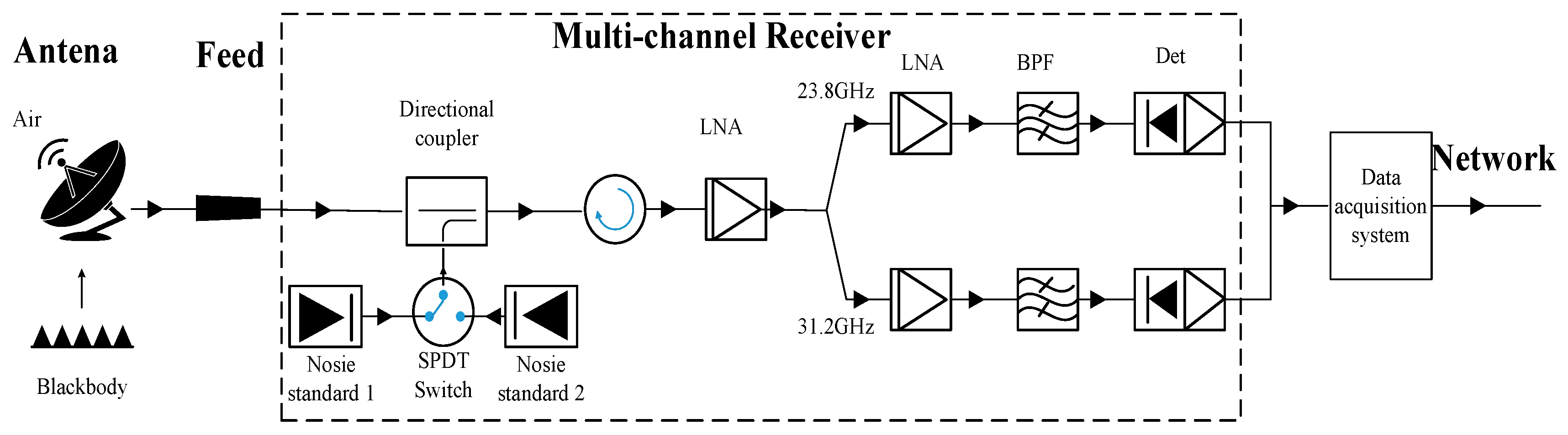
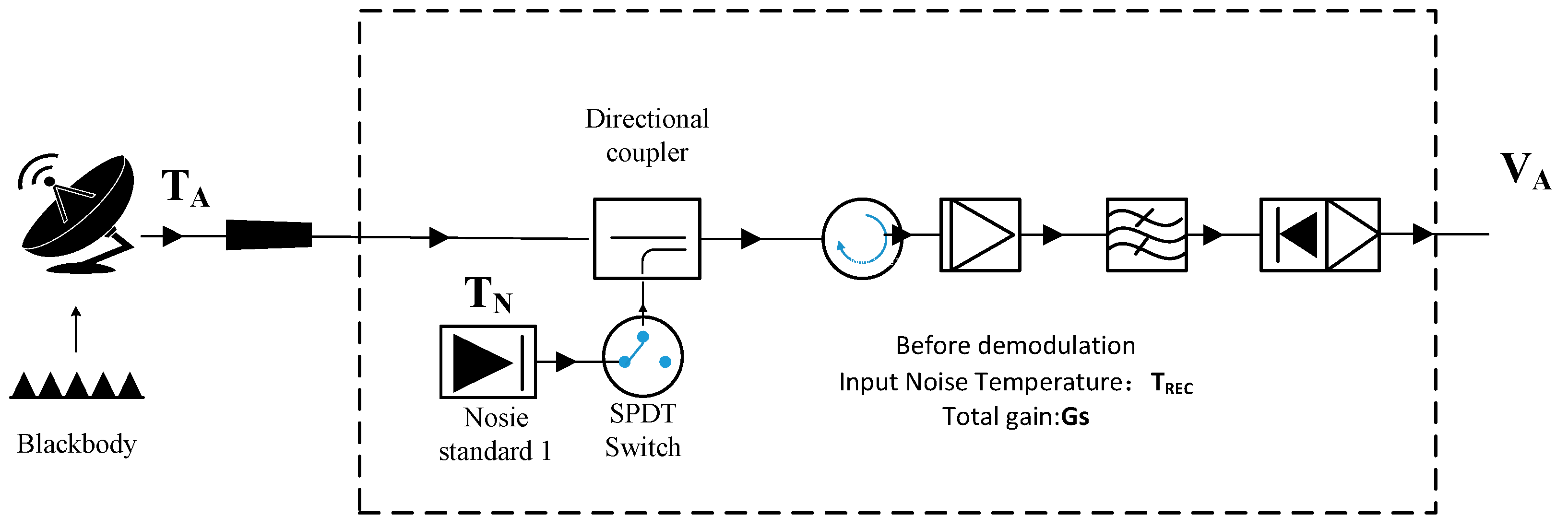
Modern radiometer designs include Robert Dicke and total power modes with a reference source to achieve calibration [6,7,8,9]. Figure 2 shows the schematic diagram of the HZD-X water vapor radiometer. It mainly includes an antenna feed system, receiving system, calibration blackbody, servo system, temperature control system, etc. The antenna system of the water vapor radiometer consists of a 0.8 m antenna and a feed. The multi-channel receiver sends the antenna output and synchronous gain correction noise source to the down-converter through the digital synthesis local oscillator for IF (intermediate frequency) processing and low-pass filtering, and finally converts the signal to its voltage value. The data acquisition system converts the measured voltage values into a sky brightness temperature and transmits them to the user through the network. The temperature control system is designed to ensure the stability of the receiver.
The specifications of the water vapor radiometer are shown in Table 1.
The schematic of the receiver system is shown in the dashed box in Figure 2. At the receiver input, the directional coupler allows for the injection of two precise noise signals generated by the single-pole double-throw (SPDT) switch. The two noise signals are used to determine the system noise temperature drift and system nonlinearity. Standard noise 1 has a temperature of approximately 300 K and standard noise 2 has a temperature of approximately 400 K. A low-noise amplifier (LNA) boosts the input signal before it is split into 16 branches, with only two being used for VLBI delay measurements. The splitter implements a waveguide bandpass filter (BPF), with the bandwidth and center frequency listed in Table 1.
The core concepts of the receiver design are as follows:
(1) The receiver design is centered on maximum thermal and electrical stability, compact layout, minimal connectors, and thermal drift elements;
(2) A temperature control system and air circulation system are added to ensure a constant temperature of 45 ± 0.05 degrees Celsius, which is the key to achieve a temperature accuracy of 0.2 K absolute brightness;
(3) Even after taking various measures, the measurement accuracy of the receiver will inevitably vary with the environment and other factors. Therefore, it is important to analyze and compensate for errors;
(4) When clouds cross the field of view, the wet delay is a rapidly changing quantity. Therefore, the receiver is designed to measure multiple channels in one second.
3. Error Source Analysis and Calibration
The WVR brightness temperature measurement error and the WVR inversion error contribute the most to the standard deviation of the wet path delay difference measured by the water vapor radiometer. Any error in the WVR instrument translates into a brightness temperature error and then into a wet path delay error. The calibration of the WVR for this project consists of the following four steps:
(1) Absolute system calibration is performed once a month, which includes the tip curve procedure discussed below;
(2) Receiver gain error calibration is performed. Noise standard temperatures are applied to calibrate receiver gain fluctuations in conventional radiometer observations;
(3) The temperature noise error of the antenna system is calibrated;
(4) Oblique path calibration is performed.
In the following, we analyze the different errors and their calibration results by experimental data.
3.1. Absolute Calibrations
It takes approximately 30 min for the system to reach temperature control after each re-energization. With a stable temperature, it is necessary to calibrate the entire system once a month, or, preferably, before each mission. The overall calibration can eliminate most of the errors of the radiometer hardware system at one time. The water vapor radiometer mainly uses an improved dumping method developed independently. Liquid nitrogen calibration, which can be performed in any weather, was not selected because the antenna was too large to design a convenient and feasible source of liquid nitrogen calibration. Tipping calibration is an important technique for the absolute calibration of ground-based microwave radiometers [1]. A new tilt calibration method for ground-based microwave radiometers has been improved to eliminate the radiation from cloudy liquid water and to effectively calibrate the radiometers under cloudy sky conditions. Since the inclination calibration part has been published in [10], we will not go into details here. Through extensive testing, we have verified the absolute calibration accuracy of the water vapor radiometer. The accuracy of the brightness temperature measurement can reach 0.2 K, even when the calibration is performed on a cloudy day.
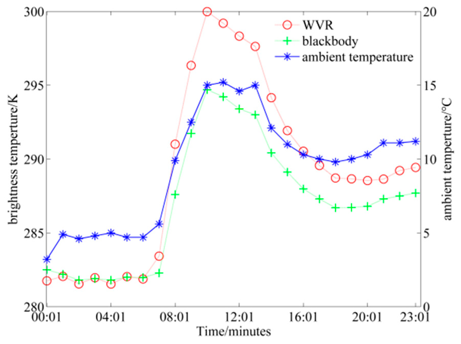
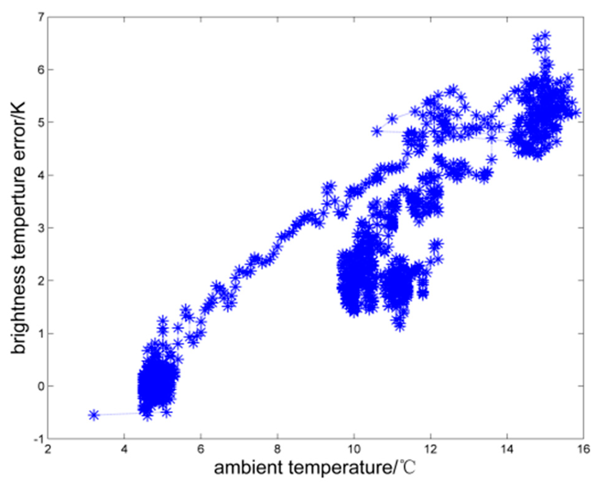
Since the absolute calibration can only guarantee the accuracy for a short time after the calibration is completed, in order to ensure a long-term stable measurement accuracy, the influence of the receiver gain, antenna system, and environmental factors must be considered. The following is a set of data. Tipping calibration was performed on the evening of 4 March 2017, followed by a 15-day observation experiment. The object observed on March 5 was a black body at room temperature, which was used to determine the accuracy of the brightness temperature measurement during the day. As shown in Figure 3, the brightness temperature measured by the water vapor radiometer deviated from the measured blackbody brightness temperature when the ambient temperature changed. As can be seen from the figure, the difference between the measured value and the theoretical true value is quite small (approximately 0.2 K) when observing the blackbody reference source from early morning to 7:00 a.m., but, after 7:00 a.m., as the sun rises (change in ambient temperature), the measured value gradually deviates from the theoretical true value, reaching a maximum value of 6 K at 9:30 a.m., and then the error gradually decreases. Figure 4 shows the relationship between the measurement error and the ambient temperature, and shows a clear correlation. Thus, the measurement error of the brightness temperature increases with the change in ambient temperature. The reason is that the change in ambient temperature will lead to fluctuations in the receiver gain and an increase in the antenna noise temperature. Later, we will discuss the errors caused by these cases and the approaches to eliminate them.
3.2. Receiver Gain Error Calibration
The effect of gain fluctuations on the stability of water vapor radiometers is direct and decisive. The water vapor radiation brightness temperature is usually tens of Kelvin. The total gain of the amplification link of the radiometer receiver is often more than 80 dB. In long-term operation, the gain fluctuation can easily exceed 1 dB. Therefore, the gain drift on the radiometer stability is very obvious, and must be suppressed in some way. The receiver gain drift is mainly caused by active devices (amplifiers and mixers), and active devices are mainly caused by changes in the ambient temperature. Gain drift with temperature (referred to as temperature drift) is an inherent characteristic of active devices and a key issue in RF circuit design. The receiver module of modern radiometers is usually placed in a constant temperature structure to ensure the stability of the amplifier’s ambient temperature. Despite this, the receiver gain can still drift, resulting in 1 K level errors. Periodic correction methods are needed in order to reduce the drift error.
Noise injection correction is currently a commonly used method, where noise power provided by a highly stable noise source is coupled to the antenna channel, and noise injection is controlled by the RF switch. This correction can be performed automatically at any time, so the gain fluctuation of the receiver can be corrected in real time. The noise injection radiometer is shown in Figure 5.
During measurement, the RF switch is periodically switched on and off to control the injection of noise.
(a) During the period when the noise source is turned off, the measurement equation is as follows:
where TA is the input radiation brightness temperature of the antenna port, TREC is the noise temperature of the system, GS is the total gain of the system, and VA is the output voltage value of the system after square-rate detection;
(b) During the period when the noise source is turned on, the measurement equation is as follows:
where TN is the temperature of the standard noise (reference noise), and VAN is the output voltage value of the system when adding noise.
Combining Equations (1) and (2), we obtain
VN is the output voltage of standard noise (reference noise), which can be obtained by subtracting the input voltage VA from the output voltage VAN.
The gain obtained by Equation (3) can be compared with the gain at the time of calibration to obtain the change in gain for correction in the final measurement results. This is a real-time gain correction method. From Equation (3), it can be seen that the accuracy of gain measurement depends on the stability of the noise source TN. Therefore, a high stability noise source is generally selected and placed in a constant temperature structure to maintain the stability of the noise output.
In practice, the gain of the receiving system and the input noise temperature will change. Assume that the gain of the system is GS0 and the noise temperature is TREC0 when the standard is just set. In the actual measurement, the gain of the system is GSi and the noise temperature is TRECi. According to Equation (3), the following equation can be obtained.
where VN0 is the input voltage of the reference noise source at the calibration time, and VNi is the input voltage of the reference noise source at the actual measurement time.
Then, we have the following,
Since the value of GS0 and TREC0 have been obtained and saved in the calibration, as long as the value of is obtained, the brightness temperature TAi at the measured voltage value of VAi can be computed. For convenience, the change in TREC is ignored here, i.e., assuming that , the estimated value of will be discussed in Section 3.3.
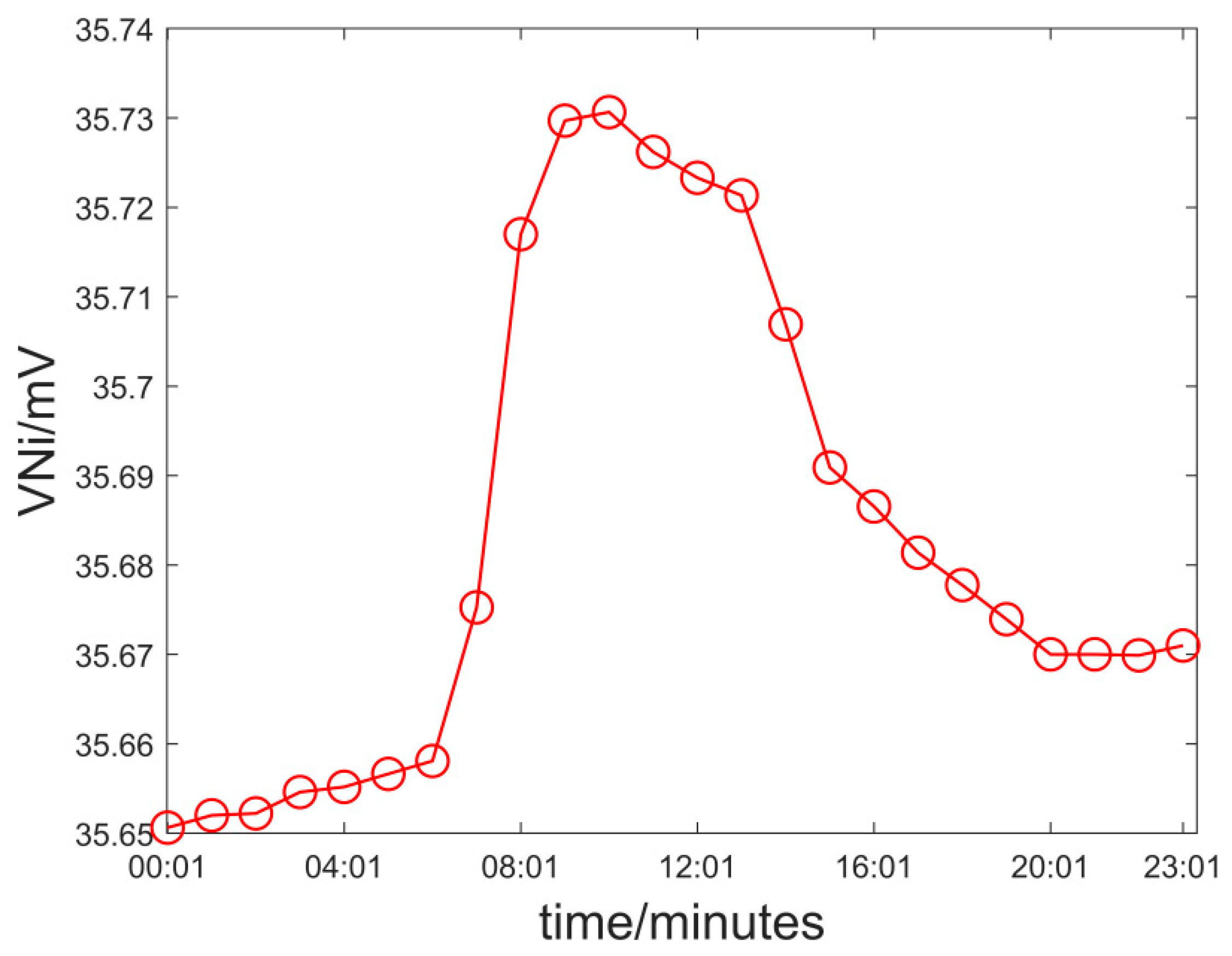
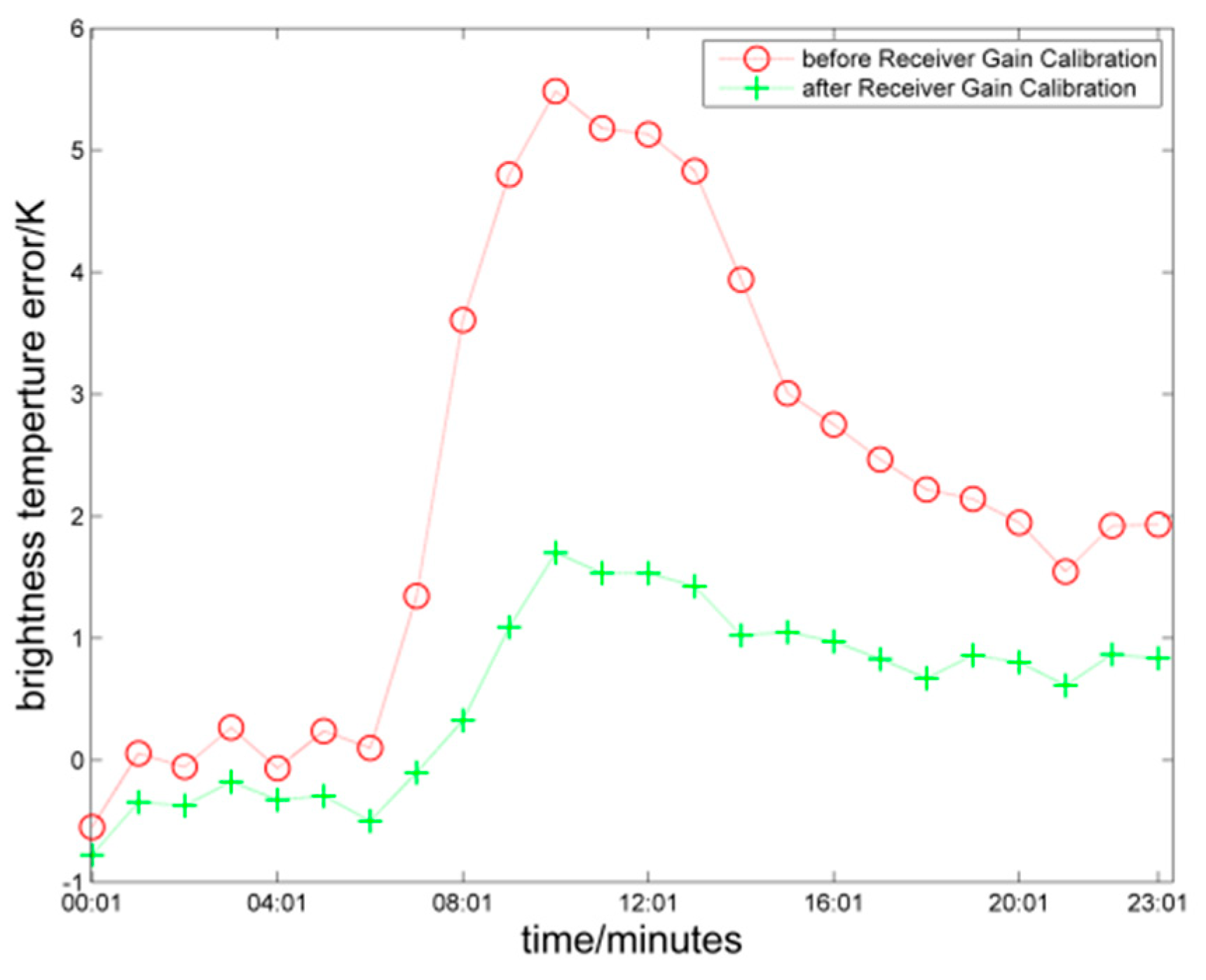
Figure 6 shows the variation of VNi on 5 March 2017. Figure 7 shows the measurement results of the blackbody after receiver gain error calibration. It can be seen from the figure that the error of measurement of the blackbody after receiver gain calibration is reduced by nearly 1 K at the maximum fluctuation of gain.
3.3. Temperature Noise Error of Antenna Feeder System
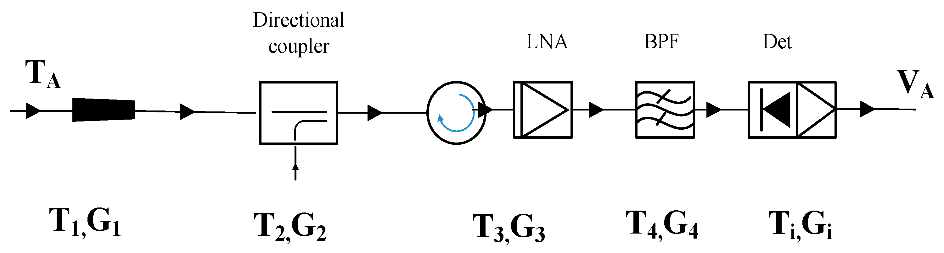
The following figure shows the noise error contribution of each component of the radiometer receiving system. The noise error after the antenna feeder can be compensated by the receiver gain error calibration method, as described in Section 3.2. However, since the noise source power enters the signal path after the feeding horn, it is impossible to correct the luminance temperature error introduced by the non-thermally stable feeding horn using the noise standard calibration method. An important system noise contribution is related to the antenna feed system. Figure 8 shows the noise contribution of each component of the WVR system. The system noise temperature converted to the input end is:
As shown in Figure 9, the noise temperature of the antenna T1 has a great impact on the noise temperature of the entire system, and the subsequent gain G is large enough. A typical loss of a waveform feedforward horn running at 20~30 GHz is less than L = 1 dB. When the physical temperature of the feedforward horn changes by 10 °C, the system noise increases by approximately 2 K, resulting in the absolute brightness temperature error of 2 K.
Therefore, the best way is to keep the antenna system at a constant temperature like the receiver. However, because the WVR antenna used in this project is large and exposed, it is difficult to keep the antenna at a constant temperature. Therefore, the temperature measurement probe can only be installed near the feeder in order to test the temperature variation of the antenna, thus eliminating this error.
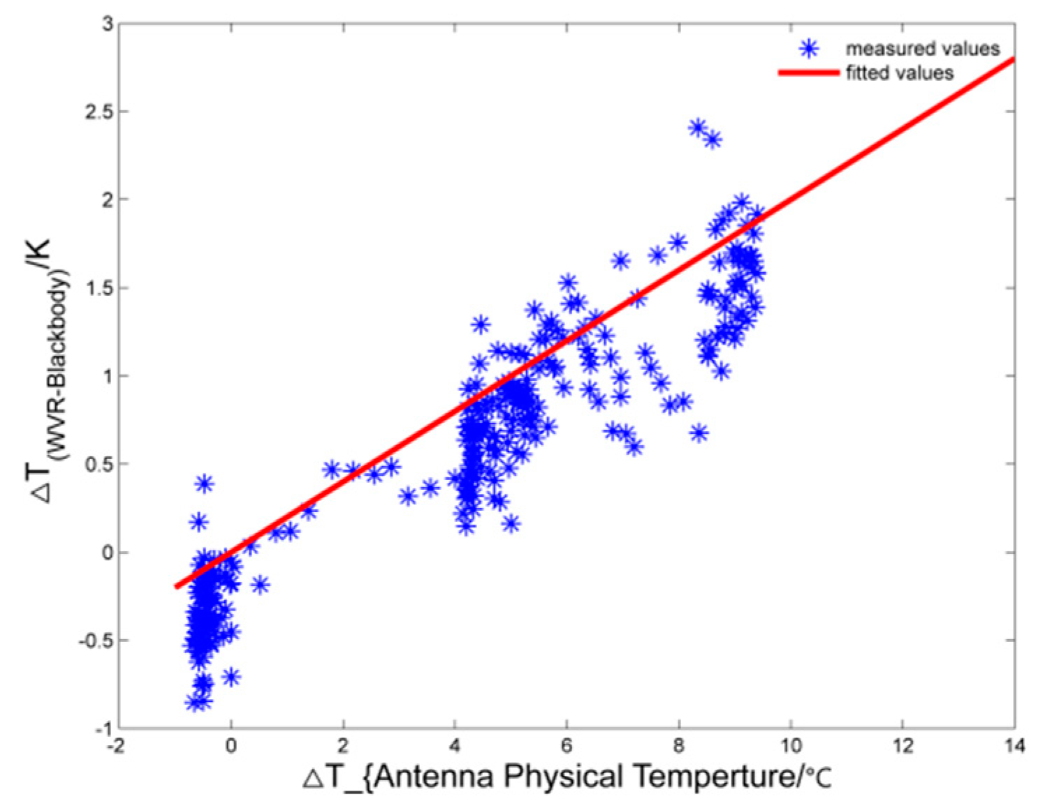
Figure 9 shows the relationship between the measured feed temperature and the difference between the measured WVR and the blackbody temperature. The measured values show that there is a clear linear relationship between them. By fitting a large number of measurements, the following relationship can be obtained:
∆Tf =Tw − TB= ∆T(APT) × 0.21
This relationship is very consistent with the previous analysis, where the measurement brightness temperature error of 2 K is caused by a 10 °C change in the feed temperature. Therefore, we need to add the error correction of the antenna and feeder to the final output brightness temperature. Combining Equations (5) and (6), the following equations can be obtained:
where TAi′ is the output bright temperature value data of the i-th group after correction of the antenna error, and is the measured physical temperature data at the feed source of the i-th group.
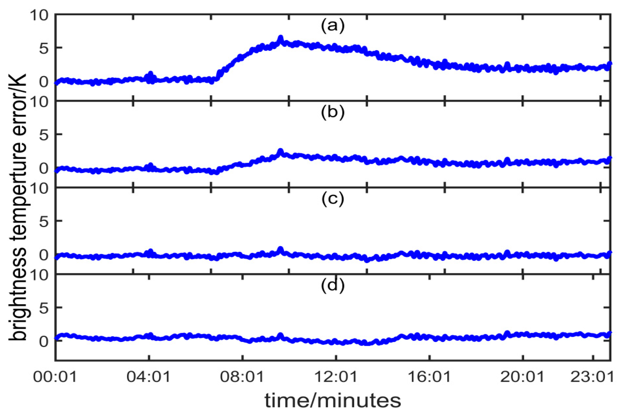
In summary, the measured data on 4 March 2017 were calibrated by using the three calibration methods described above. The results are shown in Figure 10, where Figure 10a shows the measurement error without calibration, Figure 10b shows the measurement error after system absolute calibration, Figure 10c shows the measurement error after receiver gain error calibration, and Figure 10d shows the measurement error after calibration of the temperature noise error of the antenna feeder system.
After the above three calibrations, the brightness temperature measurement accuracy of the vapor radiometer in the zenith direction can reach 0.2 K in a one-month scale (root mean square error) and 0.05 K in a 1000 s scale.
3.4. Oblique Path Calibration
As the measurement elevation angle decreases, the measurement accuracy of the microwave radiometer also decreases due to the effect of background noise on the main and side flaps of the antenna. There has been a challenge in evaluating the measurement accuracy of the microwave radiometer at low elevation angles and correcting the errors at low elevation angles. In this paper, based on the characteristics of atmospheric optical thickness, we investigate the optical thickness law calculated by using the brightness temperature measured by the microwave radiometer, and give an accurate evaluation of the measurement capability of the microwave radiometer at a low elevation angle indirectly.
According to the atmospheric transmission theory, the optical thickness of different zenith angles under clear weather is linearly related to the tangent of the zenith angle.
The optical thickness of each zenith angle can be computed as:
where is the average radiant light temperature of the atmosphere at elevation , and is the radiant light temperature of the sky at elevation and azimuth . The average radiant temperature of the atmosphere can be given by an empirical formula, and the radiant brightness temperature of the sky can be measured by a radiometer.
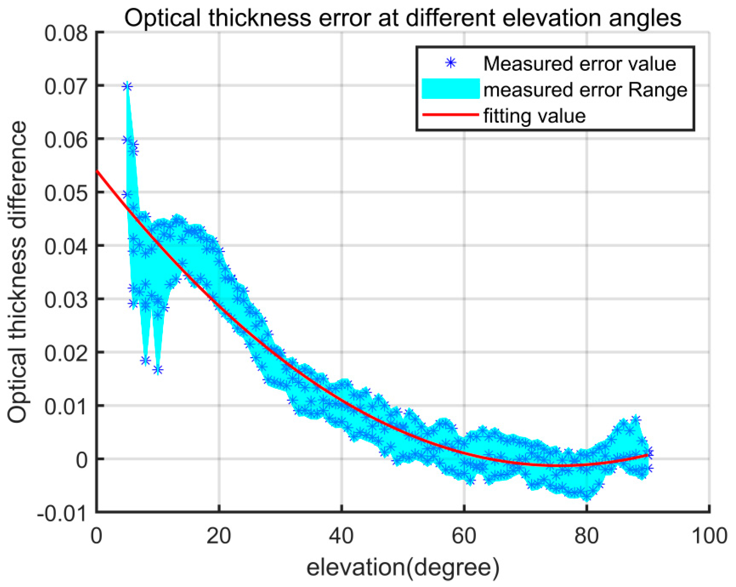
This is illustrated below by an observation experiment in April 2017 that was carried out in an open area with clear weather. In the experiment, an inclination calibration was first successfully performed, which ensured the accuracy of the brightness temperature data in the zenith direction. Figure 11 compares the measured optical thickness and the calculated theoretical optical thickness from an elevation angle of 5° to 90°. The measured optical thickness is measured by scanning the brightness temperature at different elevation angles and is calculated by Equation (8). The theoretical optical thickness is calculated from radiosonde data at the same address. From Figure 11, we found that:
(1) The measured optical thickness of the WVR is very close to the theoretical optical thickness when the elevation angle is greater than 60 degrees. Therefore, the brightness temperature measurements at elevation angles of 60–90 degrees are less influenced by external factors, such as sidelobes and the curvature of the Earth, without considering other factors. It can be considered that the measurement error is within an acceptable range;
(2) At elevation angles of 5 to 60 degrees, the smaller the variation of the optical thickness with elevation angle, the larger the deviation from the theoretical value. At an elevation angle of 10 to 60 degrees, the deviation has a certain relationship with the elevation angle, and the relationship can be fitted with a quadratic curve. At elevation 5 to 10 degrees, there seems to be little regularity in the deviation, which may be due to the influence of the ground feature.
Generally, when using WVR, VLBI uses data above 10 degrees. Therefore, in a practical measurement, we fit the law of optical thickness deviation by a large number of measured data, which can be used to correct the influence of the inclined path on the brightness temperature at an elevation angle of 10–90 degrees. By measuring the brightness temperature of different azimuths and elevations, we calculate and establish the measured optical thickness matrix, and then calculate the optical thickness deviation matrix. In this way, we can use the optical thickness deviation matrix to correct the brightness temperature values of different azimuths and elevations in the oblique path measurement, which greatly improves the brightness temperature measurement accuracy at lower elevations. The measurement airspace is divided into grids of 10 degree azimuth intervals and 1 degree pitch intervals, and the optical thickness deviation matrix is established as Equation (9), where represents the optical thickness deviation of the antenna pointing at azimuth angle and elevation angle . In general, VLBI uses data above 10 degrees when using WVR. Therefore, in the actual measurement, we fit the law of optical thickness deviation by a large amount of measured data, which can be used to correct the effect of the tilted path on the brightness temperature at elevation angles of 10–90 degrees. By measuring the brightness temperature at different azimuth and elevation angles, we calculate and build the measured optical thickness matrix, and then calculate the optical thickness deviation matrix. In this way, we can use the optical thickness deviation matrix to correct the brightness temperature values of different azimuth angles and elevations in the oblique path measurement, thus greatly improving the brightness temperature measurement accuracy at low elevations. The measurement airspace is divided into grids of 10 degree azimuth intervals and 1 degree pitch intervals, and the optical thickness deviation matrix is established as Equation (9), where represents the optical thickness deviation of the antenna pointing at azimuth angle and elevation angle . After the optical thickness at different elevation angles is measured, (the fitting value) can be obtained through binary primary regression.
According to Equation (12),
Then, we obtain,
where is the bright temperature after the correction of the oblique path, is the original bright temperature measured, and can be calculated through the empirical model.
After the step-by-step correction of the methods in Section 3.1, Section 3.2, Section 3.3 and Section 3.4, we have achieved an accuracy of 20 mm (10 degrees above elevation) of the oblique path wet delay measurement. The error comparison method uses a two-station VLBI system to measure two stars with known precise positions in order to obtain more accurate atmospheric delays by the difference method. The related experimental procedure and results will be discussed in the follow-up papers.
4. Conclusions
In this paper, we developed a water vapor radiometer for VLBI observations. We describe the details of the design of the water vapor radiometer, the sources of measurement errors, and the correction methods. By using the four error correction methods, the long-term measurement accuracy of the brightness temperature reaches 0.2 K, whereas the measurement accuracy of the wet delay is 15 mm (tilted path 20 mm). The water vapor radiometer satisfies the expected requirements of our project, but there is still a big gap compared with the experimental results of JPL. The AWVR brightness temperature measurement accuracy developed by JPL can reach 0.1 K, and the wet delay measurement accuracy can reach 1 mm. This excellent performance is mainly due to the design of the integrated receiving system, excellent thermostatic control system, and larger antenna (1.8 m), which can obtain a higher system sensitivity and can reduce the influence of the sidelobe. At the same time, the choice of measurement frequency is also an important factor. We use fewer measurement channels. In designing the next generation water vapor radiometer, more radiometer measurement channels will be added in order to obtain sufficient atmospheric radiation information. Future work will focus on the further improvement of hardware and an exploration of error calibration methods. We also observed that the measurement results are poorer in the case of more rain or clouds, which is mainly due to the influence of liquid water [11,12,13]. This work can be extended to select the optimal frequency and to further optimize the algorithm performance.
Author Contributions
Conceptualization, Z.Z.; Funding acquisition, Q.K.; Investigation, J.G.; Methodology, H.C. and Q.Z.; Project administration, Q.Z.; Software, H.C.; Supervision, J.G.; Validation, Q.K.; Writing—original draft, H.C.; Writing—review & editing, Z.Z. All authors have read and agreed to the published version of the manuscript.
Funding
This research received no external funding.
Institutional Review Board Statement
Not applicable.
Informed Consent Statement
Not applicable.
Data Availability Statement
Data set available on request to corresponding authors.
Acknowledgments
Thanks to Shanghai Astronomical Observatory, Chinese Academy of Sciences for their supports and suggestions in improving the stability of the water vapor radiometer.
Conflicts of Interest
The authors declare no conflict of interest.
References
- Bar-Sever, Y.; Jacobs, C.; Keihm, S.; Lanyi, G.; Naudet, C.; Rosenberger, H.; Runge, T.; Tanner, A.; Vigue-Rodi, Y. Atmospheric Media Calibration for the Deep Space Network. Proc. IEEE 2007, 95, 2180–2192. [Google Scholar] [CrossRef]
- Linfield, R.; Keihm, S.; Teitelbaum, L.; Walter, S.; Mahoney, M.; Treuhaft, R.; Skjerve, L. A test of water vapor radiometer-based troposphere calibration using very long baseline interferometry observations on a 21-km baseline. Radio Sci. 1996, 31, 129–146. [Google Scholar] [CrossRef]
- Keihm, S.J. Water Vapor Radiometer Measurements of the Tropospheric Delay Fluctuations at Goldstone over a Full Year. Available online: https://tmo.jpl.nasa.gov/progress_report/42-122/122J.pdf. (accessed on 25 November 2021).
- Morabito, D.D.; Addario, L.R.; Keihm, S.; Shambayati, S. Comparison of Dual Water Vapor Radiometer Differenced Path Delay Fluctuations and Site Test Interferometer Phase Delay Fluctuations Over a Shared 250-Meter Baseline. Interplanet. Netw. Prog. Rep. 2012, 42, 188. [Google Scholar]
- Morabito, D.; D’Addario, L.; Acosta, R.; Nessel, J. Tropospheric delay statistics measured by two site test interferometers at Goldstone, California. Radio Sci. 2013, 48, 729–738. [Google Scholar] [CrossRef]
- Pei-yuan, X. Chinese Dual Frequency Water Vapor Radiometer for VLBI; Symposium—International Astronomical Union: Paris, France, 1988; Volume 129, p. 549. [Google Scholar]
- Tanner, A.; Riley, A. Design and performance of a high-stability water vapor radiometer. Radio Sci. 2003, 38, 15-1–15-11. [Google Scholar] [CrossRef]
- Beckman, B. A Water-Vapor Radiometer Error Model. IEEE Trans. Geosci. Remote Sens. 1985, GE-23, 474–478. [Google Scholar] [CrossRef]
- Williamson, E.; Houghton, J. A Radiometer-Sonde for Observing Emission from Atmospheric Water Vapor. Appl. Opt. 1966, 5, 377. [Google Scholar] [CrossRef]
- Li, J.; Guo, L.; Lin, L.; Zhao, Y.; Cheng, X. A New Method of Tipping Calibration for Ground-Based Microwave Radiometer in Cloudy Atmosphere. IEEE Trans. Geosci. Remote Sens. 2014, 52, 5506–5513. [Google Scholar]
- Wu, S.-C. Optimum frequencies of a passive microwave radiometer for tropospheric path-length correction. IEEE Trans. Antennas Propag. 1979, 27, 233–239. [Google Scholar]
- Brown, S. A Novel Near-Land Radiometer Wet Path-Delay Retrieval Algorithm: Application to the Jason-2/OSTM Advanced Microwave Radiometer. IEEE Trans. Geosci. Remote Sens. 2010, 48, 1986–1992. [Google Scholar] [CrossRef]
- Crewell, S.; Czekala, H.; Löhnert, U.; Simmer, C.; Rose, T.; Zimmermann, R.; Zimmermann, R. Microwave Radiometer for Cloud Carthography: A 22-channel ground-based microwave radiometer for atmospheric research. Radio Sci. 2001, 36, 621–638. [Google Scholar] [CrossRef]
Figure 1.
WVR next to the Shanghai Tianma telescope.

Figure 2.
The schematic diagram of the HZD-X water vapor radiometer.

Figure 3.
The brightness temperature of the water vapor radiometer at 23.8 GHz frequency and the brightness temperature of the black body were measured when the ambient temperature changed.
Figure 3.
The brightness temperature of the water vapor radiometer at 23.8 GHz frequency and the brightness temperature of the black body were measured when the ambient temperature changed.

Figure 4.
The relationship between measurement error and ambient temperature.

Figure 5.
Block diagram of noise injection radiometer system.

Figure 6.
VNi changes on 5 March 2017.

Figure 7.
The error of measuring blackbody after receiver gain error calibration was reduced by nearly 1 K.
Figure 7.
The error of measuring blackbody after receiver gain error calibration was reduced by nearly 1 K.

Figure 8.
Contribution of WVR components of system noise temperature TREC.

Figure 9.
The relationship between the measured feed temperature and the difference between the measured WVR and the blackbody temperature.
Figure 9.
The relationship between the measured feed temperature and the difference between the measured WVR and the blackbody temperature.

Figure 10.
Calibration results of the measured data on 4 March 2017. (a) shows the measurement error without calibration, (b) shows the measurement error after system absolute calibration, (c) shows the measurement error after receiver gain error calibration, and (d) shows the measurement error after calibration of the temperature noise error of the antenna feeder system.

Figure 11.
The optical thickness error at different elevation angles.


Table 1.
Key radiometer specifications.
| Parameter | Specifications |
|---|---|
| Operating Frequency | 23.8 GHz, 31.2 GHZ |
| channels | 2 |
| IF Bandwidth | 100 MHz |
| Antenna Sidelobe Level | −27 dB |
| Calibrated Brightness Temperature Accuracy | 0.2 K |
| Measurement Resolution | 0.05 K |
| Operating Temperature Range | −50 to 65 deg C |
| Mass | 200 kg |
Publisher’s Note: MDPI stays neutral with regard to jurisdictional claims in published maps and institutional affiliations. |
© 2021 by the authors. Licensee MDPI, Basel, Switzerland. This article is an open access article distributed under the terms and conditions of the Creative Commons Attribution (CC BY) license (https://creativecommons.org/licenses/by/4.0/).
Share and Cite
MDPI and ACS Style
Chen, H.; Ge, J.; Kong, Q.; Zhao, Z.; Zhu, Q. Error Correction of Water Vapor Radiometers for VLBI Observations in Deep-Space Networks. Atmosphere 2021, 12, 1601. https://0-doi-org.brum.beds.ac.uk/10.3390/atmos12121601
AMA Style
Chen H, Ge J, Kong Q, Zhao Z, Zhu Q. Error Correction of Water Vapor Radiometers for VLBI Observations in Deep-Space Networks. Atmosphere. 2021; 12(12):1601. https://0-doi-org.brum.beds.ac.uk/10.3390/atmos12121601
Chicago/Turabian StyleChen, Houcai, Junxiang Ge, Qingde Kong, Zhenwei Zhao, and Qinglin Zhu. 2021. "Error Correction of Water Vapor Radiometers for VLBI Observations in Deep-Space Networks" Atmosphere 12, no. 12: 1601. https://0-doi-org.brum.beds.ac.uk/10.3390/atmos12121601
Note that from the first issue of 2016, this journal uses article numbers instead of page numbers. See further details here.