
Characteristics and Long-Term Variability of Occurrences of Storm Surges in the Baltic Sea


1
Institute of Marine and Environmental Sciences, University of Szczecin, 70-383 Szczecin, Poland
2
Faculty of Navigation, Maritime University of Szczecin, 70-500 Szczecin, Poland
*
Author to whom correspondence should be addressed.
Atmosphere 2021, 12(12), 1679; https://0-doi-org.brum.beds.ac.uk/10.3390/atmos12121679
Submission received: 28 October 2021
/
Revised: 8 December 2021
/
Accepted: 12 December 2021
/
Published: 14 December 2021
(This article belongs to the Special Issue Water Environment of Coastal Areas under Current and Future Climate)
Abstract
:Understanding the characteristics of storm surges is especially important in the context of ongoing climate changes, which often lead to catastrophic events in the coastal zones of seas and oceans. For this reason, this paper presents the characteristics of the Baltic Sea storm surges and trends in their occurrences through the past 60 years. The study material was based on hourly sea level readings, spanning the years 1961–2020, retrieved from 45 Baltic Sea tide gauges, as well as air pressure and wind field data. Owing to the analysis and visualization of storm situations, two main types of storm surges were identified and characterized: a surge driven by wind and a surge driven by subpressure associated with an active low pressure area. This paper also discusses a third, mixed type of storm surge. Further analyses have indicated that through the past 60 years in the Baltic Sea, the duration of high sea level has increased by 1/3, the average number of storm surges has increased from 3.1 to 5.5 per year, and the maximum annual sea levels have increased—with a trend value of 0.28 cm/year. These processes, also observed in other marine basins, provide strong evidence for contemporary climate change.
1. Introduction
Currently, the Baltic Sea has many rationally-located tide gauges (about 220 mareographs along the entire Baltic coast). Owing to this, the phenomena and processes involved in raising and lowering sea levels can be thoroughly characterized. Especially important are extreme sea levels which have reached their highest and lowest levels in many years, in a given year, or during a given storm event. These extremes stimulate current processes, marine abrasion, and accumulation of sedimentary material along different sections of the coastal zone. High sea levels, which are usually generated under stormy conditions, often lead to catastrophic situations, such as beach erosion, as well as destruction of shore infrastructure. Storm surges may lead to flooding of low-lying areas, which are typically densely populated, and may result in heavy economic losses. The study of storm surges has practical aspects and enables the maritime administration to determine warning levels, develop flood prevention services, protect coastal areas, as well as ensure the safety of shipping and operation of ports.
Understanding storm surge characteristics is especially important in the context of ongoing climate changes. Studies from the previous 20 years and the latest 6th IPCC Report [1] clearly point to a continued rise of mean and maximum sea levels, increasing wind velocity, and the resultant increase in intensity, frequency, and catastrophic character of storm phenomena. This knowledge is essential for coastal zone management and developing local spatial management plans by local administration.
The present study aims to characterize storm surges based on two main types of surges that occurred in 2020 in the Baltic Sea. The focus of the latter part of the paper is on showing trends in occurrences of storm surges and extreme sea levels on the Baltic Sea coasts over the past 60 years.
Storm surges on the coasts of the Baltic Sea, as in northwestern Europe, are most often generated by the passage of low pressure systems along with accompanying atmospheric fronts [2]. Storm surges depend on three components [3]:
- the filling-up of the Baltic Sea—the initial sea level prior to the occurrence of an extreme event. (Water exchange between the North Sea and the Baltic Sea, accomplished via the Danish Straits, is the main driver of changes in water volume and the average sea level—that is, the filling of the basin. This exchange depends on local wind and pressure conditions over the North Atlantic and the Baltic Sea and on the North Sea water level [4]. The largest inflows of water into the Baltic Sea occur during extended periods characterized by sustained western winds, which lead to the filling-up of the Baltic Sea and suppress water outflow. This may lead the Baltic Sea to rise up to several tens of centimeters above mean sea level [2])
- the action of tangential wind stresses within the given area (wind directions: whether they are shore- or seaward, wind velocities, and the duration of wind action),
- the deformation of the sea surface by mesoscale deep low-pressure systems rapidly crossing the Baltic Sea, which produces a water cushion (baric wave) and generates seiche-like variations of the Baltic Sea level. A water cushion is a surge of water caused by subpressure associated with a low-pressure system, resulting from the inverse barometer effect (a 1 hPa drop in pressure in the depression center increases the sea level by 1 cm).
The most important features of a low-pressure system that determine whether a deformation will occur are: the pressure in the center, the trajectory, and the velocity. Due to the interactions between these three factors, extremely high sea levels may occur during the positive storm surge phase (sea level rise), while extremely low levels may occur during the negative phase (sea level fall).
Although the Baltic Sea is not a large body of water, storm surges occurring there are quite large. The surge in the Gulf of Finland on 19 November 1824 generated the highest sea levels ever recorded in the Baltic Sea. In the area of St. Petersburg, the sea level reached 4.21 m above the tide gauge zero [5]. The Gulf of Riga, along with the Pärnu Bay and areas adjacent to the west coast of Estonia, frequently experience high sea levels (over 2 m above the zero of a tide gauge) and dangerous storm surges. This issue is addressed in many works by Suursaar and colleagues [6,7,8]. The largest surge ever recorded on the southwestern coast of the Baltic occurred on 13 November 1872 [9]. In many Western Baltic ports, this surge exceeded 3 m above the tide gauge zero (Schleswig 3.49 m, Travemünde 3.30 m, Schleimünde 3.21 m) and resulted in extensive floods, large shoreline losses, and many fatalities. Significant storm surges and extreme sea levels (1.40 m above the tide gauge zero) also occur on the Polish coast, and the shores of the shallow Pomeranian Bay are particularly vulnerable, since surges can damage dunes and cliffs [10]. High surges have also occurred in the northern Gulf of Bothnia (the tide gauge in Kemi indicated a maximum of 2.01 m above the gauge zero). In the rest of the Baltic Sea, storm surges are lower [5].
The present study is a continuation of previous analyses performed by the authors, addressing many aspects of storm surges and extreme water level occurrences in the Baltic Sea [11,12,13]. A new aspect of the present study is the identification and characterization of the types of storm surges depending on the prevailing causal factor: wind or subpressure of an active low-pressure area. Another new aspect is the analysis of the longest obtainable sea level data series, spanning 1960–2020, and using these to determine trends in multi-year variability in storm surges and extreme sea levels.
2. Materials and Methods
2.1. Research Material
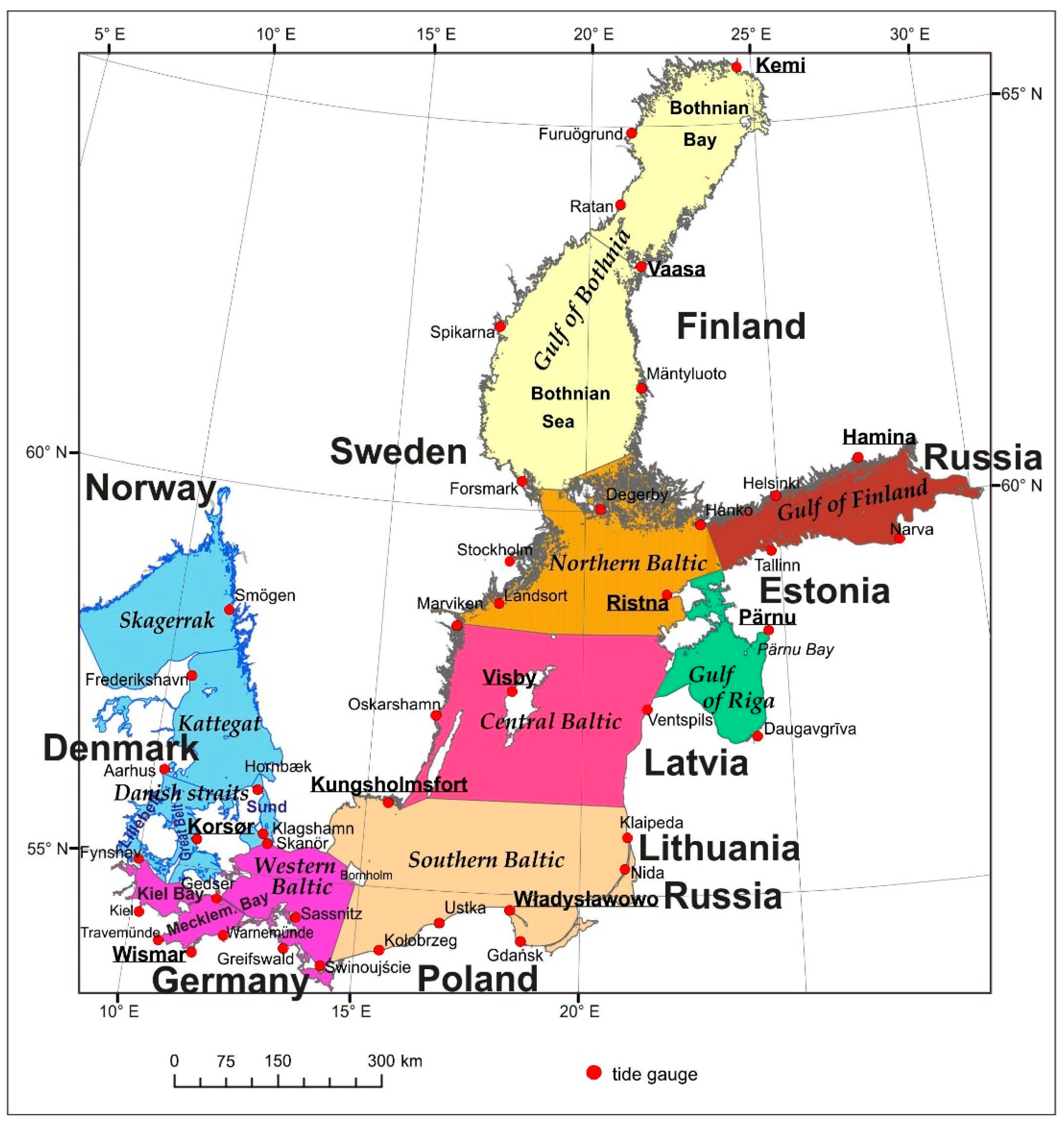
The research material included hourly sea level observation data from 45 tide gauges located along the Baltic Sea coasts from the period 1960 to 2020 (Figure 1). This 61-year period is the longest series of hourly sea level observations available in the resources of the national hydrological and meteorological institutes of the Baltic States. Hourly sea level values were referenced to the zero of the local tide gauge, the vertical datum of which is based on the Mean Sea Level (MSL). Data from all 45 tide gauging stations were utilized for visualization of short-term Baltic Sea surface changes during storm surges (Figure 1). However, 10 tide gauge stations were selected for the analyses of trends in the occurrences of storm surges and extreme sea levels. At these 10 stations, the recorded sea level fluctuations display a similar course to other stations within the particular sub-basins of the Baltic Sea. For this reason, the following 10 stations were deemed representative of trends in their respective Baltic Sea sub-basins: Korsør (Danish Straits, Great Belt), Wismar (Western Baltic), Kungsholmsfort and Władysławowo (Southern Baltic), Visby (Central Baltic), Pärnu (Gulf of Riga), Hamina (Gulf of Finland), Ristna (Northern Baltic), Vaasa (middle part of the Gulf of Bothnia), and Kemi (northern part of the Gulf of Bothnia—Bothnian Bay). This division of the Baltic Sea into sub-basins is based on the results of the authors’ earlier work—Wolski and Wiśniewski [12] (Figure 1).
2.2. Description of the Storm Event
The paper describes the two storm events which occurred between 13 and 16 October 2020 and between 20 and 23 November 2020. As part of this description, the following features of the low pressure system together with storm event parameters were listed for several tide gauge stations located in different places of the Baltic coast:
- pi—pressure at the center of the low pressure area (hPa),
- VL—average speed of the low pressure area (m/s),
- initial sea level (cm) (the sea level prior to the occurrence of an extreme event),
- extreme values of the sea level (maximum and minimum level) during the surge and their amplitude (cm),
- rates of the maximum sea-level rise and fall (cm/h),
- duration of ≥70 cm and ≥100 cm sea levels and ≤−70 cm and ≤−100 cm sea levels (relative to tide gauge zero).
Additionally, for each analyzed storm situation, we determined sea level variability along with wind direction and velocity, and plotted the trajectory of the low-pressure system. Such detailed analysis of a given storm situation, and the utilization of two boundary values characterizing the low-pressure area (pressure at the center, 980 hPa, and velocity, 16 m/s) enabled us to distinguish two types of storm surges. For details see Section 3.1.
2.3. Visualization of Changes in the Baltic Sea Surface during a Storm Situation in ArcGIS
ArcGIS was the basic tool for visualizing changes in the Baltic Sea surface during a storm situation. The advantage of GIS software is that it links analyzed research features with their precise geographical locations. Spatial analysis was primarily based on an ArcGIS module called kriging, which is widely used and recommended for environmental research, including the creation of maps based on data interpolation [14]. Kriging is a geostatistical method used to interpolate parameter values. In a broader sense, it is used to estimate continuous surfaces (maps of expected value) by point-wise measurements of quantitative data. The weighted average over a subset of adjacent points is used to obtain a specific interpolation point using the formula [15]:
where:
Z*(x0)—interpolated value at x0,
Z(xi)—actual value at the measurement point (sea level at a given tide gauging station),
wi—kriging weight, and
n—number of points considered in kriging (12 for analyses in the present paper).
The main advantage of using kriging for the spatial analyses in this paper is that isoline maps prepared following this method reveal clear trends in the differentiation of the examined parameters. There is no such effect for maps created with, e.g., inverse-distance gridding, in which it is more difficult to see regularities [15].
2.4. Research on Trends of Extreme Sea Levels and Storm Surges
In the present study, trends in the occurrence of storm surges and extreme sea levels for the period 1960–2020 were determined. To determine the number of storm surges with maximum sea levels ≥70 cm above local tide gauge zero for particular years, we adopted the definition of a storm surge by Wolski et al. [11]. In addition to storm trends, trends in the duration (number of hours) of high sea levels, i.e., levels ≥70 cm relative to tide gauge zero, were also determined. Definition of the high sea levels was based on warning water levels used by hydrological surveys of the Baltic States during periods of storm flood threat. For most of the Baltic coast, the warning level (so-called high water) was higher than 70 cm [16,17,18]. The third analysis concerned the trends in the height of maximum annual sea levels. In all long-term trend analyses, the linear regression method was used. Calculations were made at the statistically significant level α = 0.05.
3. Results and Discussion
3.1. Types of Storm Surges in the Baltic Sea
The Baltic Sea is a tideless and semi-enclosed sea. During storm situations lasting 10–20 h and several days, the sea surface table displays a considerable increase in some sub-basins, and a concomitant significant decrease in other sub-basins. The applications of ArcGIS to visualize the Baltic Sea level readings based on MSL enables a precise imaging of sea surface deformation. Owing to the visualization, we analyzed storm situations in order to identify distinct types of storm surges depending on their driving mechanisms. Additionally, we considered the degree of the Baltic Sea sub-basin filling, and the features of the respective low-pressure systems: progressive velocity, pressure at the system center, migration track, and wind velocities, directions, and duration. As a result, two main types of storm surges were recognized: wind-driven surge and subpressure-driven surge.
- A wind-driven storm surge occurs when over the course of several days, a wind field exerts an influence on the sea surface, with stable wind direction and high wind velocity causing evident drift currents. Such wind field may arise in the case of shallow and slow-moving low-pressure systems (pressure at the center >980 hPa, velocity <16 m/s). Tangential wind action not only produces waves but also contributes energy to the formation of a sloping water surface, so-called wind-driven surge. The magnitude of sea level surge or sea level lowering depends not only on wind velocity, but also on its duration, direction, wind distances over sea surface, and compensating currents in the coastal zone.
- A subpressure-driven storm surge occurs when a mesoscale, concentric, and deep (≤980 hPa at the center) low-pressure area moves at relatively high velocity (≥16 m/s) over or in close proximity to the Baltic Sea. This causes a deformation to the Baltic Sea surface via the so-called water cushion of a low pressure area, which moves in an oscillatory manner along the low-pressure area trajectory and the adjacent sub-basins. A water cushion, also termed a baric wave, is a surge of water caused by subpressure (just like ocean waters surge underneath a tropical cyclone). Such inverse barometer effect over the sea surface is characterized by positive ordinates in the central area and negative ordinates along the deformation periphery. If a baric wave moves at a velocity equal to or approximating the progressive velocity of the low-pressure area, a serious flooding hazard occurs at a given section of the coast, and so-called seiche-like oscillations may arise.
In reality, during every storm surge, there is synchronous activity of wind (tangential force) and pressure field (mesoscale low-pressure area moving over the Baltic Sea). It is important to determine which factor (wind or subpressure) has a considerably higher contribution, and if this is impossible, both factors need to be considered equally important. Such case can be considered as the third storm surge type—a mixed surge (subpressure–wind surge).
3.1.1. Wind-Driven Storm Surge Example
The first example is a wind-driven storm surge in the Western Baltic, accompanied by an expanded stationary high-pressure system over the North Atlantic and a shallow low-pressure area over Central Europe.
Synoptic Situation
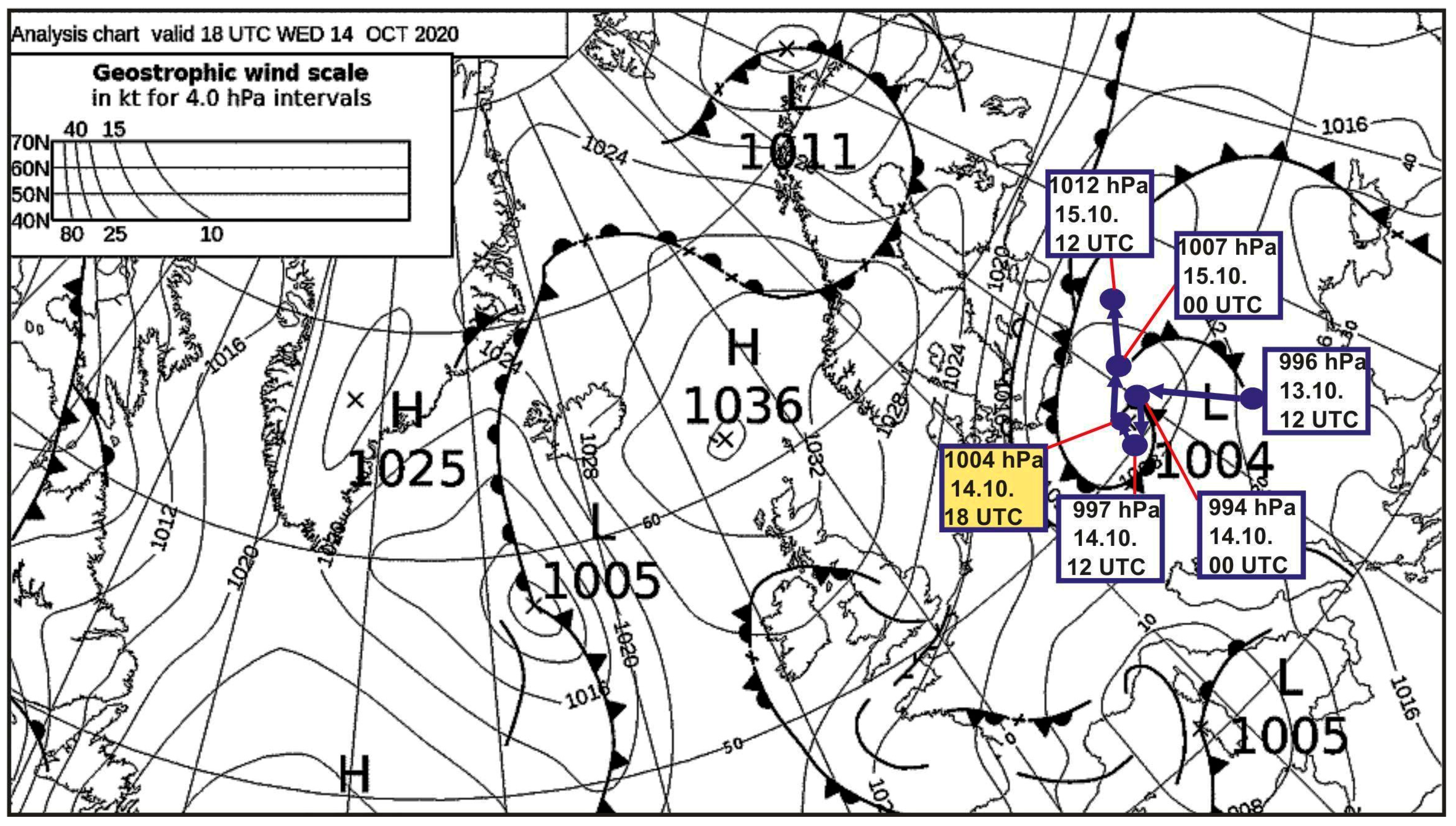
From the afternoon of 13 October to 16 October, the Baltic Sea was under the influence of an expanded stationary high-pressure system centered north of the British Isles. This high-pressure system covered the North Sea, the Norwegian Sea, and large parts of both the Scandinavian Peninsula and the Baltic Sea. Air pressure within the center of this high-pressure area equaled about 1036 hPa. At the same, a shallow (994–1012 hPa) low-pressure area resided over Central Europe (Figure 2), which was slowly moving (at about 8 m/s) toward the northeast, underneath the high-pressure system. The low gradually weakened until it disappeared on 16 October 2020. Additionally, on 14 and 15 October 2020, an occluded front, associated with a shallow low-pressure area (1011 hPa) centered above the Barents Sea, was passing over the northern part of the Scandinavian Peninsula and the northern Gulf of Bothnia. This synoptic situation caused a high pressure gradient, and conditions enabling an intensive inflow of air masses from the northeast over the majority of the Baltic Sea sub-basins from 13 to 16 October 2020 (Figure 2).
Western Baltic
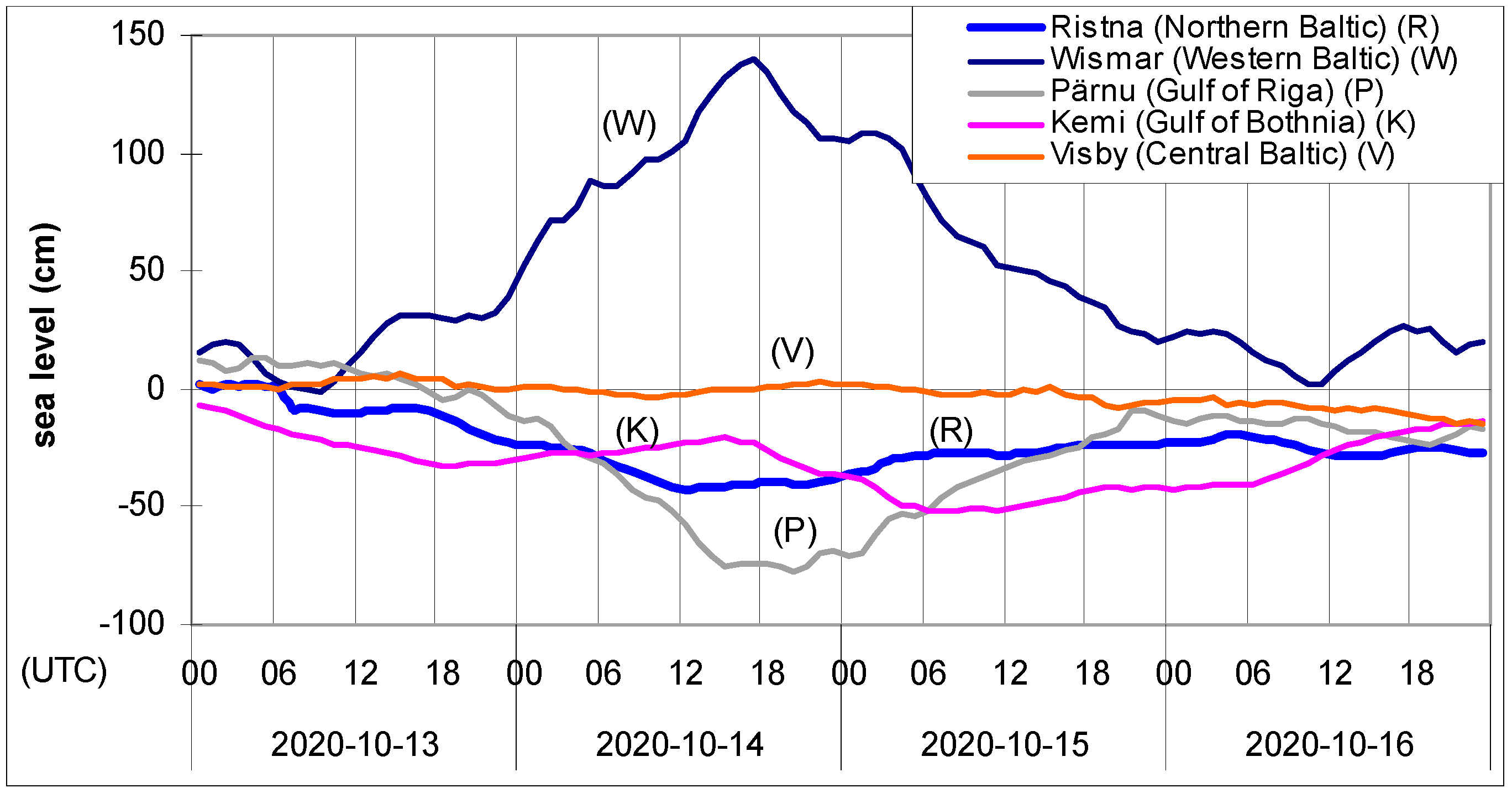
From noon on 13 October, stations located in the western Baltic Sea recorded a clear, uniform sea level rise that lasted over 24 h, until the evening of 14 October (Figure 3 and Figure 4). This stable increase was accompanied by a strong, onshore wind blowing from the northeast at velocities exceeding 10 m/s. The wind accelerated on 14 October, up to 20 m/s in Świnoujście and 14 m/s in Wismar, when a shallow (1004 hPa), but rather extensive low-pressure area started moving from over Central Europe toward the Southern Baltic coast, creating a high pressure gradient (Figure 2). In Świnoujście, the maximum sea level recorded was +110 cm (14.00 UTC, 14 October), in Skanör +84 cm (15.00 UTC), and in Wismar +140 cm (17.00 UTC) (Table 1). It was a typical wind-driven surge resulting from an onshore wind, and it was associated with the filling-up of shallow bays of the Western Baltic. For two consecutive days, until the afternoon of 16 October, tide gauging stations in this sub-basin showed a sea level decrease down to the average level, at a maximum rate of 9–11 cm/h. The Western Baltic sea level lowering was accompanied by decreasing wind velocity and low-pressure area disappearance (Figure 2 and Figure 4).
Danish Straits
The Korsør tide gauging station located within the Great Belt recorded similar sea level variability compared to the neighboring Western Baltic tide gauging stations, at identical wind conditions (strong wind blowing at 10–12 m/s from the northeast) (Figure 4). One factor causing slight modification to sea level variability was the presence of tides. The maximum sea level at this station equaled 69 cm, and was attained at 22.00 UTC on 14 October. The impact exerted by the northeastern wind caused the water table to slope from the south toward the north of the Danish Straits, and thus favored an outflow of waters from the Baltic Sea to the North Sea (Figure 5).
Southern Baltic
Sea level oscillations in the Southern Baltic Sea were consistent with the Western Baltic, but no storm height was reached. The station at Kungsholmfort attained a maximum sea level of just 47 cm (10.00 UTC, 14 October) while a weaker and partly offshore northeastern wind was blowing at up to 11 m/s (Figure 4).
Central and Northern Baltic
With a northeastern wind blowing at 4–9 m/s, the Central Baltic sea level oscillated within the range of average sea levels. Wind direction at Visby was parallel to the coast and thus did not cause the sea level to either rise or drop. The Northern Baltic tide gauging stations recorded moderate and low water levels associated with northern and northeastern, moderate and weak wind blowing at <5 m/s. In such conditions, with offshore wind, the station at Ristna recorded a minimum sea level of −42 cm on 14 October at 13.00 UTC (Table 1). Sea levels remained low in the Northern Baltic over the subsequent days, until 16 October (Figure 3 and Figure 4).
The Gulf of Finland and the Gulf of Riga
Sea level variability and wind characteristics within the Gulf of Finland and the Gulf of Riga were highly similar to analogous processes in the Northern Baltic. Tide gauging stations recorded moderate and low water levels accompanied by a weak and moderate, but stable, northeastern wind (below 6 m/s). The minimum sea level was lower than in the Northern Baltic, equaling −50 in Hamina (the Gulf of Finland, 18.00 UTC, 14.10.). A minimum sea level value of −77 cm was recorded in the Gulf of Riga (Pärnu station, 20.00 UTC, 14.10.). The sea level in the Gulf of Finland and the Gulf of Riga remained low (below tide gauge zero) until the end of the storm on 16 October, accompanied by northeastern air mass circulation (Figure 3 and Figure 4).
The Gulf of Bothnia
Between 13 and 16 October 2020, the Gulf of Bothnia witnessed a changing, northeastern, western, and northwestern wind, the variability in wind direction being caused by a migration over this sub-basin of an occluded front associated with a shallow low-pressure area (1011 hPa), centered over the Barents Sea. For the Kemi Station (on the Bay of Bothnia), the prevalent wind blew at 6–8 m/s from northerly directions. Such offshore wind conditions resulted in average and low sea levels (−52 cm, 6.00 UTC, 15 October) that lasted throughout the four-day period until 16 October 2020 (Figure 3 and Figure 4).
Wind-Driven Storm Surge Event—A Summary
The discussed storm situation is an example of a storm surge arising due to the influence of a northeastern air mass inflow over the Baltic Sea sub-basins. This is a rare case of a storm surge in the Western Baltic that resulted from a strong wind arising from a high pressure gradient between an expanded high-pressure area (1036 hPa, North Atlantic) and a shallow low-pressure system (994–1012 hPa) that formed over land (Central Europe). Areas located at the junction of these two extensive systems, i.e., the Western Baltic with shallow bays: the Bay of Mecklenburg, the Bay of Wismar, and the Bay of Kiel, and also—in part—the Southern Baltic, experienced the influence of strong and very strong wind (wind velocities up to 20 m/s), from the northeastern wind field. This wind, via drift currents, lowered the water surface in the northern and eastern Baltic sub-basins, and raised the water surface in the western sub-basins (water mass transfer). This denivelation of the Baltic Sea surface is visible on instantaneous sea level maps (Figure 5). The Western Baltic storm surge culmination took place on 14 October 2020 (at 17.00 UTC). Maps for 15 and 16 October display the process of regaining sea level balance in the Baltic Sea (Figure 5).
The high sea level (≥70 cm) persisted over a significant number of hours, which also points to a wind-driven origin of the discussed surge event. For the Western Baltic, ≥100 cm sea level lasted on average 18 h and ≥70 cm—for 30 h (Wismar) (Table 1). The remaining Baltic Sea sub-basins, Central and Northern Baltic, Gulfs of Riga, Finland and Bothnia, as well as Skagerrak and Kattegat, were located within the range of an expanded high-pressure area from over the North Atlantic, and recorded only moderate and low water levels.
3.1.2. An Example of a Storm Situation with the Main Part Played by the Subpressure of an Active Low-Pressure Area
This example focuses on the influence of a dynamic deep low-pressure area migrating over the Atlantic and the Norwegian Sea, and causing seiche-like Baltic Sea level oscillations.
Synoptic Situation
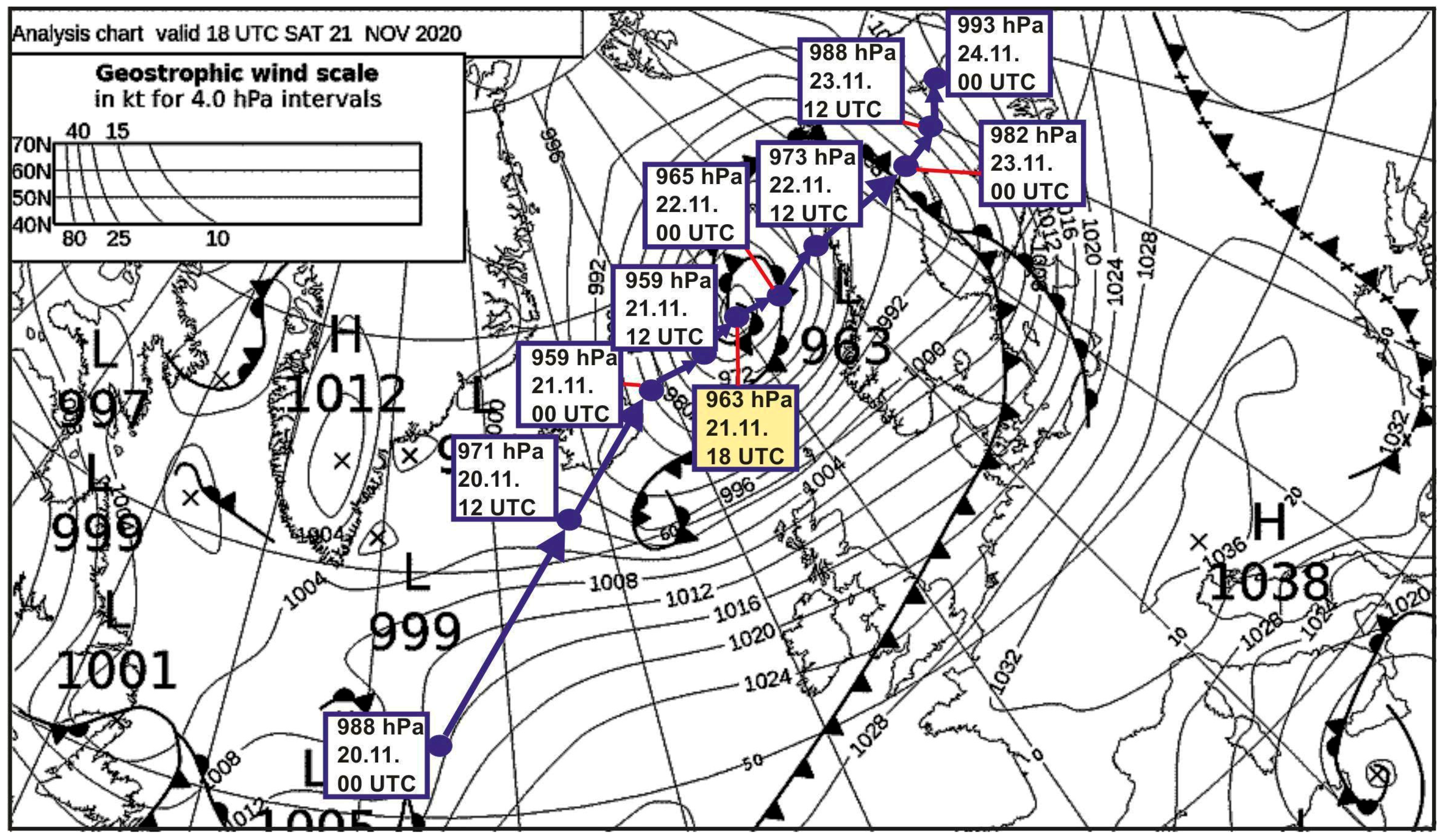
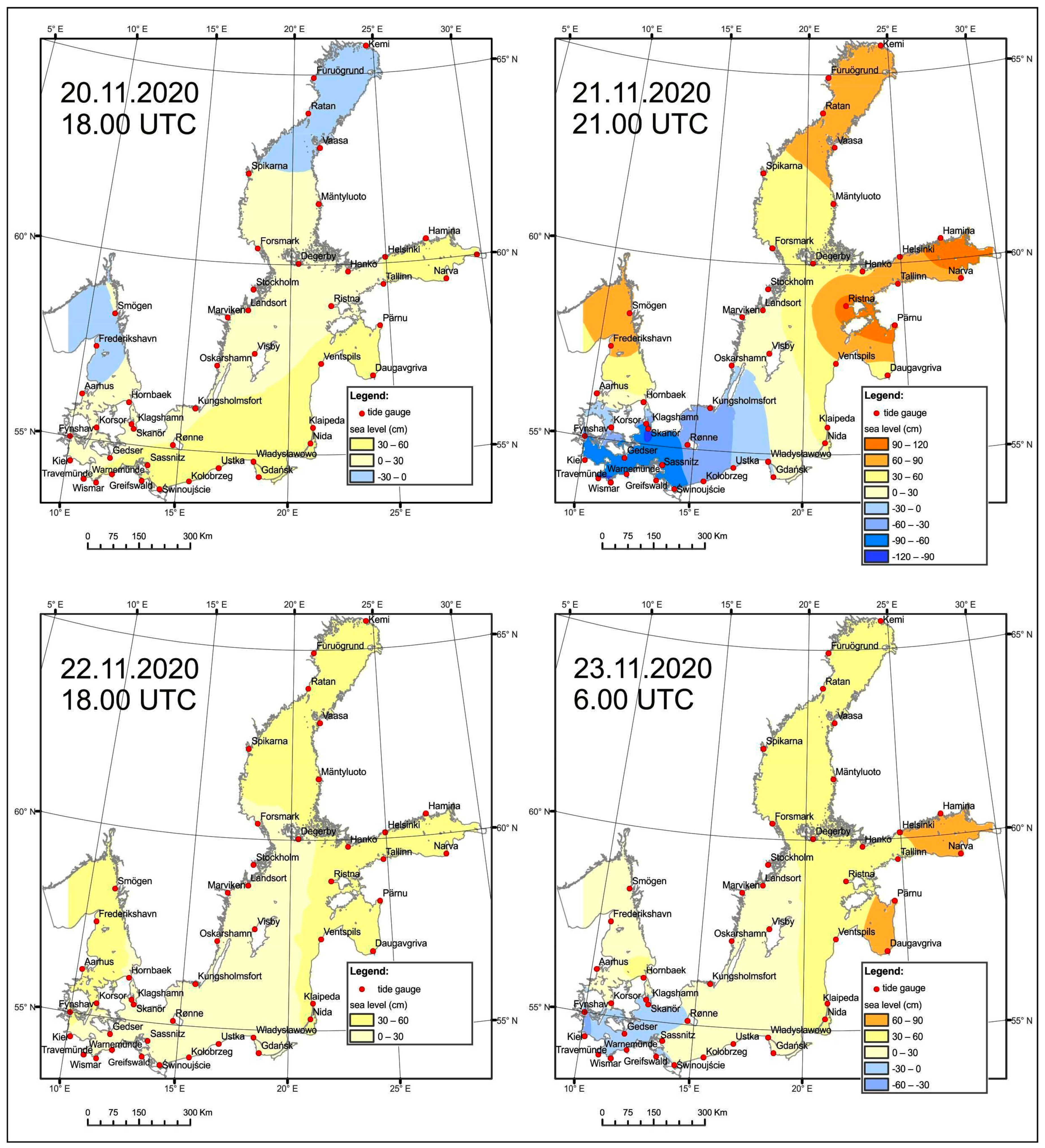
On 20 November 2020, a 988 hPa low-pressure area moved from the North Atlantic (south of Greenland) over the Norwegian Sea (east of Iceland), where it deepened to 959 hPa in the center (00:00 UTC, 21 November). During this time (i.e., 20 November), the Baltic Sea was within the range of an extensive high-pressure wedge centered over Central Germany (1037 hPa, 18.00 UTC, 20 November). On 21 November, the center of the low pressure area from east Iceland migrated further east toward the Scandinavian Peninsula (963 hPa, 18.00 UTC, 21 November). On this day, the low-pressure area occupied the entire Baltic Sea and Northern Europe. The entire continental Europe, however, remained under the influence of a high-pressure system (Figure 6). The subsequent 48 h (22–23 November 2020) was a period of further migration of the low-pressure area eastward over the Scandinavian Peninsula and the Bay of Bothnia toward the White Sea. During this time, the air pressure within the depression rose to 993 hPa. The eastward migration of this deep low-pressure area over a high-pressure system blocking it from the south, caused strong southwestern and western winds over the Baltic Sea basin, and seiche-like sea level oscillations within the entire Baltic Sea basin.
Western Baltic
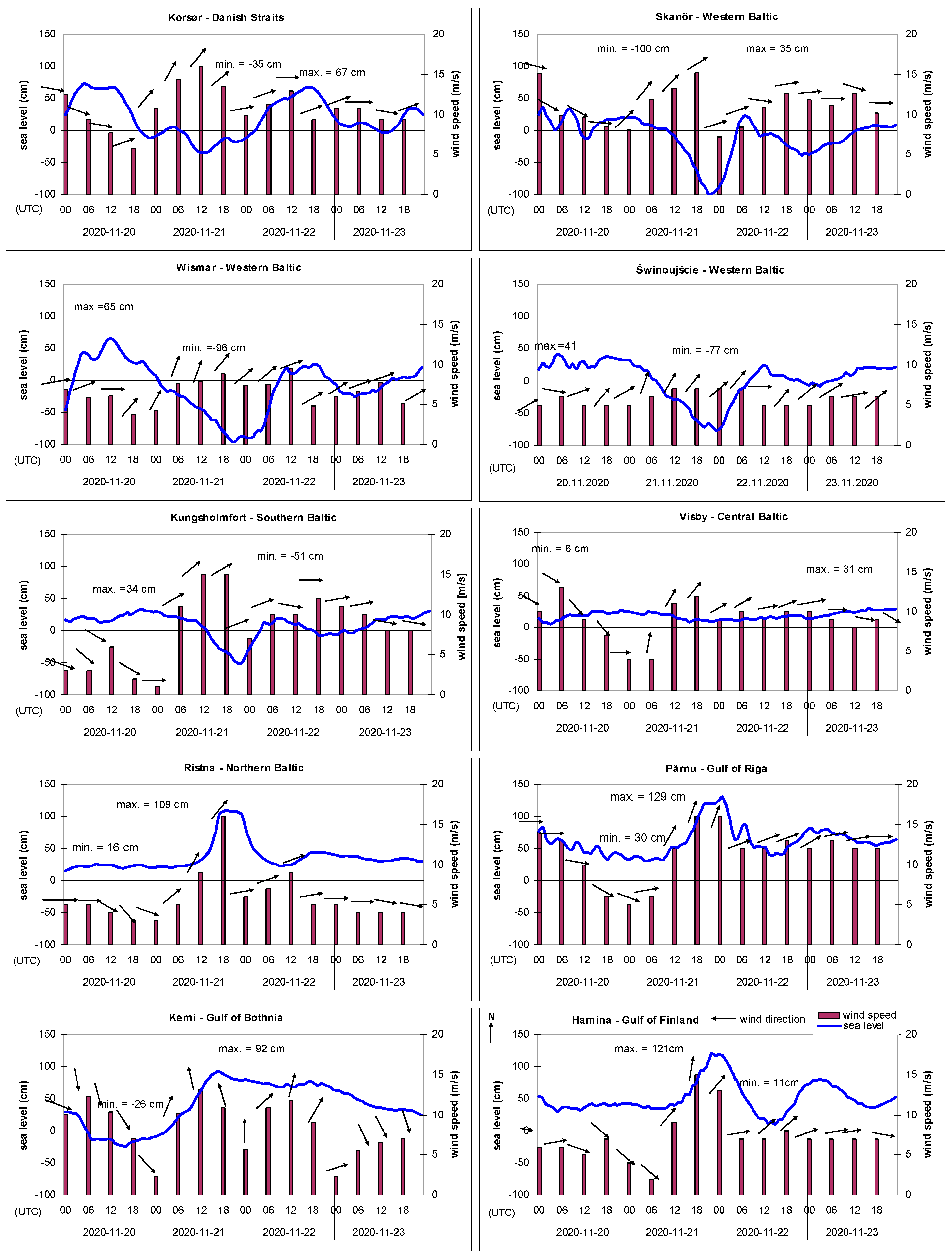
From the afternoon of 20 November 2020, tide gauging stations in the Western Baltic Sea recorded decreasing sea levels, with a maximum rate of 11–19 cm/h. This decrease was initially accompanied by a wind blowing from the western and southwestern sector, at moderate velocities (below 10 m/s). On 21 November, when the center of the Norwegian Sea low-pressure area reached its extreme values (959–963 hPa) (Figure 6), the Western Baltic tide gauging stations recorded their sea level minima. The Wismar station recorded −96 cm (21.00 UTC, 21 November), the Skänor station –100 cm (22.00 UTC, 21 November), and the Świnoujście station −77 cm (23.00 UTC, 21 November) (Table 2, Figure 7 and Figure 8). This was the negative storm surge phase, associated with the influence of the subpressure of the active depression centered over the Norwegian Sea. From 00 to 06 UTC on the following day, 22 November, tide gauging stations in the Western Baltic recorded dynamically increasing sea levels, which rose until mean states were attained, despite sustained offshore winds blowing from the southwest (Figure 8—Skänor, Wismar and Świnoujście stations. These winds only delayed a rapid sea level rise that was mostly caused by the subpressure of an active low-pressure area. This marked the onset of Baltic surface deformation phase change from negative to positive, accompanied by the eastward migration of the low-pressure area. Once the maximum was attained, the Western Baltic sea level started decreasing again, but the minima reached on 23 November were not as deep, because the center of the low-pressure area moved over land, and it ceased to exert a strong influence on sea surface (Figure 7 and Figure 8).
Danish Straits
At Korsør station located within the Great Belt, the sea level variability was coherent with the sea surface deformation recorded in the Western Baltic (Wismar station). The negative phase of the surge, however, was not as deep, and equaled −35 cm (13.00 UTC, 21 November). The positive phase, however, was more distinct at Korsør than at the Wismar station and reached a maximum of 67 cm (12.00 UTC, 22 November), accompanied by a wind characteristic similar to that for the Western Baltic (Figure 8).
Southern Baltic
At the Kungsholmsfort station, sea level variability was similar to the Western Baltic. The minimum sea level of −51 cm was attained on 21 November at 21.00 UTC (Figure 8).
Northern and Central Baltic
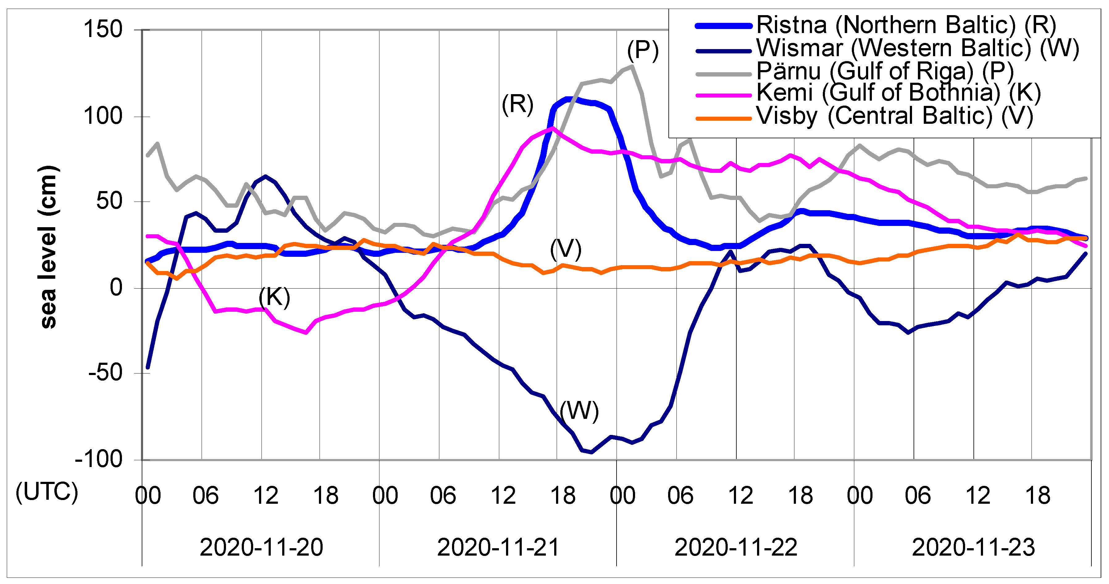
During the negative sea surface deformation phase in the Western Baltic, a concomitant positive storm surge phase occurred in the Northern Baltic Sea (Figure 7). Tide gauging stations in the Northern Baltic recorded their maxima synchronously with sea level minima in the Western Baltic, at similar wind characteristics (southwestern wind). The station at Ristna noted a maximum sea level of +109 cm (19.00 UTC, 21 November). The maximum rate of sea level increase at this station equaled 26 cm/h and was the highest in the entire Baltic Sea. The Visby station, however, located in the Central Baltic Sea (Gotland), recorded moderate sea levels (Figure 8), despite strong winds blowing throughout the duration of the storm situation.
The Gulf of Finland and the Gulf of Riga
Water level variability in the Gulf of Finland and the Gulf of Riga was similar to the Northern Baltic situation. Only the positive storm surge phase was noted in both sub-basins (Figure 7 and Figure 8). The main water level maxima reached during this phase were higher than in the Northern Baltic due to the high filling-up (initial level): 50 cm for the Gulf of Finland and 78 cm for the Gulf of Riga (Table 2). In Hamina (Gulf of Finland), a maximum of +121 cm was recorded (22.00 UTC, 21 November), while in Pärnu (Gulf of Riga), the maximum equaled +129 cm (1.00, UTC, 22 November. On the following days, 22 and 23 November, the sea levels displayed a considerable drop followed by an increase at both tide gauging stations (Figure 8), despite stable onshore southwestern winds. This points to a less important part played by the wind, and suggests a dominant part played by the subpressure associated with the active and deep low-pressure area in shaping this storm situation instead.
The Gulf of Bothnia
In the Gulf of Bothnia, the course of the storm surge was only partly similar to the Northern Baltic. The main surge maximum at the Kemi station (+92 cm at 17.00 UTC, 21 November) matched the positive phase of the surface deformation in the Northern Baltic (Figure 7). In Kemi, the water levels remained high (>70 cm) for 28 h, until 23 November. This was caused by the close proximity of the track of the baric depression. Its center was passing over the northern part of the Scandinavian Peninsula and the northern Gulf of Bothnia. The subpressure and wind field associated with this depression sustained high sea levels at the Kemi station (Figure 8).
Storm Surge Driven by Subpressure of an Active Low-Pressure System—A Summary
During the November 2020 surge, the dynamic changes to the Baltic Sea surface that took place over the course of 24 h, cannot be explained solely by the wind field characteristics. Strong sea level drops and rises occurred while the wind was stable, moderate (below 8 m/s), and blew continuously from the southwest, for instance at the Western Baltic stations at Wismar, Skänor, and Świnoujście (21/22 November), or at the Hamina station within the Gulf of Finland on 22–23 November (Figure 8).
On the other hand, a strong wind blowing at >10 m/s caused no sea level extremes in the Central Baltic (the station at Visby) (Figure 7 and Figure 8). This hydrologic situation was mostly influenced by subpressure associated with a deep and active low pressure system, with its negative and positive phase (the Baltic Sea surface deformation via the so-called baric wave, i.e., a water cushion underneath the depression). The negative storm surge phase occurred clearly only in the Western and Southern Baltic, and partly within the Danish Straits. Only the positive storm surge phase occurred in the northern and eastern Baltic Sea sub-basins (Northern Baltic, the Gulf of Finland, the Gulf of Riga, and the Gulf of Bothnia). This was influenced by the direction and the track of the low pressure system. A characteristic feature of this particular surge was the creation of a peculiar sea surface slope between the northeastern sub-basins (Northern Baltic, the Gulf of Finland, the Gulf of Riga), and the Western Baltic together with the Danish Straits. The degree of the slope changed as the storm surge progressed. The highest sea surface slope occurred during the negative phase culmination in the Western Baltic, and the concomitant positive phase culmination in the northeastern sub-basins. These contradictory high and low water level variations are apparent from 18.00 UTC on 21 November to 1.00 UTC on 22 November (Figure 7). Within this period, the highest variations were recorded at the stations located in the distalmost parts of the Baltic Sea: Wismar, Pärnu, Ristna, and Kemi, and the difference in slope exceeded 2 m. Characteristically, for seiche-like oscillations, the station at Visby, located on the island of Gotland in the central part of the Baltic Sea, displayed minimum oscillations due to its position at the nodal line of a seiche.
This particular storm situation may be regarded as a classic case of so-called Baltic seiche caused by a dynamic and deep low pressure system. Clear seiche oscillations of the Baltic Sea are convincingly shown on the instantaneous sea level maps from 20 to 23 November 2020 (Figure 9). Dynamic, deep low-pressure area at the same time lowers the sea level in the south and in the west, and raises the sea level in the north and in the east, following which, in a matter of hours, it reverses the Baltic Sea water table slope. Wind made little impact on this storm surge. In fact, the effect of the wind was restricted to delaying the sea level increase in the Western Baltic and decelerating the sea level drops at the northeastern Baltic coasts.
3.1.3. Characteristic Features of Storm Surges in the Baltic Sea
Based on the analysis of the storm events included in this work and based on previous analysis many other storm situations a number of features may be identified as characteristic of subpressure- and wind-driven storm surges.
Storm situations generated by subpressure of a dynamic low-pressure system are characterized by:
- An active mechanism of dynamic inclination of the sea level from the balance state via a mesoscale low pressure system moving at a velocity of about 16 m/s and higher; its activity causes a deformation to the Baltic Sea surface via the so-called water cushion (baric wave) and oscillatory fashion of the propagation of such deformation along the track of the low pressure area and the adjacent sub-basins;
- A characteristic phenomenon of alternating sea level oscillations between southwestern and northeastern sub-basins of the Baltic Sea. A mesoscale depression simultaneously lowers the sea level in the south and raises the sea level in the north, following which, in a matter of hours, the Baltic Sea surface table slope becomes reversed. Such water mass movements can be termed seiche oscillations of the entire Baltic Sea.
- Wind has no high significance for subpressure-driven storm surges and may at most contribute to sustaining a extreme sea level;
- Storm surges generated by subpressure associated with a low pressure area begin with a large sea level decrease at tide gauging stations in the Western Baltic;
- The narrow range of sea level oscillations (20–50 cm) at the Visby station (Central Baltic) during storm situations corroborates that this tide gauge is located on the nodal line of a Baltic seiche;
- In the case of surges caused by a dynamic low-pressure area, the maximum rate of sea level change equals on average from 10 to 40 cm/h or more. The fastest sea level rises and drops occur at tide gauges located within bays and straits.
Wind-driven storm situations are characterized by the following features:
- Wind-driven surges last relatively long (48 to 72 h); during this time, drift currents transfer water mass, thus forming a so-called coastal wind surge.
- The maximum rate of sea level change is usually lower than in the case of surges caused by a dynamic low-pressure area and equals on average from 5 to 25 cm/h. Notably, however, the rate of sea level drop is usually slightly slower than the rate of increase (gravity- driven decrease).
- In the case of eastern or northern atmospheric circulation, and the presence of an expanded anticiclonic system over Scandinavia or western Russia, storm surges occur only in southwestern sub-basins of the Baltic Sea. In such cases, tide gauging stations located within these sub-basins do not record a sea level drop (i.e., there is no negative phase of the surge).
- When a maximum sea level is attained during a wind-driven surge at a given tide gauging station, wind direction exerts a stronger forcing than wind velocity. A weaker wind blowing more perpendicular relative to the coast will cause a higher wind-driven surge and will cause the maximum to be attained sooner than in the case of a stronger wind blowing at a lower angle relative to the coast.
The dominant wind factor in the origin of a storm surge is well described in the majority of studies concerning the dynamics of the Baltic Sea waters [5,6,7,8,10,19,20,21,22,23]. According to Sztobryn et al. [10] and Tisel [20], strong onshore winds blowing from the northwestern to northeastern sector, arising after the passage of an atmospheric front, are responsible for storm surges in the southwestern Baltic Sea. The wind direction change zone, significant for the water level rise or drop, in such cases moves generally along with the migration of the low-pressure area [10,20,21]. In studies by Suursaar et al. [6,7,8], Jaagus i Suursaar [24] indicated that the highest sea levels reached at Estonian coasts are associated with deep low-pressure areas forming strong southwestern and western winds, blowing at appropriate angles relative to the coastal bays.
According to the authors of the present paper, this dominant contribution of the wind factor in shaping storm surges is clear in the case of a slow migration of a depression, when the coastal zone remains exposed to gusty winds for a long time. When a deep low-pressure area (<980 hPa) moves at high velocity (≥16 m/s), however, the time of wind forcing in a given direction is restricted [25]. In such conditions, tangential impact exerted by the wind on a basin surface alone does not lead to extreme sea level values ranging from −2 m in the Western Baltic to over +3 m at the northeastern coasts of the Baltic Sea. In such cases, winds may only act to sustain these extremely low or extremely high sea levels [3,11,25,26]. It is therefore necessary to include sea surface deformation by subpressure of a rapidly moving depression, in considerations of storm surge origin.
This factor is still underestimated in the literature, which has a negative impact on explaining the mechanisms driving extreme events, such as coastal zone floods or excessively low sea levels posing a threat to the safety of shipping. So-called dynamic sea surface deformation and seiche oscillations occur due to a progressive movement of a low-pressure area over the sea surface. Such deformation may become larger with higher velocity of the low-pressure system migration [3,25,27,28]. Averkiev and Klevany [5] found that the most dangerous storm surges in the Gulf of Bothnia and the Gulf of Finland are generated by dynamic baric depressions moving at velocities >14 m/s toward the northeast or east–northeast.
3.2. Changes in High Sea Levels and Storm Surges from 1960 to 2020
The discussion on high sea level and storm surge variability through the period spanning 1960–2020 is based on an analysis of trends displayed by the duration of high sea levels (≥70 cm relative to tide gauge zero), and trends in the number of storm surges per year. Another analysis is to identify trends in the long-term course of annual maximum levels, i.e., the highest levels in the year for a given station. The analyses were performed for 10 tide gauging stations that yield oscillations deemed representative for the individual Baltic Sea sub-basins (Table 3, Figure 10). In all extreme level analyses, linear regression was used to show the trend of change. The statistical significance was established at the level of α = 0.05. In Table 3, the values of statistically significant trends are highlighted using bold font face.
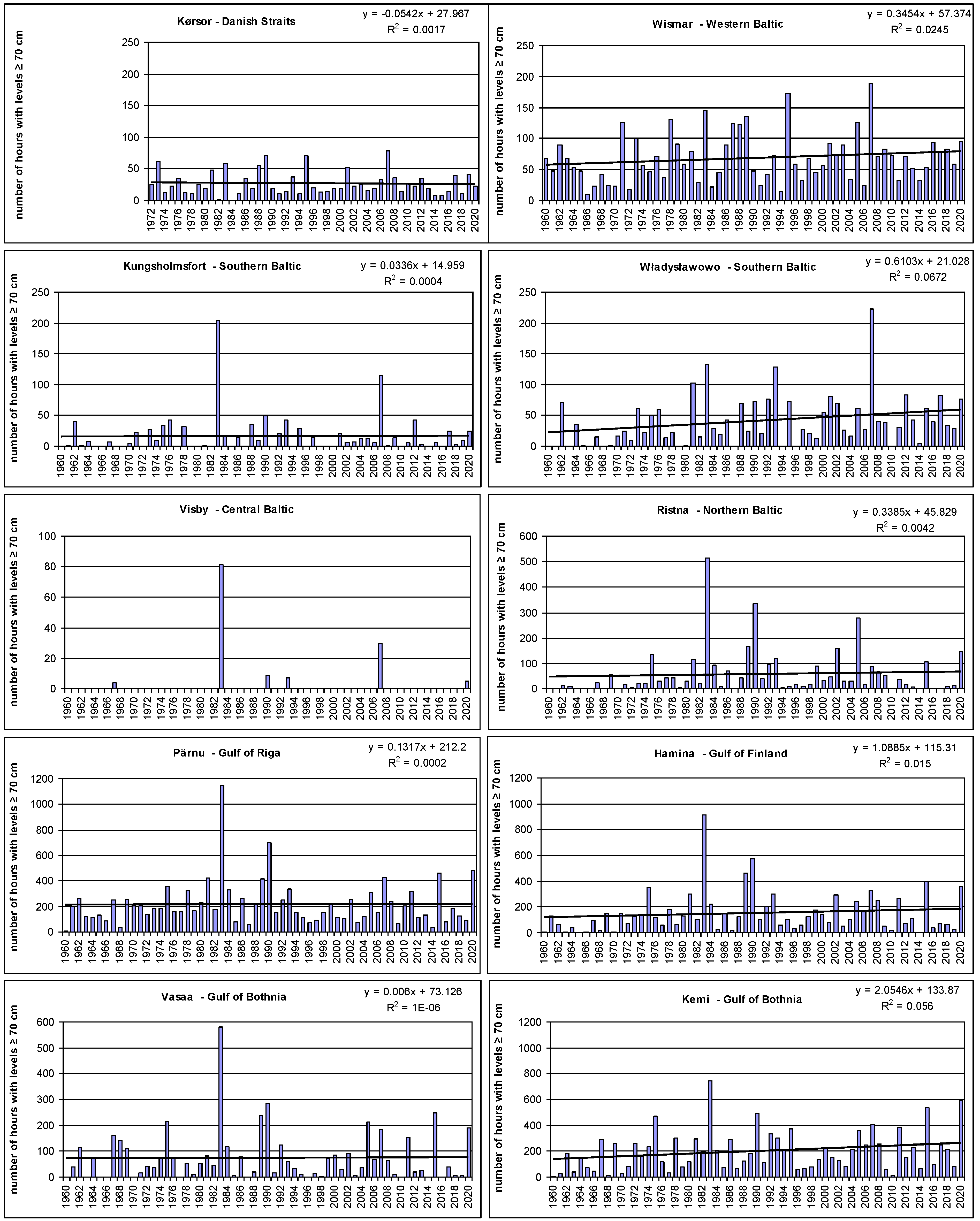
Although for most stations the trend values showed no statistical significance at α = 0.05 level, it is notable that for 8 out of 10 analyzed tide gauges, an increasing trend is observed in the duration of high sea levels from a multi-year perspective (Table 3, column 2). On average, from 1960 to 2020, the duration of high sea levels for the Baltic Sea (≥70 cm relative to tide gauge zero) increased by 1/3. The highest increases in duration of high sea levels were noted at stations situated on the open waters of the Baltic Sea, exposed to the influx of western air masses that cause a sea level rise. These are: Władysławowo (Southern Baltic, from 23 to 58 h per year) and Ristna (Northern Baltic, from 47 to 67 h per year). A second category of stations includes those situated within bays located in close proximity to the prevalent tracks of the baric depression movement: Kemi (the Gulf of Bothnia, from 136 to 259 h) and Hamina (the Gulf of Finland, from 116 to 182 h). No trend was displayed by the Visby station in the Central Baltic, located at the nodal point of the Baltic seiche, where the sea level changes display the least dynamics [12,29].
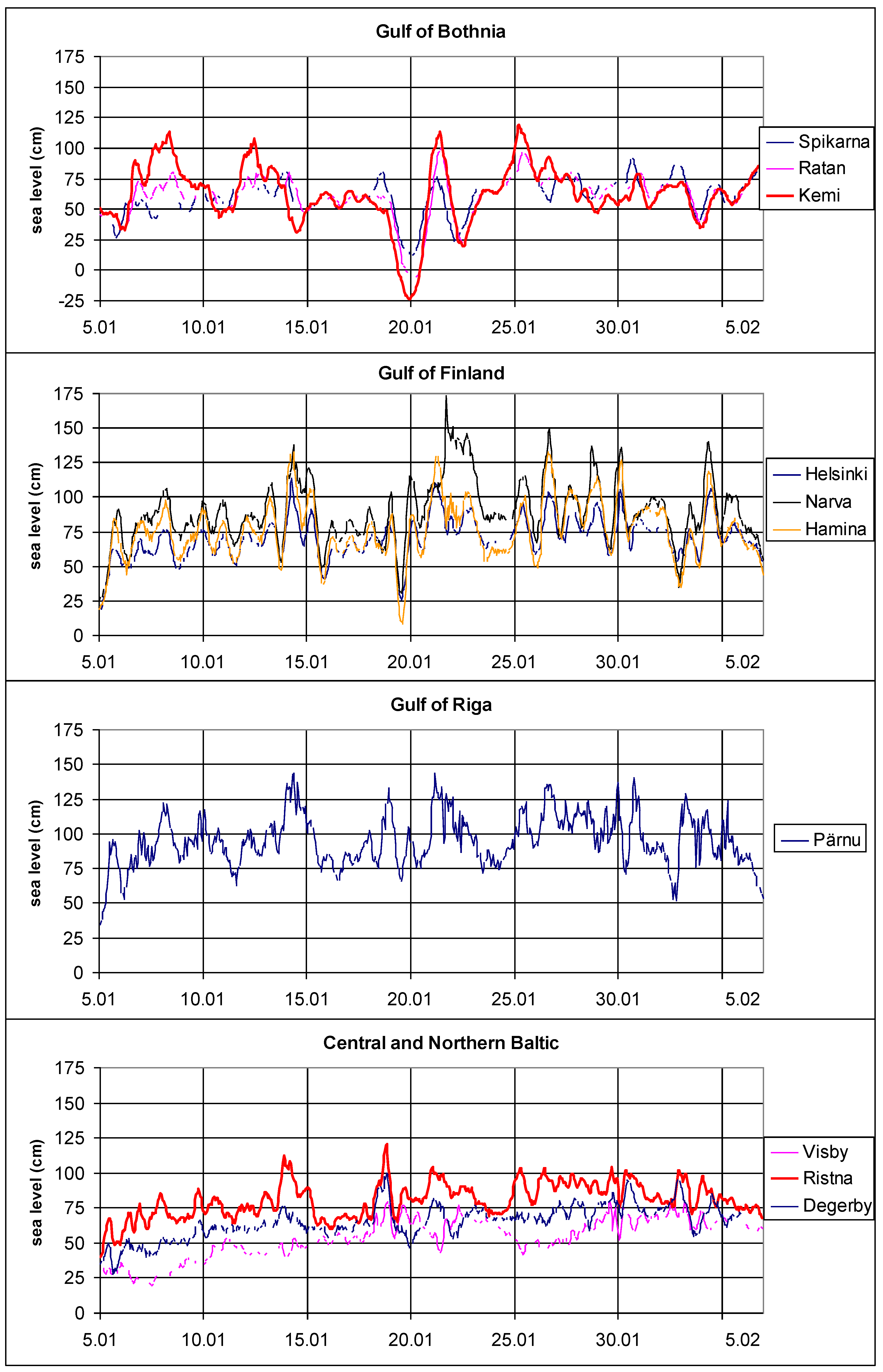
In the chart showing the duration of high sea levels (Figure 10), the year 1983 is clearly marked for the majority of the Baltic tide gauges as having the highest values from the entire length of the 1960–2020 observation series. The maximum number of hours of high water levels was due to a period of Baltic basin filling-up that lasted more than a month and took place in January and February 1983.This filling-up episode resulted from a prolonged presence of zonal western circulation over Europe. Both late 1982 and early 1983 witnessed a high number of storms, and prevalent wind directions were from the west, which sustained high water levels in the Baltic Sea [10]. Sea levels in the bays and in the Northern and Central Baltic remained within the range of high levels (from 50 to 125 cm above tide gauge zero) for nearly a month, and in the case of Narwa station (the Gulf of Finland), the maximum value for this period reached 173 cm (21 January 1983) (Figure 11).
The distribution of the number of storm surges per year in a multi-year perspective from 1960 to 2020 displays a similar trend to the changes in duration of high sea level. This is obvious, as storm surges are associated with the occurrence of high sea levels. Through the past 61 years, for most tide gauging stations at various Baltic coasts, the number of storm surges has been consistently rising (Table 3). No trend in the number of storm surges was determined only for the Visby station, located on the Swedish coast of the Central Baltic. This is due to the lack of storm surges or their single occurrences through the entire study period.
A further step in the study of extreme sea levels was the analysis of maximum annual sea levels in a multi-year perspective spanning the past 61 years. This analysis indicated a continued increase in the height of sea level maxima on the Baltic all coasts from 1960 to 2020 (Table 3). Despite the lack of statistical significance at α = 0.05 level for most tide gauges stations, such a large scale of the phenomenon lends credibility to the process of a stable increase in annual maxima. Overall, an average increase in maximum annual water levels at the Baltic Sea tide gauges equaled 0.28 cm/year. Through the whole study period, the maximum sea level has risen on average from 95 to 110 cm. The highest rate of increase was observed at the Władysławowo station (0.48 cm per year) in the Southern Baltic, and at the Ristna station (0.43 cm per year) in the Northern Baltic. Both these tide gauging stations are situated on the open waters of the Baltic Sea and thus exposed to an inflow of prevalent western air masses. At the stations located within gulfs and bays (the Gulf of Finland, the Gulf of Bothnia, the Bay of Mecklenburg), the prevalent rate of increase was higher than average, i.e., 0.28 cm per year. The lowest increasing trend was observed at the Visby station (0.02 cm per year), which is due to its central location on the Baltic Sea (i.e., nodal point of the Baltic seiche).
The above analyses indicated the existence of a clear process of increasing duration of high sea level, increase in storm surge frequency, and increase in height of maximum annual sea levels for the period 1960–2020. The main cause of these changes is the intensification of air mass inflow from the northwest in the past decades, i.e., an intensifying western circulation. The opposite advection direction, which facilitates sea level lowering, occurred significantly less frequently through this period [30]. Such interpretation is supported by numerous studies. Heyen et al. (1996) [31] observed strong relationships between pressure field anomalies over the North Atlantic and sea level anomalies for 23 tide gauging stations located along the Baltic coasts. According to Suursaar and Sooäär (2007) [32], the excessive increase in the maxima of the Estonian coastal waters (3.5–11.2 mm per year) could be explained by a local sea level response to the changing regional wind climate. All of these increases are observed for the winter half-year (from November to March), which is in agreement with similar trends in NAO and trends in storminess occurrence in this period. Johansson et al. (2001) [33] showed that sea level maxima along the Finnish coast rose significantly from 1922 to 1999. According to these authors, the elevated trends (rate 1.9–2.9 mm per year) in sea level maxima at tide gauges located in the marginal parts of the gulf and bays (Kemi and Oulu stations, the Bay of Bothnia) and Hamina (the Gulf of Finland) were due to “local storms”. Hünicke and Zorita (2006) [34], in turn, determined that the sea level increase at the Baltic Sea stations in the 1980s corresponded to the increases in average temperature, precipitation sum, and air pressure in the entire North Atlantic-European sector. According to Miętus et al. (2004) [35], the increase in intensity and stability of western air mass inflow causes the waters to be pushed through the Danish Straits and into the Baltic Sea more strongly. The opposite situation (pushing waters out of the Baltic Sea) occurs significantly less frequently. Thus, the filling of the Baltic Sea (expressed by water volume) periodically rises, and the sea level along the Polish coast is consistently rising. While considering the Baltic Sea extreme water levels, one needs to keep in mind that this basin is linked to the world ocean via the North Sea. According to the 5th IPCC report [36] and numerous studies [37,38], the increase in mean sea level (MSL) is the main (but not the only) cause for the increase in and frequency of extreme sea levels globally. The latest, 6th, IPCC report [1] assesses that between 1971 and 2006, the global mean sea level (GMSL) has been rising at a rate of 1.9 mm per year (0.8 to 2.9), and in subsequent years 2006–2018 the GMSL increase rate equaled 3.7 mm per year (3.2 to 4.2). Probably the main driver of these increases was human impact, at least since 1971. Additionally, the dominant modes of climate variability, in particular ENSO and NAO, also have a measurable impact on sea level extremes and storm activity in numerous regions [39,40,41]. A number of studies project a further increase in storm surge number and their intensity in Europe, and especially so in Great Britain and in Scandinavia [42,43]. The studies by Sztobryn et al. (2005) [10] corroborate this trend for the Southern Baltic coast. Long-term sea level records also display an increasing trend in the frequency of extreme sea level occurrences [44,45]. This trend is likely associated with the increase in cyclone activity, and westerly wind frequency over the North Atlantic and Northern Europe [46,47,48]), and over the Baltic Sea region [49,50,51]. The latest forecasts indicate that by the end of the 21st century, the frequency of strong western winds in autumn and winter will increase by as much as 50%. Concurrently, easterly winds become less common. [52] From 1948 to 2000, the number of cyclones from the North Atlantic crossing the Baltic Sea displayed an increasing trend, especially for the cool season [50]. Through the period 1948–2010, the overall number of strong cyclones (<981.1 hPa) passing over the Baltic Sea has not changed, but their average and minimum pressures have clearly decreased [53]. Between 1979 and 2015, however, the number of extreme cyclones (sometimes called ‘weather bombs’) over the North Atlantic and in the Arctic, displayed an increasing trend, rising by six events per decade [54].
4. Conclusions
The present study characterizes storm surges based on storm situations that occurred in October and November 2020 in the Baltic Sea. Based on an analysis of detailed pressure field, wind and sea level change data, two main types of storm surges were identified: the first type, with a dominant influence of the wind and the second subpressure type, with the main influence of an active and deep depression generating seiche oscillations of the water level. Given the differing coast exposure to the wind field and to the low-pressure system track, forecasting the influence of a given depression or wind field on the magnitude of a surge or water lowering may be challenging. In some cases, the wind field and subpressure cause inverse effects at a given coast section (e.g., positive phase of a low-pressure system water cushion in conjunction with a lowering effect of offshore wind). If, however, the two factors act in agreement with one another and at the same time, a large storm surge may result. Thus, it is essential for future studies on the Baltic Sea storm surge origins to incorporate the influence of both these factors in order to fully understand the peculiarities of storm surge events.
The present study also corroborated the trends in occurrences of extreme phenomena on the Baltic Sea. Through the past 60 years, the duration of high sea level on the Baltic Sea has increased by 1/3. The number of storm surges has increased on average from 3.1 to 5.5 per year. The height of maximum sea levels has also increased, with a trend value of 0.28 cm per year. These changes are caused by western circulation that has been intensifying through the late 20th and early 21st centuries and the rising global mean sea level (GMSL), both associated with global warming processes. Understanding the characteristics and trends in storm surge occurrences, presented herein, may contribute to a more accurate assessment of the influence of climate changes on threats associated with extreme sea level impact on the Baltic Sea coastal zone.
Author Contributions
Conceptualization: T.W. and B.W.; field collection: T.W.; methodology: T.W.; formal analysis: T.W. and B.W; data curation: T.W.; writing—original draft preparation: T.W.; writing—review and editing, T.W. and B.W.; visualization, T.W. All authors have read and agreed to the published version of the manuscript.
Funding
This research received no external funding.
Institutional Review Board Statement
Not applicable.
Informed Consent Statement
Not applicable.
Data Availability Statement
1. Hourly sea levels data are available in the national hydrological and meteorological institutes of the Baltic states: SMHI (Sweden, https://www.smhi.se/en/services/open-data/national-archive-for-oceanographic-data, accessed on 1 October 2021), FMI (Finland, https://www.ilmatieteenlaitos.fi/havaintojen-lataus, accessed on 1 October 2021), DMI (Denmark, https://www.dmi.dk/index.php?id=1231&L=0, accessed on 1 October 2021), BSH (Germany, https://www.pegelonline.wsv.de/, accessed on 1 October 2021), EMHI (Estonia), LEGMC (Latvia), EPA (Lithuania), IMGW (Poland, https://danepubliczne.imgw.pl/datastore, accessed on 1 October 2021). 2. Hourly wind data are available at: National Centers for Environmental Information, Climate Data Online, https://www.ncdc.noaa.gov/cdo-web/, accessed on 1 October 2021. 3. Synoptic maps are available from the Met Office, https://digital.nmla.metoffice.gov.uk/SO_4d70038f-c03f-4cb2-818e-7bc3aec7cfb0/, accessed on 1 October 2021.
Acknowledgments
We wish to thank the national hydrological and meteorological institutes of the states of the Baltic Sea—SMHI (Sweden), FMI (Finland), DMI (Denmark), BSH (Germany), EMHI (Estonia), LEGMC (Latvia), EPA (Lithuania), IMGW (Poland)—for providing the sea level data.
Conflicts of Interest
The authors declare no conflict of interest.
References
- IPCC. Sea Level. In Sixth Assessment Report AR6, Climate Change 2021: The Physical Science Basis, 1st ed.; Masson-Delmotte, V.P., Zhai, A., Eds.; Cambridge University Press: Cambridge, UK, 2021; pp. 44–46. [Google Scholar]
- Kowalewska-Kalkowska, H. Rola Wezbrań Sztormowych w Kształtowaniu Ustroju Wodnego Układu Dolnej Odry i Zalewu Szczecińskiego, Impacts of Storm Surgeson the Water Lewel in the System of Downstream Reaches of the Odra River and the Szczecin lagoon, 1st ed.; Wydawnictwo Naukowe Uniwersytetu Szczecińskiego: Szczecin, Poland, 2012; pp. 1–258. (In Polish) [Google Scholar]
- Wiśniewski, B.; Wolski, T. Physical aspects of extreme storm surges and falls on the Polish coast. Oceanologia 2011, 53, 373–390. [Google Scholar] [CrossRef] [Green Version]
- Gustafsson, B.; Andersson, H. Modeling the exchange of the Baltic Sea from the meridional atmospheric pressure difference across the North Sea. J. Geophys. Res. 2001, 106, 19731–19744. [Google Scholar] [CrossRef]
- Averkiev, A.S.; Klevanny, K.A. Case study of the impact of cyclonic trajectories on sea-level extremes in the Gulf of Finland. Cont. Shelf Res. 2010, 30, 707–714. [Google Scholar] [CrossRef]
- Suursaar, Ü. Wind and wave storms, storm surges and sea level rise along the Estonian coast of the Baltic Sea. Oceanologia 2010, 52, 391–416. [Google Scholar] [CrossRef] [Green Version]
- Suursaar, Ü.; Kullas, T.; Otsmann, M.; Kõuts, T. Extreme sea level events in the coastal waters of western Estonia. J. Sea Res. 2003, 49, 295–303. [Google Scholar] [CrossRef] [Green Version]
- Suursaar, Ü.; Kullas, T.; Szava-Kovats, R. Wind and wave storms, storm surges and sea level rise along the Estonian coast of the Baltic Sea. In Management of Natural Resources, Sustainable Development and Ecological Hazards II, 1st ed.; WIT Transactions on Ecology and the Environment: Southampton, UK, 2009; Volume 127, pp. 149–160. [Google Scholar] [CrossRef] [Green Version]
- Rosenhagen, G.; Bork, I. Rekonstruktion der Sturmflutwetterlage vom 13. November 1872. Die Küste 2009, 75, 51–70. (In German) [Google Scholar]
- Sztobryn, M.; Stigge, H.J.; Wielbińska, D.; Weidig, B.; Stanisławczyk, I.; Kańska, A.; Mykita, M. Storm Surges in the Southern Baltic (Western and Central Parts), 1st ed.; Bundesamtes für Seeschifffahrt und Hydrographie: Rostock, Germany, 2005; Volume 39, pp. 1–74.
- Wolski, T.; Wiśniewski, B.; Musielak, S. Baltic Sea datums and their unification as a basis for coastal zone and seabed studies. Oceanol. Hydrobiol. Stud. 2016, 45, 239–258. [Google Scholar] [CrossRef]
- Wolski, T.; Wiśniewski, B. Geographical diversity in the occurrence of extreme sea levels on the coasts of the Baltic Sea. J. Sea Res. 2020, 159, 101890. [Google Scholar] [CrossRef]
- Wolski, T.; Wiśniewski, B. The Probability of occurrence of extreme sea levels on coasts of the Baltic Sea. J. Coast. Res. 2020, 95, 1349–1354. [Google Scholar] [CrossRef]
- Sahebjalal, E. Application of Geostatistical Analysis for Evaluating Variation in Groundwater Characteristics. World Appl. Sci. J. 2012, 18, 135–141. [Google Scholar]
- Badura, H.; Zawadzki, J.; Fabijańczyk, P. Block kriging and gis methods in geostatistical modeling of methane gas content in coal mines. Rocz. Geomatyki 2012, 10, 17–26, (In Polish, Abstract in English). [Google Scholar]
- SMHI. Swedish Meteorological and Hydrological Institute. Varningsdefinitioner. Available online: https://edmo.seadatanet.org/report/545 (accessed on 6 October 2021).
- FMI. Finnish Meteorological Institute. Meriveden Korkeusvaroitus. Available online: http://ilmatieteenlaitos.fi/tietoa-merivedenkorkeusvaroitus (accessed on 6 October 2021).
- IMGW. Institute of Meteorology and Water Management-National Research Institute. Available online: http://monitor.pogodynka.pl/#map/18.3314,53.5011,8,true,true,0 (accessed on 6 October 2021).
- Hupfer, P.; Harff, J.; Sterr, H.; Stigge, H.J. Die Wasserstände an der Ostseeküste. Entwicklung–Sturmfluten–Klimawandel 3, Hoch- und Niedrigwasser. Die Küste 2003, 66, 106–216. (In German) [Google Scholar]
- Tiesel, R. Weather of the Baltic Sea. In State and Evolution of the Baltic Sea, 1952–2005: A Detailed 50-Year Survey of Meteorology and Climate, Physics, Chemistry, Biology and Marine Environment, 1st ed.; Feistel, R., Nausch, G., Wasmund, N., Eds.; John Wiley & Sons: New York, NY, USA, 2008; pp. 65–92. [Google Scholar]
- Jensen, J.; Müller-Navara, S.H. Storm surges on the German Coast. Die Küste 2008, 74, 92–124. [Google Scholar]
- Sztobryn, M.; Weidig, B.; Stanisławczyk, I.; Holfort, J.; Kowalska, B.; Mykita, M.; Kańska, A.; Krzysztofik, K.; Perlet, I. Negative Surges in the Southern Baltic Sea (Western and Central Parts), 1st ed.; Bundesamtes für Seeschifffahrt und Hydrographie: Hamburg, Germany, 2009; pp. 1–71.
- Averkiev, A.S.; Klevanny, K.A. Determining cyclone trajectories and velocities leading to extreme sea level rises in the Gulf of Finland. Russ. Meteorol. Hydrol. 2007, 32, 514–519. [Google Scholar] [CrossRef]
- Jaagus, J.; Suursaar, Ü. Long-term storminess and sea level variations on the Estonian coast of the Baltic Sea in relation to large-scale atmospheric circulation, Estonian. J. Earth Sci. 2013, 62, 73–92. [Google Scholar] [CrossRef]
- Lisowski, K. Nieokresowe wahania poziomu Bałtyku pod wpływem czynników anemobarycznych [Non-periodic fluctuations in the level of the Baltic Sea under the influence of anemobaric factors]. Arch. Hydrotech. 1961, 8, 17–42. (In Polish) [Google Scholar]
- Wolski, T.; Wiśniewski, B.; Giza, A.; Kowalewska-Kalkowska, H.; Boman, H.; Grabbi-Kaiv, S.; Hammarklint, T.; Holfort, J.; Lydeikaite, Z. Extreme sea levels at selected stations on the Baltic Sea coast. Oceanologia 2014, 56, 259–290. [Google Scholar] [CrossRef] [Green Version]
- Doodson, A.T.; Warburg, H.D. Admiralty Manual of Tides, 1st ed.; Her Majesty’s Stationery Office: London, UK, 1941; pp. 1–270.
- Pugh, D.T. Tides, Surges and Mean Sea-Level, 1st ed.; John Wiley & Sons: New York, NY, USA, 1987; pp. 1–472. [Google Scholar]
- Leppäranta, M.; Myrberg, K. Physical Oceanography of the Baltic Sea, 1st ed.; Springer Science & Business Media: Berlin, Germany, 2009; pp. 1–378. [Google Scholar]
- Moberg, A.; Tuomenvirta, H.; Nordli, P.Ø. Recent climatic trends. In The Physical Geography of Fennoscandia, 1st ed.; Seppälä, M., Ed.; Oxford University Press: Oxford, UK, 2005; pp. 113–133. [Google Scholar]
- Heyen, H.; Zorita, E.; von Storch, H. Statistical downscaling of monthly mean North Atlantic air-pressure to sea-level anomalies in the Baltic Sea. Tellus 1996, 48, 312–323. [Google Scholar] [CrossRef] [Green Version]
- Suursaar, Ü.; Sooäär, J. Decadal variations in mean and extreme sea level values along the Estonian coast of the Baltic Sea. Tellus 2007, 59, 249–260. [Google Scholar] [CrossRef]
- Johansson, M.; Boman, H.; Kahma, K.; Launiainen, J. Trends in sea level variability in the Baltic Sea. Boreal Environ. Res. 2001, 6, 159–179. [Google Scholar]
- Hünicke, B.; Zorita, E. Influence of temperature and precipitation on decadal Baltic Sea level variations in the 20th century. Tellus 2006, 58, 141–153. [Google Scholar] [CrossRef] [Green Version]
- Miętus, M.; Filipiak, J.; Owczarek, M. Klimat wybrzeża południowego Bałtyku. Stan obecny i perspektywy zmian [The Climate of the Southern Baltic Coast. Current State and Prospects for Changes]. In Środowisko Polskiej Strefy Południowego Bałtyku–Stan Obecny i Przewidywanie Zmiany w Przededniu Integracji Europejskiej, 1st ed.; Cyberski, J., Ed.; GTN: Gdańsk, Poland, 2004; pp. 11–44. [Google Scholar]
- IPCC. Sea Level Change. In Fifth Assessment Report of the IPCC, Climate Change 2013 The Physical Science Basis; Stocker, T.F., Qin, D., Eds.; Cambridge University Press: Cambridge, UK, 2013; pp. 1137–1216. [Google Scholar]
- Menéndez, M.; Woodworth, P.L. Changes in extreme high water levels based on a quasi-global tidegauge data set. J. Geophys. Res. Ocean 2010, 115, 1–15. [Google Scholar] [CrossRef] [Green Version]
- Pugh, D.T.; Woodworth, P. Sea-Level Science. Understanding Tides, Surges, Tsunamis and Mean Sea-Level Changes, 1st ed.; Cambridge University Press: Cambridge, UK, 2014; pp. 1–407. [Google Scholar]
- Lowe, J.A.; Woodworth, P.L.; Knutson, T.; McDonald, R.E.; McInnes, K.L.; Woth, K.; von Storch, H.; Wolf, J.; Swail, V.; Bernier, N.B.; et al. Past and future changes in extreme sea levels and waves. In Understanding Sea-Level Rise and Variability, 1st ed.; Church, J.A., Woodworth, P.L., Aadrup, T., Wilson, W.S., Eds.; Wiley-Blackwell: Hoboken, NJ, USA, 2010; pp. 326–375. [Google Scholar]
- Walsh, K.J.; McInnes, E.K.; McBride, J.L. Climate change impacts on tropical cyclones and extremesea levels in the South Pacific–a regional assessment. Glob. Planet. Chang. 2011, 80–81, 149–164. [Google Scholar]
- Vermaire, J.C.; Pisaric, M.F.J.; Thienpont, J.R.; Mustaphi, C.J.C.; Kokelj, S.V.; Smol, J.P. Arctic climate warming and sea ice declines lead to increased storm surge activity. Geophys. Res. Lett. 2013, 40, 1386–1390. [Google Scholar] [CrossRef]
- Bengtsson, L.; Hodges, K.; Roeckner, E. Storm tracks and climate change. J. Clim. 2006, 19, 3518–3543. [Google Scholar] [CrossRef] [Green Version]
- Fischer-Bruns, I.; Von Storch, H.; Gonzalez-Rouco, J.F.; Zorita, E. Modelling the variability of midlatitude storm activity on decadal to century time scales. Clim. Dyn. 2005, 25, 461–476. [Google Scholar] [CrossRef]
- Bouligand, R.; Pirazzoli, P.A. Positive and negative sea surges at Brest. Oceanol. Acta 1999, 22, 153–166. [Google Scholar] [CrossRef] [Green Version]
- Woodworth, P.L.; Blackman, D.L. Changes in extreme high waters at Liverpool since 1768. Int. J. Climatol. 2002, 22, 697–714. [Google Scholar] [CrossRef]
- McCabe, G.J.; Clark, M.P.; Serreze, M.C. Trends in Northern Hemisphere surface cyclone frequency and intensity. J. Clim. 2001, 14, 2763–2768. [Google Scholar] [CrossRef]
- Zhang, X.; Walsh, J.E.; Zhang, J.; Bhatt, U.S.; Ikeda, M. Climatology and interannual variability of Arctic cyclone activity: 1948–2002. J. Clim. 2004, 17, 2300–2317. [Google Scholar] [CrossRef]
- Pinto, J.G.; Ulbrich, U.; Leckebusch, G.C.; Spangehl, T.; Reyers, M.; Zacharias, S. Changes in storm track and cyclone activity in three SRES ensemble experiments with the ECHAM5/MPI-OM1 GCM. Clim. Dyn. 2007, 29, 195–210. [Google Scholar] [CrossRef]
- Link, P.; Post, P. Spatial and temporal variance of cyclones in the Baltic Sea region. In Session AW8: Weather Types classifications, Proceedings of the 5th Annual Meeting of the European Meteorological Society, Utrecht, The Netherlands, 12–16 September 2005; COST Action 733; EU Publications Office: Luxembourg, 2007; pp. 69–76. [Google Scholar]
- Sepp, M.; Post, P.; Jaagus, J. Long-term changes in the frequency of cyclones and their trajectories in Central and Northern Europe. Nord. Hydrol. 2005, 36, 297–309. [Google Scholar] [CrossRef]
- Sepp, M. Changes in frequency of Baltic Sea cyclones and their relationships with NAO and climate in Estonia. Boreal Environ. Res. 2009, 14, 143–151. [Google Scholar]
- Ruosteenoja, K.; Vihma, T.; Venäläinen, A. Projected changes in European and North Atlantic seasonal wind climate derived from CMIP5 simulations. J. Clim. 2019, 32, 6467–6490. [Google Scholar] [CrossRef]
- Sepp, M.; Mändla, K.; Post, P. On the Origins of Cyclones Entering the Baltic Sea Region, In EMS Annual Meeting Abstracts; European Meteorological Society: Berlin, Germany, 2014; Volume 11. [Google Scholar]
- Rinke, A.; Maturilli, M.; Graham, R.M.; Matthes, H.; Handorf, D.; Cohen, L.; Moore, J.C. Extreme cyclone events in the Arctic: Wintertime variability and trends. Environ. Res. Lett. 2017, 12, 094006. [Google Scholar] [CrossRef]
Figure 1.
Division of the Baltic Sea into primary sub-basins.

Figure 2.
The course of the low pressure system between 13 and 15 October 2020, along with the main synoptic situation on 14 October 2020, 18:00 h UTC (source: Met Office, modified, © British Crown copyright, Met Office).
Figure 2.
The course of the low pressure system between 13 and 15 October 2020, along with the main synoptic situation on 14 October 2020, 18:00 h UTC (source: Met Office, modified, © British Crown copyright, Met Office).

Figure 3.
Sea level changes for representative stations in the main sub-basins of the Baltic Sea from 13 to 16 October 2020. (Storm surge at the Wismar station in the Western Baltic, and low sea levels at the northeastern Baltic coasts).
Figure 3.
Sea level changes for representative stations in the main sub-basins of the Baltic Sea from 13 to 16 October 2020. (Storm surge at the Wismar station in the Western Baltic, and low sea levels at the northeastern Baltic coasts).

Figure 4.
Distribution of wind direction and velocity together with sea level changes in individual Baltic Sea sub-basins from 13 to 16 October 2020. A stable increase followed by slow decrease in sea level in the Western Baltic (the stations at Skanör, Wismar, and Świnoujście) driven by changes in velocity of the northeastern onshore wind. (Legends: blue line—sea level; black arrow—wind direction; columns—wind velocity).

Figure 5.
Instantaneous sea levels on the Baltic Sea from 13 to 16 October 2020. (Storm surge rising and falling in the Western Baltic due to wind impact).
Figure 5.
Instantaneous sea levels on the Baltic Sea from 13 to 16 October 2020. (Storm surge rising and falling in the Western Baltic due to wind impact).

Figure 6.
The course of the low pressure system on 20–24 November 2020 together with the main synoptic situation on 21 November 2020, 18:00 h UTC (source: Met Office, modified, © British Crown copyright, Met Office).
Figure 6.
The course of the low pressure system on 20–24 November 2020 together with the main synoptic situation on 21 November 2020, 18:00 h UTC (source: Met Office, modified, © British Crown copyright, Met Office).

Figure 7.
Sea level changes at representative stations in the main basins of the Baltic Sea from 20 to 23 November 2020. (Alternating, seiche-like sea level oscillations between the southwestern and northeastern Baltic coasts).
Figure 7.
Sea level changes at representative stations in the main basins of the Baltic Sea from 20 to 23 November 2020. (Alternating, seiche-like sea level oscillations between the southwestern and northeastern Baltic coasts).

Figure 8.
Wind direction and velocity distribution, along with sea level changes in individual sub-basins of the Baltic Sea from 20 to 23 November 2020. The influence of subpressure associated with an active low-pressure area. A dynamic sea level rise in the Western Baltic (at Wismar, Skänor, and Świnoujście stations) despite an offshore wind. A sea level decrease and increase during a period of stable onshore winds from the southwest at the stations at Pärnu (the Gulf of Riga) and Hamina (the Gulf of Finland). (Legends: blue line—sea level, black arrow—wind direction, columns—wind velocity).

Figure 9.
Instantaneous sea levels on the Baltic Sea from 20 to 23 November 2020. (A characteristic phenomenon of alternating sea level oscillations between southwestern and northeastern sub-basins of the Baltic Sea).
Figure 9.
Instantaneous sea levels on the Baltic Sea from 20 to 23 November 2020. (A characteristic phenomenon of alternating sea level oscillations between southwestern and northeastern sub-basins of the Baltic Sea).

Figure 10.
Duration of high sea levels (≥70 cm relative to zero of tide gauge) at selected tide gauges and their trends through the study period 1960–2020. The year 1982 stands out as the period characterized by the longest duration (i.e., the highest number of hours) of high sea levels in a multi-year perspective. (Legends: blue columns —number of hours of high sea levels).

Figure 11.
Example of filling the Baltic Sea sub-basins between 5 January and 5 February 1983. Sustained high sea levels result from prolonged western circulation and a significant influx of waters from the North Sea.
Figure 11.
Example of filling the Baltic Sea sub-basins between 5 January and 5 February 1983. Sustained high sea levels result from prolonged western circulation and a significant influx of waters from the North Sea.


Table 1.
Features of the low pressure system and parameters of the storm surge analyzed in the period of 13–16 October 2020.
Table 1.
Features of the low pressure system and parameters of the storm surge analyzed in the period of 13–16 October 2020.
| Tide Gauge | Features of the Low Pressure System | Recorded Sea Level | ||||||||||
|---|---|---|---|---|---|---|---|---|---|---|---|---|
| pi (hPa) | VL (m/s) | Initial Sea Level (cm) | Max. (cm) | Min. (cm) | Amplitude (cm) | The Maximum Rate of Sea Level Change (cm/h) | Duration of Sea Level (h) | |||||
| Rise | Fall | ≥ | ≤ | |||||||||
| 70 cm | 100 cm | −70 cm | −100 cm | |||||||||
| Kørsor | 1004 | 7.77 | −6 | 69 | −16 | 85 | 11 | 9 | ||||
| Wismar | 16 | 140 | 0 | 140 | 13 | 11 | 30 | 18 | ||||
| Skanör | 1 | 84 | −2 | 86 | 8 | 9 | 5 | |||||
| Świnoujście | 8 | 110 | 8 | 102 | 12 | 9 | 30 | 10 | ||||
| Kungsholmsfort | 3 | 47 | −5 | 52 | 5 | 4 | ||||||
| Visby | 2 | 7 | −14 | 21 | 2 | 3 | ||||||
| Ristna | 2 | 2 | −42 | 44 | 2 | 3 | ||||||
| Pärnu | 12 | 13 | −77 | 90 | 8 | 8 | 9 | |||||
| Hamina | 6 | 6 | −50 | 56 | 5 | 5 | ||||||
| Kemi | −6 | −6 | −52 | 46 | 3 | 4 | ||||||
Table 2.
Features of the low pressure system and parameters of the storm surge analyzed in the period of 20–23 November 2020.
Table 2.
Features of the low pressure system and parameters of the storm surge analyzed in the period of 20–23 November 2020.
| Tide Gauge | Features of the Low Pressure System | Recorded Sea Level | ||||||||||
|---|---|---|---|---|---|---|---|---|---|---|---|---|
| pi (hPa) | VL (m/s) | Initial Sea Level (cm) | Max. (cm) | Min. (cm) | Amplitude (cm) | The Maximum Rate of Sea Level Change (cm/h) | Duration of Sea Level (h) | |||||
| Rise | Fall | ≥ | ≤ | |||||||||
| 70 cm | 100 cm | −70 cm | −100 cm | |||||||||
| Kørsor | 963 | 17.5 | 25 | 67 | −35 | 108 | 13 | 15 | 2 | |||
| Wismar | −46 | 65 | −96 | 161 | 22 | 11 | 12 | |||||
| Skanör | 25 | 35 | −100 | 135 | 23 | 19 | 7 | |||||
| Świnoujście | 17 | 41 | −77 | 118 | 16 | 15 | 4 | |||||
| Kungsholmsfort | 17 | 34 | −51 | 85 | 11 | 9 | ||||||
| Visby | 15 | 31 | 6 | 25 | 6 | 6 | ||||||
| Ristna | 16 | 109 | 16 | 93 | 26 | 19 | 9 | 7 | ||||
| Pärnu | 78 | 129 | 30 | 99 | 15 | 29 | 26 | 8 | ||||
| Hamina | 50 | 121 | 11 | 110 | 16 | 16 | 20 | 6 | ||||
| Kemi | 30 | 92 | −26 | 118 | 12 | 11 | 28 | |||||
Table 3.
Trends in duration of high sea levels ≥ 70 cm per year and in the number of storm surges per year, along with trends in the maximum annual sea level values determined from the trend line for the Baltic Sea tide gauging stations at the beginning and at the end of the 1960–2020 period *.
Table 3.
Trends in duration of high sea levels ≥ 70 cm per year and in the number of storm surges per year, along with trends in the maximum annual sea level values determined from the trend line for the Baltic Sea tide gauging stations at the beginning and at the end of the 1960–2020 period *.
| Station | Trend in Duration of High Sea Levels ≥ 70 cm (hours) | Trends in Number of Storm Surges | Trend in the Height of Maximum Annual Sea Levels | |
|---|---|---|---|---|
| (cm/year) | (cm) | |||
| Kørsor—Danish Straits | 28 → 25 | 3.3 → 3.7 | 0.23 | 93 → 103 |
| Wismar—Western Baltic | 58 → 78 | 4.0→ 7.1 | 0.36 | 115→ 136 |
| Kungsholmsfort—Southern Baltic | 15 → 17 | 1.2 → 1.4 | 0.17 | 74 → 84 |
| Władysławowo—Southern Baltic | 23→ 58 | 1.7 → 3.3 | 0.48 | 79→ 107 |
| Visby—Central Baltic | 2 → 2 | - | 0.02 | 54 → 55 |
| Ristna—Northern Baltic | 47 → 67 | 2.5 → 3.6 | 0.43 | 88 → 113 |
| Pärnu—Gulf of Riga | 212 → 220 | 7.3 → 11.2 | 0.13 | 139 → 147 |
| Hamina—Gulf of Finland | 116 → 182 | 5.5→ 11.5 | 0.33 | 110 → 130 |
| Vasaa—Gulf of Bothnia | 73 → 74 | 1.0→ 2.9 | 0.32 | 78→ 97 |
| Kemi—Gulf of Bothnia | 136→ 259 | 4.8→ 9.7 | 0.29 | 119 → 134 |
| Total Baltic Sea | 71 → 98 | 3.1 → 5.5 | 0.28 | 95 → 111 |
* The station at Kørsor—in the Danish Straits was characterized by a shorter study period, spanning 1972–2020.
Publisher’s Note: MDPI stays neutral with regard to jurisdictional claims in published maps and institutional affiliations. |
© 2021 by the authors. Licensee MDPI, Basel, Switzerland. This article is an open access article distributed under the terms and conditions of the Creative Commons Attribution (CC BY) license (https://creativecommons.org/licenses/by/4.0/).
Share and Cite
MDPI and ACS Style
Wolski, T.; Wiśniewski, B. Characteristics and Long-Term Variability of Occurrences of Storm Surges in the Baltic Sea. Atmosphere 2021, 12, 1679. https://0-doi-org.brum.beds.ac.uk/10.3390/atmos12121679
AMA Style
Wolski T, Wiśniewski B. Characteristics and Long-Term Variability of Occurrences of Storm Surges in the Baltic Sea. Atmosphere. 2021; 12(12):1679. https://0-doi-org.brum.beds.ac.uk/10.3390/atmos12121679
Chicago/Turabian StyleWolski, Tomasz, and Bernard Wiśniewski. 2021. "Characteristics and Long-Term Variability of Occurrences of Storm Surges in the Baltic Sea" Atmosphere 12, no. 12: 1679. https://0-doi-org.brum.beds.ac.uk/10.3390/atmos12121679
Note that from the first issue of 2016, this journal uses article numbers instead of page numbers. See further details here.