Reconstruction of the Interannual to Millennial Scale Patterns of the Global Surface Temperature


Department of Earth Sciences, Environment and Georesources, University of Naples Federico II, Complesso Universitario di Monte S. Angelo, Via Cinthia, 21, 80126 Naples, Italy
Atmosphere 2021, 12(2), 147; https://0-doi-org.brum.beds.ac.uk/10.3390/atmos12020147
Submission received: 31 December 2020
/
Revised: 14 January 2021
/
Accepted: 19 January 2021
/
Published: 24 January 2021
(This article belongs to the Section Climatology)
Abstract
:Climate changes are due to anthropogenic factors, volcano eruptions and the natural variability of the Earth’s system. Herein the natural variability of the global surface temperature is modeled using a set of harmonics spanning from the inter-annual to the millennial scales. The model is supported by the following considerations: (1) power spectrum evaluations show 11 spectral peaks (from the sub-decadal to the multi-decadal scales) above the 99% confidence level of the known temperature uncertainty; (2) spectral coherence analysis between the independent global surface temperature periods 1861–1937 and 1937–2013 highlights at least eight common frequencies between 2- and 20-year periods; (3) paleoclimatic temperature reconstructions during the Holocene present secular to millennial oscillations. The millennial oscillation was responsible for the cooling observed from the Medieval Warm Period (900–1400) to the Little Ice Age (1400–1800) and, on average, could have caused about 50% of the warming observed since 1850. The finding implies an equilibrium climate sensitivity of 1.0–2.3 °C for CO doubling likely centered around 1.5 °C. This low sensitivity to radiative forcing agrees with the conclusions of recent studies. Semi-empirical models since 1000 A.D. are developed using 13 identified harmonics (representing the natural variability of the climate system) and a climatic function derived from the Coupled Model Intercomparison Project 5 (CMIP5) model ensemble mean simulation (representing the mean greenhouse gas—GHG, aerosol, and volcano temperature contributions) scaled under the assumption of an equilibrium climate sensitivity of 1.5 °C. The harmonic model is evaluated using temperature data from 1850 to 2013 to test its ability to predict the major temperature patterns observed in the record from 2014 to 2020. In the short, medium, and long time scales the semi-empirical models predict: (1) temperature maxima in 2015–2016 and 2020, which is confirmed by the 2014–2020 global temperature record; (2) a relatively steady global temperature from 2000 to 2030–2040; (3) a 2000–2100 mean projected global warming of about 1 °C. The semi-empirical model reconstructs accurately the historical surface temperature record since 1850 and hindcasts mean surface temperature proxy reconstructions since the medieval period better than the model simulation that is unable to simulate the Medieval Warm Period.
1. Introduction
Numerous studies highlighted that the climate system is modulated by oscillations likely induced by a number of astronomical phenomena [1]. These oscillations nearly cover the entire spectrum: the daily (0–25 h), the monthly (25 h–0.5 year), the annual (0.5–2.5 year), the interannual, (2.5–10 year), the decadal/secular (10–400 year), the millennial (400–10,000 year) and Milankovitch (10,000–1,000,000 year) scales. Longer oscillations are also observed at the tectonic (1–600 million year) scales. These spectral bands are characterized by soli-lunar tidal oscillations, solar oscillations, terrestrial orbital oscillations, and galactic oscillations linked to the journey of the solar system around the galaxy [2,3,4,5,6,7,8,9,10]. Multiple criteria suggest that solar and astronomical quasi-harmonic forcing modulate a number of terrestrial variables: C and Be production, Earth’s rotation, ocean circulation, paleoclimate, geomagnetism, etc. [11,12]. These results suggest that harmonic models could approximately capture part of the natural variability of the climate under the condition that the frequencies chosen to represent it have a physical origin. In this regards, it is worth noting that the most accurate and well known geophysical model is the tidal one, where up to 40 harmonics are used to forecast tidal levels at multiple time scales [13].
In contrast, it is observed an absence of internal multidecadal and interdecadal oscillations in climate model simulations [5,14,15], which likely indicates that the physical origin of most of the observed climatic patterns is still unknown. Yet, if the claimed climatic oscillations are real [16], they cannot be ignored for correctly interpreting climate changes. For example, several studies showed that the Holocene has been characterized by a very large quasi-millennial oscillation [4,17,18,19,20,21,22,23,24]. This large oscillation was responsible for several warm periods such as those that occurred during the Roman and Medieval times [17,21,25]. The existence of such a millennial oscillation would have important implications for the correct interpretation of the observed post-industrial global warming [5].
The frequency range from the interannual to the millennial scales during the last century and millennia are particularly important to properly understanding and modeling the natural climatic variability necessary for validating the climate models and for providing reliable climate projections and forecasts for the near future. In the scientific literature, many relevant climatic oscillations have been hypothesized such as the Atlantic Multidecadal Oscillation, the El Niño Southern Oscillation, the Pacific decadal oscillations, the Interdecadal Pacific Oscillation, the Arctic Oscillation, the North Atlantic Oscillation, the North Pacific Oscillation, and others [26].
The Intergovernmental Panel on Climate Change Fifth Assessment Report [27] acknowledges that the natural climatic variability of the climate system is still not understood well and that the Coupled Model Intercomparison Project 5 (CMIP5) global circulation models (GCMs) poorly simulate it. In fact, a mismatch has been observed between the model predictions and the data, such as the temperature standstill observed since 2000 that has been not reproduced by the models predicting warming of about 2 °C/century: see Figure 1 [5,28,29].
A significant mismatch between climate model predictions and data has also been observed throughout the Holocene (during the last 10,000 year) where climate models simulate continuous global warming, mainly in response to rising CO and the retreat of ice sheets, while marine and terrestrial proxy records suggest global cooling during the Late Holocene, following the peak warming of the Holocene Thermal Maximum (from about 10,000 to 6000 year ago) [30,31]. Indeed, according to Milanković theory, the Earth’s climate should be approaching the next ice age due to astronomical orbital oscillations [32] although the exact involved physical mechanisms are still unknown. Understanding the climatic changes of the past—e.g., why the last interglacial warm period (130,000–116,000 years before present) was warmer than the Holocene—is still challenging, but improvements are made [33].
Current climate models use radiative forcing (RF) functions as their external inputs [27]. These functions include a total solar irradiance forcing, a volcano forcing, and several anthropogenic forcing functions deduced from atmospheric concentration variations of greenhouse gases (GHG), aerosol, land-use change, and others ([27], Figure 8.18). The models process them to obtain climatic functions such as local and global surface temperatures. At equilibrium, the global mean surface temperature response to a radiative forcing variation is determined by the equation , where is the equilibrium climate sensitivity (ECS) to radiative forcing. Doubling the CO atmospheric concentration results in an additional forcing of W/m that should induce about 1 °C warming [34]. In fact, according to the Stefan–Boltzmann law (), to increase by 1 °C the temperature of a black-body at a temperature K (which would be the mean Earth’s temperature if our planet was a black-body without feedbacks) a radiation increase of W/mK would be needed.
The value of is very uncertain because the physics of the main climatic feedbacks (water vapor and cloud cover) is still poorly understood [35,36]. However, the IPCC AR5 [27] reports that the net feedback should be positive and that the climate sensitivity likely range should be between 1.5 and 4.5 °C for CO doubling. In general, it is claimed to be unlikely that the ECS is less than 1 °C or larger than 6 °C [36]. The IPCC ([27], page 745) states the “very high confidence that the primary factor contributing to the spread in equilibrium climate sensitivity continues to be the cloud feedback”.
The ECS of the CMIP5 models ranges from 2.1 to 4.7 °C, with an average of about 3 °C for CO doubling, and is very similar to the assessment found in the IPCC AR4 (2007) where the CMIP3 models were used ([27], p. 745). Because the climate sensitivity to radiative forcing is not known with sufficient accuracy, if, for example, the real were close to 1.5 °C then the CMIP5 models would have on average overestimated the RF warming by a factor of 2; if, on the contrary, were close to 4.5 °C then the CMIP5 models would have on average underestimated the RF warming by 50%. Reducing this large uncertainty is necessary for understanding climatic changes [35,36].
It has been shown that the CMIP5 models are on average able to approximately reproduce the 0.85 °C warming observed from 1860 to 2000: Figure 1. However, these models do not reproduce any other patterns observed in the historical temperature record with sufficient accuracy [5]. For example, while the standard deviation error of the surface temperature record is about °C [37], the root-mean-square deviation (RMSD) values between the temperature signal and the CMIP5 model simulations vary between 0.08 and 0.22 °C ([5], Table 2). Thus, the evidence is that there exists a climatic variability that cannot be derived from the adopted RF functions, which are the sole inputs of the current global climate models.
Some studies claimed that the natural variability—such as a quasi 60-year and other natural oscillation—is “internal”, that is, it is not externally forced [26,38,39,40]. Other studies, however, pointed out that this variability can have a solar/astronomical origin [3,5,41,42,43,44]. Understanding the patterns of natural variability at multiple scales has important consequences for a correct evaluation of the climate sensitivity to RF [42,45]. Scafetta [42], Akasofu [46], and Loehle and Scafetta [45] used harmonics and secular trendings to approximate the multidecadal climatic variability by directly reconstructing the global surface temperature patterns with regression models using, as constructors, the available RF functions (e.g., the GHG, aerosol, volcano and solar RFs) plus the Atlantic Multidecadal Oscillation (AMO) record [26,47,48,49]. The conclusion of the analysis suggested that only about half of the warming observed since 1950 may have anthropogenic causes, while the other half was likely induced by a large quasi 60-year natural oscillation that is particularly evident in several climatic indexes (AMO, PDO, NAO, etc.) for several centuries [26,42,50,51,52,53,54,55,56,57,58].
If the observed multidecadal climatic variability is natural, the result would imply that low values of ECS likely ∼1.5 °C. The quasi 60-year AMO oscillation was in its warm phase from 1970 to 2000 and should have contributed about half of the observed warming during the same period [42,47,48,51,59]. Other independent studies have concluded that the real climate sensitivity should be between 0.75 to 2.3 °C [5,14,60,61,62,63,64,65,66,67]. In contrast, the CMIP5 models predict that nearly 100% of the post-1950 warming was anthropogenic because, according to the same models natural forcing alone (solar + volcano) and internal variability should have induced a net cooling during the same period ([27], FAQ 10.1, Figure 1).
Understanding the solar contribution to climate change is challenging because the solar models are uncertain. Moreover, climatic changes may be induced by solar/astronomical forcings alternative to the total solar irradiance (TSI) alone. In fact, according to the GCM simulations, solar forcing could explain only a little fraction (less than 5%) of the warming observed since 1850 [27,40,68,69]. Moreover, the solar models [70] used by the CMIP5 GCMs poorly correlate with climatic patterns, while others show a good correlation for several centuries [3,71,72,73,74,75]. For example, the common claim that the AMO, with its warming phase from 1970 to 2000, cannot be related to solar activity is based on the hypothesis that the TSI presents a sightly negative trend during the satellite era, e.g., since 1978 [76]. However, such a claim is based on adjusted satellite results [76] that have been always disputed by the original experimental solar scientists responsible for them from 1978 to 2014 [77,78,79] (http://acrim.com/). Using proxy solar model predictions and experimental physical arguments, Scafetta and Willson [80] and Scafetta et al. [81] recently argued that the hypotheses supporting the data modification yielding to the claim that TSI did not increase from 1980 to 2000 are questionable. Therefore, TSI likely increased from 1980 to 2000 and slightly decreased after 2000 as the ACRIM and Nimbus7 experimental science teams have always claimed [71,81,82,83]. Another issue concerns the physical attribution of the 1910–1040 warming and the 1940–1970 cooling periods. During these 60 years, the solar models proposed by Lean [69] and Wang et al. [70] show a steady increase from 1910 to 1960 that does not correlate with the observed temperature pattern described above. However, other solar models show that solar activity did peak in the 1940s as the temperature did [3,44,45].
In general, understanding the uncertainty in the solar models is crucial for correctly interpreting the literature. For example, Tung and Zhou [40] claimed that the multidecadal variability shown by the Central England Temperature (CET) record since the 17th century is just an internal variability of the climate system. However, these authors compared the climatic patterns against the solar model proposed by Wang et al. [70] and ignored all other proposed solar models available to date [3,44,72,73,84,85,86]. Indeed, CET, as well as other climatic records, present a close correlation and spectral coherence from the interannual to the millennial scales with specific solar models [2,3,4,5,19,21,23,42,43,71,72,73,82,83,87,88,89,90]: see, for example, Figures 4–6 in Scafetta [73] and Vahrenholt and Lüning [91].
Structural analysis based on regression models of global surface temperature records using as constructors the AMO record plus the RF functions are commonly used to interpret climate change attributions [48,49]. However, this methodology cannot identify the physical origin of the natural variability because the AMO record is deduced from the temperature network itself: the AMO is simply defined as the surface temperature of the North Atlantic ocean detrended by its linear warming supposed to be due to anthropogenic warming. Thus, it is not surprising that a regression model of the global surface temperature that includes the AMO as a constructor produces a better fit than the RF functions alone. Instead of demonstrating the physical cause of the multi-decadal climatic variation, the argument yields a kind of circular reasoning that leaves the real physical attribution problem unsolved. Some researchers argue that the multidecadal variability, which is shown in the AMO as well as the other climatic indexes, would fall within the range of the expected multidecadal variability of the models under specific forcing conditions [92,93], but the claim is questioned by other authors [5,48,94].
A way to determine whether a climatic pattern—such as the quasi 60-year oscillation revealed by the AMO index and other climate indexes since 1850 [26]—is an artifact as claimed in Booth et al. [92] and Mann et al. [93] or a real natural oscillation (it does not matter whether internal or externally induced), is to consider longer proxy temperature reconstructions. Indeed, long paleoclimatic records have revealed the existence of a 50–70 year oscillation lasting for centuries and millennia that continues in the AMO oscillation observed in the 20th century [42,45,51,54,95,96,97,98,99,100]. Other climatic oscillations lasting throughout the Holocene have been found also at periods of about 10 years [101], 20 years [102], 115 years [54,72,103], the DeVries/Suess cycle (~210 years) [85,104], the Eddy cycle (~1000 years) [2,4,72,105,106], and the Bray–Hallstatt cycle (~2320 years) [84,85]. Similar oscillations are typically found among proxy records of solar activity [2,3,4,41,72,85,87,107]. Scafetta [85] has recently demonstrated that all main multidecadal and millennial oscillations common to both climatic and solar records derive from a restricted set of astronomical resonances (labeled the invariant inequalities of the solar system) which are made of the synodic cycles among Jupiter, Saturn, Uranus and Neptune and of their mutual beats.
More specifically, the AMO quasi 60-year pattern, (which is observed for centuries and millennia [86,97,108]), well fits specific solar proxy models of the last centuries [3,5,43,44,45]. Other climatic oscillations at multiple scales were found among the lunar tidal harmonics [10,109] and the general oscillations of the heliosphere and may regulate solar activity [42,72,85,110]. It is, therefore, likely that multiple natural oscillations characterize climate changes.
Herein, I propose that the climate system contains a natural component that is regulated at multiple time scales by harmonics because the moon [10,109], the sun, and other possible astronomical forcings [41,72,111] should contribute to climate variability harmonically. Scafetta [14,42,112] already showed that a harmonic model of the global surface temperature (detrended of its secular warming trend) made of four cycles with periods of 9.1, 10.4, 20, and 60 years calibrated in the period 1850–1950 is sufficiently coherent and in phase with the same model calibrated in the period 1950–2010. To properly reconstruct and forecast climate changes, the harmonic model needs to be complemented with the volcano and anthropogenic RF climatic signatures and projections. The anthropogenic RF climatic signature is non-harmonic and the volcano signature may present some harmonic recurrence [113] but it is still very intermittent and would be poorly modeled by sinusoidal harmonics. Thus, the volcano and anthropogenic signatures must be handled using complementary arguments deduced from the predictions of the climate models.
Regarding the internal climatic variability, it may still present some recurrent patterns that could be captured by harmonic models as well. Although the observed pattern may not be all induced by some kind of harmonic astronomical forcing, the system would still evolve in time-constrained by those forcings and also the internal variability would be forced to present some kind of recurrence. Among the well-known harmonic astronomical forcings, it is worth reminding the daily cycle, the annual cycle, multiple tidal cycles, the orbital oscillations and the solar cycles.
In general, harmonic approximations are expected to approximately simulate climatic changes. The predicted model trajectory would represent a harmonic ideal limit around which the actual physical system chaotically fluctuates, as non-linear physics of dynamical systems predicts (cf: Poincaré’s theory of limit cycles). Moreover, systems made of coupled oscillators can synchronize to their mean internal frequency or to external harmonic forcings under specific dynamical conditions, as noted first by Huygens in the 17th century [42,114,115]. In any case, distinguishing chaos from measurement error in nonlinear systems has always been challenging [116].
In the following, we develop a first approximation harmonic model for reconstructing the natural variability of the global surface temperature record using all statistically relevant oscillations that we could identify both from observations, statistics, and astronomical physical considerations. These oscillations are expected to be numerous.
Section 2, Section 3 and Section 4 evaluate the confidence levels for spectral analysis of the global surface temperature and propose an empirical model using the found frequencies together with estimated anthropogenic and volcano contributions. The proposed model also includes some secular and millennial climatic harmonics. Section 5 proposes a physical interpretation of the harmonics and develop a harmonic model based on astronomically identified harmonics. To validate our proposed model, we adopt both spectral coherence analyses between different periods. To test the forecast performance of the model for the short timescale, we calibrate it only using the global surface temperature record available in 2013 (HadCRUT4.2) and covering the period from 1850 to 2013 [37]. Then, in Section 6 we test its performance by comparing the model prediction against the global surface temperature data available until 2020.
2. Evaluation of the Confidence Levels of the Spectral Analysis
Figure 1 compares the HadCRUT4.2 global surface temperature annual average record from 1850 to 2013 (http://www.cru.uea.ac.uk/) [37] against the Coupled Model Intercomparison Project 5 (CMIP5) multi-model mean for the historical plus the RCP4.5, RCP6.0, RCP8.5 (IPCC scenarios of Representative Concentration Pathways) projection experiments from 1861 to 2100 (http://climexp.knmi.nl). The RCP number indicates the projected rising radiative forcing pathway level (in W/m) from 2000 to 2100: RCP 8.5 (rcp85), business-as-usual emission scenario; RCP 6.0 (rcp60), lower emission scenario; RCP 4.5 (rcp45), stabilization emission scenario. From 1861 to 2006 the models used the same historical natural and anthropogenic forcings [27]. The blue curve representing the models is depicted on a different anomaly-scale for facilitating a visual comparison finalized to better highlights the pattern differences between the two curves.
From 1860 to 2013 a net warming of about °C plus large fluctuations at multiple scales are observed in the HadCRUT4 record. In particular, note the 1850–1880, 1910–1940, and 1970–2000 warming periods, the 1880–1910, and 1940–1970 cooling periods, and a temperature standstill since 2000. Figure 1 also shows the 95% (=) confidence interval of the temperature record concerning the estimated (bias + measurement + sampling + coverage) error uncertainty (green area).
Figure 1 also shows in blue the CMIP5 multi-model mean simulation. While this record approximately reproduces the warming trend from 1861 to 2000, it does not reproduce the oscillations and main patterns observed in the temperature record and fails to predict the temperature standstill observed since 2000. The CMIP5 multi-model mean simulation is very smooth. It is made of a continuous anthropogenic induced warming momentarily interrupted by large volcano eruptions such as Krakatau (1883), Santa Maria (1902), Katmai (1912), Agung (1963), Fuego (1974), El Chichon (1982), Pinatubo (1991), and other minor eruptions ([117], Figure 6).
However, the modeled volcano signatures appear often too large and deep relative to the temperature correspondent signals. In addition, the multidecadal patterns are poorly correlated. For example, the 1880–1910 period experienced cooling while the model predicted warming, the period 1910–1940 experienced warming with a trend twice larger than the warming trend predicted by the multi-model mean simulation, the 2000–2014 period experienced a temperature standstill while the model predicted steady warming at a rate of about 2 °C/century. For a detailed analysis and comparison between 162 individual CMIP5 general circulation model simulations and the global surface temperature patterns see Scafetta [5].
The annual temperature uncertainty function is explicitly shown in Figure 2A. The curve shows that the uncertainty decreases in time and the 1850–2013 average standard deviation is °C. Figure 2A also shows three examples of random Gaussian noise records consistent with the temperature uncertainty function. Figure 2B shows their power spectra. The 95% (at about ) and 99% (at about ) spectral average confidence levels were calculated using the Multi-Taper Method (MTM) periodogram [118,119]. Using 153-datapoint sequences (from 1861 to 2013) the confidence levels can vary up to about of the depicted values. In computer simulations using Gaussian records of 153 samples, the MTM periodogram rarely (at most just once) showed spectral peaks exceeding the 99% confidence level (Figure 2B). In the following, the 99% confidence level is used to discriminate the temperature signal oscillations from the background temperature uncertainty.
3. High-Resolution Spectral Analysis of the Global Surface Temperature Versus the CMIP5 Multi-Model Mean Function
Figure 3A compares the power spectra of the global surface temperature record and Figure 3B shows the same for the CMIP5 multi-model mean function using 153-year data from 1861 to 2013. The power spectra are calculated using MTM and the Maximum Entropy Method (MEM) with the SSA-MTM toolkit for spectral analysis [118,119]. The two methodologies are used to better identify spurious spectral peaks. For example, the MTM spectral peak at about 40 years is not confirmed by MEM and, therefore, is excluded from the harmonic modeling made below.
The two power spectra depicted in Figure 3A,B are quite different from each other. The global surface temperature record presents significant spectral peaks (at the 99% confidence level) at multiple time scales, from 2 to 100 year periods (see Table 1). The CMIP5 multi-model mean function does not present any significant spectral peak for periods shorter than 10 years. For periods larger than 10 years the temperature record and the CMIP5 multi-model mean function present substantially different spectral peaks. For example, the temperature presents a large spectral peak at the about 60-year period that corresponds to an evident oscillation [5,108]. Yet, the model presents a spectral peak at about 70–80 year period.
The 70–80 year recurrence found in the CMIP5 multi-model mean function is not a real dynamical oscillation because it is due to the timing of the major volcano eruptions that occurred in the 20th century, which are separated by about 70–80 years. There exists a similarity between the volcano sequences that occurred 1880–1920 and in 1960–2000 (Figure 1) [14]. Only a common spectral peak at about 10 and 20 years between the temperature and the model power spectra are observed, although with different spectral power. These correspondences occurs because the CMIP5 multi-model mean function includes a small signature from the 11-year (and 22-year) total solar irradiance solar cycle. However, in the climate models, a quasi 10-year and 20-year spectral peaks could also derive from the timing of volcano eruptions, because during the 1880–1920 and 1960–2000 periods they occur in intervals of about 10 and 20 years, respectively (Figure 1). Compare against (Scafetta [14], Figures 1 and 2) where it was shown that typical model simulations do not present a realistic harmonic pattern at the 10-, 20-, and 60-year periodicities. However, an analysis of 600-year long volcano indexes highlighted the presence of quasi 10-, 33-, and 88-year recurrence [113].
Because the power spectra of the temperature signal present multiple spectral peaks at the 99% and above confidence level, the patterns described by these spectral peaks must be considered real climatic patterns and not just random fluctuations. Thus, climate models should reproduce those patterns. If they do not, as it has been already demonstrated [5], then the evidence is that the models are missing mechanisms necessary for reconstructing the dynamics of the climate system.
The individual model simulations do show a rich fluctuating variability at all time scales: see Figures 4–11 in Scafetta [5]. However, these fluctuations appear to be red-noise dynamical fluctuations with no resemblance to the real temperature variability [5,14]. The model’s inability to systematically reproduce the real temperature fluctuations and/or oscillations is the reason why when the individual model simulations are averaged into a CMIP5 multi-model ensemble mean function, the latter looks very smooth. The CMIP5 multi-model mean function represents the common patterns reconstructed by the CMIP5 models, which is what these models, in their ensemble, predict. In fact, even if the global surface temperature signal may be correlated with a model simulation better than with another one [5], if the good fit is not consistent among the simulations, chances are that the result is a coincidence. Indeed, also random noise generators may produce specific sequences that can well fit a given physical sequence.
Table 1 reports the 13 frequencies obtained from the MTM spectral peaks that are above the 99% confidence level, the same frequencies evaluated by MEM, and those obtained using a regression harmonic model. The amplitudes and phases of the harmonics are calculated using the following temperature regression equation
which has been applied to the temperature record after it was detrended of its quadratic fit function
with and . In Equation (1), when the MTM frequencies are used, when the MEM frequencies are used and when the optimized frequencies are used.
Figure 4 shows the global surface temperature against the regression model made of Equation (1) + Equation (2). The model well reconstructs the temperature fluctuations. The root mean square of the residuals (rmsr) is °C when the MTM spectral peak frequencies are used; °C when the MEM spectral peak frequencies are used; and °C when the regression optimized frequencies are used. See Table 1. These values are compatible with the temperature experimental uncertainty shown in Figure 2. The model predicts a continued temperature standstill until 2030–2040. Because of the rapid oscillations, the temperature should experience a local maximum during 2015, followed by a local minimum during 2017 and another local maximum in 2020. However, for the period 2015–2020 the optimized frequency model (Figure 4C) predicts a larger oscillation than the MTM frequency model (Figure 4A); the model based on the MEM frequencies is approximately between the other two simulations. All three model predictions for the period 2014–2050 are quite similar to each other in predicting the timing of the major temperature peaks although with slightly different amplitudes.
4. Optimized Spectral Analysis and Harmonic Modeling
In this section, we propose a methodology to optimize our analysis of the global surface temperature record. The harmonic analysis made in the previous section could be biased, in particular at the lower frequencies.
The temperature record combines a harmonic component (possibly induced by solar, astronomical, and lunar oscillations plus additional independent internal oscillations with a non-harmonic component such as that induced by the anthropogenic (GHG, aerosol, etc.) and volcano forcing components that cannot be captured by a simple quadratic fit of Equation (2). On large scales, the volcano signature may present some harmonic components [113], but because such a signature is intermittent and quite sporadic, in a short record such as the global surface temperature since 1850 it is better to keep it separated from the harmonic dynamical component. Thus, the harmonic analysis could be optimized by applying it to a temperature signal detrended of the theoretical signature made by the anthropogenic plus volcano forcings.
In the following, two independent cases are analyzed: (1) the non-harmonic temperature component is assumed to be simulated by the CMIP5 multi-model mean function depicted in Figure 1 minus an estimate of the small modeled temperature signature due to the total solar irradiance forcing; (2) the non-harmonic temperature component is assumed to be simulated by 50% of the CMIP5 multi-model mean function depicted in Figure 1 minus an estimate of the small model temperature signature of the total solar irradiance forcing, as proposed in References [5,67]. The CMIP5 multi-model mean function is used because it may be a reasonable estimate of the temperature signature of the RF functions.
There is a need of removing the solar signature from the CMIP5 multi-model mean function because (1) such a signature contains a 10–12 year harmonic that is part of the astronomical harmonics of the system that need to be modeled by the harmonic model, and (2) the low-frequency component of the solar forcing function used by the CMIP5 models may be wrong [5,80]. This is done in Figure 5 that shows a reconstruction of the solar average signature at the surface as typically modeled by general circulation models, which is extremely small [27]. This solar average signature was made rescaling the total solar irradiance record by Wang et al. [70], which was used by the CMIP5 as the solar input of the models, on the global mean solar signature at the surface produced by the GISS ModelE from 1945 to 2003 [68,120]. Note that the GISS ModelE simulations were made in 2003 and used a precedent solar model that agrees with that proposed by Wang et al. [70] only since 1945.
The solar signature is detrended from the CMIP5 multi-model mean simulation to obtain an estimate of the global surface temperature signature of the anthropogenic plus volcano forcings according to the following formula:
This corrected function is the purple curve in Figure 5 and is used below as the CMIP5 multi-model mean simulation for the anthropogenic plus volcano global surface temperature signature.
4.1. The Non-Harmonic Temperature Component is Assumed to be Simulated by the Anthropogenic + Volcano CMIP5 Multi-Model Mean Temperature Function
Figure 6A shows the temperature residual after the function (purple curve in Figure 5) is detrended from the temperature data () according to the following formula:
Figure 6B shows its power spectra. The spectral peaks at periods shorter than 20 years are similar to those found in Figure 3A. However, for larger timescales, uncertain spectral patterns are observed: MEM and MTM provide significantly different patterns.
A simple visual analysis of the residual depicted in Figure 6A indicates that the CMIP5 multi-model signature fails to reconstruct the temperature signature at both sub-decadal and multidecadal scales. In fact, large multidecadal biases with an amplitude up to 0.3 °C lasting up to 30–40 years are observed. Knight et al. [121] observed that: “Near-zero and even negative trends are common for intervals of a decade or less in the simulations, due to the model’s internal climate variability. The simulations rule out (at the 95% level) zero trends for intervals of 15 year or more, suggesting that an observed absence of warming of this duration is needed to create a discrepancy with the expected present-day warming rate.” Indeed, the large biases observed in Figure 6A last for more than 15 years. Thus, the result suggests that major physical flaws exist in the CMIP5 GCMs. This casts doubts on the ability of the CMIP5 models to properly interpret and project the global surface temperature both at the sub-decadal scale and the multidecadal and secular scales, as noted by numerous researchers [14,26,42,47,48,49,58,122].
It is simple to demonstrate that the CMIP5 general circulation models miss important physical mechanisms responsible not only for the high-frequency component of the temperature dynamics such as the El Niño–Southern Oscillation (ENSO) signal but also for the low-frequency component at the multidecadal to millennial timescales. For the multidecadal scales, it is possible to test their ability in reproducing the 60-year temperature oscillation that is commonly found in the Atlantic Multidecadal Oscillation, which the CMIP5 GCMs are not able to reproduce [14,47,48,49,122].
For the secular and millennial timescale, it is possible to check how well the CMIP5 models would perform in reconstructing the temperature variation during the last millennium by empirically extending them back in time since the CMIP5 simulations start in 1861.
Multiple recent paleoclimatic temperature reconstructions are available and present a marked millennial cycle made of a Medieval Warm Period (MWP 900–1400) followed by a Little Ice Age (LIA 1450–1800) and finally by a Modern Warm Period (since 1900) [17,19,20,21,23,105,123,124].
To test how well this pattern would agree with the physics implemented in the CMIP5 models, their mean ensemble function needs to be empirically extended back in time using the known climatic forcings for the last millennium. This can be done by rescaling the outputs of typical energy balance models that have been forced with solar, GHG, aerosol, and volcano forcings on the CMIP5 multi-model mean forcing signatures so that the latter could be extended by the former for 1000 years. I will use the energy balance model outputs of (Crowley [125], Figure 3), with an appropriate rescaling.
Figure 7A shows in black an extension of the estimated solar signature of the CMIP5 multi-model mean shown in Figure 5. It is made by extending the solar temperature signature derived from Wang et al. [70] (shown in red in Figure 5) with the average solar output function deduced from the energy balance model proposed by (Crowley [125], Figure 3) after an appropriate rescaling. It would be expected that the solar signature continues to be very small during the entire millennium because it already was small from 1860 to 2013.
The figure also shows in blue the estimated GHG-Aerosol-Volcano signature extension of the CMIP5 multi-model mean correspondent signature (purple curve in Figure 6). The optimal rescaling required a factor of 1.5 because the energy balance model used by Crowley [125], whose outputs are herein used to make the extensions, used an equilibrium climate sensitivity of 2.0 °C for CO doubling while the CMIP5 have an average climate sensitivity of 3.0 °C [27]. The same scaling could not be applied for the solar signature because Crowley [125] used solar records with a larger secular and millennial variability than the Wang et al. [70]’s solar record used by the CMIP5 records. Thus, for the solar signature, it was necessary to apply an appropriate empirical rescaling, as shown in Figure 7A.
Figure 7B shows in blue the estimated extension of the CMIP5 multi-model mean function, , which is made of the solar plus the GHG+Aerosol+Volcano (blue and purple) signature extensions depicted in Figure 7A according to the following formula:
This model is compared against a typical modern reconstruction of the northern hemisphere temperature [124] substituted since 1850 by the instrumental temperature record.
Figure 7B shows that the model performs relatively well in reconstructing the temperature warming after 1500, that is since the Little Ice Age. The result agrees with the independent analysis of Lovejoy [126] that analyzed paleoclimatic temperature records since 1500 and found that the warming observed since 1500 could be approximately interpreted by climate models using an ECS of about 3 °C for CO doubling, as modeled on average by the CMIP5 GCMs.
However, as Figure 7B also shows, before 1500 the extended CMIP5 model progressively diverges from the temperature signal. In 1000 AD the divergence between the model and the data becomes as large as 0.5 °C, which is about 50% of the warming observed from 1800 to 2000.
Therefore, the CMIP5 models are physically compatible only with pre-industrial global surface temperature records that show a small variability on the multidecadal-secular-millennial time scales (about 0.2 °C) and that on shorter time scales could at most present spikes induced by the volcano eruptions. According to this scenario, the post-1850 warming of about °C had to be interpreted as historically anomalous. Moreover, Figure 7A clearly shows that solar variability does not contribute significantly to climate changes. This picture well fits the so-called Hockey-Stick temperature reconstructions that were quite popular in 1998–2005 [125,127,128] that claimed that the preindustrial temperature varied little (about 0.2–0.3 °C) and those well-known phenomena such MWP and LIA only occurred in limited regions of the Earth (e.g., in Europe).
However, as Figure 7B shows, modern reconstructions of the past climate have evidenced the existence of a far larger climatic variability on the secular-millennial time scales [123,124]. Modern multi-proxy temperature reconstructions of the extra-tropical northern hemisphere during the last two millennia even claim that the MWP experienced periods as warm as the actual period [17,19,21,23,105], which well fits strong historical inferences [129]. Even ignoring the evidence from the extra-tropical northern hemisphere, Figure 7B indicates that the CMIP5 models would severely fail to reproduce the large pre-industrial warming periods such as the MWP predicted by modern paleoclimatic temperature reconstructions. The same failure in reconstructing the Medieval Warm Period around 1000 AD could be observed also by comparing an ensemble of recent reconstructions of the north hemisphere temperature reconstruction and the last millennium climate model simulations ([27], data and graphs are available at https://www.ncdc.noaa.gov/global-warming/last-1000-years and at https://www.ipcc.ch/report/ar5/wg1/technical-summary/wgi_ar5_tsfig_ch5_v2-1-5/) [130].
Indeed, recent studies have shown that to properly reconstruct the MWP and the cooling from it to the LIA, a far greater solar signature on the climate system than what modeled by the CMIP5 models would be required [3,5,67,131,132]. In general, the claim that solar variability contributes very little to climate change is contradicted by very numerous studies [2,3,4,72,87,90,133]. These results imply that either the CMIP5 models are using wrong solar irradiance forcings [3,80] or that they are missing alternative solar-climate related mechanisms such as a cloud modulation from cosmic rays and others [5,6,8,85,86,87].
Because paleoclimatic temperature proxy models reveal that the Holocene temperature is characterized by a quasi-millennial large oscillation that well fits an equivalent oscillation found in the solar/heliospheric proxy models [2,4,17,72,105,134], the evidence is that the CMIP5 models miss important mechanisms with a likely solar-astronomical origin. These may be responsible for many climatic oscillations missed by the CMIP5 models. The millennial oscillation has been quite persistent during the Holocene [2,4,21,72] giving origin to periods such as the Roman Maximum (around 2000 years ago), the Dark Age Period (400–800 AD), the Medieval Warm Period (800–1400 AD), and the Little Ice Age (1400–1850) [17,19,105]. Finally, the 21st century should be characterized by a millennial temperature maximum. Thus, using the temperature reconstruction by Moberg et al. [124] (which can be considered intermediate among those that show a smaller and a larger variability) Figure 7B suggests that the large millennial natural oscillation could have contributed at least about 50% of the warming observed since 1850 [5,72,134].
4.2. The Non-Harmonic Temperature Component is Assumed to be Simulated by 50% of the Anthropogenic + Volcano CMIP5 Multi-Model Mean Temperature Function
The above result implies that the real climate sensitivity to CO doubling could be about half of the 3 °C modeled by the CMIP5 models [27]. Indeed, an ECS value equal to about 1.5 °C (or at least between 1 and 2 °C) is consistent with several modern studies [14,47,48,60,61,62,63,64,65,66]. If the real climate sensitivity is about half of what predicted by the CMIP5 models, then the real temperature signature of the radiative forcings used in the CMIP5 models should be about half than what these models have simulated. Thus, in first approximation, the temperature residual that would capture the hypothesized harmonic component of the climate system would be given by [5,67]:
Figure 8A shows the global surface temperature detrended of the anthropogenic plus volcano CMIP5 multi-model mean temperature function attenuated by half. This record represents the residual natural variability according to the Equation (6). The signal shows an upward warming trend and an evident quasi 60-year oscillation plus faster oscillations. According to our hypothesis, these patterns are produced by physical mechanisms regulating the climate from the sub-decadal to the millennial timescale, which are not simulated by the CMIP5 models. A first result is that natural factors would have been responsible for about 0.5 °C warming observed since 1910.
The temperature residual depicted in Figure 8A shows a slightly asymmetric 60-year oscillation. The 60-year oscillation from 1880 to 1940 is slightly larger than the oscillation from 1940 to 2000. Scafetta [5,72] argued that the observed warming and the 60-year cycle asymmetry could be due to two solar/astronomical major long oscillations: (1) a millennial oscillation; (2) a quasi 115-year oscillation that characterizes the 100–130 year pace-time between the grand solar minima such as the Maunder Minimum (1645–7015) and the Dalton Minimum (1790 to 1830) [54]. For astronomical reasons [72], the 115-year oscillation should have had a minimum in 1922 and should have peaked in 1980 causing an apparent asymmetry in the amplitude of the 60-year oscillation. Scafetta [5] modeled these two long oscillations with the following equation:
where the millennial amplitude, , and the secular amplitude, , were approximately deduced from the paleoclimatic temperature records such as those proposed by Moberg et al. [124], Mann et al. [123], and Ljungqvist [17], and the Heaviside step function is equal to 1 for and to 0 for . Note that the millennial temperature oscillation, which was theoretically estimated to be 983 years Scafetta [72], is skewed having theoretical maxima in 1077 and 2060 (which were determined from astronomical considerations), and a minimum in 1680 during the Maunder solar grand minimum. This is why Equation (7) could represent the millennial oscillation using two truncated harmonics: note that . The skewness is likely induced by additional multi-secular oscillations that are ignored here [2]. The reported equation is valid only within the interval 1077–2060 because it describes only one temperature millennial cycle. Figure 8B shows the sub-secular temperature variability obtained by detrending the record depicted in Figure 8A Equation (6) of the secular and millennial component Equation (7) according to the formula:
Figure 8B shows that this residual is regulated by a nearly stationary quasi 60-year oscillation. Figure 8C shows the MTM and MEM spectra of the detrended record depicted in Figure 8A. The major spectral peaks are listed in Table 2. The power spectrum functions shown in Figure 8C are quite similar to those observed in Figure 3A. However, a few important details emerge. For example, looking at the MEM results, which are likely more precise, the following results are found: (1) the quasi 60-year spectral peak moved from 64.1 years to 58.8 years, which is closer to the 60-year periodicity that represents a theoretical astronomical/heliospheric harmonic and is confirmed by several paleoclimatic evidences [51,54,85,86,98,99]; (2) the quasi 20-year spectral peak moved from 20.7 years to 20.3 years which is closer to the 20-year periodicity that also represents a major theoretical astronomical/heliospheric harmonic [42,72] and is confirmed by paleoclimatic records [102]; the spectral peak at 10.4 years moved to 10.7 years, which is closer to the average solar cycle length since 1860 which was about 10.8 years Scafetta [72]; the spectral peak at 9.2 years moved to 9.3 years, which better corresponds to the first harmonic of the 18.6 lunar nodal cycle and further confirms the lunar origin of this oscillation [10,42,135]. In any case, the frequency values evaluated with the various methodologies are slightly different but still consistent with each other within the spectral resolution of the analysis that for a 153-year long record implies a frequency error of . Table 2 reports the frequencies at the 99% confidence level relative to the MTM and MEM spectra with their amplitude and phase. Table 2 also reports a harmonic regression optimization of the various parameters using Equation (1).
The full semi-empirical climate model is made by summing the harmonic components plus the anthropogenic and volcano ones, that is
where the harmonic coefficients are reported in Table 2. The first two rows of Table 2 report the coefficients of the millennial and secular theoretical oscillations expressed in the sinus formalism of Equation (9). Figure 9 depicts Equation (9) against the temperature signal. The left panels of Figure 9 show only the natural harmonic variability and the models forecast a natural cooling until 2030–2040. This cooling should compensate for the projected anthropogenic warming so that the temperature remains steady until 2030–2040. Faster oscillations are observed and the models predict that the next local temperature maxima should occur in 2015 and 2020.
To determine whether the global temperature record is characterized by relatively stable oscillations throughout the entire period between 1861 to 2013 Scafetta [5,42] used direct filtering techniques to determine a spectral coherence at the about 20 and 60 year periods, and Scafetta [14,112] compared regression models made of four harmonics (periods of 9.1, 10.4, 20 and 60 years) calibrated during the period 1850–1950 and 1950–2010. Herein, I divide the 1861–2013 HadCRUT4 detrended record shown in Figure 8A in two 77-year long independent intervals (1861–1937 and 1937–2013) and calculate their spectral coherence using the basic covariance method and the Capon’s approach known as the minimum variance distortionless response (MVDR) method [136], which is based on the evaluation of the following MSC equation:
where is the cross-spectrum and is the cross-correlation () matrix between the input time series and , and is a vector made of the harmonics of , , with , where L is the window length. By mathematical construction and theoretically approaches 1 () if the two original sequences present a common major harmonic at the frequency [136]. The MVDR MSC provides sharper and reliable results than the one based on the popular Welch’s method implemented in the MATLAB function mscohere.m.
Figure 10 shows the two alternative spectral coherence analyses. The two 77-year long independent global surface temperature intervals (1861–1937 and 1937–2013) show multiple coherent spectral peaks are observed at about 2.14, 2.85, 3.16, 3.5, 4.1, 4.8, 7.5, 9.3, 13.8 and ∼20 year periods. Similar spectral peaks are observed in the power spectrum of the entire record depicted in Figure 8C (confidence level >95%): cf. with Table 2. Thus, the global surface temperature appears to be characterized by relatively stable oscillations throughout the entire period between 1861 to 2013.
5. Secular and Millennial Temperature Reconstruction and a Discussion on the Physical Origin of the Climatic Oscillations
Wolf [137] proposed that solar activity could be regulated by the planets of the solar system. Solar activity cycles are likely regulated by gravitational and electromagnetic planetary forcings at short and long time-scales from the monthly up to at least the millennial one [42,72,85,107,110,122,138]. See also Refs. [12,111,139,140,141,142,143,144,145,146], and many others.
Under the theory of a planetary modulation of solar dynamics, solar activity had to be characterized by multidecadal maxima in the 1880s, 1940s, and 2000s, that is, when the Jupiter and Saturn combined influence on the sun is expected to be stronger because these planets were closer to the sun [5]. The planetary theory approximately interprets multiple patterns of solar variability from the monthly to the millennial timescale including the quasi 11-year solar cycle. According to this theory, solar dynamics is mostly regulated by complex planetary harmonics and, therefore, it can be modeled using harmonic models. Thus, the real solar forcings on the climate should be characterized by similar harmonics, as the aurora records would suggest [107,112]. Long records of volcano eruptions do present some harmonic behavior such as a quasi 88-year oscillation [113], which is also one of the solar and astronomical harmonics [41,72,111]. However, because of the sporadic occurrence of the volcano eruptions and of the shortness of the global surface record herein analyzed (164 years), it is appropriate also to treat it independently of the continuous harmonic component. Although chaos and non-linear mechanisms may induce a variability from the harmonic predictions, harmonic models may still work sufficiently well. Optimized models are proposed below.
5.1. The Optimized Semi-Empirical Climate Regression Model
Figure 11A shows the semi-empirical model Equation (9) using the regression optimized frequencies and parameters listed in Table 2 against the CMIP5 multi-model mean function from 1861 to 2100. The semi-empirical model uses the historical harmonics, which predict a cooling phase during the 2000–2030 and 2060–2090 periods, plus half of the climatic contribution of the anthropogenic+volcano radiative forcing projected by the CMIP5 multi-model mean function. Since 2006 the latter is limited only to the projected anthropogenic component. As explained above, the CMIP5 mean projection was halved to simulate the effect of an ECS of 1.5 °C for CO doubling because the average CMIP5 GCM ECS is about 3 °C [27].
The proposed model (blue curve) performs better than the CMIP5 multi-model mean function (cyan curve) in reconstructing the historical temperature (red curve) (the is about 0.07 °C while the CMIP5 mean among all models is is 0.14 °C—compare also with the detailed analysis in Scafetta [5]) and provides a qualitatively more realistic temperature variability for the 21st century. It projects a 2000–2100 warming of 1 °C mostly modulated by a quasi 60-year oscillation and other lower and higher frequency oscillations. The projected warming is significantly lower than the 2000–2100 warming projected by the CMIP5 multi-model mean function, which is about 2.6 °C.
Figure 11B shows the same empirical model (blue curve) against the surface temperature reconstruction (purple) proposed by Moberg et al. [124] extended since 1850 with the HadCRUT4 historical surface temperature record (red). In addition to the same harmonics used in Figure 11A, the semi-empirical model uses the GHG+Aerosol+Volcano signature deduced from the energy balance model of Crowley [125] rescaled by a 3/4 factor to simulate a climate sensitivity of 1.5 °C for CO doubling because Crowley [125]’s energy balance model had a climate sensitivity of 2.0 °C. The following formula is used:
5.2. The Astronomically Optimized Semi-Empirical Climate Model
Scafetta [42] proposed that several temperature spectral peaks are coherent to solar/lunar/astronomical oscillations. Here I repeat the analysis by calculating the magnitude squared coherence (MSC) between the temperature component filtered of the anthropogenic and volcano signal depicted in Figure 8A, and the speed of the sun relative to the barycenter of the solar system (which does not contain the lunar harmonics). The sun’s speed is a good proxy to get most gravitational oscillations of the heliosphere.
Figure 12 shows the MVDR-coherence result using a window length of years, which is 2/3 of the 153-year available record. Major coherence peaks are observed at periods of about 3, 7.5, 20, and 60 years. In addition, a diffused coherence peak at 10–12 year (that corresponds to the solar cycle) is observed but attenuated probably because while the speed of the sun contains the planetary periodicities at 9.93 and 11.86 years, which are the two side spectral peaks found in the sunspot number record [72,122], it does not contain explicitly an 11-year oscillation that can be deduced from alternative planetary models [110]. Another strong coherence peak is observed at about 3 years.
Note that MSC uses sub-windows of the data whose length L should be a-priory chosen. L cannot be too small because the resolution of the spectral analysis goes as . If the window length L is too short, the spectral analysis fails to separate close harmonics and see variable beat patterns like those found in Holm [147]. The window length L should be chosen to be larger than the beat period between contiguous harmonics because the difference between their frequencies must be larger than the spectral resolution of the analysis, that is .
Jakubcová and Pick [142] and (Scafetta [122], Figure 4) noted that from interannual to the secular scale the heliosphere’s frequencies are approximately sub-harmonics of the period 174.4 years. Thus, an optimal MSC window length L must be larger than 174.4 years, but only 153 years of global surface temperature can be analyzed. A complementary spectral coherence analysis using the magnitude squared coherence canonical correlation analysis (MSC-CCA) confirms our results also according to several background noise models [148,149], which respond to some critiques [147,150] base on analysis adopting too small MSC windows and erroneous algorithms. In fact, the MSC window length L should be sufficiently long to detect the long cycles. In addition, a value of year is shorter than 174.4 year; this is likely the reason why Figure 12 highlights only five major harmonics listed above: ∼3, ∼7.5, ∼10–12, ~20, ~60 years. Figure 12 does not highlight a strong peak close to 9.0–9.3 years because this lunar cycle is far too weak in the sun’s speed record. Other coherent spectral peaks can be present, but they may be too weak or too close to each other to be detected by MSC with windows length years. For example, Table 1 and Table 2, whose spectral results are based on a 153-year window, show a temperature spectral peak at about 6 years which is very close to the 5.93-year half Jupiter orbital period [42,122]. In general, the MSC analysis result confirms results found by Scafetta [42] that were were more detailed because based on the direct spectral comparison deduced from a 160-year long record, which is a length closer to the required years optimal windows. Additional detailed analyses were proposed in Refs. [106,149].
To better appreciate the good correlation between the semi-empirical model and the paleoclimatic reconstruction depicted in Figure 11B it is necessary to notice that the skewness of the millennial oscillation was deduced from the paleoclimatic temperature records of the last millennium [17,123,124]. On the contrary, its amplitude ( °C) was deduced from a multi-regression analysis of the HadCRUT residual Equation (6) from 1861 to 2013, which is independent of the temperature proxy record by Moberg et al. [124]. Besides, the frequency of the adopted millennial cycle (about 983 years period) and its timing (maxima around 1077 and 2060) were deduced exclusively from solar and astronomical considerations, which are completely independent of the used climatic records [72,106].
Scafetta [72,122] showed that the 11-year Schwabe sunspot cycle is made of three major harmonics at periods of about , and years. This result suggests that the Schwabe sunspot cycle is made of a major central harmonic with a period of 10.87 years modulated by the other two side harmonics. These harmonics interfere with each other generating four beat-periods (calculated using the formulas and ) at: , , and year. Similar harmonics are typically found in solar records [41,72]. Moreover, because the 9.93-year harmonic and the 11.86-year harmonic can be associates to (1) the spring tidal harmonic of Jupiter and Saturn (maximum in 2000.475) and (2) the 11.86-year harmonic can be associated with the orbital period of Jupiter (maximum in 1999.381), and the major 10.87-year cycle dominates the Schwabe sunspot cycle (estimated maximum in 2002.364) their exact timing can be deduced from astronomy [72]. These timings can be used to calculate the phases of the beat harmonics. For the 115-year cycle it is predicted a maximum in 1980 and a minimum in 2037, and for the 983 cycle maxima in 1077 and 2060, as used in Equation (7), are predicted. The same three-frequency solar model also predicts 61-year maxima [110] occurring in 1884, 1945, 2006, 2067, and 2128, which is when the quasi 60-year temperature oscillation maxima are observed [5,67,72,122]. The same good phase matching is also found between the quasi 20-year climate oscillation and the timing of Jupiter-Saturn conjunctions [42]. The quasi 10.4-year oscillation is related to the sunspot Schwabe cycle whose length is variable between 9 and 13 years, present a bimodal distribution with two peaks around 10 and 12 years with a major probability density peak close to 10.4-year [72]. Finally, the quasi 9.3 year temperature cycle is associated with the harmonics of the lunar nodal cycle (18.6 year), which should peak around 2007.3 [10,14,42,109].
Thus, the good synchronicity found among several temperature and astronomical oscillations at multiple scales indicates that the proposed semi-empirical model is not trivial, but it indicates an astronomical origin of various climatic harmonics. This suggests the existence of a significant astronomical effect on the climate system, which would be synchronized to solar/astronomical/lunar harmonics at multiple scales [5,14,42,85,86].
For the above reasons, it is possible to physically interpret at least part of the regression parameters listed in Table 2 as representing astronomical oscillations. This is done in Table 3 where 6 harmonics (from the decadal to the millennial scales) have been substituted with the exact astronomical frequencies with their theoretical astronomical phases.
For example, all frequencies listed in Table 3 with period larger than 5 years were demonstrated to be spectrally coherent with astronomical harmonics in Ref. [106] where a time frequency analysis comparison between the global temperature and the speed of the sun relative to the barycenter of the solar system were conducted. For the reader convenience, this comparison is shown again here in Figure 13 where the spectral correspondence of the spectral lines across the two records is evident. The physical origin of the harmonics with periods shorter than 5 years are more difficult to identify, but similar frequencies are found among the orbital perturbations of the Earth [151].
All other parameters were calculated by regression on the estimated natural harmonic temperature signal Equation (6). The astronomically optimized semi-empirical model is depicted in Figure 14, which repeats Figure 11 with the alternative model.
Figure 11 and Figure 14 shows that the two models—the semi-empirical climate model using the regression optimized oscillations and the astronomically optimized semi-empirical model using 6 decadal to millennial oscillations deduced from astronomical considerations alone—perform almost identically. However, the astronomically optimized semi-empirical model appears to be better correlated with the paleoclimatic record patterns as approaching the MWP. Both Figure 11B and Figure 14B suggest that the paleoclimatic temperature reconstruction by Moberg et al. [124] slightly underestimates the cooling during the LIA, which may be reasonable according to other paleoclimatic temperature reconstructions [17,19,20,21,105]. This result reinforces the interpretation that the natural variability of the climate system is regulated by astronomical harmonic forcings not included in the radiative forcings used by the CMIP5 models.
6. Validation of the Model Forecast
In the previous sections, we have developed a harmonic model for global surface temperature variation using also very fast frequencies. To test the model on a short time scale, we calibrated it only using the global surface temperature record available in 2013 (HadCRUT4.2). Now, we test its performance by comparing its prediction against the global surface temperature data available until 2020.
Figure 15 shows this comparison using the latest HadCRUT4.6 global surface temperature using temperature anomalies relative to the 1860–1900 period. From 2014 to 2020 the main observed patterns were two temperature peaks that occurred in 2015–2016 and in 2020 with the latter peak sligtly lower than the former. It is observed that the model forecast well reproduces the timing of the two peaks, although it slightly underestimated their amplitude. However, it is possible that during the last decades the HadCRUT warming could have been exaggerated by uncorrected urban heat island (UHI) and other non climatic biases [152,153]. The timing of the two temperature peaks in 2015–2016 and in 2020 are also well reproduced in the model proposed in Figure 4C and Figure 9C that use optimized frequencies.
7. Conclusions
Numerous climatic oscillations—from the hourly scale to the Milankovitch’s cycles—have been associated with astronomical oscillations [1]. It has also been argued that the 62 and 140 million year oscillations representing the greatest glaciation and warm periods of the last 650 million years were regulated by the physical characteristics of the galactic neighborhood of our solar system as the sun orbits the galaxy and moves up and down its disk inducing a variation of the amount of cosmic ray flux reaching Earth [6,8,154,155].
On shorter time scales the global surface temperature record (1850–2014) presents a rich dynamical structure at multiple scales. On the contrary, the CMIP5 multi-model mean function presents substantially different dynamics that is mostly dominated by a smooth accelerating trend induced by the anthropogenic forcings plus a number of sudden cooling spikes associated with the timing of the major volcano eruptions. The single model runs poorly correlate with the temperature record too [5]. Herein I have attempted to identify and model the natural dynamics of the global surface temperature under the assumption that it is a complex harmonic signal at all detectable scales.
Spectral confidence levels based on the actual temperature uncertainty reveal that the global surface temperature record presents several spectral peaks at the 99% confidence level. Thus, these spectral patterns are unlikely generated by some form of random noise and may correspond to physical oscillations. Some of the temperate frequencies (e.g., at periods of about 9.3, 10–12, 20, 60, 115, and 1000 years) have been found also in paleoclimatic records lasting several centuries and millennia, and can be associated with solar, lunar, and astronomical harmonics [106]. This suggests that the natural variability of the climate system is made of a complex harmonic component likely induced by astronomical factors plus the anthropogenic and volcano components.
However, once the CMIP5 multi-model mean function is extended back to the MWP by rescaling the solar and GHG + Aerosol + Volcano outputs of typical energy balance models in such a way to simulate its outputs since 1861, it was found that these GCMs would fail to reproduce the MWP by showing temperatures even 0.5 °C cooler (Figure 7B). This result suggests that the ability of these models to reconstruct the warming from 1500 to 2000 [126] is apparent because it is due to the fact that from 1500 to 2000 the GHG-Aerosol-Volcano RF function is approximately collinear with the millennial climatic oscillation during its warming phase. Basic statistical analysis cannot separate the two components. Yet, longer paleoclimatic records that go back at least to the MWP reveal the limitation of these models as shown in Figure 7B [130].
This result implies that the CMIP5 models are missing important climatic mechanisms responsible for a large millennial oscillation that has been found throughout the Holocene and has been linked to a millennial solar oscillation [2,4,17,72,90,105]. The argument can be, therefore, extended to other decadal, multidecadal, and secular solar oscillations [41,72]. Essentially, the CMIP5 models predict a nearly undetectable solar effect on the climate. This claim, however, is severely contradicted by paleoclimatic evidences of a strong solar climatic influence at multiple time scales [2,3,72,87,90].
By empirically modeling a millennial oscillation, whose maxima in 1077 and 2060 have been determined from astronomical considerations [72], it was found that about half of the warming observed since 1850 had to be naturally induced by it together with other identified oscillations. Regression models based on solar, GHG, aerosol, and volcano energy balance models showed that to reproduce the MWP, as reconstructed by the modern paleoclimatic evidences, there is a need of increasing significantly the solar climatic impact and reducing by about half the GHG, aerosol, and volcano RF signature [5,67,132]. This attribution contradicts the CMIP5 models’ claim that nearly 100% of the post-1850 warming has been induced by anthropogenic+volcano forcing (purple curve in Figure 5). The most plausible conclusion is that the real climate sensitivity to radiative forcing is about half—that is about 1.5 °C for CO doubling (between 1 and 2.3 °C)—than what predicted by the CMIP5 GCMs [5,14,35,61,63,108], and that additional climatic mechanisms responsible for large natural oscillations at multiple time scales are missing in the models.
A semi-empirical climate model was constructed by modeling the identified natural variability with several harmonics plus a contribution from anthropogenic plus volcano forcing, see Figure 11 and Figure 14. The models perform quite well in reconstructing the observed climatic variability. Some of the modeled oscillations can be found in reasonable agreement, that is within a 10% frequency and phase error, with expected astronomical harmonics such as the 9.3-year lunar oscillation [14,109], the 10–12 solar cycle oscillation [80], the quasi 20- and 61-year astronomical oscillations [42,72].
In the short, medium and long time scales the semi-empirical model predicts (Figure 11A and Figure 14A): (1) fast oscillation temperature maxima in 2015–2016 and 2020 that has been confirmed by the latest global surface temperature data; (2) a relatively steady global temperature until 2030–2040; (3) a mean rcp45, rcp60, and rcp85 2000–2100 warming of about 1 °C, which is significantly less than the 2.6 °C warming predicted by the original CMIP5 model mean. Relative to the pre-industrial period (1850–1900), the proposed semi-empirical model will not reach the 1.5 °C limit before 2050–2060 contradicting the alarmist scenario of the IPCC [156]. Moreover, recent research has pointed out that since the period 1940–1960 the available global surface temperature records such as, for example, the HadCRUT record, could exaggerate the warming because of uncorrected urban heat island (UHI) and other non climatic biases [74,75,152,153].
While in the future the harmonic components of the model can be improved, the provided functions, which are made of slightly different parameters due to the four different methodologies adopted (MTM, MEM, harmonic regression optimization, and astronomical identification of six harmonics), are quite consistent with each other in the above three short, medium and long predictions.
Funding
This research received no external funding.
Institutional Review Board Statement
Not applicable.
Informed Consent Statement
Not applicable.
Data Availability Statement
All data are freely available online.
Conflicts of Interest
The authors declare no conflict of interest.
References
- House, M.R. Orbital forcing timescales: An introduction. Geol. Soc. Lond. Spec. Publ. 1995, 85, 1–18. [Google Scholar] [CrossRef] [Green Version]
- Bond, G.; Kromer, B.; Beer, J.; Muscheler, R.; Evans, M.N.; Showers, W.; Hoffmann, S.; Lotti-Bond, R.; Hajdas, I.; Bonani, G. Persistent solar influence on North Atlantic climate during the Holocene. Science 2001, 294, 2130–2136. [Google Scholar] [CrossRef] [PubMed] [Green Version]
- Hoyt, D.V.; Schatten, K.H. The Role of the Sun in the Climate Change; Oxford University Press: New York, NY, USA, 1997. [Google Scholar]
- Kerr, R.A. A variable sun paces millennial climate. Science 2001, 294, 1431–1433. [Google Scholar] [CrossRef] [PubMed] [Green Version]
- Scafetta, N. Discussion on climate oscillations: CMIP5 general circulation models versus a semi-empirical harmonic model based on astronomical cycles. Earth-Sci. Rev. 2013, 126, 321–357. [Google Scholar] [CrossRef] [Green Version]
- Shaviv, N.J. Cosmic Ray Diffusion from the Galactic Spiral Arms, Iron Meteorites, and a Possible Climatic Connection. Phys. Rev. Lett. 2002, 89, 051102. [Google Scholar] [CrossRef] [PubMed] [Green Version]
- Soon, W.-H.; Herrera, V.M.V.; Selvaraj, K.; Traversi, R.; Usoskin, I.; Chen, C.-T.A.; Lou, J.-Y.; Kao, S.-J.-Y.; Carter, R.M.; Pipin, V.; et al. review of Holocene solar-linked climatic variation on centennial to millennial timescales: Physical processes, interpretative frameworks and a new multiple cross-wavelet transform algorithm. Earth-Sci. Rev. 2014, 134, 1–15. [Google Scholar] [CrossRef]
- Svensmark, H. Cosmoclimatology: A New Theory Emerges. Astron. Geophys. 2007, 48, 1.18–1.24. [Google Scholar] [CrossRef] [Green Version]
- Svensmark, H.; Enghoff, M.B.; Shaviv, N.J.; Svensmark, J. Increased ionization supports growth of aerosols into cloud condensation nuclei. Nat. Commun. 2017, 8, 2199. [Google Scholar] [CrossRef] [Green Version]
- Wang, Z.; Wu, D.; Song, X.; Chen, X.; Nicholls, S. Sun–moon gravitation-induced wave characteristics and climate variation. J. Geophys. Res. 2012, 117, D07102. [Google Scholar] [CrossRef] [Green Version]
- Mörner, N.-A. Solar wind, Earth’s rotation and changes in terrestrial climate. Phys. Res. Int. 2013, 3, 117–136. [Google Scholar]
- Mörner, N.-A. Planetary beat and solar–terrestrial responses. Pattern Recogn. Phys. 2013, 1, 107–116. [Google Scholar] [CrossRef]
- Doodson, A.T. The Harmonic Development of the Tide-Generating Potential. Proc. R. Soc. London Ser. A 1921, 100, 305–329. [Google Scholar]
- Scafetta, N. Testing an astronomically based decadal-scale empirical harmonic climate model versus the IPCC (2007) general circulation climate models. J. Atmos. Sol. Terr. Phys. 2012, 80, 124–137. [Google Scholar] [CrossRef] [Green Version]
- Mann, M.E.; Steinman, B.A.; Miller, S.K. Absence of internal multidecadal and interdecadal oscillations in climate model simulations. Nat. Commun. 2020, 11, 49. [Google Scholar] [CrossRef] [Green Version]
- Müller-Plath, G. Internal Multidecadal and Interdecadal Climate Oscillations: Absence of Evidence is no Evidence of Absence. Front. Earth Sci. 2020. [Google Scholar] [CrossRef]
- Ljungqvist, F.C. A new reconstruction of temperature variability in the extratropical northern hemisphere during the last two millennia. Geogra-Fiska Ann. Ser. A 2010, 92, 339–351. [Google Scholar] [CrossRef]
- Alley, R.B. GISP2 Ice Core Temperature and Accumulation Data; IGBP PAGES/World Data Center for Paleoclimatology Data Contribution Series #2004-013; NOAA/NGDC Paleoclimatology Program: Boulder, CO, USA, 2004. [Google Scholar]
- Esper, J.; Frank, D.C.; Timonen, M.; Zorita, E.; Wilson, R.J.S.; Luterbacher, J.; Holzkämper, S.; Fischer, N.; Wagner, S.; Nievergelt, D.; et al. Orbital forcing of tree-ring data. Nat. Clim. Chang. 2012, 2, 862–866. [Google Scholar] [CrossRef]
- Esper, J.; Holzkämper, S.; Büntgen, U.; Schöne, B.; Keppler, F.; Hartl, C.; St. George, S.; Riechelmann, D.F.C.; Treydte, K. Site-specific climatic signals in stable isotope records from Swedish pine forests. Trees 2018, 32, 855–869. [Google Scholar] [CrossRef]
- Kutschera, W.; Patzelt, G.; Steier, P.; Wild, E.M. The tyrolean iceman and his glacial environment during the holocene. Radiocarbon 2017, 59, 395–405. [Google Scholar] [CrossRef]
- Hao, Z.; Wu, M.; Liu, Y.; Zhang, X.; Zheng, J. Multi-scale temperature variations and their regional differences in China during the Medieval Climate Anomaly. J. Geogr. Sci. 2020, 30, 119–130. [Google Scholar] [CrossRef] [Green Version]
- Margaritelli, G.; Cacho, I.; Català, A.; Barra, M.; Bellucci, L.G.; Lubritto, C.; Rettori, R.; Lirer, F. Persistent warm Mediterranean surface waters during the Roman period. Sci. Rep. 2020, 10, 10431. [Google Scholar] [CrossRef] [PubMed]
- Büntgen, U.; Arseneault, D.; Boucher, É.; Churakova (Sidorova), O.V.; Gennaretti, F.; Crivellaro, A.; Hughes, M.K.; Kirdyanov, A.V.; Klippel, L.; Krusic, P.J.; et al. New tree-ring evidence from the Pyrenees reveals western Mediterranean climate variability since medieval times. J. Clim. 2020, 30, 5295–5318. [Google Scholar] [CrossRef]
- Matskovsky, V.V.; Helama, S. Testing long-term summer temperature reconstruction based on maximum density chronologies obtained by reanalysis of tree-ring data sets from northernmost Sweden and Finland. Clim. Past 2014, 10, 1473–1487. [Google Scholar] [CrossRef] [Green Version]
- Wyatt, M.; Curry, J. Role of Eurasian Arctic shelf sea ice in a secularly varying hemispheric climate signal during the 20th century. Clim. Dyn. 2014, 42, 2763–2782. [Google Scholar] [CrossRef]
- Intergovernmental Panel on Climate Change (IPCC). Climate Change 2013: The Physical Science Basis; Stocker, T.F., Qin, D., Plattner, G.-K., Tignor, M., Allen, S.K., Boschung, J., Nauels, A., Xia, Y., Bex, V., Midgley, P.M., Eds.; Cambridge University Press: Cambridge, UK, 2013; Available online: http://www.ipcc.ch/ (accessed on 22 January 2021).
- Scafetta, N.; Mirandola, A.; Bianchini, A. Natural climate variability, part 1: Observations versus the modeled predictions. Int. J. Heat And Technol. 2017, 35, S9–S17. [Google Scholar] [CrossRef]
- Scafetta, N.; Mirandola, A.; Bianchini, A. Natural climate variability, part 2: Interpretation of the post 2000 temperature standstill. Int. J. Heat Technol. 2017, 35, S18–S26. [Google Scholar] [CrossRef]
- Liua, Z.; Zhua, J.; Rosenthalc, Y.; Zhangd, X.; Otto-Bliesnere, B.L.; Timmermannf, A.; Smithg, R.S.; Lohmannd, G.; Zhengh, W.; Timmi, O.E. The Holocene temperature conundrum. PNAS 2014, 111, E3501–E3505. [Google Scholar] [CrossRef] [Green Version]
- Bohleber, P.; Schwikowski, M.; Stocker-Waldhuber, M.; Fang, L.; Fischer, A. New glacier evidence for ice-free summits during the life of the Tyrolean Iceman. Sci. Rep. 2020, 10, 20513. [Google Scholar] [CrossRef]
- Hays, J.D.; Imbrie, J.; Shackleton, N.J. Variations in the Earth’s Orbit: Pacemaker of the Ice Ages. Science 1976, 194, 1121–1132. [Google Scholar] [CrossRef]
- Guarino, M.V.; Sime, L.C.; Schröeder, D.; Malmierca-Vallet, I.; Rosenblum, E.; Ringer, M.; Ridley, J.; Feltham, D.; Bitz, C.; Steig, E.J.; et al. Sea-ice-free Arctic during the Last Interglacial supports fast future loss. Nat. Clim. Chang. 2020, 10, 928–932. [Google Scholar] [CrossRef]
- Rahmstorf, S. Anthropogenic Climate Change: Revisiting the Facts. In Global Warming: Looking Beyond Kyoto; Zedillo, E., Ed.; Brookings Institution Press: Washington, DC, USA, 2008; pp. 34–53. [Google Scholar]
- Lewis, N.; Curry, J. The Impact of Recent Forcing and Ocean Heat Uptake Data on Estimates of Climate Sensitivity. J. Clim. 2018, 31, 6051–6071. [Google Scholar] [CrossRef]
- Knutti, R.; Rugenstein, M.A.; Hegerl, G.C. Beyond equilibrium climate sensitivity. Nat. Geosci. 2017, 10, 727–736. [Google Scholar] [CrossRef]
- Morice, C.P.; Kennedy, J.J.; Rayner, N.A.; Jones, P.D. Quantifying uncertainties in global and regional temperature change using an ensemble of observational estimates: The HadCRUT4 dataset. J. Geophys. Res. 2012, 117, D08101. [Google Scholar] [CrossRef]
- Seip, K.L.; Grøn, Ø. On the statistical nature of distinct cycles in global warming variables. Clim. Dyn. 1990, 52, 7329–7337. [Google Scholar] [CrossRef]
- DelSole, T.; Tippett, M.K.; Shukla, J. A significant component of unforced multidecadal variability in the recent acceleration of global warming. J. Clim. 2011, 24, 909–926. [Google Scholar] [CrossRef] [Green Version]
- Tung, K.K.; Zhou, J. Using data to attribute episodes of warming and cooling in instrumental records. Proc. Natl. Acad. Sci. USA 2013, 110, 2058–2063. [Google Scholar] [CrossRef] [PubMed] [Green Version]
- Ogurtsov, M.G.; Nagovitsyn, Y.A.; Kocharov, G.E.; Jungner, H. Long-period cycles of the Sun’s activity recorded in direct solar data and proxies. Sol. Phys. 2002, 211, 371–394. [Google Scholar] [CrossRef]
- Scafetta, N. Empirical evidence for a celestial origin of the climate oscillations and its implications. J. Atmos. Sol. Terr. Phys. 2010, 72, 951–970. [Google Scholar] [CrossRef] [Green Version]
- Soon, W.-H.; Legates, D.L. Solar irradiance modulation of Equator-to Pole (Arctic) temperature gradients: Empirical evidence for climate variation on multi-decadal timescales. J. Atmos. Sol. Terr. Phys. 2013, 93, 45–56. [Google Scholar] [CrossRef]
- Thejll, P.; Lassen, K. Solar forcing of the northern hemisphere land air temperature: New data. J. Atmos. Sol. Terr. Phys. 2000, 62, 1207–1213. [Google Scholar] [CrossRef]
- Loehle, C.; Scafetta, N. Climate change attribution using empirical decomposition of climatic data. Open Atmos. Sci. J. 2011, 5, 74–86. [Google Scholar] [CrossRef] [Green Version]
- Akasofu, S.-I. On the recovery from the Little Ice Age. Nat. Sci. 2010, 2, 1211–1224. [Google Scholar] [CrossRef] [Green Version]
- Chylek, P.; Dubey, M.K.; Lesins, G.; Li, J.; Hengartner, N. Imprint of the Atlantic multidecadal oscillation and Pacific decadal oscillation on southwestern US climate: Past, present, and future. Clim. Dyn. 2013, 43, 119–129. [Google Scholar] [CrossRef] [Green Version]
- Chylek, P.; Hengartner, N.; Lesins, G.; Klett, J.D.; Humlum, O.; Wyatt, M.; Dubey, M.K. Isolating the anthropogenic component of Arctic warming. Geophys. Res. Lett. 2014, 41, 3569–3576. [Google Scholar] [CrossRef]
- Zhou, J.; Tung, K.K. Deducing multidecadal anthropogenic global warming trends using multiple regression analysis. J. Atmos. Sci. 2013, 70, 3–8. [Google Scholar] [CrossRef] [Green Version]
- Akasofu, S.-I. On the Present Halting of Global Warming. Climate 2013, 1, 4–11. [Google Scholar] [CrossRef] [Green Version]
- Klyashtorin, L.B.; Borisov, V.; Lyubushin, A. Cyclic changes of climate and major commercial stocks of the Barents Sea. Mar. Biol. Res. 2009, 5, 4–17. [Google Scholar] [CrossRef]
- Mörner, N.-A. The Earth’s differential rotation: Hydrospheric changes. Geophys. Monogr. 1990, 59, 27–32. [Google Scholar]
- Mörner, N.-A. Changes in the Earth’s rate of rotation on an El Nino to century basis. In Geomagnetism and Paleomagnetism; Lowes, F.J., Collinson, D.W., Parry, J.H., Puncorn, S.K., Eds.; Kluwer Acad. Publ.: Dordrecht, The Netherlands, 1989; pp. 45–53. [Google Scholar]
- Qian, W.-H.; Lu, B. Periodic oscillations in millennial global-mean temperature and their causes. Chin. Sci. Bull. 2010, 55, 4052–4057. [Google Scholar] [CrossRef]
- Parker, A. Sea level trends at locations of the United States with more than 100 years of recording. Nat. Hazards 2013, 65, 1011–1021. [Google Scholar] [CrossRef]
- Parker, A. Oscillations of sea level rise along the Atlantic coast of North America north of Cape Hatteras. Nat. Hazards 2013, 65, 991–997. [Google Scholar] [CrossRef]
- Semenov, V.A.; Latif, M.; Dommenget, D.; Keenlyside, N.S.; Strehz, A.; Martin, T.; Park, W. The Impact of North Atlantic–Arctic Multidecadal Variability on Northern Hemisphere Surface Air Temperature. J. Clim. 2010, 23, 5668–5677. [Google Scholar] [CrossRef] [Green Version]
- Wyatt, M.; Kravtsov, S.; Tsonis, A. Atlantic Multidecadal Oscillation and Northern Hemisphere’s climate variability. Clim. Dyn. 2012, 38, 929–941. [Google Scholar] [CrossRef]
- Yao, S.L.; Luo, J.J.; Huang, G.; Wang, P. Distinct global warming rates tied to multiple ocean surface temperature changes. Nat. Clim. Chang. 2017, 7, 486–491. [Google Scholar] [CrossRef]
- Chylek, P.; Lohmann, U. Aerosol radiative forcing and climate sensitivity deduced from the Last GlacialMaximum toHolocene transition. Geophys. Res. Lett. 2008, 35, L04804. [Google Scholar]
- Lewis, N. An objective Bayesian, improved approach for applying optimal fingerprint techniques to estimate climate sensitivity. J. Clim. 2013, 26, 7414–7429. [Google Scholar] [CrossRef] [Green Version]
- Lindzen, R.S.; Choi, Y.-S. On the determination of climate feedbacks from erbe data. Geophys. Res. Lett. 2009, 36, L16705. [Google Scholar] [CrossRef] [Green Version]
- Lindzen, R.S.; Choi, Y.-S. On the observational determination of climate sensitivity and its implications. Asia Pac. J. Atmos. Sci. 2011, 47, 377–390. [Google Scholar] [CrossRef]
- Spencer, R.W.; Braswell, W.D. On the diagnosis of radiative feedback in the presence of unknown radiative forcing. J. Geophys. Res. 2010, 115, D16109. [Google Scholar] [CrossRef]
- Spencer, R.W.; Braswell, W.D. On themisdiagnosis of surface temperature feedbacks from variations in earth’s radiant energy balance. Remote Sens. 2011, 3, 1603–1613. [Google Scholar] [CrossRef] [Green Version]
- Ring, M.J.; Lindner, D.; Cross, E.F.; Schlesinger, M.E. Causes of the global warming observed since the 19th century. Atmos. Clim. Sci. 2012, 2, 401–415. [Google Scholar] [CrossRef] [Green Version]
- Scafetta, N. Solar and planetary oscillation control on climate change: Hind-cast, forecast and a comparison with the CMIP5 GCMs. Energy Environ. 2013, 24, 455–496. [Google Scholar] [CrossRef] [Green Version]
- Hansen, J.; Sato, M.; Ruedy, R.; Kharecha, P.; Lacis, A.; Miller, R.; Nazarenko, L.; Lo, K.; Schmidt, G.A.; Russell, G.; et al. Climate simulations for 1880–2003 with GISS modelE. Clim. Dynam. 2007, 29, 661–696. [Google Scholar] [CrossRef] [Green Version]
- Lean, J. Evolution of the Sun’s spectral irradiance since the Maunder Minimum. Geophys. Res. Lett. 2000, 27, 2425–2428. [Google Scholar] [CrossRef] [Green Version]
- Wang, Y.-M.; Lean, J.L.; Sheeley, N.R., Jr. Modeling the sun’s magnetic field and irradiance since 1713. Astrophys. J. 2005, 625, 522–538. [Google Scholar] [CrossRef]
- Scafetta, N. Empirical analysis of the solar contribution to global mean air surface temperature change. J. Atmos. Sol. Terr. Phys. 2009, 71, 1916–1923. [Google Scholar] [CrossRef] [Green Version]
- Scafetta, N. Multi-scale harmonic model for solar and climate cyclical variation throughout the Holocene based on Jupiter–Saturn tidal frequencies plus the 11-year solar dynamo cycle. J. Atmos. Sol. Terr. Phys. 2012, 80, 296–311. [Google Scholar] [CrossRef] [Green Version]
- Scafetta, N. Global temperatures and sunspot numbers. Are they related? Yes, but non linearly. A reply to Gil-Alana et al. Phys. A Stat. Mech. Appl. 2014, 413, 329–342. [Google Scholar] [CrossRef] [Green Version]
- Soon, W.; Connolly, R.; Connolly, M. Re-evaluating 1157 the role of solar variability on Northern Hemisphere temperature trends since the 19th century. Earth-Sci. Rev. 2015, 150, 409–452. [Google Scholar] [CrossRef]
- Soon, W.W.-H.; Connolly, R.; Connolly, M.; O’Neill, P.; Zheng, J.; Ge, Q.; Hao, Z.; Yan, H. Comparing the current and early 20th century warm periods in China. Earth-Sci. Rev. 2018, 185, 80–101. [Google Scholar] [CrossRef]
- Fröhlich, C.; Lean, J. The Sun’s total irradiance: Cycles, trends and related climate change uncertainties since 1978. Geophys. Res. 1998, 25, 4377–4380. [Google Scholar]
- Willson, R.C. Total solar irradiance trend during solar cycles 21 and 22. Science 1997, 277, 1963–1965. [Google Scholar] [CrossRef]
- Willson, R.C.; Mordvinov, A.V. Secular total solar irradiance trend during solar cycles 21–23. Geophys. Res. Lett. 2003, 30, 1199. [Google Scholar] [CrossRef] [Green Version]
- Scafetta, N.; Willson, R.C. ACRIM gap and TSI trend issue resolved using a surface magnetic flux TSI proxy model. Geophys. Res. Lett. 2009, 36, L05701. [Google Scholar] [CrossRef] [Green Version]
- Scafetta, N.; Willson, R.C. ACRIM total solar irradiance satellite composite validation versus TSI proxy models. Astrophys. Space Sci. 2014, 350, 421–442. [Google Scholar] [CrossRef] [Green Version]
- Scafetta, N.; Willson, R.C.; Lee, J.N.; Wu, D.L. Modeling quiet solar luminosity variability from TSI satellite measurements and proxy models during 1980–2018. Remote Sens. 2019, 11, 2569. [Google Scholar] [CrossRef] [Green Version]
- Scafetta, N.; West, B.J. Estimated solar contribution to the global surface warming using the ACRIM TSI satellite composite. Geophys. Res. Lett. 2005, 32, L18713. [Google Scholar] [CrossRef] [Green Version]
- Scafetta, N.; West, B.J. Phenomenological reconstruction of the solar signature in the NH surface temperature records since 1600. J. Geophys. 2007, 112, D24S03. [Google Scholar] [CrossRef] [Green Version]
- Scafetta, N.; Milani, F.; Bianchini, A.; Ortolani, S. On the astronomical origin of the Hallstatt oscillation found in radiocarbon and climate records throughout the Holocene. Earth-Sci. Rev. 2016, 162, 24–43. [Google Scholar] [CrossRef] [Green Version]
- Scafetta, N. Solar Oscillations and the Orbital Invariant Inequalities of the Solar System. Sol. Phys. 2020, 295, 33. [Google Scholar] [CrossRef]
- Scafetta, N.; Milani, F.; Bianchini, A. A 60-year cycle in the Meteorite fall frequency suggests a possible interplanetary dust forcing of the Earth’s climate driven by planetary oscillations. Geophys. Res. Lett. 2020, 47, e2020GL089954. [Google Scholar] [CrossRef]
- Kirkby, J. Cosmic rays and climate. Surv. Geophys. 2007, 28, 333–375. [Google Scholar] [CrossRef]
- Soon, W.-H. Variable solar irradiance as a plausible agent for multidecadal variations in the Arctic-wide surface air temperature record of the past 130 years. Geophys. Lett. 2005, 32, L16712. [Google Scholar] [CrossRef] [Green Version]
- Soon, W.-H. Solar arctic mediated climate variation on multidecadal to centennial timescales: Empirical evidence, mechanistic explanation and testable consequences. Phys. Geogr. 2009, 30, 144–148. [Google Scholar] [CrossRef]
- Steinhilber, F.; Abreu, J.A.; Beer, J.; Brunner, I.; Christl, M.; Fischer, H.; Heikkila, U.; Kubik, P.W.; Mann, M.; McCracken, K.G.; et al. 9400 years of cosmic radiation and solar activity from ice cores and tree rings. Proc. Natl. Acad. Sci. USA 2012, 109, 5967–5971. [Google Scholar] [CrossRef] [Green Version]
- Vahrenholt, F.; Lüning, S. Die kalte Sonne—Warum die Klimakatastrophe nicht stattfindet. In The Neglected Sun: How the Sun Precludes Climate Catastrophe; Hoffmann und Campe: Hamburg, Germany, 2013. [Google Scholar]
- Booth, B.B.B.; Dunstone, N.J.; Halloran, P.R.; Andrews, T.; Bellouin, N. Aerosols implicated as a prime driver of twentieth-century North Atlantic climate variability. Nature 2012, 263, 228–232. [Google Scholar] [CrossRef]
- Mann, M.E.; Steinman, B.A.; Miller, S.K. On forced temperature changes, internal variability, and the AMO. Geophys. Res. Lett. 2014, 41, 3211–3219. [Google Scholar] [CrossRef] [Green Version]
- Zhang, R.; Delworth, T.L.; Sutton, R.; Hodson, D.L.R.; Dixon, K.W.; Held, I.M.; Kushnir, Y.; Marshall, J.; Ming, Y.; Msadek, R.; et al. Have Aerosols Caused the Observed Atlantic Multidecadal Variability? J. Atmos. Sci. 2013, 70, 1135–1144. [Google Scholar] [CrossRef]
- Davis, J.C.; Bohling, G. The search for patterns in ice-core temperature curves. In Geological Perspectives of Global Climate Change; Gerhard, L.C., Harrison, W.E., Hanson, B.M., Eds.; AAPG: Tulsa, OK, USA, 2001; pp. 213–229. [Google Scholar]
- Jevrejeva, S.; Moore, J.C.; Grinsted, A.; Woodworth, P. Recent global sea level acceleration started over 200 years ago? Geophys. Res. Lett. 2008, 35, L08715. [Google Scholar] [CrossRef]
- Knudsen, M.F.; Seidenkrantz, M.-S.; Jacobsen, B.H.; Kuijpers, A. Tracking the Atlantic Multidecadal Oscillation through the last 8000 years. Nat. Commun. 2011, 2, 178. [Google Scholar] [CrossRef]
- Mazzarella, A.; Scafetta, N. Evidences for a quasi 60-year North Atlantic Oscillation since 1700 and its meaning for global climate change. Theor. Appl. Climatol. 2012, 107, 599–609. [Google Scholar] [CrossRef] [Green Version]
- Scafetta, N. Multi-scale dynamical analysis (MSDA) of sea level records versus PDO, AMO, and NAO indexes. Clim. Dyn. 2014, 43, 175–192. [Google Scholar] [CrossRef] [Green Version]
- Scafetta, N.; Humlum, O.; Solheim, J.-E.; Stordahl, K. Comment on “The influence of planetary attractions on the solar tachocline” by Callebaut, de Jager and Duhau. J. Atmos. Sol. Terr. Phys. 2013, 102, 368–371. [Google Scholar] [CrossRef] [Green Version]
- Pustil’nik, L.A.; Din, G.Y. Influence of solar activity on the state of the wheat market in medieval England. Sol. Phys. 2004, 223, 335–356. [Google Scholar] [CrossRef]
- Chylek, P.; Folland, C.K.; Dijkstra, H.A.; Lesins, G.; Dubey, M.K. Ice-core data evidence for a prominent near 20 year time-scale of the Atlantic Multidecadal Oscillation. Geophys. Res. Lett. 2011, 38, L13704. [Google Scholar] [CrossRef] [Green Version]
- Puetz, S.J.; Prokoph, A.; Borchardt, G.; Mason, E.W. Evidence of synchronous, decadal to billion year cycles in geological, genetic, and astronomical events. Chaos Solitons Fractals 2014, 62–63, 55–75. [Google Scholar] [CrossRef] [Green Version]
- Neff, U.; Burns, S.J.; Mangini, A.; Mudelsee, M.; Fleitmann, D.; Matter, A. Strong coherence between solar variability and the monsoon in Oman between 9 and 6 kyr ago. Nature 2001, 411, 290. [Google Scholar] [CrossRef]
- Christiansen, B.; Ljungqvist, F.C. The extra-tropical Northern Hemisphere temperature in the last two millennia: Reconstructions of low-frequency variability. Clim. Past. 2012, 8, 765–786. [Google Scholar] [CrossRef] [Green Version]
- Scafetta, N. Discussion on the spectral coherence between planetary, solar and climate oscillations: A reply to some critiques. Astrophys. Space Sci. 2014, 354, 275–299. [Google Scholar] [CrossRef] [Green Version]
- Scafetta, N.; Willson, R.C. Planetary harmonics in the historical Hungarian aurora record (1523–1960). Planet. Space Sci. 2013, 78, 38–44. [Google Scholar] [CrossRef] [Green Version]
- Gervais, F. Anthropogenic CO2 warming challenged by 60-year cycle. Earth-Sci. Rev. 2016, 155, 129–135. [Google Scholar] [CrossRef]
- Haigh, I.D.; Eliot, M.; Pattiaratchi, C. Global influences of the 18.61 year nodal cycle and 8.85 year cycle of lunar perigee on high tidal levels. J. Geophys. 2011, 116, C06025. [Google Scholar] [CrossRef] [Green Version]
- Scafetta, N. Does the Sun work as a nuclear fusion amplifier of planetary tidal forcing? A proposal for a physical mechanism based on the mass–luminosity relation. J. Atmos. Sol. Terr. Phys. 2012, 81–82, 27–40. [Google Scholar] [CrossRef] [Green Version]
- Abreu, J.A.; Beer, J.; Ferriz-Mas, A.; McCracken, K.G.; Steinhilber, F. Is there a planetary influence on solar activity? Astron. Astrophys. 2012, 548, A88. [Google Scholar] [CrossRef] [Green Version]
- Scafetta, N. A shared frequency set between the historical mid-latitude aurora records and the global surface temperature. J. Atmos. Sol. Terr. 2012, 74, 145–163. [Google Scholar] [CrossRef] [Green Version]
- Qu, W.-Z.; Huang, F.; Du, L.; Zhao, J.-P.; Deng, S.-G.; Cao, Y. The periodicity of volcano activity and its reflection in some climate factors. Chin. J. Geophys. 2011, 54, 135–149. [Google Scholar] [CrossRef]
- Kuramoto, Y. Chemical Oscillations, Waves, and Turbulence; Springer: Berlin, Germany, 1984. [Google Scholar]
- Strogatz, S.H. Exploring complex networks. Nature 2009, 410, 268–276. [Google Scholar] [CrossRef] [PubMed] [Green Version]
- Sugihara, G.; May, R. Nonlinear forecasting as a way of distinguishing chaos from measurement error in time series. Nature 1990, 344, 734–741. [Google Scholar] [CrossRef]
- Zielinski, G.A. Use of paleo-records in determining variability within the volcanism climate system. Quat. Sci. Rev. 2000, 19, 417–438. [Google Scholar] [CrossRef]
- Ghil, M.; Allen, R.M.; Dettinger, M.D.; Ide, K.; Kondrashov, D.; Mann, M.E.; Robertson, A.; Saunders, A.; Tian, Y.; Varadi, F.; et al. Advanced spectral methods for climatic time series. Rev. Geophys. 2002, 40, 3.1–3.41. [Google Scholar] [CrossRef] [Green Version]
- Vautard, R.; Yiou, P.; Ghil, M. Singular-spectrum analysis: A toolkit for short, noisy chaotic signals. Phys. D 1992, 58, 95–126, (SSA-MTM toolkit for spectral analysis). Available online: http://web.atmos.ucla.edu/tcd//ssa/ (accessed on 21 January 2021). [CrossRef]
- Hansen, J.; Sato, M.; Kharecha, P.; von Schuckmann, K. Earth’s energy imbalance and implications. Atmos. Chem. Phys. 2011, 11, 13421–13449. [Google Scholar] [CrossRef] [Green Version]
- Knight, J.; Kenned, J.J.; Folland, C.; Harris, G.; Jones, G.S.; Palmer, M.; Parke, D.; Scaife, A.; Stott, P. Do global temperature trends over the last decade falsify climate predictions? In “State of the Climate in 2008”. Bull. Am. Meteorol. Soc. 2009, 90, S1–S196. [Google Scholar]
- Scafetta, N. The complex planetary synchronization structure of the solar system. Pattern Recognit. Phys. 2014, 2, 1–19. [Google Scholar] [CrossRef] [Green Version]
- Mann, M.E.; Zhang, Z.; Hughes, M.K.; Bradley, R.S.; Miller, S.K.; Rutherford, S.; Ni, F. Proxy-based reconstructions of hemispheric and global surface temperature variations over the past two millennia. PNAS 2008, 105, 13252–13257. [Google Scholar] [CrossRef] [Green Version]
- Moberg, A.; Sonechkin, D.M.; Holmgren, K.; Datsenko, N.M.; Karlén, W. Highly variable Northern Hemisphere temperatures reconstructed from low- and highresolution proxy data. Nature 2005, 433, 613–617. [Google Scholar] [CrossRef]
- Crowley, T.J. Causes of climate change over the past 1000 years. Science 2000, 289, 270–277. [Google Scholar] [CrossRef] [Green Version]
- Lovejoy, S. Scaling fluctuation analysis and statistical hypothesis testing of anthropogenic warming. Clim. Dyn. 2014, 42, 2339–2351. [Google Scholar] [CrossRef]
- Mann, M.E.; Bradley, R.S.; Hughes, M.K. Northern hemisphere temperatures during the pastmillennium: Inferences, uncertainties, and limitations. Geophys. Res. Lett. 1999, 26, 759–762. [Google Scholar] [CrossRef] [Green Version]
- Mann, M.E.; Jones, P.D. Global surface temperature over the past two millennia. Geophys. Res. Lett. 2003, 30, 1820–1824. [Google Scholar] [CrossRef] [Green Version]
- Guidoboni, E.; Navarra, A.; Boschi, E. The Spiral of Climate: Civilizations of the Mediterranean and Climate Change in History; Bononia University Press: Bologna, Italy, 2011. [Google Scholar]
- Scafetta, N. On the reliability of computer-based climate models. Ital. J. Eng. Environ. 2019, 1, 50–70. [Google Scholar]
- Liu, J.; Wang, B.; Cane, M.A.; Yim, S.-Y.; Lee, J.-Y. Divergent global precipitation changes induced by natural versus anthropogenic forcing. Nature 2013, 493, 656–659. [Google Scholar] [CrossRef] [PubMed]
- Scafetta, N. Discussion on common errors in analyzing sea level accelerations, solar trends and global warming. Pattern Recognit. Phys. 2013, 1, 37–57. [Google Scholar] [CrossRef] [Green Version]
- Eddy, J.A. The Maunder minimum. Science 1976, 192, 1189–1202. [Google Scholar] [CrossRef] [PubMed] [Green Version]
- Humlum, O.; Solheim, J.-E.; Stordahl, K. Identifying natural contributions to late Holocene climate change. Glob. Planet. Chang. 2011, 79, 145–156. [Google Scholar] [CrossRef]
- Manzi, V.; Gennari, R.; Lugli, S.; Roveri, M.; Scafetta, N.; Schreiber, C. High-frequency cyclicity in the Mediterranean Messinian evaporites: Evidence for solar-lunar climate forcing. J. Sed. Res. 2012, 82, 991–1005. [Google Scholar] [CrossRef]
- Benesty, J.; Chen, J.; Huang, Y. Estimation of the coherence function with the MVDR approach. Acoustics, Speech and Signal Processing. In Proceedings of the 2006 IEEE International Conference on Acoustics Speech and Signal Processing Proceedings, Toulouse, France, 14–19 May 2006; Volume 3, pp. 500–503. [Google Scholar]
- Wolf, R. Extract of a letter to Mr. Carrington. Mon. Not. R. Astron. Soc. 1859, 19, 85–86. [Google Scholar]
- Scafetta, N.; Willson, R.C. Empirical evidences for a planetary modulation of total solar irradiance and the TSI signature of the 1.09-year Earth-Jupiter conjunction cycle. Astrophys. Space Sci. 2013, 348, 25–39. [Google Scholar] [CrossRef] [Green Version]
- Charvátová, I. Long-term predictive assessments of solar and geomagnetic activities made on the basis of the close similarity between the solar inertial motions in the intervals 1840–1905 and 1980–2045. New Astron. 2009, 14, 25–30. [Google Scholar] [CrossRef]
- Fairbridge, R.W.; Shirley, J.H. Prolonged minima and the 179- year cycle of the solar inertial motion. Sol. Phys. 1987, 10, 191–210. [Google Scholar] [CrossRef]
- Hung, C.-C. Apparent Relations Between Solar Activity and Solar Tides Caused by the Planets. NASA report/TM-2007-214817. 2007. Available online: http://ntrs.nasa.gov/search.jsp?R=20070025111 (accessed on 21 January 2021).
- Jakubcová, I.; Pick, M. The planetary system and solarterrestrial phenomena. Stud. Geophys. Geod. 1986, 30, 224–235. [Google Scholar] [CrossRef]
- McCracken, K.G.; Beer, J.; Steinhilber, F.; Abreu, J. Evidence for Planetary Forcing of the Cosmic Ray Intensity and Solar Activity Throughout the Past 9400 Years. Sol. Phys. 2014, 286, 609–627. [Google Scholar] [CrossRef]
- Tan, B.; Cheng, Z. The mid-term and long-term solar quasiperiodic cycles and the possible relationship with planetary motions, Astrophys. Space Sci. 2013, 343, 511–521. [Google Scholar] [CrossRef] [Green Version]
- Wilson, I.R.G. The Venus–Earth–Jupiter spin–orbit coupling model. Pattern Recogn. Phys. 2013, 1, 147–158. [Google Scholar] [CrossRef] [Green Version]
- Wolff, C.L.; Patrone, P.N. A new way that planets can affect the Sun. Sol. Phys. 2010, 266, 227–246. [Google Scholar] [CrossRef] [Green Version]
- Holm, S. On the alleged coherence between the global temperature and the Sun’s movement. J. Atmos. Solar-Terrestr. Phys. 2014, 110–111, 23–27. [Google Scholar] [CrossRef] [Green Version]
- Scafetta, N. High resolution coherence analysis between planetary and climate oscillations. Adv. Space Res. 2016, 57, 2121–2135. [Google Scholar] [CrossRef]
- Scafetta, N. Reply on Comment on “High resolution coherence analysis between planetary and climate oscillations” by S. Holm. Adv. Space Res. 2018, 62, 334–342. [Google Scholar] [CrossRef] [Green Version]
- Holm, S. Comment on “High resolution coherence analysis between planetary and climate oscillations”. Adv. Space Res. 2018, 62, 326–333. [Google Scholar] [CrossRef]
- Scafetta, N.; Milani, F.; Bianchini, A. Multiscale Analysis of the Instantaneous Eccentricity Oscillations of the Planets of the Solar System from 13,000 BC to 17,000 AD. Astron. Lett. 2019, 45, 778–790. [Google Scholar] [CrossRef]
- Scafetta, N.; Ouyang, S. Detection of UHI bias in China climate network using Tmin and Tmax surface temperature divergence. Glob. Planet. Chang. 2019, 181, 102989. [Google Scholar] [CrossRef]
- Scafetta, N. Detection of non-climatic biases in land surface temperature records by comparing climatic data and their model simulations. Clim. Dyn. 2021, in press. [Google Scholar] [CrossRef]
- Melott, A.L.; Bambach, R.K. A ubiquitous ~62-Myr periodic fluctuation superimposed on general trends in fossil biodiversity. Part I & Part II. Paleobiology 2011, 37, 92–112, 383–408; [Google Scholar]
- Rohde, R.; Muller, R. Cycles in fossil diversity. Nature 2005, 434, 208–210. [Google Scholar] [CrossRef]
- Intergovernmental Panel on Climate Change (IPCC). Global Warming of 1.5 °C. 2018. Available online: https://www.ipcc.ch/sr15/ (accessed on 21 January 2021).
Figure 1.
HadCRUT4 global surface temperature (red) (http://www.cru.uea.ac.uk/) [37] from 1850 to 2013 against the Coupled Model Intercomparison Project 5 (CMIP5) multi-model mean (blue) of historical plus the average among the RCP4.5, RCP6.0, RCP8.5 scenarios (http://climexp.knmi.nl) from 1861 to 2013. The green area is the 95% (=) temperature confidence of the net (bias + measurement + sampling + coverage) error uncertainty. The blue curve is depicted shifted down for visual convenience.

Figure 2.
(A) global surface temperature confidence based on the net bias, measurement, sampling and coverage error uncertainty (yellow area) [37] and three computer-generated Gaussian noise records with a variable standard deviation modulated on the temperature uncertainty. (B) Power spectra of the three computer-generated Gaussian noise records with their 95% and 99% average confidence level using the Multi-Taper Method (MTM) [118,119].

Figure 3.
Power spectra of the global surface temperature record (A) and the CMIP5 multi-model mean function (B). The power spectra are calculated using the Multi-Taper Method (MTM) and the Maximum Entropy Method (MEM) using the SSA-MTM toolkit for spectral analysis [118,119]. The 95% and 99% confidence levels are deduced from the analysis of the theoretical temperature error analyzed in Figure 2.

Figure 4.
The global surface temperature (blue) against the regression model made of Equation (1) + Equation (2) (red) using: (A) The MTM spectral peak frequencies ( °C); (B) the MEM spectral peak frequencies ( °C); (C) the regression optimized frequencies are used ( °C). See Table 1.

Figure 5.
(Black) solar signature at the surface reproduced by the GISS ModelE from 1945 to 2003 [68,120]. (Red) reconstruction of the solar signature modeled by the global circulation models (GCMs) using the total solar irradiance record by Wang et al. [70]. (Blue) CMIP5 multi-model mean simulation (from Figure 1). (Purple) Coupled Model Intercomparison Project 5 (CMIP5) multi-model mean simulation detrended of the solar signature, Equation (3).

Figure 6.
(A) HadCRUT4 detrended of the CMIP5 multi-model mean simulation relative to anthropogenic and volcanic forcings alone (blue curve in Figure 5), Equation (4). (B) Power MTM and MEM spectra of the record depicted in (A).

Figure 7.
(A) Extension of the CMIP5 multi-model mean simulation referring to the solar signature (red and black) and the greenhouse gas (GHG)+Aerosol+Volcano (blue and purple) signature. The extensions are constructed by calibrating the correspondent energy balance model outputs of (Crowley [125], Figure 3)on the CMIP5 multi-model mean estimates. (B) Comparison between the extended CMIP5 multi-model mean simulation (cyan) made by summing the black and blue curved in A Equation (5) against the temperature proxy reconstruction by Moberg et al. [124] (red) calibrated and extended with the HadCRUT record (green) since 1850.

Figure 8.
(A) HadCRUT4 detrended of 50% of the CMIP5 multi-model mean simulation relative to anthropogenic and volcanic forcings alone (blue curve in Figure 5), Equation (6). (B) Record depicted in A detrended of the secular and the millennial oscillations: see Equations (7) and (8). (C) MTM and MEM power spectra of the record depicted in A.

Figure 9.
(A,C,E) show in blue the natural variability of the global surface temperature (Figure 8A, Equation (6)) versus the harmonic modeled using only the harmonic component of Equation (9), which also includes Equation (7), with the three parameter-sets (MTM, MEM and ROF) reported in Table 2. (B,D,F) show in blue the HadCRUT4 global surface temperature record versus the full climate model made of the observed oscillations plus the anthropogenic and volcano effects modeled by Equation (9) with the parameters reported in Table 2. The is between 0.06 and 0.07 °C.

Figure 10.
Spectral coherence between HadCRUT4 global surface temperature-independent intervals (1861–1937 and 1937–2013). Coherent spectral peaks are observed at about 2.14, 2.85, 3.16, 3.5, 4.1, 4.8, 7.5, 9.3, 13.8 and ∼20 year. The covariance coherence analysis uses year moving windows.
Figure 10.
Spectral coherence between HadCRUT4 global surface temperature-independent intervals (1861–1937 and 1937–2013). Coherent spectral peaks are observed at about 2.14, 2.85, 3.16, 3.5, 4.1, 4.8, 7.5, 9.3, 13.8 and ∼20 year. The covariance coherence analysis uses year moving windows.

Figure 11.
(A) HadCRUT4 global surface temperature record (red) versus the full semi-empirical climate model (blue) made of the regression optimized oscillations plus the anthropogenic and volcano effects modeled by Equation (9) with the parameters reported in Table 2 using the regression optimized frequencies versus the original CMIP5 multi-model mean function. (B) The full semi-empirical climate model (blue) by Equation (11) using the same oscillations and the GHG+Aerosol+Volcano signature deduced by the energy balance model by Crowley [125] rescaled by a factor 3/4 to reduce the ECS from 2 °C to 1.5 °C for CO doubling.

Figure 12.
The magnitude squared coherence (MSC, with windows length years, Equation (10)) between the temperature component filtered of the anthropogenic and volcano signal (Figure 8A) and the speed of the sun relative to the barycenter of the solar system [42]. The Capon’s approach known as the minimum variance distortion-less response (MVDR) method [136]. Major coherence harmonics are found at about 3, 7.5, 20 and 60 years. An extended coherence at 10–12 years, which corresponds to the solar cycle, is also observed.

Figure 13.
Comparison of the time-frequency analyses between the speed of the sun relative to the center of mass of the solar system (left) and of the HadCRUT global surface temperature record (right). Details are found in Scafetta [106].
Figure 13.
Comparison of the time-frequency analyses between the speed of the sun relative to the center of mass of the solar system (left) and of the HadCRUT global surface temperature record (right). Details are found in Scafetta [106].

Figure 14.
Astronomically optimized semi-empirical model (blue) uses the parameters listed in Table 3 using frequency and phases of the decadal to millennial harmonics deduced from astronomical considerations against a proxy temperature record (violet) and the instrumental temperature record (red). (A) The anthropogenic plus volcano signature (black); the harmonic natural variability of the global surface temperature (green). The two curves are combined to obtain the blue curve. The is about 0.07 °C. (B) The GHG+Aerosol+Volcano signature (includes the anthropogenic signature since 1850) with °C (black).

Figure 15.
Comparison of the model (blue) against the latest global surface temperature HadCRUT4.6 (red), up to 2020.
Figure 15.
Comparison of the model (blue) against the latest global surface temperature HadCRUT4.6 (red), up to 2020.


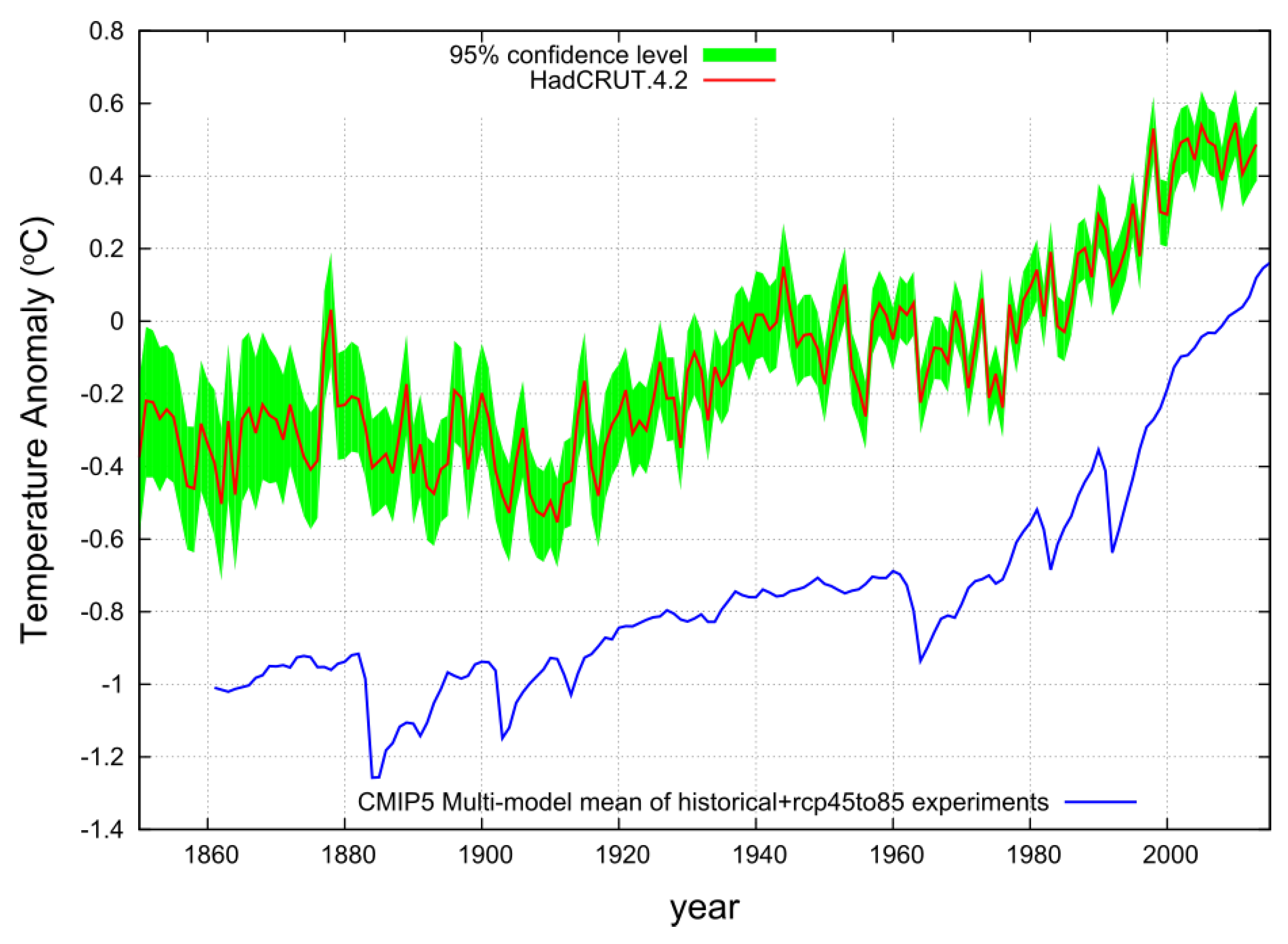
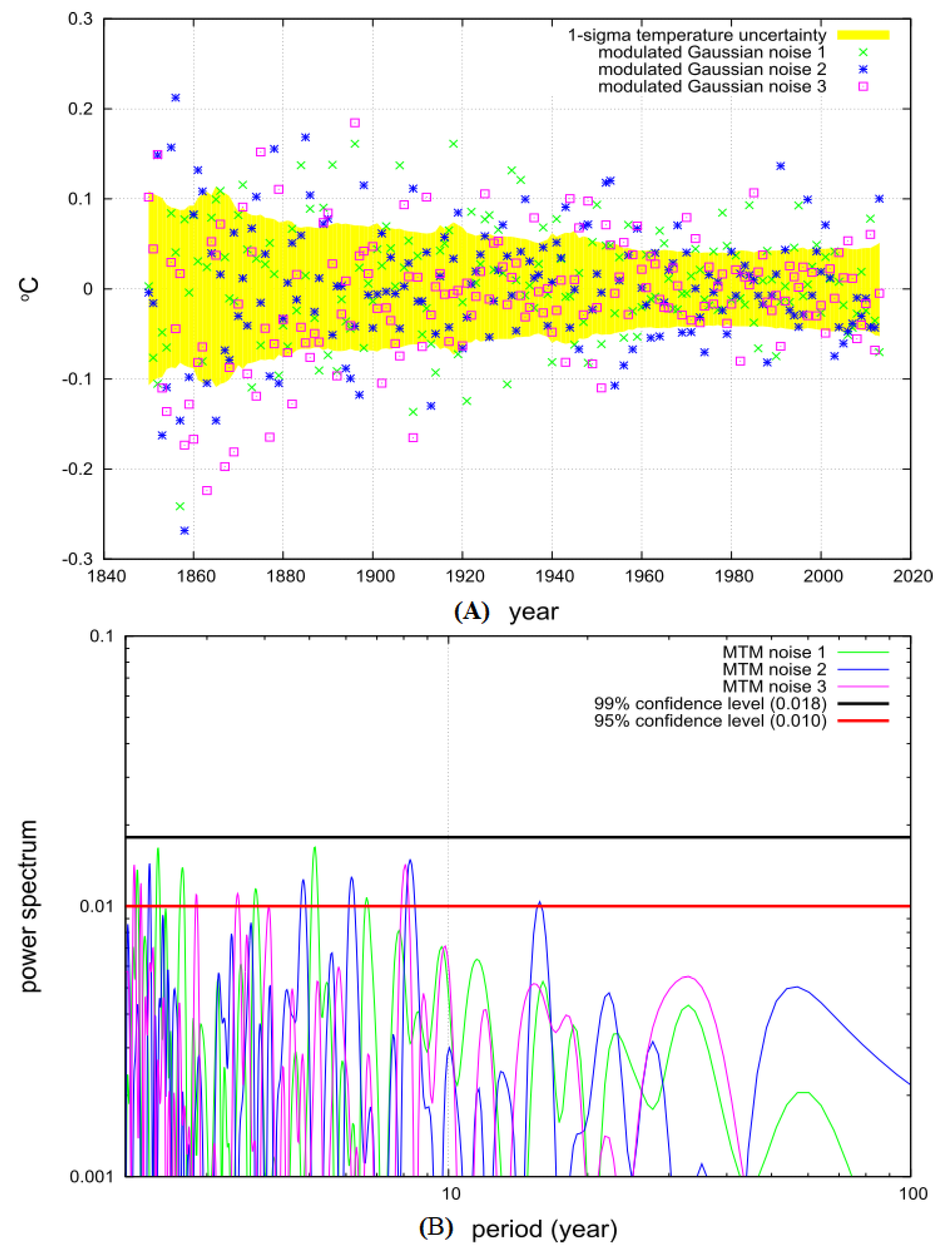
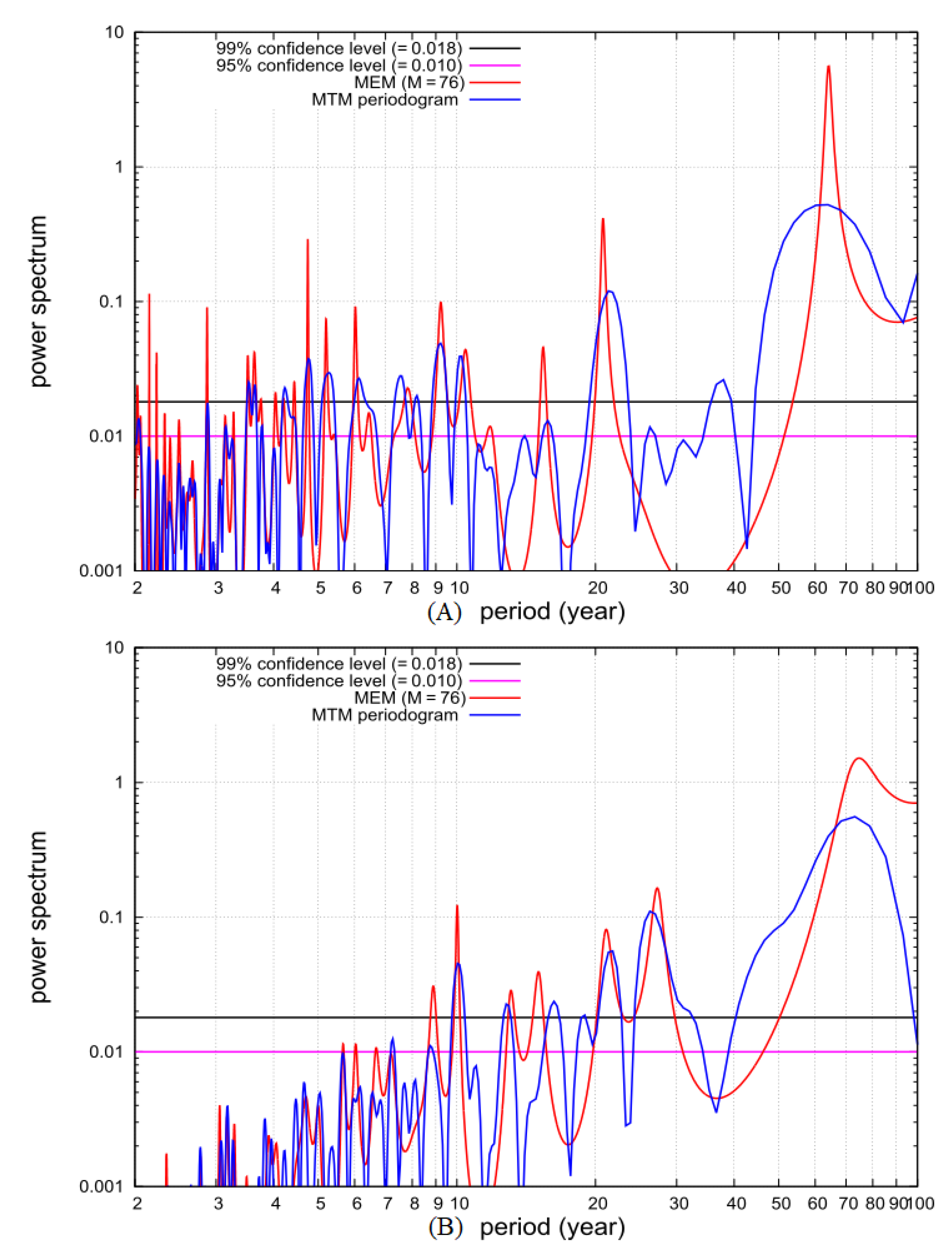
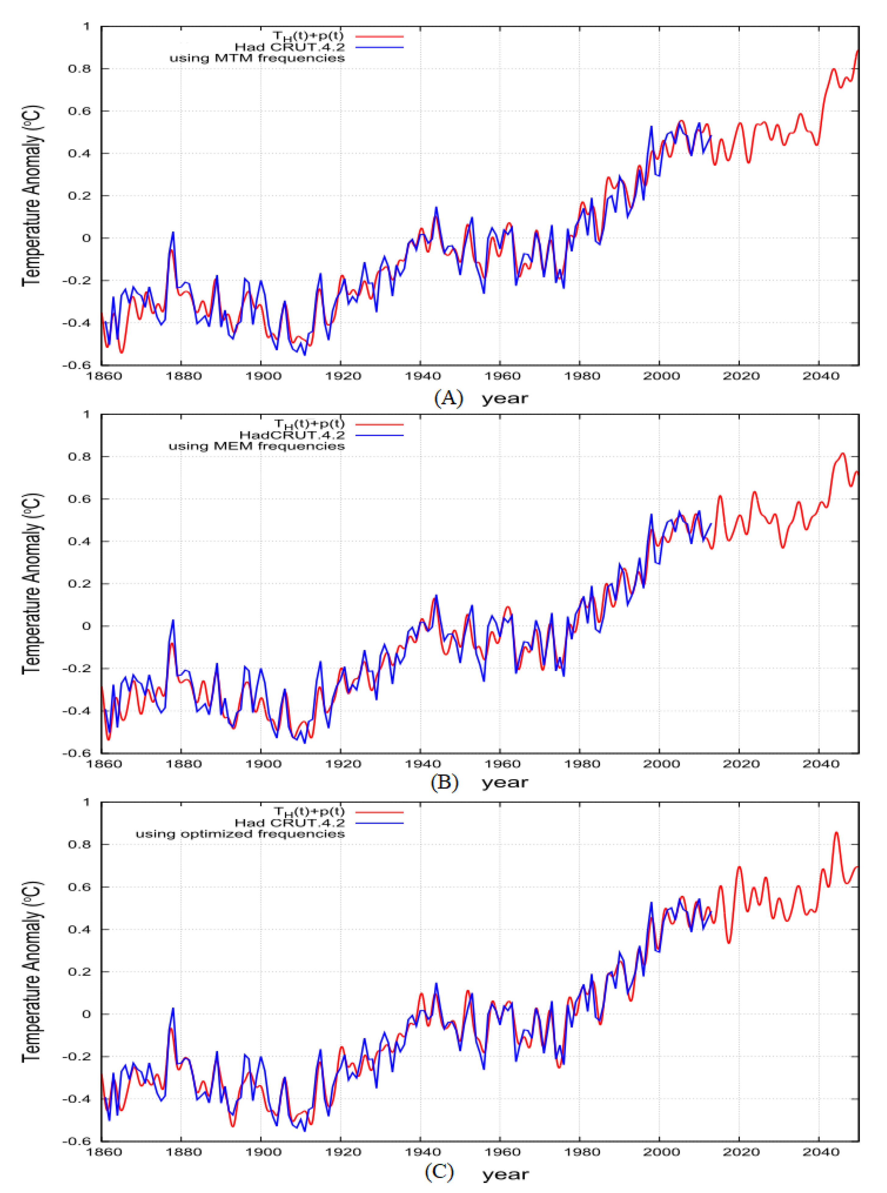
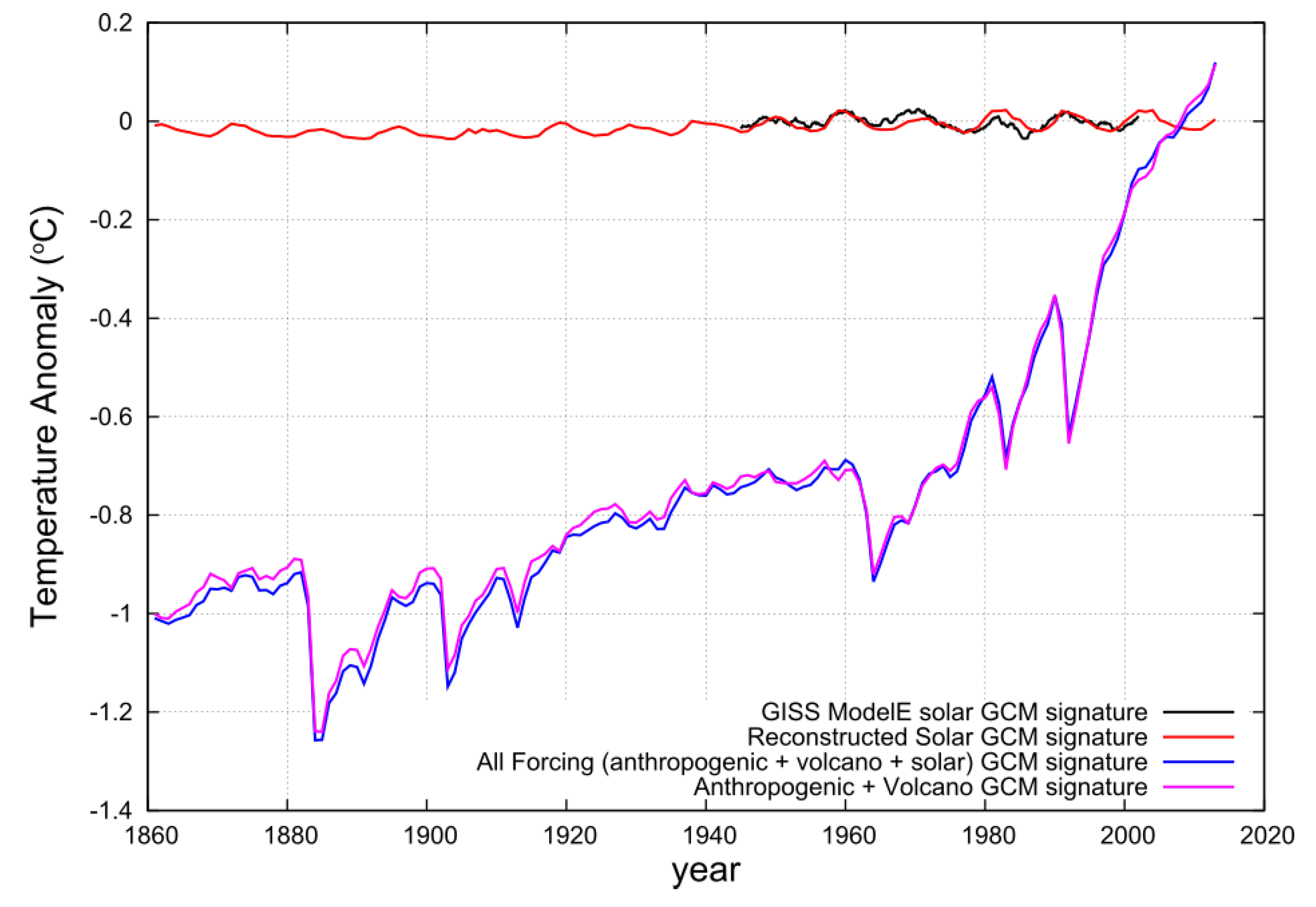
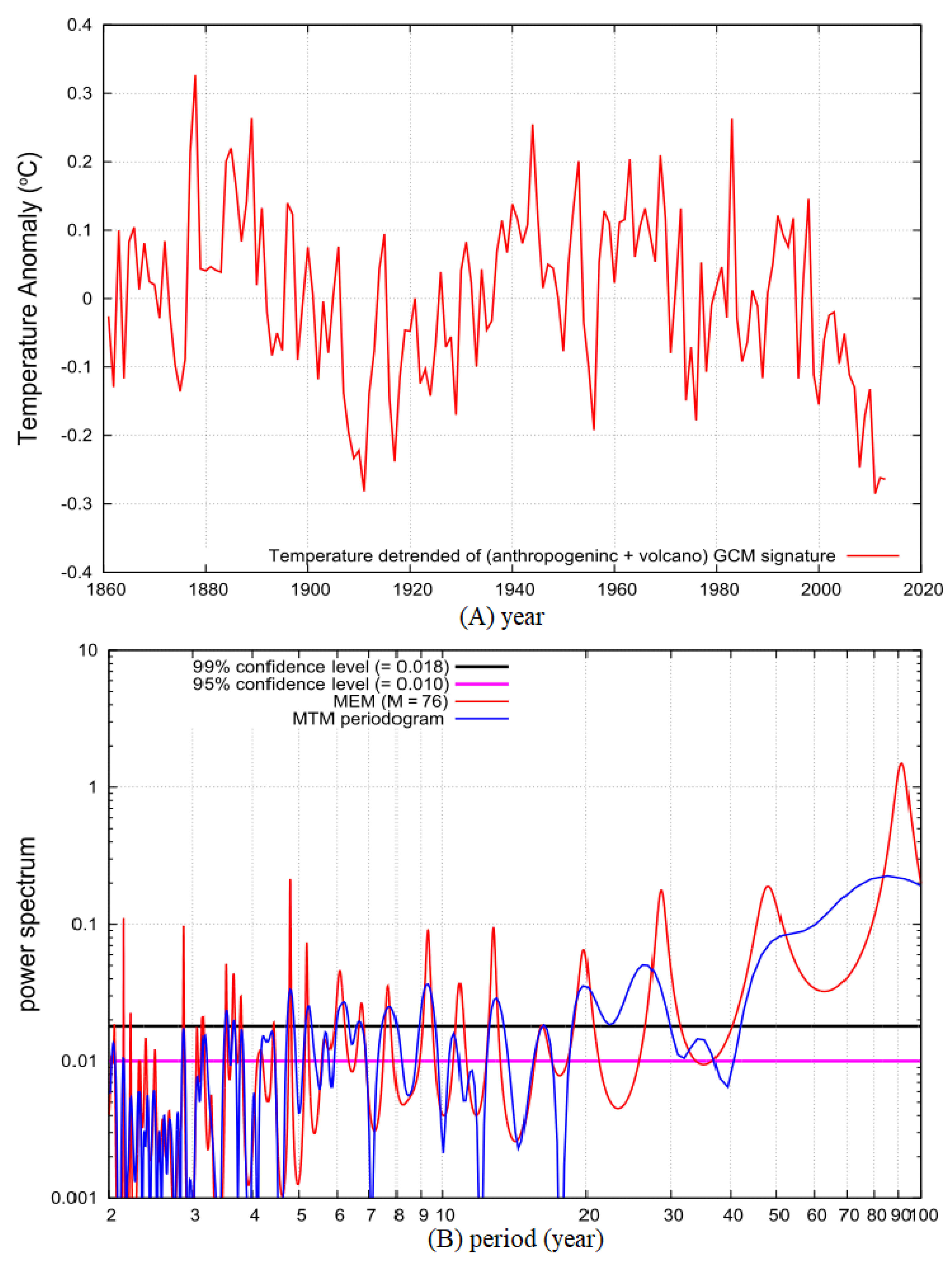
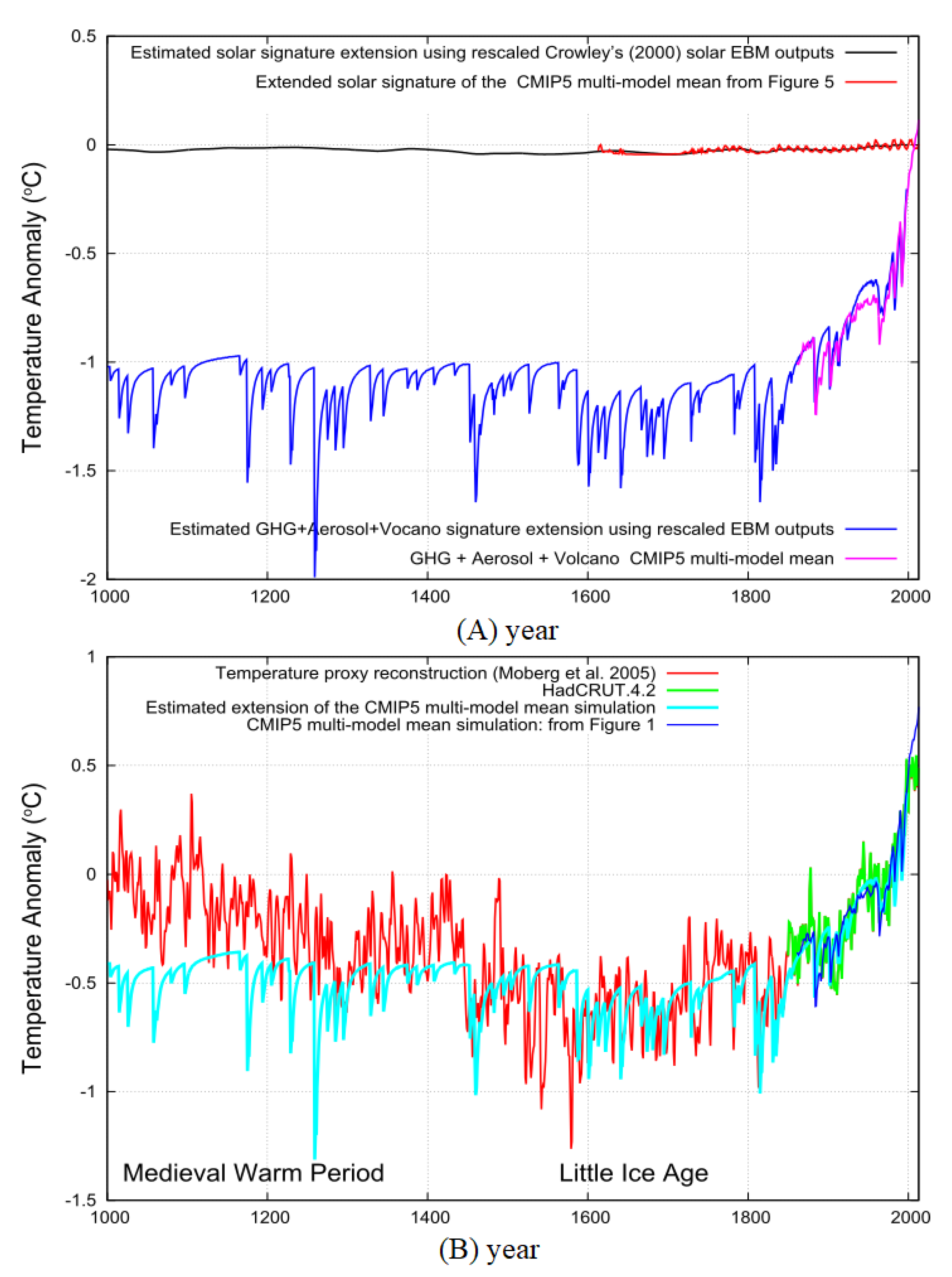
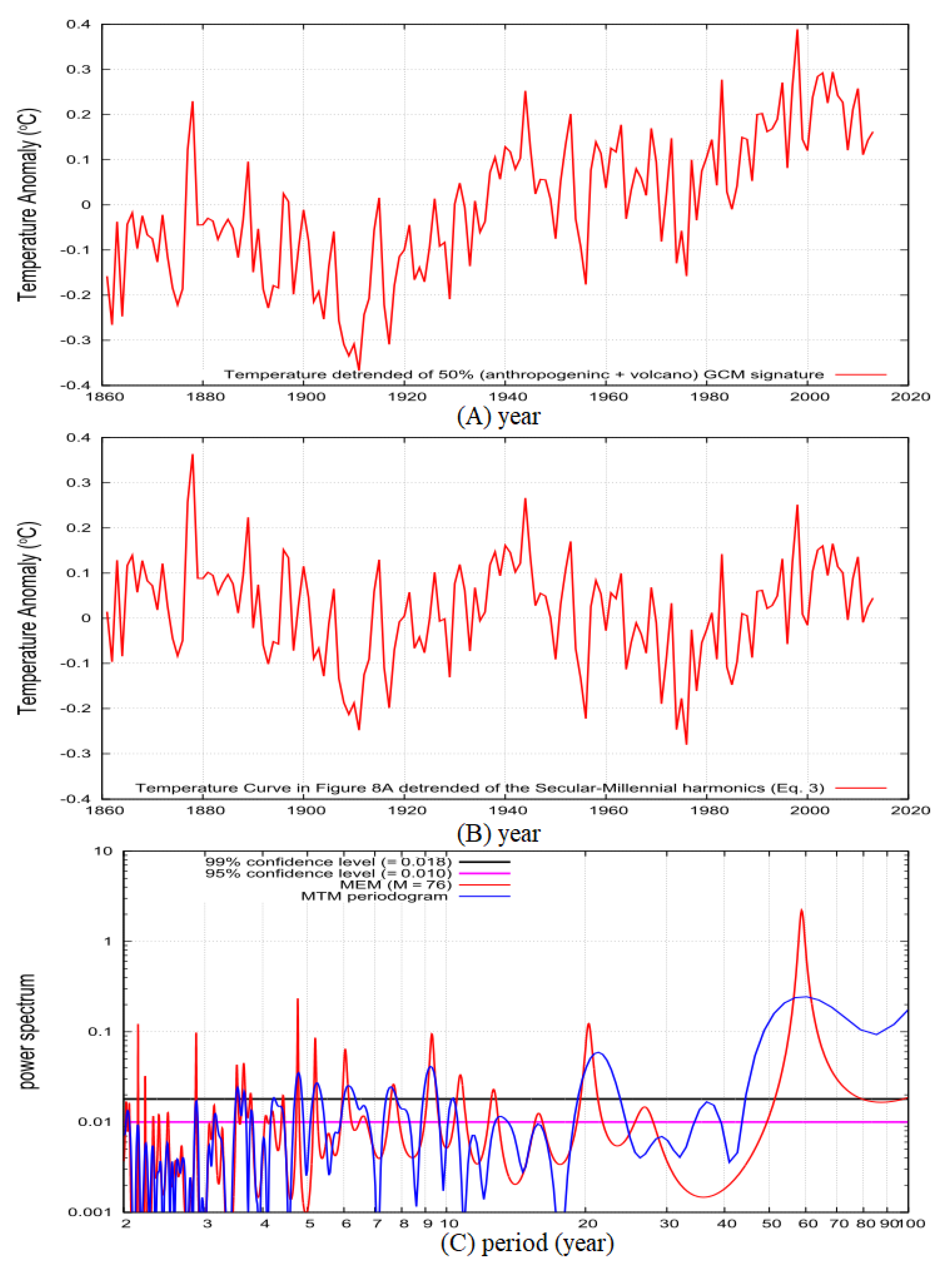
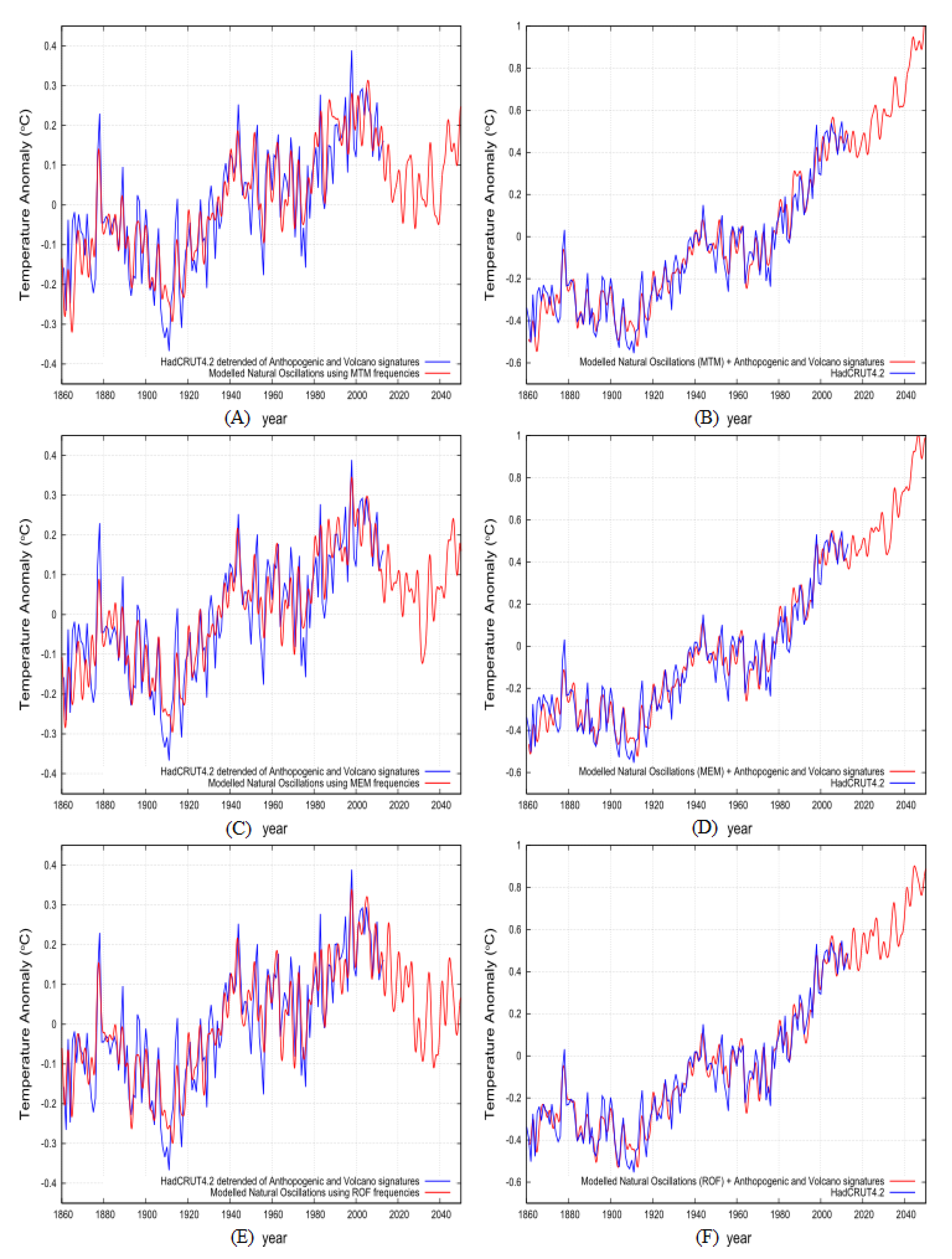
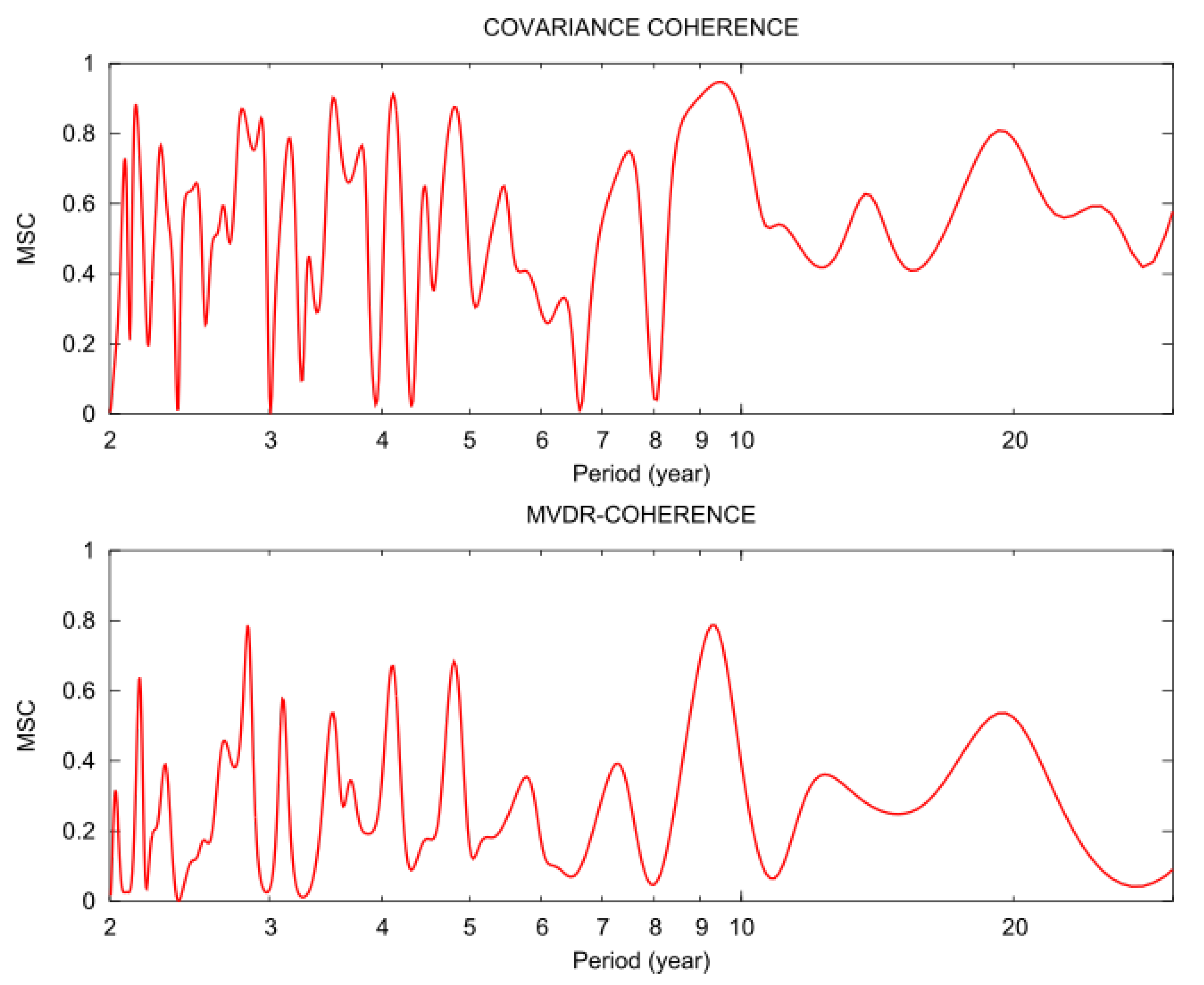
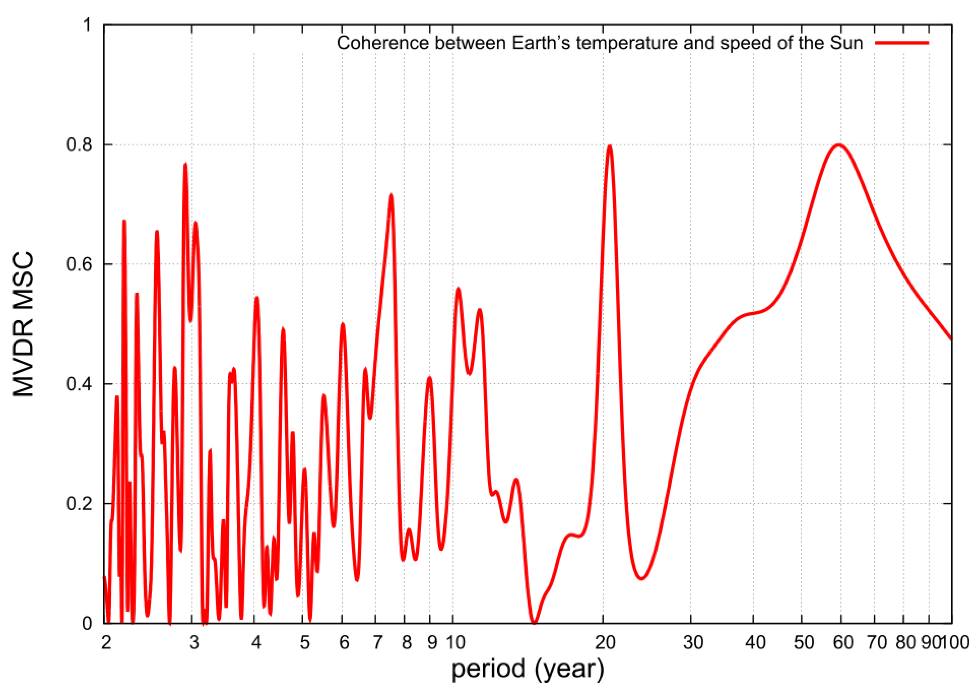
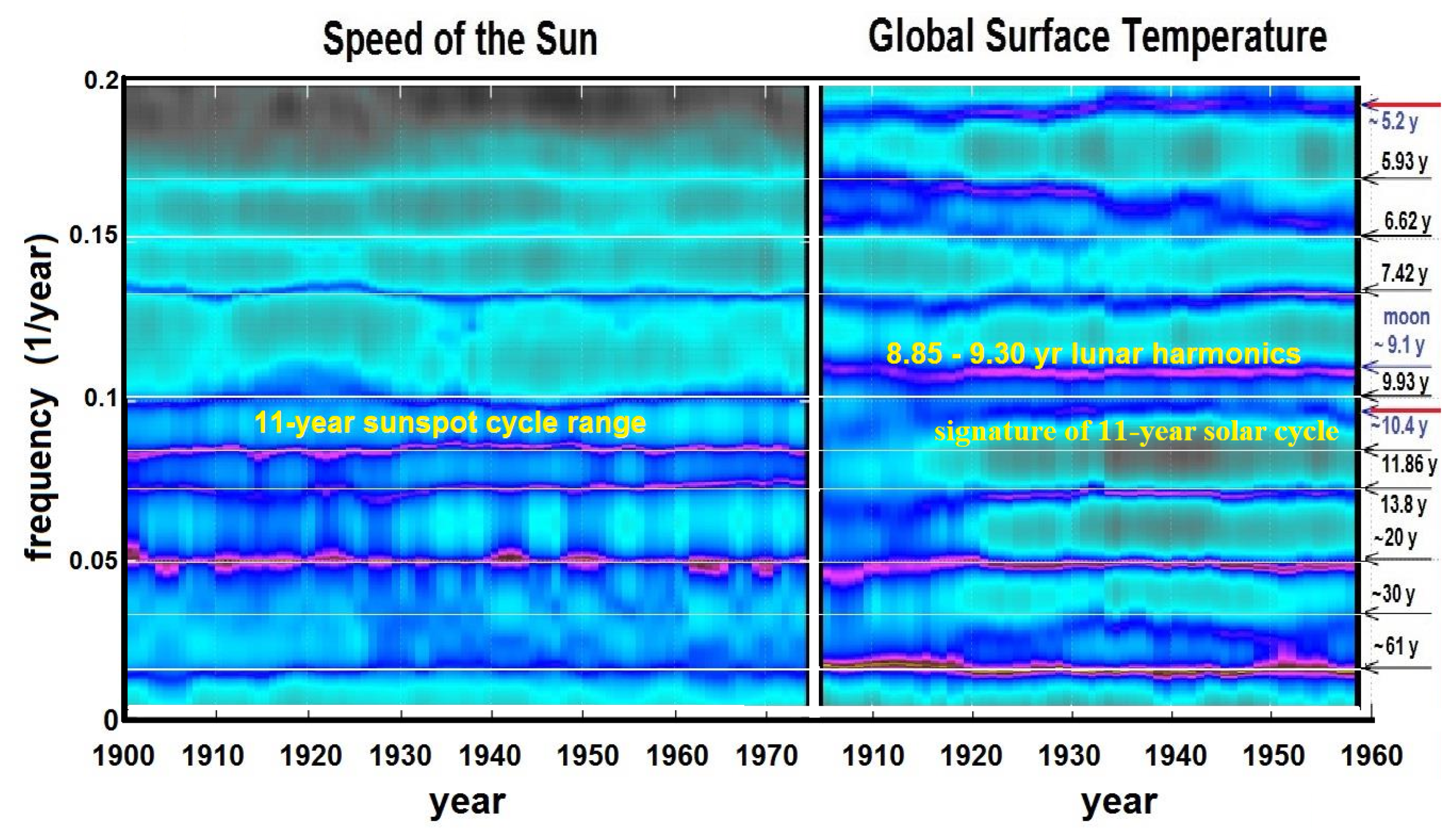
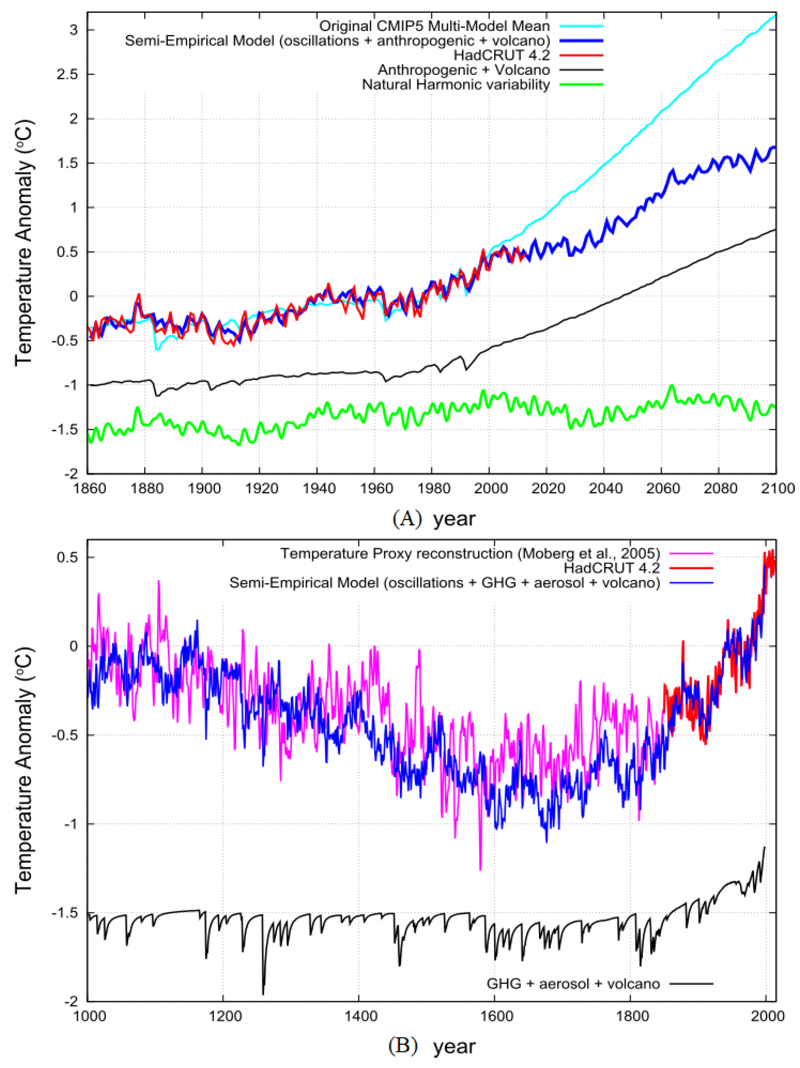
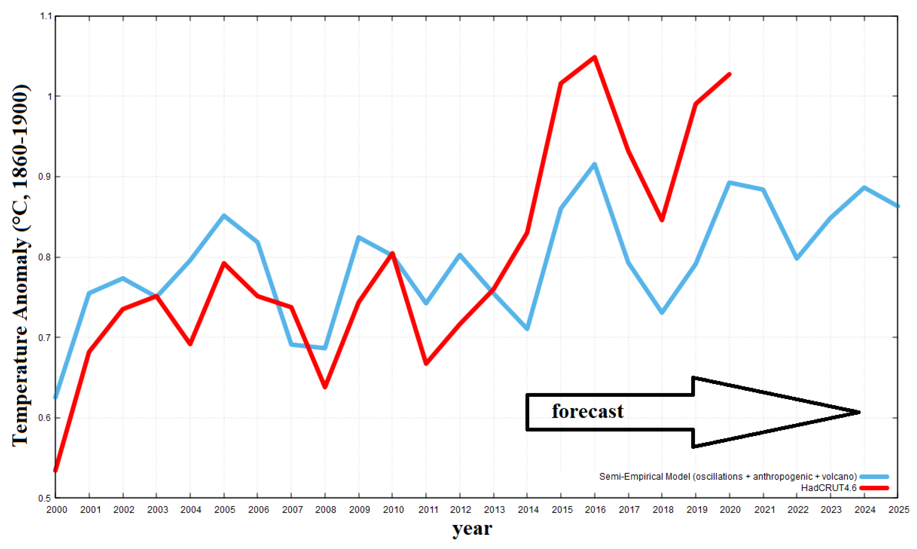
Table 1.
Regression coefficient of Equation (1) using the temperature MTM and MEM spectral peaks with a 99% confidence level depicted in Figure 3A and after a regression optimization of the frequencies. For a 153-year long sequence the spectral resolution is d yr and the statistical error in the reported frequencies is d yr. The three sets of frequencies are compatible within their statistical error. is the period, is the frequency, A is the amplitude of the sine wave and is the phase.
| MTM Spectral Peak Frequencies | MEM Spectral Peak Frequencies | Regression Optimized Frequencies | |||||||||
|---|---|---|---|---|---|---|---|---|---|---|---|
| () | () | (°C) | () | () | (°C) | () | () | (°C) | |||
| 62.11 | 0.0161 | 0.118 | 0.20 | 64.10 | 0.0156 | 0.122 | 0.16 | 65.79 | 0.0152 | 0.121 | 0.14 |
| 21.33 | 0.0469 | 0.042 | 1.00 | 20.75 | 0.0482 | 0.044 | 0.08 | 20.70 | 0.0483 | 0.046 | 0.10 |
| 10.24 | 0.0977 | 0.027 | 0.13 | 10.44 | 0.0958 | 0.025 | 0.97 | 10.21 | 0.0979 | 0.031 | 0.13 |
| 9.225 | 0.1084 | 0.038 | 0.45 | 9.234 | 0.1083 | 0.041 | 0.44 | 9.183 | 0.1089 | 0.039 | 0.50 |
| 8.190 | 0.1221 | 0.024 | 0.82 | 7.831 | 0.1277 | 0.015 | 0.38 | 8.190 | 0.1221 | 0.021 | 0.80 |
| 7.530 | 0.1328 | 0.024 | 0.66 | 7.645 | 0.1308 | 0.024 | 0.57 | ||||
| 6.131 | 0.1631 | 0.021 | 0.27 | 6.020 | 0.1661 | 0.027 | 0.61 | 6.254 | 0.1599 | 0.027 | 0.94 |
| 5.277 | 0.1895 | 0.025 | 0.33 | 5.200 | 0.1923 | 0.025 | 0.49 | 5.236 | 0.1910 | 0.029 | 0.42 |
| 4.762 | 0.2100 | 0.031 | 0.04 | 4.746 | 0.2107 | 0.033 | 0.10 | 4.773 | 0.2095 | 0.034 | 0.01 |
| 4.232 | 0.2363 | 0.017 | 0.46 | 4.202 | 0.2380 | 0.022 | 0.58 | 4.179 | 0.2393 | 0.026 | 0.65 |
| 3.644 | 0.2744 | 0.025 | 0.70 | 3.635 | 0.2751 | 0.024 | 0.73 | 3.628 | 0.2756 | 0.029 | 0.79 |
| 3.531 | 0.2832 | 0.023 | 0.89 | 3.516 | 0.2844 | 0.021 | 0.95 | 3.556 | 0.2812 | 0.028 | 0.79 |
| 2.876 | 0.3477 | 0.025 | 0.95 | 2.869 | 0.3486 | 0.025 | 0.02 | 2.875 | 0.3478 | 0.025 | 0.97 |
Table 2.
Regression coefficient of Equation (1) using the temperature MTM and MEM spectral peaks with a 99% confidence level depicted in Figure 8C and after a non-linear regression optimization of the frequencies. The three sets of frequencies are compatible within the spectral resolution of the analysis. is the period, is the frequency, A is the amplitude of the sine wave and is the phase. The is 0.06–0.07 °C.
| MTM Spectral Peak Frequencies | MEM Spectral Peak Frequencies | Regression Optimized Frequencies | |||||||||
|---|---|---|---|---|---|---|---|---|---|---|---|
| () | () | (°C) | () | () | (°C) | () | () | (°C) | |||
| 760 | 1/760 | 0.350 | 0.171 | 760 | 1/760 | 0.350 | 0.171 | 760 | 1/760 | 0.33 | 0.171 |
| 115 | 1/115 | 0.050 | 0.424 | 115 | 1/115 | 0.050 | 0.424 | 115 | 1/115 | 0.055 | 0.424 |
| 58.50 | 0.0171 | 0.086 | 0.26 | 58.82 | 0.0170 | 0.088 | 0.25 | 63.29 | 0.0158 | 0.091 | 0.17 |
| 21.32 | 0.0469 | 0.029 | 0.94 | 20.33 | 0.0492 | 0.033 | 0.08 | 20.33 | 0.0492 | 0.034 | 0.10 |
| 10.34 | 0.0967 | 0.023 | 0.024 | 10.72 | 0.0933 | 0.012 | 0.85 | 10.37 | 0.0964 | 0.025 | 0.00 |
| 9.225 | 0.1084 | 0.032 | 0.46 | 9.302 | 0.1075 | 0.033 | 0.37 | 9.19 | 0.1088 | 0.034 | 0.49 |
| 7.587 | 0.1318 | 0.020 | 0.61 | 7.680 | 0.1302 | 0.020 | 0.52 | 7.536 | 0.1327 | 0.020 | 0.65 |
| 6.131 | 0.1631 | 0.024 | 0.25 | 6.039 | 0.1656 | 0.027 | 0.51 | 6.010 | 0.1664 | 0.029 | 0.61 |
| 5.252 | 0.1904 | 0.026 | 0.39 | 5.198 | 0.1924 | 0.024 | 0.51 | 5.219 | 0.1916 | 0.026 | 0.44 |
| 4.785 | 0.2090 | 0.031 | 0.96 | 4.762 | 0.2100 | 0.031 | 0.03 | 4.787 | 0.2089 | 0.033 | 0.95 |
| 3.644 | 0.2744 | 0.024 | 0.70 | 3.640 | 0.2747 | 0.024 | 0.72 | 3.636 | 0.2750 | 0.027 | 0.75 |
| 3.531 | 0.2832 | 0.023 | 0.91 | 3.516 | 0.2844 | 0.021 | 0.96 | 3.554 | 0.2814 | 0.025 | 0.81 |
| 2.876 | 0.3477 | 0.025 | 0.96 | 2.871 | 0.3483 | 0.026 | 1.00 | 2.874 | 0.3480 | 0.025 | 0.98 |
Table 3.
The harmonic parameters of the astronomically optimized semi-empirical model. Here the 6 frequency and phases of the decadal to millennial harmonics were substituted with the theoretical values deduced from astronomical considerations. About the millennial cycle note that 760 year is not its period, see the full equation is Equation (7) and the explanation in the text. For the probable physical origin of the oscillations see Refs. [84,85,86,106].
| Semi-Empirical Optimized Frequencies | ||||
|---|---|---|---|---|
| Possible Origin | () | () | (°C) | |
| Solar/Planetary | 760 | 760 | 0.3228 | 0.1711 |
| Solar/Planetary | 115 | 115 | 0.0585 | 0.4239 |
| Solar/Planetary | 61 | 61 | 0.0859 | 0.152 |
| Solar/Planetary | 20 | 20 | 0.0334 | 0.148 |
| Sun Spots | 10.4 | 10.4 | 0.0241 | 0.020 |
| Solar-Lunar tidal | 9.3 | 9.3 | 0.0265 | 0.497 |
| Solar/Planetary | 7.463 | 0.1340 | 0.0216 | 0.711 |
| Solar/Planetary | 6.003 | 0.1666 | 0.0272 | 0.617 |
| Solar/Planetary | 5.238 | 0.1909 | 0.0260 | 0.409 |
| Solar/Orbital | 4.795 | 0.2086 | 0.0326 | 0.931 |
| Solar/Orbital | 3.633 | 0.2752 | 0.0276 | 0.767 |
| Solar/Orbital | 3.556 | 0.2812 | 0.0254 | 0.792 |
| Solar/Orbital | 2.874 | 0.3480 | 0.0247 | 0.975 |
Publisher’s Note: MDPI stays neutral with regard to jurisdictional claims in published maps and institutional affiliations. |
© 2021 by the author. Licensee MDPI, Basel, Switzerland. This article is an open access article distributed under the terms and conditions of the Creative Commons Attribution (CC BY) license (http://creativecommons.org/licenses/by/4.0/).
Share and Cite
MDPI and ACS Style
Scafetta, N. Reconstruction of the Interannual to Millennial Scale Patterns of the Global Surface Temperature. Atmosphere 2021, 12, 147. https://0-doi-org.brum.beds.ac.uk/10.3390/atmos12020147
AMA Style
Scafetta N. Reconstruction of the Interannual to Millennial Scale Patterns of the Global Surface Temperature. Atmosphere. 2021; 12(2):147. https://0-doi-org.brum.beds.ac.uk/10.3390/atmos12020147
Chicago/Turabian StyleScafetta, Nicola. 2021. "Reconstruction of the Interannual to Millennial Scale Patterns of the Global Surface Temperature" Atmosphere 12, no. 2: 147. https://0-doi-org.brum.beds.ac.uk/10.3390/atmos12020147
Note that from the first issue of 2016, this journal uses article numbers instead of page numbers. See further details here.