1. Introduction
Airborne particulate matter (PM) is a harmful atmospheric pollutant, due to the size and chemistry of the particles. A large fraction of it is anthropogenic; the main sources are industrial processes and production, including energy generation, traffic and transport, consumption and use of products, households, and agriculture. Anthropogenic aerosols contribute to climate change and have been linked to respiratory and cardiovascular diseases, lung cancer, and several other diseases [
2,
3,
4]. Knowledge of the chemistry of aerosols is vital for the understanding of health effects in indoor and outdoor environments. Aerosols loaded with heavy metals or other toxic elements contribute to various human health effects, ranging from cardiovascular and pulmonary inflammation to cancer and damage of vital organs even at the low concentrations found in ambient air. Generally, the smaller the size and greater the solubility of the particles, the higher the toxicity through mechanisms of oxidative stress and inflammation, prompted by the redox chemistry of these heavy metals. Deposition of metals causes contamination of crops for human and animal consumption—for example, leafy vegetables are particularly vulnerable to arsenic, lead, and mercury. Further details of health effects are given, e.g., in World Health Organization reports [
5,
6].
The European Union has developed an extensive body of legislation that establishes health-based standards and objectives for a number of pollutants in the air. The most important metric to monitor particulate air pollution is the mass concentration, or more specifically, the total mass of particles per unit volume of air with aerodynamic particle diameters smaller than 10 μm or 2.5 μm. These fractions are commonly referred to as PM
10 and PM
2.5, for which ambient limit or target values are established [
7]. EU regulations require quantification of the mass concentration of several chemical species in ambient aerosols, namely, elemental (EC) or organic (OC) carbon, selected anions and cations (such as ammonium, nitrates, and sulfates), as well as toxic elements and heavy metals (such as arsenic, cadmium, mercury, lead and nickel) with standard analytical reference methods [
8]. For the above-mentioned elements, measured as content in PM
10, the reference methods are sampling onto filters followed by leaching or digestion and atomic absorption spectrometry (AAS) or inductively coupled plasma optical emission spectrometry/mass spectrometry analysis (ICP-OES/ICP-MS) [
9,
10]. A Member State may also use any other methods, which give results equivalent to those mentioned above. For ICP-MS on filter samples, the EU data quality objective is 40% relative uncertainty for fixed or indicative measurements [
11], and typical lower limits of detection (LLOD) for regulated elements are (in ng/m
3) Pb: 0.5, Cd: 0.03, As: 0.2, and Ni: 1.1 [
10].
Ambient air quality monitoring is the task of air quality monitoring networks. Appropriate sampling equipment is installed at individual monitoring sites, the locations of which are determined by various factors, e.g., population exposure, spatial coverage [
12,
13]. It is common practice to take PM
10 filter samples on a 24 h-basis and to batch them for weekly chemical analysis.
In many countries, ambient air pollution and especially the level of particulate air pollution has decreased considerably in the last few decades. But there is evidence that current levels of air pollution still pose a considerable risk to the environment and to human health, and hence, the task of monitoring air quality remains for the foreseeable future [
5]. Air pollution monitoring networks may for indicative measurements substantially profit from the enhancement of air monitoring capacities by mobile methods to (a) enable measurements with an improved spatial resolution at low levels of air pollution close to the traditional methods’ LLOD; (b) monitor variations of pollution sources with higher time resolution, and (c) distinguish between local and remote pollution sources.
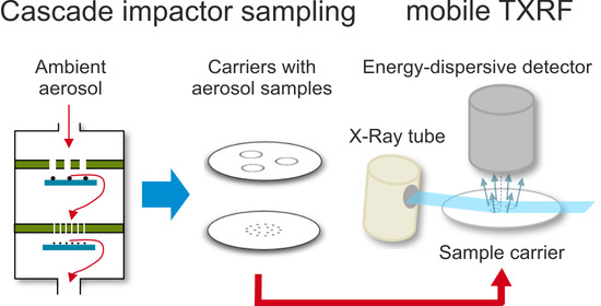
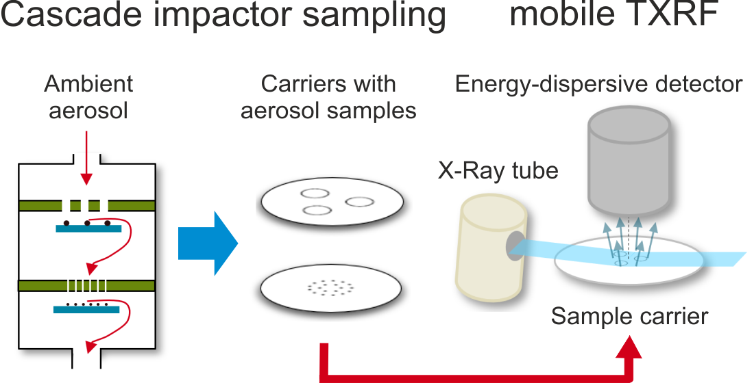
PM sampling by cascade impactors in combination with total reflection X-ray fluorescence (TXRF) spectroscopy [
14,
15] can provide such a mobile and flexible tool. This methodological approach was first proposed by Schneider, in 1989 [
16]. Injuk et al. (1995) [
17] did the first successful experiments which proved that compared to typical aerosol investigations using filters and/or digestion of particle-loaded filters, the sampling and analysis time, detection limits, and operating costs can be reduced considerably. TXRF analysis of airborne PM samples is since then frequently done by preprocessing (acid digesting, plasma ashing) of samples to only measure the deposit without interference from the sample’s material using lab-based TXRF spectrometers [
18,
19,
20,
21]. If robust, smooth, and clean carriers—adopted for particle collection in cascade impactors—are used, preprocessing or further treatment is not necessary, and the carriers can—as it is performed in this work—be analyzed directly on-site in a non-destructive way [
22,
23,
24,
25].
This paper reports on the first application of short-term cascade impactor sampling in combination with on-site TXRF analysis in the particle size range from ultrafine particles (UFP) up to 10 µm. This study aims to investigate (1) the proof of principles of this approach for short term elements analyses in ambient aerosols, (2) the traceability of field measurements to TXRF reference radiometrically calibrated TXRF serving as a reference, and (3) the demonstration of the comparability to the filter-based reference method ICP-MS [
26].
2. Experiments and Methods
To follow these aims, the following experiments were performed: Experiment 1: During an in-field measurement campaign in Cassino, Italy, conventional ambient aerosol PM
10 sampling on filters was performed over a number of runs of varying durations in accordance with the applicable standards. These filter samples were distributed to four laboratories (Laboratoire National de Métrologie et d’Essais LNE, France; National Physical Laboratory NPL, UK; Norwegian Institute for Air Research NILU, Norway and National Technical University Athens NTUA, Greece), and the collected element mass concentrations were determined by ICP-MS, following the standard EN14902:2005 [
10]. Experiment 2: Aerosol sampling on cascade impactor carriers was simultaneously performed at the same site, using a 13-stage cascade impactor (Dekati Ltd., Kangasala, Finland). These impactor samples were analyzed on-site by a mobile TXRF-spectrometer (Bruker S2 PICOFOX
®, Bruker Nano GmbH, Berlin, Germany). A second 9-stage cascade impactor (May) of a different design was also run simultaneously for comparison. These samples were analyzed afterward with a pre-calibrated TXRF spectrometer at the Centre for Energy Research (EK) in Hungary. Experiment 3: The S2-TXRF spectrometer was recalibrated specifically to analyze the cascade impactor samples against a physically traceable, reference-free X-ray spectrometry (XRS) arrangement [
27]. For this purpose, a set of calibration samples was generated in the lab using the 13-stage Dekati impactor and a nickel (Ni)-particle generator. This recalibration—which was not possible ahead of the field campaign for technical reasons—provides the traceability of the field campaign TRXF measurements to the reference of a well-defined amount of substance [
26].
The field campaign additionally provided useful information regarding the comparability of standard aerosol monitoring instrumentation. However, that is not in the focus of this paper, and will be published separately [
1].
2.1. TXRF
TXRF allows for the elemental analysis of the smallest particulate material quantities deposited on a carrier with a reflective surface. Monochromatized and collimated X-ray radiation, originating either from an X-ray tube or from a synchrotron storage facility, is used. The beam with known photon energy impinges on the carrier at a very small angle (<0.1°) beneath the critical angle of total external reflection and is totally reflected. The X-ray fluorescence photons produced in collected PM have element-specific characteristic energies and are detected using an energy-dispersive X-ray detector. Due to its short distance to the carrier, the solid angle of detection is optimal, and absorption by air is negligible. The main difference to conventional XRF is that under total reflection conditions, absorption, and scattering of the incident X-ray beam by the bulk substrate is drastically suppressed. Provided the deposition layer is sufficiently thin, the quantities of elements in it can be derived by the strengths of their respective elemental fluorescence signals using internal or external calibration standards, respectively applying a reference-free approach.
The determined absolute elemental mass, divided by the sampled air volume, provides the average mass concentration of an element in ambient air during a sampling period. Moreover, by using a cascade impactor with several stages, each with a defined particle size cut point, a particle size resolved elemental analysis is feasible. While TXRF spectrometers often are lab-based devices or integrated into a beamline, today, mobile benchtop spectrometers with in-field operation capability are available, which can be brought directly to the aerosol monitoring site for on-site elemental analysis. This option has several advantages: (a) The frequently occurring problem of samples contamination during handling, storage, and transport is minimized, the process is non-destructive, and the samples are available for subsequent research, (b) the portability of cascade impactors and TXRF spectrometers enables observation of local pollution hot spots on short notice without provision of lab capacities, (c) due to the high sensitivity short sampling intervals (few hours) are feasible and temporal variations of aerosol chemistry become observable, and (d) analysis can be repeated, and results can be quality assured and made physically traceable to a reference [
26].
2.2. (T)XRF Instrumentation
In the AEROMET [
1] field campaign, a commercial benchtop TXRF spectrometer (S2 PICOFOX
®, Bruker Nano GmbH, Berlin, Germany) was used—which, due to its lack of cooling media, its low weight, and its robustness, allow for a manual transport to enable an on-site analysis of the samples. The S2 operates in air and has an air-cooled Molybdenum (Mo) X-ray tube (max. 50 kV, 1 mA), a multilayer monochromator, and a Peltier-cooled XFlash
® Silicon (Si) Drift detector (Bruker Nano GmbH, Berlin, Germany) with 30 mm
2 detector area and energy resolution <149 eV at 100 kcps (Mo-Kα). The spectrometer comes in a 300 mm × 590 mm × 450 mm (height × width × depth) box, and the weight is 39 kg. It automatically operates a cassette with up to 25 manually fed acrylic glass carriers from the Dekati cascade impactor (see description below).
For comparison, field samples from the May impactor (see description below) have been measured with a lab-based TXRF system at EK [
28,
29]. It comprises a 50 W microfocus Mo-anode X-ray tube (Petrick, Bad Blankenburg, Germany), a Mo/Si multilayer monochromator (AXO, Dresden, Germany) for Mo-Kα excitation operated at 50 kV and 1 mA, and for our purposes, a 7 mm
2 silicon drift detector (KETEK, Munich, Germany) was used. The AXIL software [
30] was used to evaluate X-ray spectra. Typically, 3000 s counting time is used for a Si wafer with a moderate load of aerosol particles. Measurements are performed in the air.
Reference-free XRS was applied at the four crystal monochromator (FCM) beamline in the laboratory of the German national metrology institute PTB at the BESSY II electron storage ring in Berlin, Germany [
27,
31].
This beamline provides monochromatized X-ray photons in the energy range from around 1.7 keV up to 10 keV. The radiometrically calibrated instrumentation allows for a reference-free quantification [
26] of elemental masses in a sample, e.g., particulate matter collected on a cascade impactor carrier. In an ultrahigh-vacuum (UHV) chamber, a 9-axis manipulator precisely tunes the incident angle θ between the X-ray beam and the sample surface. The fluorescence radiation emitted from the sample is detected using a calibrated silicon drift detector (SDD) [
32], which is placed in the polarization plane and perpendicular to the propagation direction of the incident X-ray beam to minimize radiation scattered elastically or inelastically from the sample. The incident photon flux is monitored using a calibrated photodiode. The spectra can be deconvoluted using the known detector response functions [
31] for the relevant fluorescence lines and background contributions, which are mainly coherent and incoherent scattering, and to a lower extent, Bremsstrahlung from the substrate. The resulting count rates for the fluorescence line of interest are normalized with respect to the sine of the incident angle θ, the incident photon flux, the effective solid angle of detection Ω/4π, and the detection efficiency of the SDD for the respective fluorescence photons to derive the emitted fluorescence intensity which can be thereafter converted to a mass deposition using the Sherman equation [
33].
2.3. Cascade Impactors and Collecting Substrates
Sampling was performed with two impactors: The commercial Dekati DLPI 10
® (Dekati Ltd., Kangasala, Finland) low-pressure cascade impactor samples at a fixed rate of 10 L/min on 13 stages with aerodynamic cut points at 0.03, 0.06, 0.1, 0.2, 0.3, 0.4, 0.7, 1.1, 1.8, 2.7, 4.3, 7, and 10 µm. In each stage, circular jets generate rotationally symmetric deposition patterns on the carriers, which consist of small dots, arranged in up to four concentric rings (see
Figure 1 below).
Each stage has its characteristic pattern, whose maximum lateral extension of 9 mm fits almost, but not perfectly to the excitation zone width of the S2 TXRF spectrometer. The stages’ carrier holders have been redesigned by BAM to hold commercially available acrylic discs (30 mm diameter, 3 mm thickness) as carriers. These standard TXRF carriers are for single-use and come with adhesive protection, which avoids contamination during mounting. Quartz discs would be advantageous for TXRF, but are too costly for single-use, and cleaning is quite an elaborate process. When operating in a lightweight tent or in a mobile measuring station, dismounting of loaded carriers and mounting of a set of fresh ones takes altogether 0.5–1 h. A standard counting time of 1000 s per carrier sums up to 3.6 h for a TXRF-scan of a complete Dekati impactor set (13 carriers). Carriers loaded in shorter periods can easily be stored temporally before analysis on the same day or overnight.
The May impactor [
34] was extended by EK to 9 stages (aerodynamic cut points at 0.07, 0.18, 0.29, 0.57, 1.13, 2.25, 4.5, 8.9, and 17.9 µm), and the sampling rate is 16.7 L/min [
29]. Each stage establishes a jet through a slit nozzle of 50 mm length. The slit width decreases with the stage cut point. The deposition pattern on each of the carriers is a thin centric stripe with varying widths of 0.1 mm (stage 9) to 1 mm (stage 3). Different types of carriers are applicable: Round or square Si-wafers have a very smooth surface, which is preferable for TXRF. They are cleanable, reusable and a quick manual change of carriers at the sampling site is possible. Quartz discs or acrylic discs with 30 mm diameter and 3 mm thickness can, e.g., also be applied, and carrier holders can be designed with high adaptability to other carrier shapes.
Traceable quantitative element standards for TXRF calibration can be applied to all types of substrates. As the collected samples were intended to be partially available for different (micro)analytical investigations, no pre-treatment of the May impactor’s Si carriers was performed onto stages 3–9, which cover a PM diameter range of 0.07 to 9 µm. The collection of particles larger than 10 µm was not of interest, therefore acrylic substrates used at stages 1 and 2 were not further analyzed. The Dekati carriers were prepared by pipetting dried residues of 50 ng of an aqueous Yttrium standard solution (Merck, Germany) in the center. The Y masses on the prepared carriers were measured before use, and carriers showing more than 10% deviation from the mean were rejected.
An upper limit for quantitative TXRF analysis is given by self-adsorption in the sampled material, which may impair the absolute quantification of elements [
35,
36,
37]. Therefore, the maximum collection time on a set of carriers was several hours at the prevailing moderate average air pollution level of PM
10 below 20 µg/m
3 in Cassino.
Particles in an impactor may, due to their high kinetic energy, bounce off when they impact on the carriers’ surfaces before they are eventually deposited in stages downstream. While the total deposited mass is hardly affected, this leads to a bias in the particle mass size distribution in the impactor. Particle bounce-off depends on factors, such as the carriers’ surface properties and precoating, loading effects, and several more [
38]. A standard measure to minimize re-entrainment from the carrier is the application of an adhesive. During the field campaign, the acrylic carriers for the Dekati impactor were precoated with sprayable metal-free Apiezon
® vacuum grease, following the procedure recommended in the manufacturer’s manual. For the May impactor, only the acrylic carriers at stages 1 and 2 (aerodynamic cut-points 17.9 and 8.9 µm) were coated to minimize the bounce-off of large particles.
2.4. PM10 Sampling
For aerosol sampling and ICP-MS analyses, the following PM10 aerosol samplers with impactor inlets and filters with 47 mm diameter were used and run simultaneously: Two PM10 samplers (Zambelli S.r.l., Bareggio, Italy) working at a nominal fixed flow rate of 1.0 m3/h (according to the US standard US-EPA 40 CFR) and equipped with low porosity cellulose nitrate filters (Whatman, Maidstone, UK, pore size 0.45 μm); two PM10 samplers (LVS3, Leckel, Berlin, Germany) with a nominal fixed flow rate of 2.3 m3/h (according to the European standard EN 12341:2014) and equipped with low porosity polycarbonate filters (Whatman, Maidstone, UK, pore size 3 μm).
2.5. ICP-MS Spectroscopy
The PM10 aerosol samples from the field campaign were distributed to the following AEROMET project partner laboratories for ICP-MS analysis: National Technical University Athens NTUA, Athens, Greece; the National Physical Laboratory, NPL, Teddington, UK; Norwegian Institute for Air Research NILU, Kjeller, Norway and Laboratoire national de métrologie et d’essais LNE, Paris, France. Methodological details are described briefly below:
NTUA: The ICP-MS-System is an Agilent 7700 ICP-MS with Helium (He) mode, with which an external calibration curve was generated for all analytes. A second ICP-MS instrument Thermo ICAP Qc (Thermo Fisher Scientific, Waltham, MA, USA) was also used with internal standardization (Sc for V, Mn; Ge for Cr, Ni, Cu, As; In for Cd; Ir for Pb) and external calibration. A multi-element ICP Quality Control Standard solution (QCS-27, ChemLab, Zedelgem, Belgium, CL01.13612.0100) of 100 mg/L for each element in 2 to 5% nitric acid (HNO3) with traces of hydrofluoric acid (HF) was used for the preparation of the working standard solutions in a concentration range of 0–50 μg/L. For the method validation (for both instruments) reference materials NIST 2583 and NIST 2584 (trace elements in indoor dust) were measured under similar conditions and underwent the same sample preparation procedure. A very good agreement with the certified values was achieved for all the elements investigated.
NPL: The ICP-MS-System is an Agilent 8800 ICP-QQQ-MS (Agilent, Santa Clara, CA, USA). The calibration utilized up to 6 gravimetrically prepared calibration standards prepared from stock solutions certified to ISO 17034 (Romil, Waterbeach, UK). The working calibration standards were prepared in nitric acid and hydrogen peroxide to match the matrix of the digested sample solutions. Analyte responses were normalized against an appropriate internal standard element (Sc for V, Cr; In for Mn, Fe, Cu, Zn, Cd; Y for Ni, As; Bi for Pb). The single quad method used He mode for Fe; for all other analytes, no gas was used for interference removal. Sample digestion and ICP-MS methods are regularly validated by processing Certified Reference Materials, including NIST 1648a (urban PM, NIST, Gaithersburg, MD, USA) and NIES no. 28 (urban aerosols, NIES, Tsukuba, Japan). For every analytical run, a QC solution is analyzed, containing the analytes of interest prepared from independent metal stocks from the calibration standards to verify their accuracy. NPL supplied results with full expanded uncertainties (k = 2) calculated in accordance with the Guide to the expression of uncertainty in measurement [
39].
NILU: The ICP-MS-System is an Agilent 7700x (Agilent, Santa Clara, CA, USA). Internal standard 100 ng/mL In made from a certified stock solution traceable to NIST (Spectrascan and Teknolab AS, Ski, Norway), added to the sample line at a constant rate. External calibration by diluted multi-element mixes and single element solutions (Spectrascan and Teknolab AS, Ski, Norway), traceable to NIST. All calibration standards were prepared in 10% (v/v) s.p HNO3 to match the sample matrix. The calibration curves were verified by analyzing control samples prepared in 10% (v/v) s.p HNO3 from certified multi-element mixes (Inorganic Ventures, Christiansburg, USA) traceable to NIST, before filter samples were analyzed.
LNE: The ICP-MS-System is a Thermo iCAPQ ICP-MS (Thermo Fisher Scientific, Waltham, MA, USA) in Kinetic Energy Discrimination (KED) He mode. For the external calibration, multi-elemental calibration solutions were prepared by gravimetry using high purity metals or salts traceable to the SI. Verification of the prepared standards was carried out using a commercial certified reference material (Certipur®, MERCK, Darmstadt, Germany) traceable to NIST.
Regarding PM
10-filters sample preparation and digestion protocols: NPL and LNE digested the entire filters as supplied. NTUA digested two quarters from cut filters in most cases (in a few cases only 1 quarter was digested). NILU digested one half from cut filters. Both corrected their results for the portions analyzed. NPL, NTUA, and LNE adopted very similar digestion protocols based on the standard EN 14902:2005 [
10]. Filters were digested in hydrogen peroxide (~30%) and suprapure nitric acid (~70%). Microwave programs achieved temperatures up to 220 °C held for 25/30 min. Digested filter solutions were diluted to 50 mL with ultrapure water. NILU extracted each filter portion in a mixture of 1 mL supra pure nitric acid and 2 mL deionized water. Digestion of the filter samples was performed with a microwave high pressure reactor, the highest temperature was 250 °C, held for 15 min. After cooling, the samples were diluted to 10 mL by deionized water.
2.6. TXRF Calibration and Traceability
In many TXRF applications, it is sufficient for an absolute element mass quantification in samples to calibrate a spectrometer against traceable and certified (multielement) standards, i.e., samples containing known quantities of reference element masses on a narrow spot in the carrier’s center. This simple approach is, however, not applicable for samples from cascade impactors like the Dekati for the above-mentioned individual and complex deposition patterns with varying lateral extensions and coverage. These differ from stage to stage, and this has a crucial impact on the quantification of elements in the deposit [
36]. There are no robust field-suited techniques that prepare carriers with element standards in patterns mimicking the deposition patterns. Corrections must be applied to compensate effects, such as incomplete or inhomogeneous excitation of the deposit, and also lateral efficiency in the fluorescence detector. While a suitable correction algorithm for each of the impactor stages was not available, a strategy was pursued of experimentally comparing the quantification of the S2 spectrometer to the SI traceable, reference-free XRS using synthetic samples which resemble the patterns on the Dekati carriers to derive stage-individual correction factors. A set of 12 calibration samples, i.e., stages 1 to 12, which represent the PM
10 fraction of the Dekati impactor, was generated in the lab by collecting aerosolized Ni particles with a broad size distribution for approximately 10 min on acrylic disc carriers at a standard sample flow of 10 L/min. The aerosol was generated from an aqueous solution of Ni(II)-acetate (1.0 g/L) in an atomizer (ATM 220, Topas, Dresden, Germany) and completely dried upstream of the collection in a diffusion dryer (type 3062, TSI, Shoreview, USA). The reference-free XRS measurements of this set were made at 10 keV incident photon energy.
Given the rather large deposition area on the carriers and the small beam focus of the synchrotron radiation beam, lateral scanning of the carriers’ surfaces was required. A shallow incidence angle of 10° was selected as a good compromise between the spatial resolution in the scanning measurements and enhanced excitation of XRF in the PM and reduced background contributions from the substrate. These settings enabled a reliable quantification of the mass deposition at each measurement position, and the mapping mesh width could be increased in one dimension, due to the beam projection to optimize the measurement time. During the lateral scanning measurements, the step size in the horizontal and vertical directions was chosen in agreement with the (projected) beam dimensions. The 12 mm × 12 mm scanning area was centered on the deposition pattern. Detected element masses were calculated using a two-dimensional numerical integration within a centered square region of interest. The mass depositions outside the region of interest were also quantified and used as an estimate for a background correction factor, considering possible contamination of the carriers’ surfaces. The quantified Ni masses ranged from few nanograms to several thousand nanograms depending on the impactor stage.
The May impactor samples have only been analyzed with the lab-based TXRF spectrometer at EK. For calibration, linear arrays of standard solutions (Merck IV multielement, 23 elements, and several single-element standards) have been deposited on the centerline of the carriers, which consisted of Si wafers with an edge length of 20 mm, by a nanoliter injector (WPI, Sarasota, FL, USA)) and the sensitivities relative to chromium were determined. Sensitivities of elements which are not contained in the measured standard solutions were obtained using polynomial interpolation. The absolute mass determination of the spectrometer was then calibrated using 4 ng and 8 ng (relative uncertainty ± 5%) Cr standards prepared as pads of respectively 50 nm and 100 nm height arranged along the carrier centerlines. The stripe width was 350 µm. These dimensions are similar to those of aerosol deposits. The procedure is described in detail in the literature [
40,
41].
2.7. Aerosol Sampling Scenario
The sampling site in Cassino (a middle town in Central Italy, 30 km distance from the Tyrrhenian Sea) was a covered balcony (dimensions 3.9 m × 7.5 m) on the second floor of a building, owned by the University of Cassino and Southern Lazio. The building is located in the urban area and a two-ways single lane street with free flow traffic conditions characterized by a traffic density of approx. 24 vehicles/min with a mean velocity of about 30–40 km/h is 20 m away. The street can be considered a wide canyon characterized by large openings on the walls. The weather conditions during the campaign in September 2018 were stable with negligible precipitations. In the first half of the campaign, the average temperature was 24.9 °C at 72.2% relative humidity with prevalently southernly low winds. In the second half, a cold front was causing a lower average temperature of 19.5 °C at 47.1% relative humidity, and with slightly stronger shifting winds from S, NW, and E. Referring to data from the nearby Environmental Protection Agency measuring station, the 24-h average PM10 dropped from approximately 22 μg/m3 at the beginning of the first week to 12 μg/m3 afterwards.
2.8. Field Campaign Sampling Schedule
The particulate matter load of samples for quantitative TXRF analysis had to be limited to avoid self-absorption, which may have impaired the absolute quantification of elements. The collection time for TXRF samples was, therefore, restricted to less than 1 day, considering the moderate PM
10 level in Cassino during the campaign. On the other hand, ICP-MS profits from higher analyte concentrations on the filters. This contrast has been solved the following way: Nine sampling periods, listed in
Table 1 below, with different durations, were performed. In each run 4 PM
10 filter samples (one in each PM
10 sampler) were collected simultaneously. In runs 1, 2, 3, 6, and 9 samplings with the cascade impactors agreed timewise exactly with the filter sampling. In runs 5, 7, and 8, Dekati impactor sampling periods were shorter, but added up to the respective filter sampling duration. During the interruptions needed for impactor carrier exchange, the filter sampling was interrupted too. This directly compares the element mass concentrations of PM
10 filters with those of the cascade impactor samples after correction for the different sample flow rates. During run 4—actually the longest run—a technical malfunction impeded the simultaneous operation of PM
10 samplers and cascade impactors.
3. Results
3.1. Results from Experiment 1
In
Table 2 the ICP-MS mass concentrations of the analyzed elements are reported. The data represent the average values and relative standard deviations calculated from the data provided by all four laboratories. Since for several elements filter background contamination (including high element concentrations on the blank filter and significant variability) was detected, results are given without blank filter subtraction.
As it turned out, there is generally satisfactory agreement, i.e., the RSD is significantly below 50%, between the labs for most of the elements analyzed. However, there are clear instances of very high discrepancy, especially for the elements Cr, Ni, Cd, and Pb in runs 1, 2, 3, 5, and 9. The obvious reason for this could be unexpected high filter contaminations. Several blank filters of both types—polycarbonate and cellulose filters—have been analyzed, revealing very high contaminations of Cr, Mn, Fe, Cu, Zn, and in some cases, Pb. Moreover, these contaminations had high variations, and therefore, a prediction of representative background levels and proper background corrections seemed impossible. It is fair to conclude that the observed significant variations between the results from the different laboratories were much higher than would be suitable for trace metal analysis for these metals. It also seems likely that filter contamination is the reason for the discrepancies between the sample results in several of the runs. Further reasons for the discrepancy could be attributed to the sampling times, sampling rates, and air volumes. Samples sent to LNE and NTUA were sampled at a flow rate of 1 m3/h, but those sent to NPL and NILU were sampled at 2.3 m3/h, resulting in a higher volume of air being sampled and a larger PM deposit. While the average measured concentration should still be the same, the samples with the larger deposits provide (i) a greater chance of collecting analyte quantities above the ICP-MS detection limit and (ii) a more accurate average, because a larger air volume was sampled. Indeed, a better agreement between results was seen when larger air volumes were sampled. We decided to consider only runs 6, 7, and 8 for the comparison with the TXRF analysis results. These runs were relatively long and revealed consistently low variations in the measured element concentrations between the labs, i.e., relative standard deviations below 30% (slightly higher levels were seen to be tolerable, however, for Ni and As in run 7.
3.2. Results from Experiment 2
The loaded carriers from the Dekati impactor were analyzed during the field campaigns in situ with the S2 TXRF-spectrometer using monochromatic Mo Kα excitation at 17.5 KeV and 1000 s as standard measurement interval and with the manufacturer’s software (PICOFOX 7.8.2.0, Bruker Nano GmbH, Berlin, Germany). Especially for multi-element samples, strong overlaps of individual fluorescence peaks in the spectrum occur because of the line diversity and the finite detector resolution. For quantification, the Bruker TXRF software applies a non-standard deconvolution routine (SuperBayes), which uses measured mono-element profiles for the evaluation of peak intensities [
42].
While preliminary results were initially obtained using the 50 ng Y standard for a comparison of element mass concentrations during the campaign, all data were corrected after recalibration of the S2 TXRF spectrometer (see results of experiment 3 below). For comparison of the total element mass concentrations in the PM
10-fraction, only stages 1 to 12 of the Dekati impactor have been considered. Stage 13 (cut point 10 µm) was not included because there was a 50% chance that particles >10 µm in diameter would be collected, which would bias the comparability to the PM
10 filter samples.
Table 3 reports the results for runs 6, 7, and 8 for comparison with the ICP-MS data. The relative standard uncertainties were specified by the TXRF analysis software. Cadmium could not be detected on the TXRF carriers, although very small quantities were determined on the PM
10 filters with ICP-MS. It can be assumed that Cd is distributed over a broader particle size range, and hence, the total collected masses on the impactor carriers are likely below the TXRF detection limit of approximately 0.3 ng for Cd. There is some ambiguity in the quantification of As and Pb, if both elements occur in a TXRF sample. This is because the energies of the As Kα
1,2 lines overlap with Pb Lα, and the fluorescence signals cannot be separated within the energy resolution of usual TXRF energy dispersive detectors. The quantitative differentiation of Pb and As in the TXRF spectra was done in a subsequent analysis, using an improved “SuperBayes”-routine provided by Bruker. This routine was under development at the time of application and not a part of the standard spectrometer software [Bruker Nano GmbH, Berlin, Germany, private communication]. It allows for a better deconvolution of As and Pb signals.
Table 3 reveals the TXRF element mass concentrations in the PM
10 fraction of ambient air samples from runs 6, 7, and 8, along with relative uncertainties. The above-mentioned EU data quality objective of 40% relative uncertainty—as indicated by the TXRF-software—was missed for the element As.
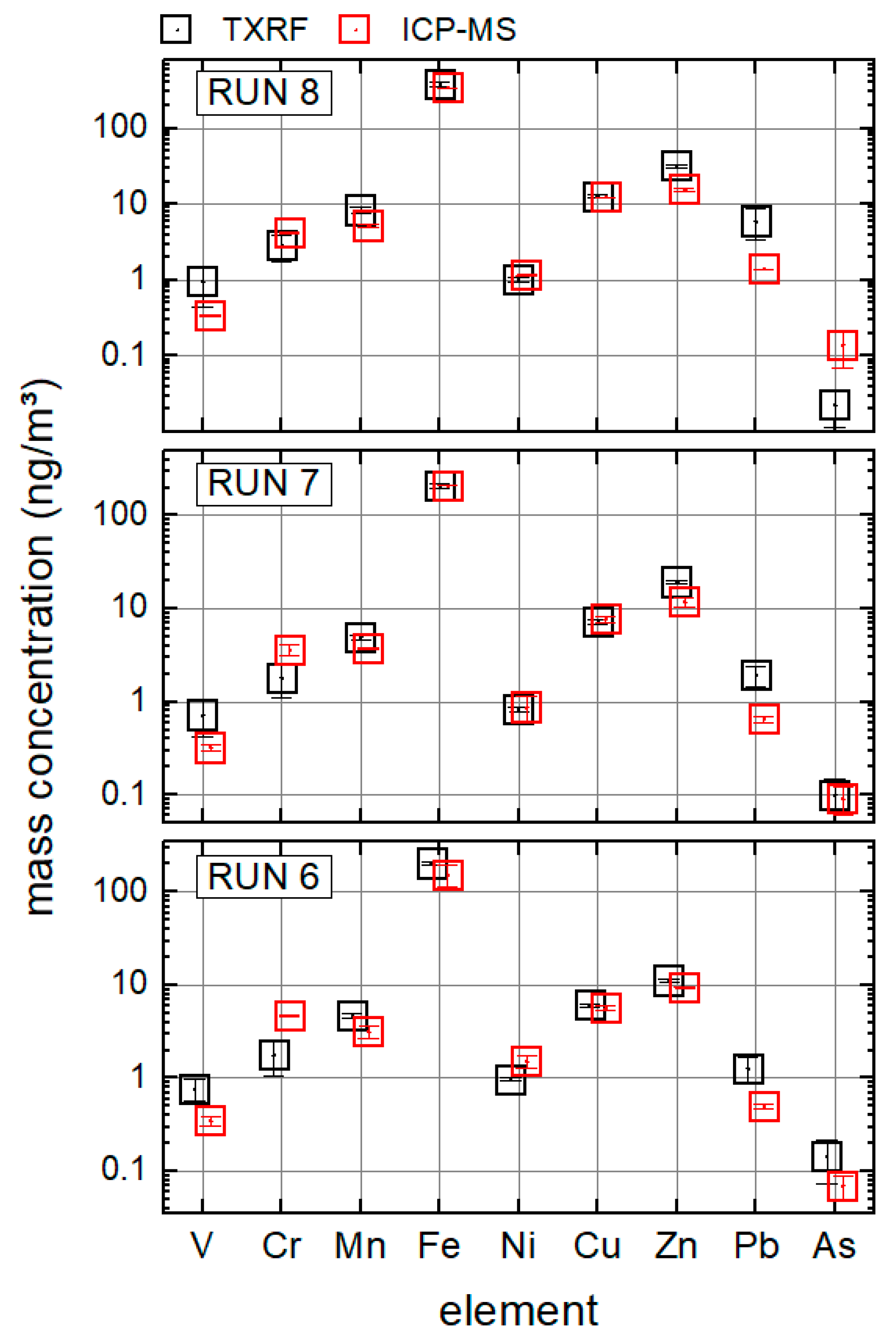
Figure 2 reveals the comparison of element mass concentrations in the PM
10 fraction of samples from the field campaign, quantified by ICP-MS and TXRF.
The overall agreement is satisfactory for the proof of principles; the mass concentration levels as determined by ICP-MS could be corroborated by TXRF over several orders of magnitude. ICP-MS- and TXRF-error bars do not always overlap; this is in all three runs the case for V and Pb. For a quantitative comparison the relative deviations between ICP-MS and TXRF were calculated as mean values over runs 6, 7, and 8 by the following equation:
where
x depicting the element and
the measured mass concentrations
Mean relative deviations (RD) around ±50% or even smaller were found for most of the detected elements, as listed in
Table 4. V and Pb are clearly outside this range.
3.3. Size Resolved Element Quantification
A quite valuable feature of cascade impactors is the size resolved chemical analysis of aerosol particles. The question arises of how good the comparability of the size distributions of elements between impactors of distinct design and a different number of stages (i.e., different size resolutions) can be. In line with the expected lognormal distribution, size distributions of atmospheric elemental mass concentrations are presented in normalized form as
dCM/
dlogdp in ng/m
3, calculated from the mass concentrations in each size bin determined by TXRF. Discrete values for the cascade impactor stages are plotted at the representative diameter of each size bin, which is the geometrical mean of the cut-off diameters for each stage and the corresponding upwind stage. For comparison, the May-type carriers have been analyzed at the EK stationary TXRF spectrometer. The carriers’ aerosol deposits, i.e., the stripes, were oriented perpendicular to the incident X-ray beam direction. The elemental mass per sample (i.e., the total elemental mass deposited in the entire carrier stripe of 20 mm length) was calculated for each size fraction considering the difference in total lengths of the stripes on the carriers and the total length of the impactor nozzles (50 mm) and the losses involved. Detection limits of 100 pg/m
3 for each impactor stage were reached using the model for transition metals in ambient aerosol particles [
29].
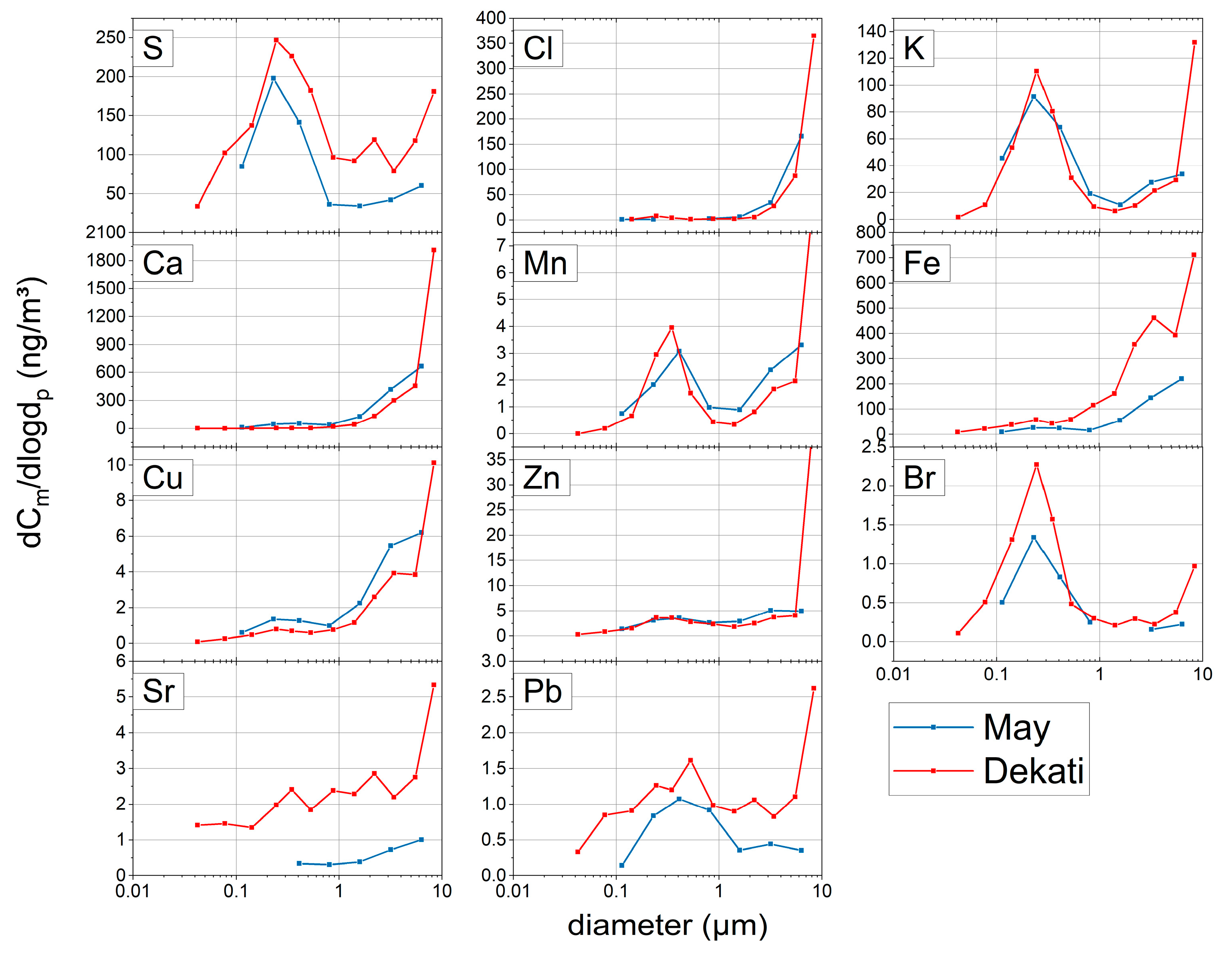
Figure 3 shows an example of fairly good correspondence of most element size distributions for the two impactor designs.
The size distribution from the Dekati impactor is a little bit more detailed due to the higher size resolution, and higher maxima in the largest size bin were obtained. This most likely occurred because the upper two stages of the May impactor were excluded from the analysis to optimally cover the PM10 size range; in effect, the geometric mean diameter of the largest size bin is 6.3 µm only while for the Dekati it is 8.4 µm. Differences, such as the huge coarse fraction contribution of Zn in the Dekati impactor data, and the mismatch of size distributions for Sr, Fe, and Pb, will need further investigations. Arsenic was—due to the problematic spectroscopic deconvolution of Pb and As contributions—not considered in this comparison. The proper quantification of As and Pb in TXRF spectra could not be fully solved within the scope of this project.
3.4. Results from Experiment 3
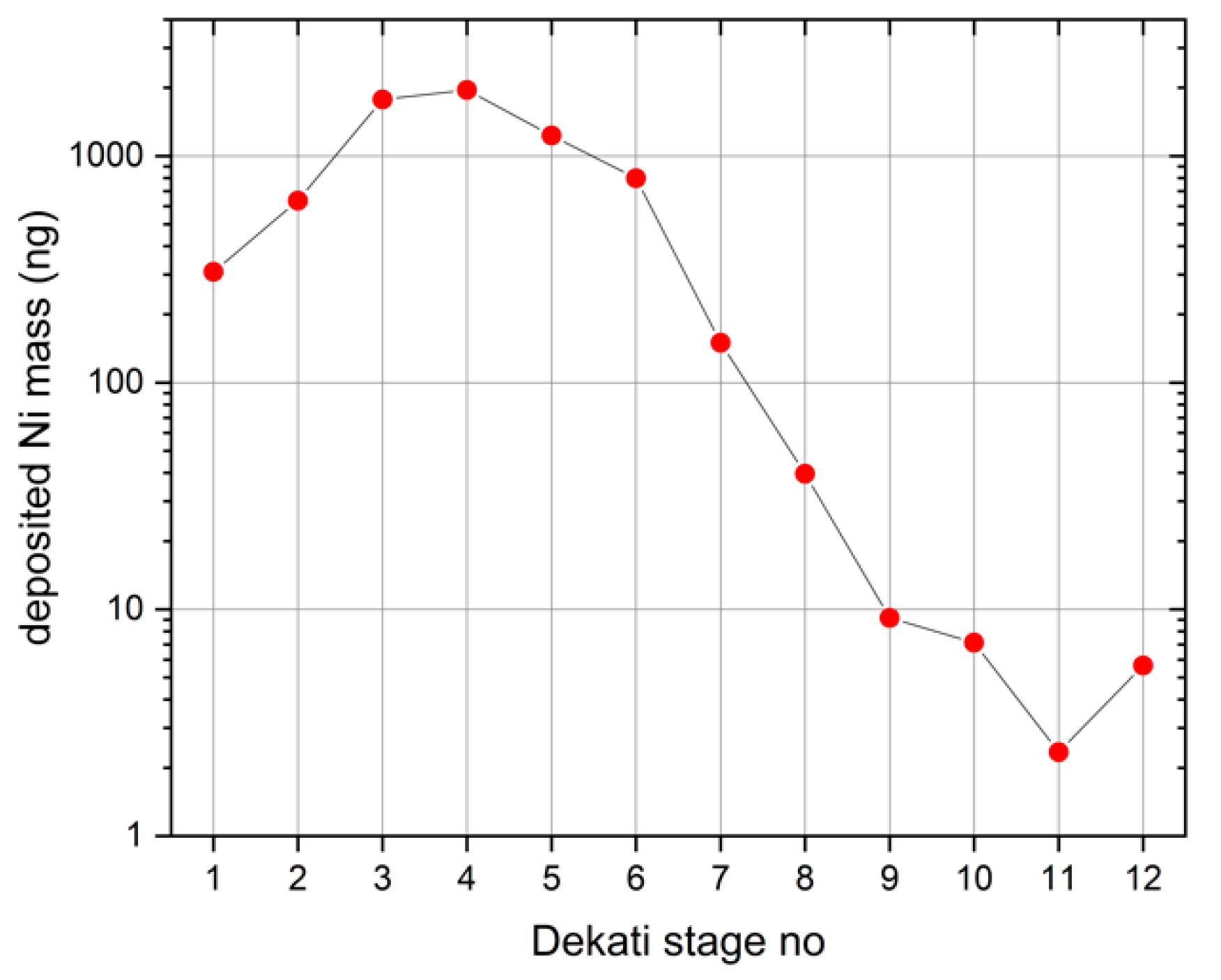
The S2 TXRF spectrometer used in the field campaign was calibrated against the elemental mass depositions as determined by a physically traceable, reference-free X-ray spectrometry (XRS) arrangement. In the first step, a nickel (Ni) test aerosol with broad size distribution was sampled onto a set of 12 acrylic discs carriers, which had been prepared by spiking in the center with an internal standard (50 ng Yttrium). The carriers were analyzed with the S2 spectrometer, and deposits of Ni on all stages in quantities between more than 1000 ng and several ng, well above the LLOD of the S2 spectrometer could be measured as shown in
Figure 4; the relative uncertainties are below two per mil.
The quantifications were based on the applied internal Y standard and using Equation (2).
where
is the determined mass of nickel on the carrier of impactor stage
k. and
describe the count rates of nickel and the internal Y standard and the tabulated relative sensitivities are given by
and
.
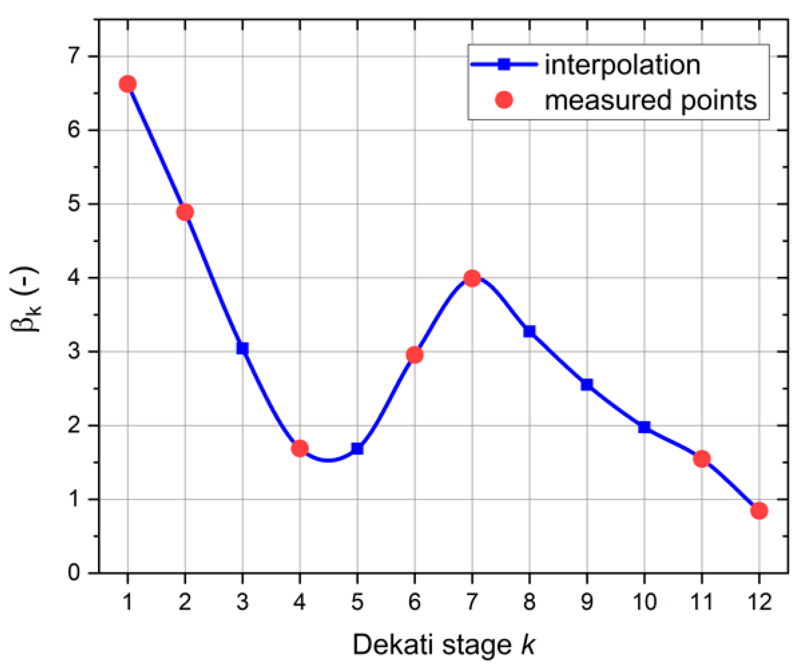
Finally, a selection (stages 1, 2, 4, 6, 7, 11, and 12) from the same set of carriers were remeasured with the above-described reference-free XRS methodology from PTB by complete lateral scanning of the carriers’ surfaces (as mapping is rather time-consuming, stages 5 and 8 to 10 could not be measured, due to limited beamtime at the PTB beamline at the BESSY II facility).
The stagewise comparison of both results enabled the quantification of the above discussed influences from the deposition patterns, such as radially varying deposition densities and lateral extensions, which may result in stage-dependent effects on the excitation, absorption, and detection of XRF radiation. The comparison resulted in stage-individual calibration factors,
, which were calculated by Equation (3):
where
depicts the masses of nickel on the carrier of impactor stage
k as measured by the reference method (lateral scanning).
The result is shown in
Figure 5 as an interpolated correction curve. With this set of calibration factors, all TXRF data from the field campaign have been corrected before comparison with the ICP-MS results.
5. Conclusions
The first on-site application of cascade impactors and mobile TXRF for the measurement of element concentrations in ambient aerosols revealed that operation of the impactors and manipulation of carriers, as well as TXRF spectroscopy, is technically workable under the conditions of field campaigns. The carrier loading sets upper limits with regards to the absolute particle mass concentration in the aerosol, sampling time, and sampling flow rates have to be selected to keep the sampled masses within the bounds of the TXRF spectroscopy. On the other hand, very short sampling intervals below 12 h are feasible, which observes the temporal variations in small element mass concentrations.
The method also gives insight into the size distribution of elements in an aerosol. This provides new, flexible options for the chemical analysis of ambient aerosol sources that can adapt quickly to changing atmospheric or indoor air conditions. It can be stated that the method has the potential to grow into a standard method for the chemical analysis of aerosols.
The concept of experimentally calibrating the S2 TXRF spectrometer was demonstrated to analyze aerosol cascade impactors samples using reference-free XRS and using a set of synthetic samples. This strategy proved its usefulness, although several deficiencies are still to be solved to increase the accuracy to an acceptable level. The obtained results can be seen as a successful proof of principles, which have already motivated continuing the research in the framework of a follow-up EMPIR project (AEROMET II [
46]). This project addresses inter alia one of the key challenges ahead: The calibration based on a robust and independent SI traceable reference method, which includes impactor designs, stage-individual corrections, and development of certified reference samples, as well as robust analysis algorithms.


 ,
, 


