
The Combined Effects of SST and the North Atlantic Subtropical High-Pressure System on the Atlantic Basin Tropical Cyclone Interannual Variability

 ,
,  ,
,  ,
,  and
and 
Abstract
:1. Introduction
2. Materials and Methods
2.1. Dataset
2.2. Methodology
Kernel Density Estimation
3. Results and Discussion
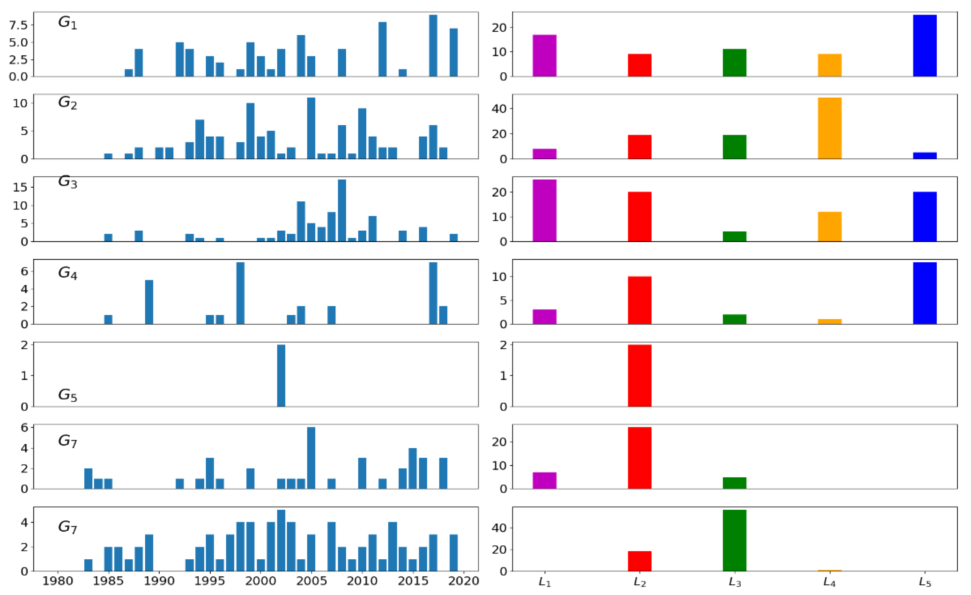
3.1. TC Genesis
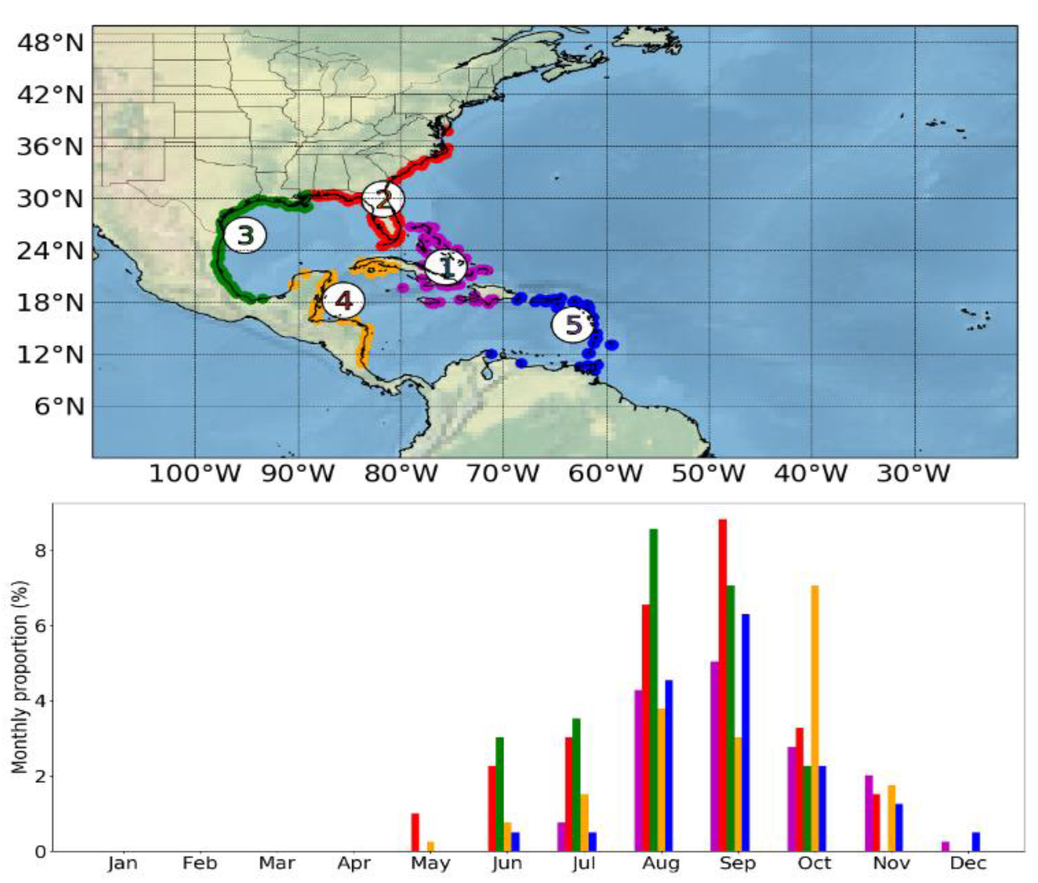
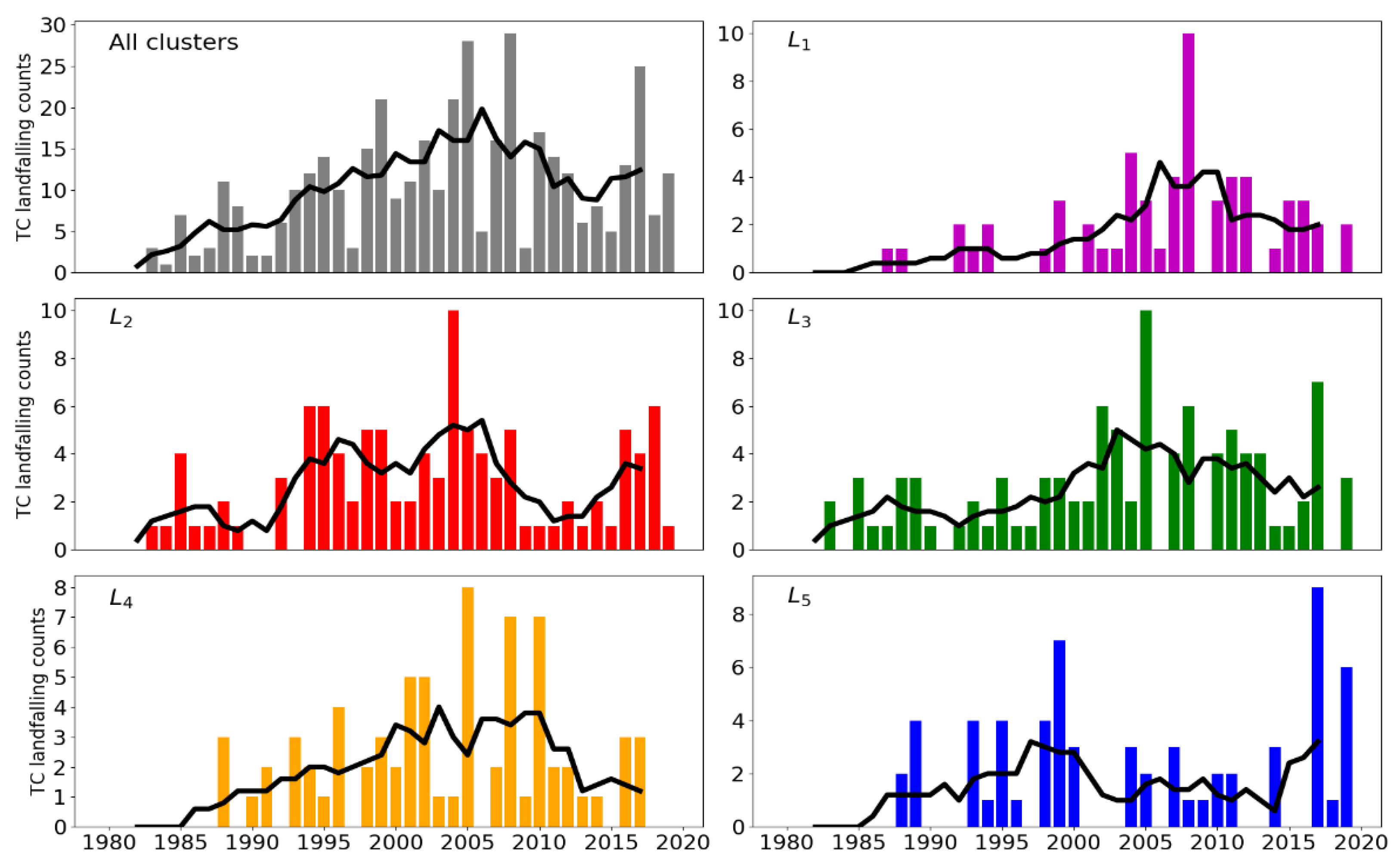
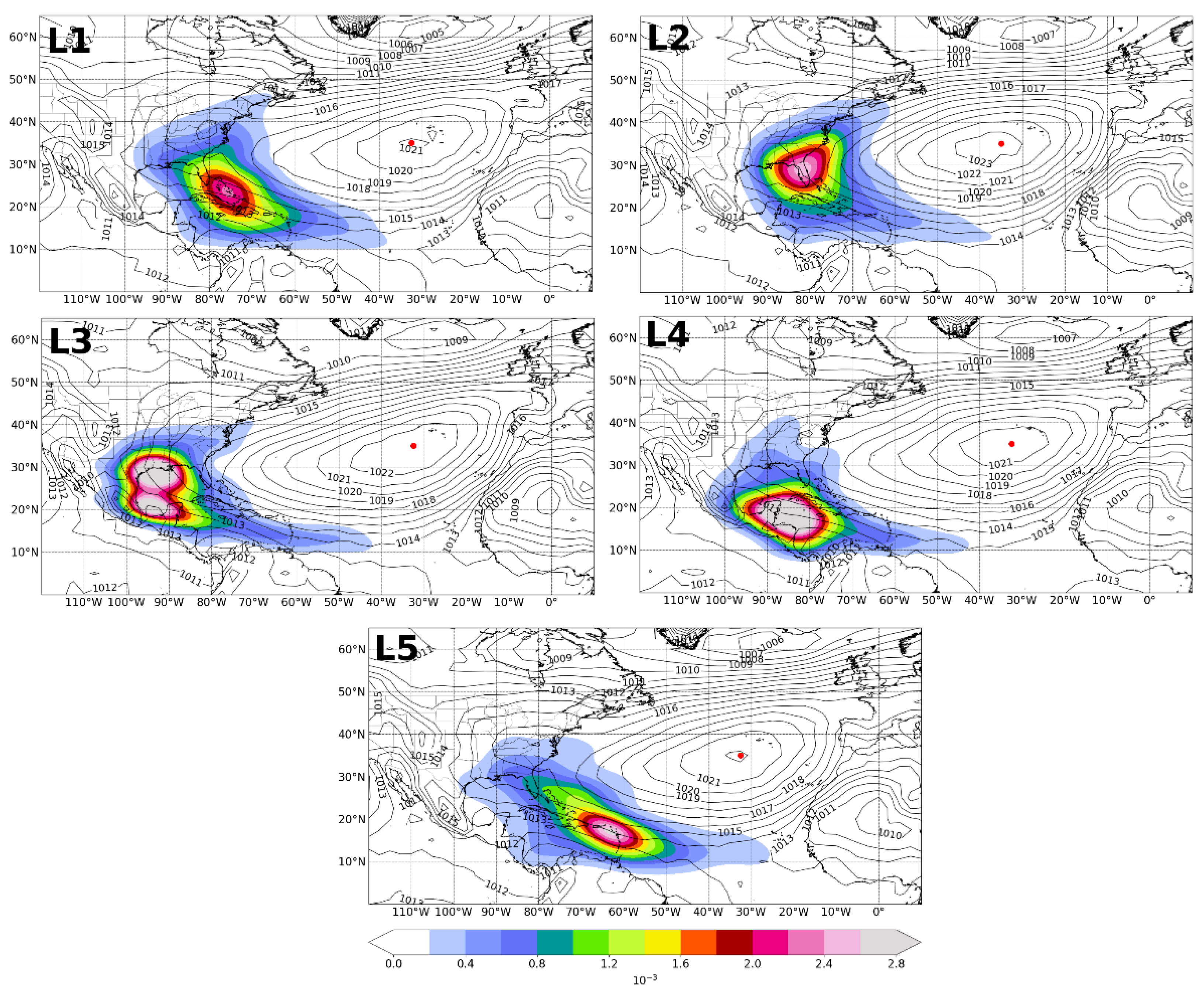
3.2. Landfall
4. Conclusions
Author Contributions
Funding
Acknowledgments
Conflicts of Interest
References
- Ankur, K.; Busireddy, N.K.R.; Osuri, K.K.; Niyogi, D. On the relationship between intensity changes and rainfall distribution in tropical cyclones over the North Indian Ocean. Int. J. Climatol. 2020, 40, 2015–2025. [Google Scholar] [CrossRef]
- Duan, H.; Chen, D.; Lie, J. The Impact of Global Warming on Hurricane Intensity. IOP Conf. Ser. Earth Environ. Sci. 2018, 199, 022045. [Google Scholar] [CrossRef]
- Goldenberg, S.B.; Landsea, C.W.; Mestas-Nuñez, A.M.; Gray, W.M. The Recent Increase in Atlantic Hurricane Activity: Causes and Implications. Science 2001, 293, 474–479. [Google Scholar] [CrossRef] [Green Version]
- Trenberth, K. Uncertainty in Hurricanes and Global Warming. Science 2005, 308, 1753–1754. [Google Scholar] [CrossRef] [Green Version]
- Frank, W.M.; Young, G.S. The interannual variability of tropical cyclones. Mon. Weather Rev. 2007, 135, 3587–3598. [Google Scholar] [CrossRef]
- Holland, G.; Bruyere, C.L. Recent intense hurricane response to global climate change. Clim. Dyn. 2014, 42, 617–627. [Google Scholar] [CrossRef] [Green Version]
- Kossin, J.; Emanuel, K.; Vecchi, G. The poleward migration of the location of tropical cyclone maximum intensity. Nature 2014, 509, 349–352. [Google Scholar] [CrossRef] [PubMed] [Green Version]
- Kossin, J.P.; Olander, T.L.; Knapp, K.R. Trend Analysis with a New Global Record of Tropical Cyclone Intensity. J. Clim. 2013, 26, 9960–9976. [Google Scholar] [CrossRef]
- Landsea, C.W.; Harper, B.A.; Hoarau, K.; Knaff, J.A. Can we detect trends in extreme tropical cyclones? Science 2006, 313, 452–454. [Google Scholar] [CrossRef] [PubMed] [Green Version]
- Vecchi, G.A.; Knutson, T.R. Estimating annual numbers of Atlantic hurricanes missing from the HURDAT database (1878–1965) using ship track density. J. Clim. 2011, 24. [Google Scholar] [CrossRef]
- Landsea, C.W.; Vecchi, G.A.; Bengtsson, L.; Knutson, T.R. Impact of duration thresholds on Atlantic tropical cyclone counts. J. Clim. 2010, 23, 2508–2519. [Google Scholar] [CrossRef]
- Vecchi, G.A.; Knutson, T.R. On Estimates of Historical North Atlantic Tropical Cyclone Activity. J. Clim. 2008, 21, 3580–3600. [Google Scholar] [CrossRef]
- Knutson, T.R.; McBride, J.L.; Chan, J.; Emanuel, K.; Holland, G.; Landsea, C.; Held, I.; Kossin, J.P.; Srivastava, A.K.; Sugi, M. Tropical cyclones and climate change. Nat. Geosci. 2010, 3, 157–163. [Google Scholar] [CrossRef] [Green Version]
- Palmen, E. On the formation and structure of tropical hurricanes. Geophysica 1948, 3, 26–38. [Google Scholar]
- Miller, B.I. On the maximum intensity of hurricanes. J. Atmos. Sci. 1958, 15, 184–195. [Google Scholar] [CrossRef] [Green Version]
- Riehl, H. Tropical Meteorology; McGraw-Hill: New York, NY, USA, 1954; 392p. [Google Scholar]
- Kaplan, J.; DeMaria, M. Large-Scale Characteristics of Rapidly Intensifying Tropical Cyclones in the North Atlantic Basin. Weather Forecast. 2003, 18, 1093–1108. [Google Scholar] [CrossRef] [Green Version]
- Trenberth, K.E.; Davis, C.A.; Fasullo, J. Water and energy budgets of hurricanes: Case studies of Ivan and Katrina. J. Geophys. Res. 2007, 112, D23106. [Google Scholar] [CrossRef]
- Shay, L.K.; Goni, G.J.; Black, P.G. Effects of a warm oceanic feature on Hurricane Opal. Mon. Weather Rev. 2000, 128, 1366–1383. [Google Scholar] [CrossRef]
- Goni, G.; Trinanes, J. Ocean thermal structure monitoring could aid in the intensity forecast of tropical cyclones. Eos. Trans. Am. Geophys. Union 2003, 84, 573–580. [Google Scholar] [CrossRef] [Green Version]
- Ma, Z.; Fei, J.; Liu, L.; Huang, X.; Cheng, X. Effects the cold core eddy on tropical cyclone intensity and structure under idealized air–sea interaction conditions. Mon. Weather Rev. 2013, 141, 1285–1303. [Google Scholar] [CrossRef]
- Trigo, R.M.; Gimeno, L. Observed Impacts on Planet Earth. In Weather Pattern Changes in Weather Mid-Latitudes the Tropics Pattern and Changes, Climate Change, 2nd ed.; Elsevier: Amsterdam, The Netherlands, 2016; Chapter 7; pp. 105–119. [Google Scholar]
- Sun, Y.; Zhong, Z.; Li, T.; Yijia, H.; Hu, Y.; Wan, H.; Chen, H.; Liao, Q.; Ma, C.; Li, Q. Impact of Ocean Warming on Tropical Cyclone Size and Its Destructiveness. Sci. Rep. 2017, 7, 8154. [Google Scholar] [CrossRef] [PubMed]
- Wu, L.; Wen, Z.; Huang, R. Tropical cyclones in a warming climate. Sci. China Earth Sci. 2020, 63, 456–458. [Google Scholar] [CrossRef]
- Santer, B.D.; Wigley, T.M.L.; Gleckler, P.J.; Bonfils, C.; Wehner, M.F.; AchutaRao, K.; Barnett, T.P.; Boyle, J.S.; Brüggemann, W.; Fiorino, M.; et al. Forced and unforced ocean temperature changes in Atlantic and Pacific tropical cyclogenesis regions. Proc. Natl. Acad. Sci. USA 2006, 103, 13905–13910. [Google Scholar] [CrossRef] [Green Version]
- Knutson, T.R.; Delworth, T.L.; Dixon, K.W.; Held, I.M.; Lu, J.; Ramaswamy, V.; Schwarzkopf, M.D.; Stenchikov, G.; Stouffer, R.J. Assessment of Twentieth-Century Regional Surface Temperature Trends Using the GFDL CM2 Coupled Models. J. Clim. 2006, 19, 1624–1651. [Google Scholar] [CrossRef] [Green Version]
- Xie, L. The effect of Atlantic sea surface temperature dipole mode on hurricanes: Implications for the 2004 Atlantic hurricane season. Geophys. Res. Lett. 2005, 32, L03701. [Google Scholar] [CrossRef] [Green Version]
- Xie, K.; Liu, B. An ENSO-Forecast Independent Statistical Model for the Prediction of Annual Atlantic Tropical Cyclone Frequency in April. Adv. Meteorol. 2014, 2014, 1–11. [Google Scholar] [CrossRef] [Green Version]
- Xu, J.; Wang, Y.; Tan, Z. The Relationship between Sea Surface Temperature and Maximum Intensification Rate of Tropical Cyclones in the North Atlantic. J. Atmos. Sci. 2016, 73, 4979–4988. [Google Scholar] [CrossRef]
- Foltz, G.R.; Balaguru, K.; Hagos, S. Interbasin Differences in the Relationship between SST and Tropical Cyclone Intensification. Mon. Weather Rev. 2018, 146, 853–870. [Google Scholar] [CrossRef]
- Webster, P.J.; Holland, G.J.; Curry, J.A.; Chang, H.R. Changes in Tropical Cyclone Number, Duration, and Intensity in a Warming Environment. Science 2005, 309, 1844–1846. [Google Scholar] [CrossRef] [Green Version]
- Zhang, Y.; Zhang, Z.; Chen, D.; Qiu, B.; Wanget, W. Strengthening of the Kuroshio current by intensifying tropical cyclones. Science 2020, 368, 988. [Google Scholar] [CrossRef]
- Emanuel, K. Increasing destructiveness of tropical cyclones over the past 30 years. Nature 2005, 436, 686–688. [Google Scholar] [CrossRef] [PubMed]
- Deser, C.; Alexander, M.A.; Xie, S.-P.; Phillips, A.S. Sea surface temperature variability: Patterns and mechanisms. Annu. Rev. Mar. Sci. 2010, 2, 115–143. [Google Scholar] [CrossRef] [PubMed] [Green Version]
- Kossin, J.P.; Camargo, S.J.; Sitkowski, M. Climate modulation of North Atlantic hurricane tracks. J. Clim. 2010, 23, 3057–3076. [Google Scholar] [CrossRef]
- Colbert, A.; Soden, B. Climatological variations in North Atlantic tropical cyclone tracks. J. Clim. 2012, 25, 657–673. [Google Scholar] [CrossRef]
- Fudeyasu, H.; Hirose, S.; Yoshioka, H.; Kumazawa, R.; Yamasaki, S. A Global View of the Landfall Characteristics of Tropical Cyclones. Trop Cyclone Res. Rev. 2014, 3, 178–192. [Google Scholar] [CrossRef]
- Dailey, P.S.; Zuba, G.; Ljung, G.; Dima, J.M.; Guin, J. On the Relationship between North Atlantic Sea Surface Temperatures and U.S. Hurricane Landfall Risk. J. Appl. Meteorol. Climatol. 2009, 48, 111–129. [Google Scholar] [CrossRef]
- Elsner, J.B.; Bossak, H.; Niu, H.F. Secular changes to the ENSO-U.S. hurricane relationship. Geophys. Res. Lett. 2012, 28, 4123–4126. [Google Scholar] [CrossRef]
- Li, W.; Li, L.; Ting, M.; Liu, Y. Intensification of Northern Hemisphere subtropical highs in a warming climate. Nat. Geosci. 2012, 5, 830–834. [Google Scholar] [CrossRef]
- Jarvinen, B.R.; Neumann, C.J.; Davis, M.A.S. A tropical cyclone data tape for the North Atlantic Basin, 1886–1983: Contents, limitations, and uses. NOAA Technical Memorandum 1984, NWS NHC 22, Coral Gables, FL, 24 p. Available online: http://www.nhc.noaa.gov/pdf/NWS-NHC-1988-22.pdf (accessed on 15 November 2020).
- Landsea, C.W.; Franklin, J.L. Atlantic Hurricane Database Uncertainty and Presentation of a New Database Format. Mon. Weather Rev. 2013, 141, 3576–3592. [Google Scholar] [CrossRef]
- Atlantic Hurricane Database (HURDAT2). Available online: https://www.nhc.noaa.gov/data/hurdat/hurdat2-1851-2019-052520.txt (accessed on 2 September 2020).
- Dvorak, V.F. Tropical cyclone intensity analysis and forecasting from satellite imagery. Mon. Wea. Rev. 1975, 103, 420–430. [Google Scholar] [CrossRef]
- Dvorak, V.F. Tropical Cyclone Intensity Analysis Using Satellite Data; NOAA Technical Report; NESDIS: Silver Spring, MD, USA, 1984; Volume 11, p. 47. [Google Scholar]
- Bhatia, K.T.; Vecchi, G.A.; Knutson, T.R.; Murakami, H.; Kossin, J.; Dixon, K.W.; Whitlock, C.E. Recent increases in tropical cyclone intensification rates. Nat. Commun. 2019, 10, 635. [Google Scholar] [CrossRef]
- Chang, E.K.M.; Guo, Y. Is the number of North Atlantic tropical cyclones significantly underestimated prior to the availability of satellite observations? Geophys. Res. Lett. 2007, 34, L14801. [Google Scholar] [CrossRef] [Green Version]
- Kang, N.; Elsner, J.B. Consensus on Climate Trends in Western North Pacific Tropical Cyclones. J. Clim. 2012, 25, 7564–7573. [Google Scholar] [CrossRef] [Green Version]
- Centennial Time Scale (COBE SST2) Dataset. Available online: https://psl.noaa.gov/data/gridded/data.cobe2.html (accessed on 18 September 2020).
- Hirahara, S.; Ishii, M.; Fukuda, Y. Centennial-scale sea surface temperature analysis and its uncertainty. J. Clim. 2014, 27, 57–75. [Google Scholar] [CrossRef]
- Kalnay, E.; Kanamitsu, M.; Kistler, R.; Collins, W.; Deaven, D.; Gandin, L.; Iredell, M.; Saha, S.; White, G.; Woollen, J.; et al. The NCEP/NCAR 40-Year Reanalysis Project. Bull. Am. Meteorol. Soc. 1996, 77, 437–472. [Google Scholar] [CrossRef] [Green Version]
- Knapp, K.R.; Kruk, M.C.; Levinson, D.H.; Diamond, H.J.; Neumann, C.J. The International Best Track Archive for Climate Stewardship (IBTrACS): Unifying tropical cyclone best track data. Bull. Am. Meteorol. Soc. 2010, 91, 363–376. [Google Scholar] [CrossRef]
- Corporal-Lodangco, I.L.; Richman, M.B.; Leslie, L.M.; Lamb, P.J. Cluster Analysis of North Atlantic Tropical Cyclones. Procedia Comput. Sci. 2014, 36, 293–300. [Google Scholar] [CrossRef] [Green Version]
- Reboita, M.S.; Ambrizzi, T.; Silva, B.A.; Pinheiro, R.F.; da Rocha, R.P. The South Atlantic Subtropical Anticyclone: Present and Future Climate. Front. Earth Sci. 2019, 7, 8. [Google Scholar] [CrossRef] [Green Version]
- Degola, T.S.D. Impacts and Variability of the South Atlantic Subtropical Anticyclone on Brazil in the Present Climate and in Future Scenarios. Master’s Thesis, University of São Paulo, São Paulo, Brazil, 2013. [Google Scholar]
- Lambert, S.J. A cyclone climatology of the Canadian centre general circulation model. J. Clim. 1988, 1, 109–115. [Google Scholar] [CrossRef] [Green Version]
- Murray, R.J.; Simmonds, I. A numerical scheme for tracking cyclone centres from digital data. Austr. Meteorol. Mag. 1991, 39, 155–166. [Google Scholar]
- Sinclair, M.R. A diagnostic model for estimating orographic precipitation. J. Appl. Meteorol. Climatol. 1994, 33, 1163–1175. [Google Scholar] [CrossRef] [Green Version]
- Sugahara, S. Annual Variation of the Frequency of Cyclones in the South Atlantic Ocean. In Proceedings of the XI Brazilian Congress of Meteorology, Rio de Janeiro, Brazil, 16–20 June 2000. [Google Scholar]
- Bretherton, C.S.; Widmann, M.; Dymnikov, V.P.; Wallace, J.M.; Bladé, I. The effective number of spatial degrees of freedom of a time-varying field. J. Clim. 1999, 12, 1990–2009. [Google Scholar] [CrossRef]
- Kim, T.K. T test as a parametric statistic. Korean J. Anesthesiol. 2015, 68, 540. [Google Scholar] [CrossRef] [PubMed] [Green Version]
- Safi, S.K.; Saif, E.A.A. Using GLS to Generate Forecasts in Regression Models with Auto-correlated Disturbances with simulation and Palestinian Market Index Data. Am. J. Theor. Appl. Stat. 2014, 3, 6–17. [Google Scholar] [CrossRef] [Green Version]
- Davidson, R.; MacKinnon, J.G. Econometric Theory and Methods; Oxford University Press: Oxford, UK, 2004. [Google Scholar]
- Wahiduzzaman, M.; Yeasmin, A. A kernel density estimation approach of North Indian Ocean tropical cyclone formation and the association with convective available potential energy and equivalent potential temperature. Meteorol. Atmos. Phys. 2020, 132, 603–612. [Google Scholar] [CrossRef]
- Loader, C.R. Bandwidth Selection: Classical or Plug-In? Ann. Stat. 1999, 27, 415–438. [Google Scholar] [CrossRef]
- Gray, W.M. Global view of the origin of tropical disturbances and storms. Mon. Weather Rev. 1968, 96, 669–700. [Google Scholar] [CrossRef]


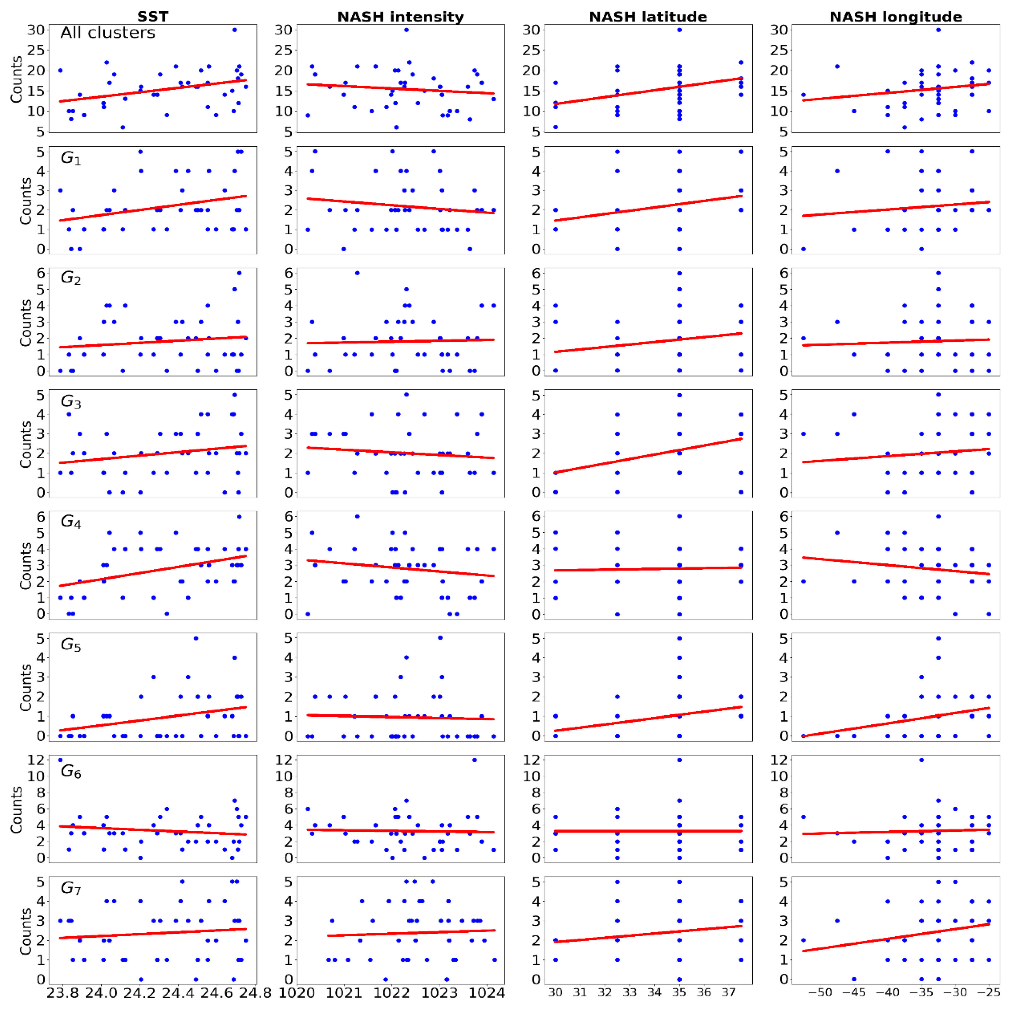
| All Clusters | G1 | G2 | G3 | G4 | G5 | G6 | G7 | |
|---|---|---|---|---|---|---|---|---|
| SST | 0.35 | 0.36 | 0.13 | 0.21 | 0.39 | 0.30 | −0.14 | −0.004 |
| NASH intensity | −0.12 | −0.15 | 0.04 | −0.10 | −0.17 | −0.04 | −0.03 | 0.07 |
| NASH latitude | 0.36 | 0.26 | 0.20 | 0.36 | 0.03 | 0.26 | 0.01 | 0.16 |
| NASH longitude | 0.18 | 0.11 | 0.05 | 0.10 | −0.14 | 0.25 | 0.05 | 0.21 |
| All Clusters | G1 | G2 | G3 | G4 | G5 | G6 | G7 | ||
|---|---|---|---|---|---|---|---|---|---|
| R2 | 0.227 | 0.151 | 0.055 | 0.186 | 0.191 | 0.153 | 0.036 | 0.05 | |
| Intercept | Estimated | 706.27 | 205.67 | −78.67 | 231.85 | −24.29 | 62.03 | 328.4 | −18.75 |
| Std error | 918.01 | 267.66 | 324.98 | 254.97 | 295.13 | 0.80 | 473.2 | 301.95 | |
| p value | 0.45 | 0.447 | 0.810 | 0.369 | 0.935 | 0.250 | 0.492 | 0.95 | |
| SST | Coefficient | 3.71 | 0.905 | 0.55 | 0.597 | 1.93 | 0.96 | −1.372 | 0.35 |
| Std error | 2.53 | 0.738 | 0.89 | 0.53 | 0.814 | 0.683 | 1.305 | 0.83 | |
| p value | 0.15 | 0.228 | 0.615 | 0.70 | 0.023 | 0.168 | 0.301 | 0.68 | |
| NASH intensity | Coefficient | −0.79 | −0.23 | 0.059 | −0.24 | −0.023 | −0.08 | −0.285 | 0.013 |
| Std error | 0.87 | 0.256 | 0.310 | 0.243 | 0.282 | 0.237 | 0.452 | 0.28 | |
| p value | 0.37 | 0.382 | 0.85 | 0.324 | 0.93 | 0.723 | 0.533 | 0.96 | |
| NASH latitude | Coefficient | 0.82 | 0.171 | 0.165 | 0.27 | 0.060 | 0.09 | 0.018 | 0.034 |
| Std error | 0.43 | 0.125 | 0.152 | 0.119 | 0.138 | 0.116 | 0.221 | 0.141 | |
| p value | 0.065 | 0.18 | 0.28 | 0.026 | 0.665 | 0.436 | 0.935 | 0.809 | |
| NASH longitude | Coefficient | 0.008 | −0.001 | −0.025 | −0.018 | −0.059 | 0.033 | 0.036 | 0.041 |
| Std error | 0.148 | 0.043 | 0.052 | 0.041 | 0.048 | 0.040 | 0.076 | 0.049 | |
| p value | 0.960 | 0.976 | 0.64 | 0.65 | 0.23 | 0.410 | 0.638 | 0.404 |
| All Clusters | L1 | L2 | L3 | L4 | L5 | |
|---|---|---|---|---|---|---|
| SST | 0.52 | 0.44 | 0.30 | 0.46 | 0.33 | 0.30 |
| NASH intensity | −0.04 | −0.05 | −0.15 | −0.08 | 0.17 | −0.03 |
| NASH latitude | 0.42 | 0.34 | 0.26 | 0.30 | 0.38 | 0.25 |
| NASH longitude | 0.29 | 0.40 | 0.05 | 0.21 | 0.22 | 0.18 |
| All Clusters | L1 | L2 | L3 | L4 | L5 | ||
|---|---|---|---|---|---|---|---|
| R2 | 0.387 | 0.334 | 0.177 | 0.264 | 0.241 | 0.118 | |
| Intercept | Estimated | −85.9351 | 125.97 | 292.02 | 47.2604 | −529.73 | −21.45 |
| Std error | 1286.201 | 354.64 | 445.55 | 417.389 | 404.789 | 447.52 | |
| p value | 0.947 | 0.725 | 0.516 | 0.910 | 0.199 | 0.962 | |
| SST | Coefficient | 11.061 | 2.3545 | 1.605 | 2.9128 | 2.2941 | 1.8939 |
| Std error | 3.548 | 0.978 | 1.222 | 1.151 | 1.117 | 1.235 | |
| p value | 0.004 | 0.022 | 0.200 | 0.016 | 0.047 | 0.134 | |
| NASH intensity | Coefficient | −0.2033 | −0.178 | −0.336 | −0.1195 | 0.4554 | −0.0251 |
| Std error | 1.228 | 0.339 | 0.425 | 0.399 | 0.386 | 0.427 | |
| p value | 0.869 | 0.603 | 0.435 | 0.766 | 0.247 | 0.953 | |
| NASH latitude | Coefficient | 1.109 | 0.1120 | 0.382 | 0.2169 | 0.2869 | 0.1119 |
| Std error | 0.601 | 0.166 | 0.208 | 0.195 | 0.189 | 0.209 | |
| p value | 0.073 | 0.504 | 0.075 | 0.274 | 0.139 | 0.596 | |
| NASH longitude | Coefficient | 0.1063 | 0.111 | −0.064 | 0.0296 | −0.0069 | 0.0363 |
| Std error | 0.208 | 0.057 | 0.072 | 0.067 | 0.065 | 0.072 | |
| p value | 0.612 | 0.061 | 0.383 | 0.662 | 0.917 | 0.618 |
| All Clusters | L1 | L2 | L3 | L4 | L5 | |
|---|---|---|---|---|---|---|
| Year | 2008 | 2008 | 2004 | 2005 | 2005 | 2017 |
| Landfall counts | 29 | 10 | 10 | 10 | 8 | 9 |
Publisher’s Note: MDPI stays neutral with regard to jurisdictional claims in published maps and institutional affiliations. |
© 2021 by the authors. Licensee MDPI, Basel, Switzerland. This article is an open access article distributed under the terms and conditions of the Creative Commons Attribution (CC BY) license (http://creativecommons.org/licenses/by/4.0/).
Share and Cite
Pérez-Alarcón, A.; Fernández-Alvarez, J.C.; Sorí, R.; Nieto, R.; Gimeno, L. The Combined Effects of SST and the North Atlantic Subtropical High-Pressure System on the Atlantic Basin Tropical Cyclone Interannual Variability. Atmosphere 2021, 12, 329. https://0-doi-org.brum.beds.ac.uk/10.3390/atmos12030329
Pérez-Alarcón A, Fernández-Alvarez JC, Sorí R, Nieto R, Gimeno L. The Combined Effects of SST and the North Atlantic Subtropical High-Pressure System on the Atlantic Basin Tropical Cyclone Interannual Variability. Atmosphere. 2021; 12(3):329. https://0-doi-org.brum.beds.ac.uk/10.3390/atmos12030329
Chicago/Turabian StylePérez-Alarcón, Albenis, José C. Fernández-Alvarez, Rogert Sorí, Raquel Nieto, and Luis Gimeno. 2021. "The Combined Effects of SST and the North Atlantic Subtropical High-Pressure System on the Atlantic Basin Tropical Cyclone Interannual Variability" Atmosphere 12, no. 3: 329. https://0-doi-org.brum.beds.ac.uk/10.3390/atmos12030329