Characteristics of Historical Precipitation in High Mountain Asia Based on a 15-Year High Resolution Dynamical Downscaling

Abstract

The mountains of High Mountain Asia serve as an important source of water for roughly one billion people living downstream. This research uses 15 years of dynamically downscaled precipitation produced by the Weather Research and Forecasting (WRF) model to delineate contrasts in precipitation characteristics and events between regions dominated by the Indian Summer Monsoon (ISM) versus westerly disturbances during the cool season (December to March). Cluster analysis reveals a more complex spatial pattern than indicated by some previous studies and illustrates the increasing importance of westerly disturbances at higher elevations. Although prior research suggests that a small number of westerly disturbances dominate precipitation in the western Himalaya and Karakoram, the WRF-downscaled precipitation is less dominated by infrequent large events. Integrated vapor transport (IVT) and precipitation are tightly coupled in both regions during the cool season, with precipitation maximizing for IVT from the south-southwest over the Karakoram and southeast-southwest over the western Himalaya. During the ISM, Karakoram precipitation is not strongly related to IVT direction, whereas over the western Himalaya, primary and secondary precipitation maxima occur for flow from the west-southwest and northwest, respectively. These differences in the drivers and timing of precipitation have implications for hydrology, glacier mass balance, snow accumulation, and their sensitivity to climate variability and change.

1. Introduction

The mountains of High Mountain Asia (HMA) provide essential freshwater resources for over 1 billion people living downstream [1,2]. Mountain precipitation, much of which is stored as glaciers and seasonal snowpack and released through melting, is an important contributor to the flow of the largest rivers in this region [3,4,5]. Despite the importance of precipitation in HMA as a water resource, the complex terrain of HMA, combined with the sparse distribution of weather stations and significant contribution of snow-type precipitation at upper elevations, makes precipitation characterization in this region very challenging [6,7,8,9].

A long history of literature identifies two primary spatiotemporal patterns of precipitation in the region with precipitation in the eastern Himalaya dominated by the Indian Summer Monsoon (ISM, May–October) and precipitation in the Karakoram and western Himalaya dominated by cool-season cyclones known as westerly disturbances (WDs), e.g., [10,11,12,13]. While these patterns are well known, their spatial pattern in relation to the complex topography of the region is less well understood [14,15]. This is in part because many gridded precipitation datasets over HMA inadequately resolve the spatial distribution of precipitation in higher-elevation regions, and/or suffer from limited in situ observations and satellite precipitation estimate errors [16,17,18]. For example, Cannon et al. [19] studied the variability of WDs over the Himalayas with a 0.25° resolution dataset. The results show distinct differences in the spatiotemporal characteristics of WDs in the western Himalayas and Karakoram region, as compared to the central Himalayas. However, at such a coarse resolution, the data does not fully capture fine-scale spatial variations in precipitation or orographic effects that may be important in these regions. Lang et al. [20] used an observation network to characterize wintertime snowfall within the Marsyandi River basin in the Central Himalayas. While the in situ dataset allows for a finer-scale analysis than that of coarse-gridded products, the results may not be representative of the broader Himalayan range. Both these studies suggest a few large WDs produce a large fraction of annual precipitation in the Indus headwaters of northwest India and northern Pakistan, but further analysis is needed to fill spatial-temporal gaps in our understanding of these extreme events.

Recent work utilizing higher resolution products has significantly advanced our understanding of precipitation and its distribution within HMA. For example, Bookhagen and Burbank [21] leveraged 5-km resolution data from the Tropical Rainfall Measurement Mission (TRMM) and in situ measurements to analyze spatiotemporal patterns of precipitation in the Himalaya and found that topography is a dominant factor in precipitation, with topographic relief playing an important role. When evaluating the distribution of precipitation, studies utilizing higher resolution products have also increased our understanding of the spatial-temporal transition between WD and ISM dominance [22,23], illustrating these transitions have more complex relationships with topography than evident in coarser-resolution products. For instance, a strong correlation between atmospheric water transport and cool-season WDs was found over the western portion of the Himalayas but not over the Tibetan Plateau [23], a pattern not evident in coarser-resolution products.

While higher resolution products inherently provide greater spatial detail, they also tend to better represent precipitation in complex terrain. Maussion et al. [22] described overall improvements in precipitation accuracy when moving from 30-km to 10-km grid spacing for the High Asia Refined analysis (HAR), although the precipitation maxima were slightly underestimated. Pritchard et al. [24] found that the 10-km HAR product provided a good representation of precipitation and agreement with the majority of precipitation stations, though they noted discrepancies in narrow mountain valleys where the terrain was not captured at that model resolution, resulting in overestimated precipitation. The HAR version 2 (HARv2) is now available and provides a larger 10-km domain and improved spatial distribution of seasonal mean precipitation [25]. In an intercomparison of gridded precipitation datasets over the central Himalaya and southwestern Tibetan Plateau from May to September 2017, Hamm et al. [26] found that precipitation produced by the HARv2 and a version of the HARv2 run with 2-km grid spacing (HARv2 2 km) produced a better match compared to ground-based precipitation observations than other gridded datasets. The HARv2 2-km output exhibited a slight improvement relative to observational data, including improved daily precipitation statistics due in part to the explicit rather than parameterized convection. In simulations of two multi-day precipitation events, Bonekamp et al. [27] found increased accuracy in the spatial distribution of precipitation with grid spacings as small as 500 m, but also identified significant overestimations of orographic precipitation. While precipitation accuracy depends on numerous factors, such as model parameterizations, these studies do suggest a general trend towards greater precipitation accuracy with higher spatial resolution. As computational approaches, resources, and technology continue to improve, higher-resolution products become increasingly possible and available. This provides the opportunity to continue to advance our understanding of the spatial and temporal patterns in precipitation and precipitation dynamics in complex terrain.

Differences in the drivers and timing of precipitation have implications for hydrology, freshwater resources, glacier mass balance, snow accumulation, and their sensitivity to climate variability and change. Runoff from mountain precipitation contributes to streamflow critical for downstream inhabitants in lower-elevation regions, and the melting of glaciers and seasonal snow can act as a buffer during times of low precipitation [2,4,28,29]. This effect is especially pronounced in the Indus River basin of western India and Pakistan where lowland precipitation is limited, but snow and glaciers provide a major source of water to people living within and downstream of the mountain systems [4]. As a result, changes in climate could have pronounced effects on those living in the Indus watershed, as their water supply is more vulnerable than their neighbors who receive more precipitation from the ISM [4,29]. More broadly, Immerzeel et al. [2] highlight the Indus watershed as one of the most important and vulnerable “water towers” globally. Thus, it is critical to advance our understanding of the complex spatial-temporal relationships between precipitation timing, frequency, and magnitude with topography in this region.

This work aims to advance understanding of the spatiotemporal patterns of precipitation, centered on the Indus River basin, using 15 years of dynamically downscaled precipitation from a regional climate simulation with 4-km horizontal resolution and hourly temporal output, centered on the Indus basin. We leverage this product to build on previous work to further assess the spatial complexities in orographic precipitation in the region. Specifically, we examine the spatiotemporal distribution of precipitation across the region, the contribution of large precipitation events to annual precipitation, and how those precipitation statistics vary with topography. We then analyze the role of atmospheric water vapor transport in precipitation across the region, and how this role varies seasonally, spatially, and between large precipitation events.

2. Methods

2.1. Dynamical Downscaling

We use dynamically downscaled precipitation from the WRF regional climate simulation described and evaluated by Dars et al. [30] to examine the precipitation climate of HMA. This simulation uses the Advanced Research WRF (hereafter WRF) version 3.8.1 with lateral boundary and initial atmospheric and land-surface conditions provided by the Climate Forecast System Reanalysis [31,32] for the period from 2000–2015. We discard the first year (i.e., 2000) for spin-up and focus our analysis on the 15-year period from 2001–2015. The WRF was configured with three nested domains with 36-, 12-, and 4-km grid spacing (Figure 1; see [30] for WRF-model terrain). Ikeda et al. [33] showed that regional climate simulations with <6-km grid spacing exhibit significant improvements in precipitation fidelity in Colorado. The resolution of domain 3 was selected to better represent precipitation processes, patterns, and variability in the complex terrain of HMA, within the context of the selected parameterizations.

Studies that have sought to identify optimal model parameterizations to reduce model uncertainties have often focused on smaller time windows to allow for more detailed evaluation, tested different parameterization schemes, or added nested domains to increase resolution. These studies suggest there is not an optimal set of parameters for simulating all climate variables, and that the optimal parameters differ based on the goals of the analysis [25,34]. Based on initial benchmarking (see [30] for details), the final model configuration used here includes the Noah-MP land-surface [35], YSU boundary layer [36], Thompson cloud microphysics [37], RRTM longwave radiation [38], Dudhia shortwave radiation [39], revised MM5 surface layer, and Kain-Fritsch cumulus [40] parameterizations, the latter applied only on the 36- and 12-km outer domains so that the 4-km domain is convection-permitting. All three domains had 38 vertical levels. For reference, a summary of the modeling setup outlined in detail in Dars et al. [30] is presented in

Table 1. Model setup.

A. Physical Parameterization Schemes
Land surface model (LSM)	Noah multi-parameterization (Noah-MP) [35]
Planetary boundary layer (PBL)	Yonsei University (YSU) scheme [36]
Microphysics	Thompson microphysics scheme [37]
Longwave radiation	Rapid radiative transfer model (RRTM) [38]
Shortwave radiation	Dudhia scheme [39]
Land surface	Revised MM5 scheme [39]
Cumulus parameterization	Kain-Fritch scheme in d01 and d02 only [40]
B. Grids and Nesting Strategy
Nesting	3 nested domains (d01, d02, d03) two-way coupled
Horizontal grid spacing	36 km, 12 km, and 4 km
Map projection	Lambert conformal
Number of vertical layers	38
Center point of domains	30.75 °N, 76.00 °E
Timestep Domains size (X × Y)	120 s in d01, 40 s in d02 and 13.3 s in d03 Outer domain (d01) 146 × 115 Middle domain (d02) 271 × 220 Inner domain (d03) 526 × 403

.

The WRF simulation has been validated against temperature and precipitation data from twenty-three stations as well as precipitation data from TRMM [30]. The analysis of precipitation from 36-km, 12-km, and 4-km domains presented in Dars et al. [30] indicated a general reduction in the model bias following the model resolution increase. The innermost 4-km domain produced significantly reduced annual precipitation bias as well as seasonal bias compared to the 36- and 12-km domains. The 4-km domain still slightly overestimated annual precipitation (23% higher than the station data and 15% higher than TRMM), and a similar positive bias was also evident in the seasonal data for autumn (23% and 12%, respectively). In winter and spring, the positive model bias with respect to the station data was higher, 39% and 38%, respectively. During the summer, the innermost domain exhibited a slightly negative bias (−10% compared to the station data), which was higher than the 12-km domain d02, but with lower absolute error than the 36- and 12-km domains.

2.2. Statistical Methods

A k-means clustering algorithm was used to group the climatological annual cycle of precipitation at each grid point to assess the spatial pattern in ISM versus WD influence across HMA. To determine the number of clusters k, we examined the compactness and separation for candidate values in the range 1 ≤ k ≤ 30 and determined that 6 clusters provided a parsimonious and physically meaningful decomposition of the total variance, with k = 6 residing near the border between fast and slow decreases of variance accounted for (Figure 2).

2.3. Derived Variables

We use several derived variables to help describe the precipitation climate and characteristics of HMA. Integrated water vapor (IWV) is the total mass of water in a vertical atmospheric column and is defined as

$$IWV=\frac{1}{g}{{\displaystyle \int }}_s^{toa}q dp,$$

(1)

where p is pressure, g is gravity, q is the specific humidity and the integral is performed from the surface, s, to the top of the atmosphere, toa. Integrated vapor transport (IVT) is the vertically integrated water vapor transport in a column and is defined as

$$IVT=\frac{1}{g}{{\displaystyle \int }}_s^{toa}qV dp,$$

(2)

where V is the total vector horizontal wind. We use the hourly instantaneous winds in these calculations, which are the highest resolution winds available in these WRF simulations. IWV, sometimes expressed as precipitable water, is a key ingredient in convective storms, including flash floods [41]. IVT, which is often maximized in elongated corridors known as atmospheric rivers, strongly influences precipitation over mountainous regions, especially when vapor transport is oriented orthogonal to the orography [42,43,44,45,46]. The quantities in Equations (1) and (2) were calculated using hourly output from the WRF simulations.

For the purpose of quantifying precipitation efficiency, drying ratios were calculated for 96-h periods in the Karakorum and western Himalaya subregions (Figure 1) and are defined as

$$DR=\frac{P}{IV{T}_{in}},$$

(3)

where P is total precipitation in the region and IVT_in is the total IVT entering each region during the 96-h period. Curio et al. [47] found that cloud particles can contribute up to 25% of total atmospheric water transport during the coldest parts of the year over the highest elevations of the western Himalaya and Karakoram. This contribution of cloud particles was significantly lower than 25% along the boundaries of our regions from which IVT_in is calculated, and therefore is unlikely to have a significant impact on the results and has been omitted from the calculation.

3. Results

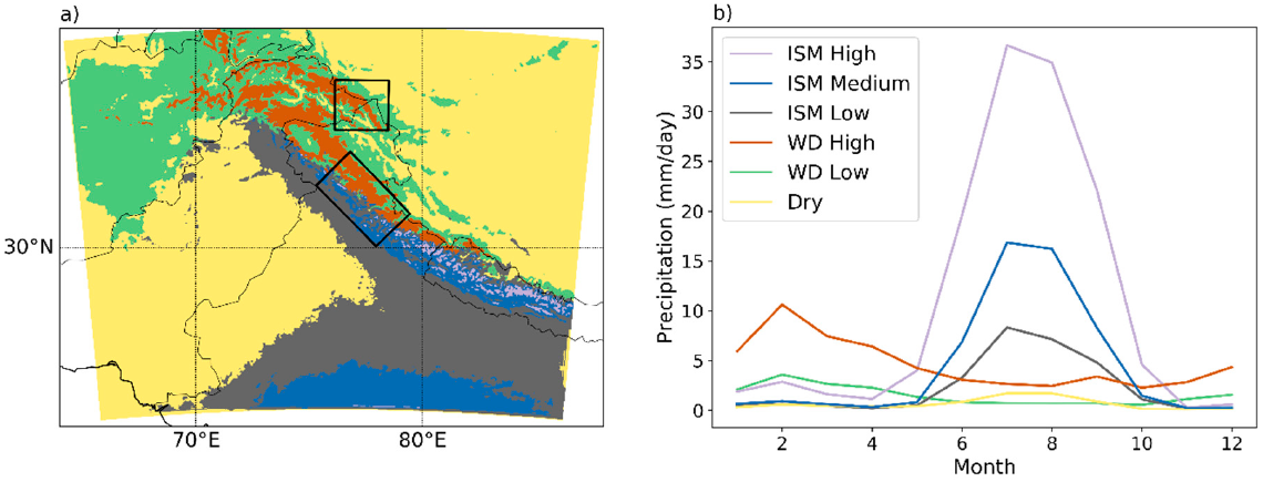
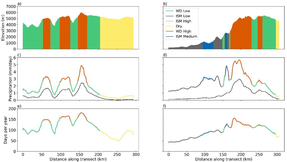
3.1. Regional Precipitation Seasonality and Topographic Effects

To identify regions dominated by ISM (Indian Summer Monsoon) and WD (westerly disturbances), we applied k-means clustering to climatological monthly mean precipitation time series at each WRF grid point, and present results for k = 6 clusters. Three clusters had an annual cycle dominated by the ISM (ISM High, Medium, and Low), two had an annual cycle dominated by WDs (WD High and Low), and one represented regions with low annual precipitation (Dry) (Figure 3a). Clusters that follow the same annual cycle of precipitation (e.g., ISM High, Medium, and Low) are differentiated by precipitation magnitude (Figure 3b). The analysis reveals a more complex spatial pattern than a simple east–west gradient in precipitation amount and seasonality. In the Himalayan foothills and adjoining lowlands, ISM precipitation dominates as far west as Pakistan. WD precipitation dominates the mountains of Afghanistan and the Karakoram, but persists in pockets near and along the Himalayan crest as far east as Nepal. Although lowland areas of western India, Pakistan, and the Tibetan Plateau receive most of their precipitation during the ISM, the quantities are small enough that these regions are in the dry cluster.

The complex spatial pattern in precipitation statistics suggests a strong role for topography in controlling the magnitude and seasonality of precipitation. To further investigate these relationships, we examine precipitation amount and frequency across transects normal to the topography within the Karakoram and western Himalaya (Figure 4; transects shown in Figure 1). Values were calculated at 2-km intervals along each transect, averaging all WRF grid points within a 5-km radius. Along the transect, assignment to clusters (WD low, dry, etc.) was based on the mode of the clusters present in the 5-km radius.

The transects show that the k-means clustering results in Figure 2 are strongly linked to the terrain. In the Karakoram, valleys fall into the WD Low cluster, peaks into the WD High cluster, and areas northeast of the crest into the Dry cluster (Figure 4a). In the western Himalaya, the plains and foothills are in ISM Low and ISM Medium, before transitioning to WD Low and High at higher elevations. The effect of topography on the clusters is explained by the apparent relationships between topography and precipitation in each region. In the Karakoram, precipitation magnitude and frequency both maximize over the mountain crests (Figure 4c,e), with valleys having significantly less precipitation and lower frequency precipitation as compared to the peaks. This suggests that weather stations dominantly located in valleys are not representative of the surrounding higher elevation terrain and may underestimate precipitation magnitude and frequency in the mountains. Further northeast of the Karakoram the climate is drier, with infrequent precipitation. Precipitation along the Himalayan transect also shows a distinct, yet more complex, relationship with topography (Figure 4d,f). Seasonality shifts from ISM to WD between the foothills and high Himalayas., and both precipitation amount and frequency peak in the western Himalaya before reaching the crest of the terrain. Similar to the Karakoram, precipitation amount and frequency are lower in the surrounding valleys of the western Himalaya.

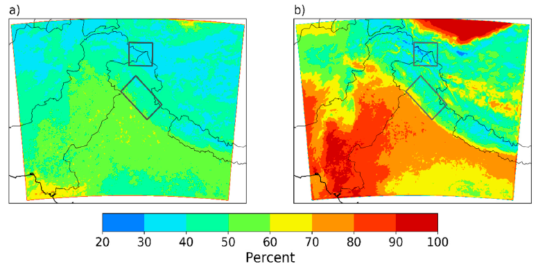
3.2. Cluster Precipitation Statistics and Role of Large Precipitation Events

The elevation transects illustrate a strong relationship between the precipitation clusters and topography, and suggest the clusters represent the spatial and temporal variations in precipitation climatology across the region well. However, there is significant variability within clusters. Here we analyze the distribution of several precipitation variables at all grid points within the six clusters (Figure 5a–d) and at upper-elevation grid points (above 3000 m; Figure 5e–h). Consistent with what might be inferred from Figure 3b, the median annual average precipitation for all grid points in each cluster is lowest in Dry, increases from WD Low to WD High, and increases from ISM Low to ISM Med to ISM High. Similar results are found for upper-elevation grid points (Figure 5c,g). Median precipitation in ISM Med and High exceeds that in WD High, consistent with greater annual precipitation in regions strongly influenced by the ISM. Annual precipitation tends to be positively skewed in all clusters and is largest in ISM high and varies from 5.4 to 27 mm d⁻¹ at upper-elevation grid points.

The median frequency of precipitation days (i.e., days with ≥0.25 mm) is similarly lowest in Dry, increases from WD Low to WD High, and increases from ISM Low to ISM Med to ISM High (Figure 5d,h). There is, however, large intracluster variability with a range > 100 days in all clusters, and interquartile ranges from 13.5 days in ISM Low to 52.5 in WD low. To illustrate the contribution of the largest precipitation days, we present the percentage of annual precipitation produced by the upper-decile precipitation days (Figure 5a,e). This contribution shows remarkably little variability within clusters and the difference between clusters is relatively small with the smallest mean contribution (38%) in ISM High and the largest in ISM Low (53%) (Figure 5c). Precipitation days are often associated with “events” occurring over multiple days. To quantify the role of multiday precipitation events over the HMA region, precipitation was analyzed using a 4-day temporal window. The window size was chosen through an analysis of correlations between precipitation at a given time, and precipitation n hours later, which showed that at around n = 96 h, the correlations dropped to the same level as seasonal noise, indicating that many precipitation events in the region last 4 days or less. Thus, for this study, a “precipitation day” is defined as any day with precipitation greater than 0.25 mm, and a “96-h precipitation event” is defined as precipitation over a 4-day window. The percentage of annual precipitation produced during the five largest precipitation events (Figure 5b,f) follows a similar pattern as that of the upper-decile precipitation days, albeit with increased inter- and intra-cluster variance.

Mapping the percentage of annual precipitation produced by upper-decile days shows some relationship to orography and elevation with values greatest across the Indo–Gangetic Plain (generally >50% with >60% in some localized regions) decreasing to ~40–50% in the western Himalaya and decreasing further to <40% in the highest altitude regions of the Karakoram (Figure 6a). The percentage of annual precipitation produced during the five largest 96-h precipitation events each year generally follows a similar spatial pattern, but the difference between lowlands and mountains is more pronounced with values > 80% over the Indo-Gangetic Plain, but <30% over portions of the western Himalaya and Karakoram (Figure 6b). In addition, there is a sharper contrast between lower and upper-elevation regions within the western Himalaya and Karakoram. Thus, although prior works suggests that large storms contribute a large portion of precipitation in the Karakoram and western Himalaya [19,28,48], the importance of these multi-day events decreases at upper elevations where more frequent events contribute a greater fraction of the annual precipitation.

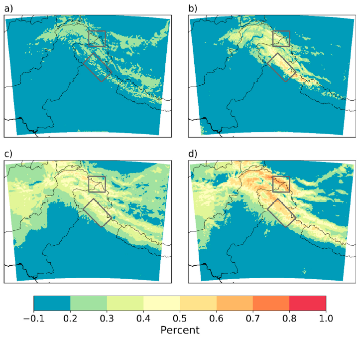
3.3. IWV, IVT, and Precipitation

WDs and ISM surges can transport moisture from the Arabian Sea, Bay of Bengal, and Indian Ocean, leading to large IVT to the mountains of HMA. Pearson correlation coefficients between hourly WRF precipitation and IWV and IVT are generally low (absolute value < 0.2) over the Indo–Gangetic Plain, but more strongly positive over HMA (Figure 7). Over HMA, the positive correlation with precipitation is larger for IVT than IWV (cf. Figure 5a–d), consistent with findings at upper elevations of the western United States [44] (see their Figure 2). Additionally, correlations are higher during the cool season (December to March) than the warm season (cf. Figure 7a–d). The largest correlations occur for IVT over the upper elevations of the western Himalaya and Karakoram during the cool season when values reach >0.6 and >0.7 over each region, respectively (Figure 7d). These high correlations indicate that IVT may be valuable for understanding the cool-season precipitation climate of these regions, including extreme precipitation events. In comparison, lower correlations are found in the eastern Himalaya where convective systems play a greater role [49].

Based on hourly model output, Figure 8 summarizes the areal-averaged vector-mean IVT direction frequency (a,d), vector-mean IVT magnitude (b,e), and precipitation rate (d,f) within the Karakoram and western Himalaya subregions as a function of time of year and vector-mean IVT direction. This figure illustrates the variations in the relationship between precipitation and IVT throughout the year, and also seasonal changes in moisture flux direction within a region. In the Karakoram, IVT occurs most frequently from the southwest-west (~215–270°) in all seasons. From September–May, IVT magnitude and precipitation are greatest for IVT from the south-southwest (~180–245°), although these distributions feature a tail that includes northwest and northerly directions. During the ISM from June–August, IVT magnitudes are greater, but precipitation exhibits no clear IVT direction preference. In the western Himalaya from September–May, the IVT occurs across a wide range of directions and is most common from southeast to northwest (~155–325°). During the ISM from June–August, a bimodal distribution exists with peaks from the southeast (~145°) and northwest (~305°). From September–May, IVT magnitude and precipitation tend to be highest for IVT from the southeast-southwest (~135–225°). During the ISM from June–August, the IVT magnitude distribution is bimodal with peaks for IVT from the south-southeast (~155°) and west-northwest (~295°). The precipitation distribution is quite broad during this period, but is greatest for IVT from the southeast to southwest (~135–225°). These results illustrate the seasonal relationships between IVT and precipitation in the two regions. During the cool season, precipitation in the Karakoram and western Himalaya maximizes for IVT from the south-southwest and southeast-southwest, respectively. These are directions that appear to enable large IVT magnitudes with a substantial cross-barrier component. During the ISM, precipitation in the Karakoram is not strongly related to IVT direction, consistent with the greater role convection plays in precipitation generation. Similarly, ISM precipitation over the western Himalaya also features a broader distribution with IVT direction, although there is a peak for IVT from the southeast to southwest.

Another perspective on the relationship between IVT and precipitation in the two regions is provided by the water budget statistics presented in Figure 9. Here, calculations are based on 96-h windows to capture relationships between vapor transport and the 96-h precipitation events in the two target regions. In the Karakoram, the IVT frequency for all periods has a fairly narrow distribution centered on west-southwest (250°), whereas the distribution in the western Himalaya is broader and peaks at west-northwest (305°) with a long tail toward southerly directions. During the largest 96-h precipitation events (i.e., those in the top five annually), however, the IVT is most common from the southwest (230°) over the Karakoram and the south (180°) over the western Himalaya, although the distribution is broad over the latter. Drying ratios, which measure the fraction of incoming water vapor converted to precipitation, similarly maximize for IVT from the southwest (~225°) over the Karakoram and south (180°) over the western Himalaya. Thus, the largest precipitation events and most efficient conversion of incoming water vapor into precipitation occurs for IVT from the southwest over the Karakoram and south over the western Himalaya.

Figure 10 shows the seasonality and IVT direction during the 96-h precipitation events in the western Himalaya (Figure 10a) and Karakoram (Figure 10b). Large events in the western Himalaya occur at a similar frequency in the warm and cool seasons, but rarely in the intermediate seasons, whereas those in the Karakoram occur mainly in the cool season and intermediate months. Events in all seasons are more tightly clustered in terms of moisture transport direction in the Karakoram than the western Himalaya, which experiences a wider range of moisture transport directions. Additionally, moisture transport directions shift to the southeast over the western Himalaya during the ISM. The ability of this methodology to capture regional-scale patterns in moisture transport that lead to intense precipitation provides a way to link the results of high-resolution modeling to those at a lower resolution, where the latter could accurately resolve the mean direction of moisture transport, but not necessarily intense precipitation in mountainous regions.

4. Discussion and Conclusions

This work uses 4-km WRF simulations to quantify multiple aspects of the precipitation climatology of the Indus River basin region of High Mountain Asia (HMA), notably the transition between monsoon and winter precipitation dominated areas, and the contribution of large events to annual precipitation. The k-means classification based on monthly precipitation reveals a more complex pattern than a simple east–west transition between monsoon and WD dominated areas, due to the influence of complex terrain. For example, Indian Summer Monsoon (ISM) dominated precipitation occurs as far west as Pakistan in the Himalayan foothills and adjoining lowlands, whereas Westerly Disturbance (WD) dominated precipitation persists in pockets near and along the Himalayan crest as far east as Nepal. This pattern is similar to that found by Curio and Scherer [23] and Maussion et al. [22]. However, Maussion et al. [22] focused on precipitation over glacier areas. Our results expand this to the full region, providing more detailed spatial analysis of precipitation statistics beyond glacierized areas. Curio and Scherer [23] also analyze the larger region; however, they use the monthly proportion of total annual precipitation, and thus focus only on precipitation seasonality. The cluster analysis in the present study uses total precipitation amount, which allows for comparisons of both precipitation seasonality and magnitude, and how these correspond to changes in precipitation frequency and the impact of large events.

We analyze transects across the Karakoram and western Himalaya to further elucidate the relationship between precipitation and topography in HMA. In the Karakorum, precipitation amount and frequency increase with elevation, maximizing over mountain crests. A more complex relationship exists in the western Himalaya where precipitation amount and frequency peak before reaching the crest of the terrain. In addition, the seasonality in precipitation shifts between the foothills of the Himalayas and the Himalaya proper. This highlights a distinct difference in the relationship between topography and precipitation statistics in the Himalayas versus the Karakoram. The results also suggest precipitation observations from valleys are not always representative of the magnitude, frequency, or seasonality of nearby high elevation regions. In addition, this further supports previous work [21,22,23,26] that highlight the importance of model resolution in capturing the magnitude, frequency and seasonality of precipitation in complex terrain. While higher-resolution models do not automatically result in improved accuracy of precipitation statistics, they have improved terrain resolution which allows for more detailed analyses of the relationship between precipitation and topography.

The contribution of upper decile days and five largest 96-h precipitation events each year to annual precipitation also varies with terrain. A strong elevation contrast exists for these days and events, with the latter contributing more than 80% of the annual precipitation at the low elevations of the Indo-Gangetic Plain, but less than 30% over much of the Karakoram and western Himalaya. This elevation dependence is also evident, albeit slightly more muted, for upper decile precipitation days. These results contrast with previous work that suggests large storms contribute a larger portion of precipitation in the Karakoram and western Himalaya [19,28,42]. Our results show decreasing importance of large precipitation events with increasing elevation where smaller, more frequent precipitation events contribute a greater fraction of the annual precipitation.

Correlations between precipitation and moisture variables add additional evidence that IVT is a valuable variable for understanding the precipitation climate of the Karakorum and western Himalaya. In particular, the correlation between precipitation and IVT increases with elevation, exceeding 0.7 in some areas of the Karakoram and 0.6 in some areas of the western Himalaya. These results are similar to those found by Curio and Scherer [23], but show much lower correlation values in the deep mountain valleys of the western Himalaya and Karakoram. The largest 96-h precipitation events and the greatest precipitation efficiency, as quantified by the drying ratio, maximize for IVT directed from the southwest over the Karakorum. In contrast, the largest 96-h precipitation events over the western Himalaya occur for a broader range of IVT orientations, indicating a more diverse storm climatology, although there is a peak in the largest 96-h precipitation events and precipitation efficiency for IVT directed from the south. These results suggest that high-resolution climate modeling can capture regional conditions that lead to intense precipitation, and could allow for a link between synoptic scale patterns captured in global climate models and reanalysis products similar to Cannon et al. [19].

Dars et al. [30] show that their higher-resolution WRF simulations more accurately represent precipitation and temperature than their coarser-resolution simulations. We utilized the highest resolution simulations (4-km) to minimize uncertainties and capture smaller-scale variability in orographic precipitation, but significant seasonal biases in both precipitation and temperature were noted. This bias may lead to an over-estimation of the cool season precipitation contribution to annual precipitation and over-steepened topographic gradients in precipitation seasonality. Despite these potential biases, this model and others appear to capture the overall precipitation patterns that impact the region [22,25,27,34,47]. Thus, while exact magnitudes and specific spatial details of the current study are uncertain and model-dependent, the big picture results are likely robust.

Overall, these results have revealed a level of small-scale spatial variability and terrain dependence, not just in precipitation magnitude and frequency, but in seasonality, that goes unresolved in some coarser gridded products for the region. This provides a basis for further work continuing to produce and utilize high resolution modeling to study small-scale variations in climate in this region and better understand how this granularity impacts water resource issues for downstream populations.

References

1. Barnett, T.P.; Adam, J.C.; Lettenmaier, D.P. Potential impacts of a warming climate on water availability in snow-dominated regions. Nature 2005, 438, 303–309. [Google Scholar] [CrossRef] [PubMed]
2. Immerzeel, W.W.; Lutz, A.F.; Andrade, M.; Bahl, A.; Biemans, H.; Bolch, T.; Hyde, S.; Brumby, S.; Davies, B.J.; Elmore, A.C.; et al. Importance and vulnerability of the world’s water towers. Nature 2020, 577, 364–369. [Google Scholar] [CrossRef] [PubMed]
3. Singh, P.; Jain, S.K.; Kumar, N. Estimation of snow and glacier-melt contribution to the Chenab river, Western Himalaya. Mt. Res. Dev. 1997, 17, 49–56. [Google Scholar] [CrossRef]
4. Biemans, H.; Siderius, C.; Lutz, A.F.; Nepal, S.; Ahmad, B.; Hassan, T.; von Bloh, W.; Wijngaard, R.R.; Wester, P.; Shrestha, A.B.; et al. Importance of snow and glacier meltwater for agriculture on the Indo-Gangetic Plain. Nat. Sustain. 2019, 2, 594–601. [Google Scholar] [CrossRef]
5. Loomis, B.D.; Richey, A.S.; Arendt, A.A.; Appana, R.; Deweese, Y.-J.C.; Forman, B.A.; Kumar, S.V.; Sabaka, T.J.; Shean, D.E. Water storage trends in High Mountain Asia. Front. Earth Sci. 2019, 7. [Google Scholar] [CrossRef]
6. Fowler, H.J.; Archer, D.R. Conflicting signals of climatic change in the Upper Indus Basin. J. Clim. 2006, 19, 4276–4293. [Google Scholar] [CrossRef] [Green Version]
7. Winiger, M.; Gumpert, M.; Yamout, H. Karakorum–Hindukush–western Himalaya: Assessing high-altitude water resources. Hydrol. Process. 2005, 19, 2329–2338. [Google Scholar] [CrossRef]
8. Rasmussen, R.; Baker, B.; Kochendorfer, J.; Meyers, T.; Landolt, S.; Fischer, A.P.; Black, J.; Thériault, J.M.; Kucera, P.; Gochis, D.; et al. How well are we measuring snow: The NOAA/FAA/NCAR winter precipitation test bed. Bull. Am. Meteorol. Soc. 2012, 93, 811–829. [Google Scholar] [CrossRef] [Green Version]
9. Kumar, S.; Gil, G.S.; Santoch, S. Spatial distribution of rainfall with elevation in Satluj river basin: 1986–2010, Himachal Pradesh, India. World Sci. News 2015, 57, 163–175. [Google Scholar] [CrossRef] [Green Version]
10. Shi, Y. Characteristics of late Quaternary monsoonal glaciation on the Tibetan Plateau and in East Asia. Quat. Int. 2002, 97–98, 79–91. [Google Scholar] [CrossRef]
11. Krishnamurti, T.N.; Kishtawal, C.M. A pronounced continental-scale diurnal mode of the Asian summer monsoon. Mon. Weather Rev. 2000, 128, 462–473. [Google Scholar] [CrossRef]
12. Syed, F.S.; Giorgi, F.; Pal, J.S.; King, M.P. Effect of remote forcings on the winter precipitation of central southwest Asia part 1: Observations. Theor. Appl. Climatol. 2006, 86, 147–160. [Google Scholar] [CrossRef]
13. Dimri, A.P.; Niyogi, D.; Barros, A.P.; Ridley, J.; Mohanty, U.C.; Yasunari, T.; Sikka, D.R. Western disturbances: A review. Rev. Geophys. 2015, 53, 225–246. [Google Scholar] [CrossRef]
14. Palazzi, E.; von Hardenberg, J.; Provenzale, A. Precipitation in the Hindu-Kush Karakoram Himalaya: Observations and future scenarios. J. Geophys. Res. Atmos. 2013, 118, 85–100. [Google Scholar] [CrossRef]
15. You, Q.; Fraedrich, K.; Ren, G.; Ye, B.; Meng, X.; Kang, S. Inconsistencies of precipitation in the eastern and central Tibetan Plateau between surface adjusted data and reanalysis. Theor. Appl. Climatol. 2012, 109, 485–496. [Google Scholar] [CrossRef]
16. Bashir, F.; Zeng, X.; Gupta, H.; Hazenberg, P. A hydrometeorological perspective on the Karakoram anomaly using unique valley-based synoptic weather observations. Geophys. Res. Lett. 2017, 44, 10470–10478. [Google Scholar] [CrossRef] [Green Version]
17. Bharti, V.; Singh, C. Evaluation of error in TRMM 3B42V7 precipitation estimates over the Himalayan region. J. Geophys. Res. Atmos. 2015, 120, 12458–12473. [Google Scholar] [CrossRef]
18. Smith, T.; Bookhagen, B. Remotely sensed rain and snowfall in the Himalaya. In Himalayan Weather and Climate and Their Impact on the Environment; Springer: Cham, Germany, 2020; pp. 119–139. ISBN 978-3-030-29683-4. [Google Scholar]
19. Cannon, F.; Carvalho, L.M.V.; Jones, C.; Bookhagen, B. Multi-Annual variations in winter westerly disturbance activity affecting the Himalaya. Clim. Dyn. 2015, 44, 441–455. [Google Scholar] [CrossRef] [Green Version]
20. Lang, T.J.; Barros, A.P. Winter storms in the Central Himalayas. J. Meteorolog. Soc. Jpn. 2004, 82, 829–844. [Google Scholar] [CrossRef] [Green Version]
21. Bolch, T.; Kulkarni, A.; Kääb, A.; Huggel, C.; Paul, F.; Cogley, J.G.; Frey, H.; Kargel, J.S.; Fujita, K.; Scheel, M.; et al. The state and fate of Himalayan glaciers. Science 2012, 336, 310–314. [Google Scholar] [CrossRef] [PubMed] [Green Version]
22. Maussion, F.; Scherer, D.; Mölg, T.; Collier, E.; Curio, J.; Finkelnburg, R. Precipitation seasonality and variability over the Tibetan Plateau as resolved by the High Asia Reanalysis. J. Clim. 2014, 27. [Google Scholar] [CrossRef] [Green Version]
23. Curio, J.; Scherer, D. Seasonality and spatial variability of dynamic precipitation controls on the Tibetan Plateau. Earth Syst. Dynam. 2016, 7, 767–782. [Google Scholar] [CrossRef] [Green Version]
24. Pritchard, D.M.W.; Forsythe, N.; Fowler, H.J.; O’Donnell, G.M.; Li, X.-F. Evaluation of upper indus near-surface climate representation by WRF in the High Asia Refined Analysis. J. Hydrometeorol. 2019, 20, 467–487. [Google Scholar] [CrossRef]
25. Wang, X.; Tolksdorf, V.; Otto, M.; Scherer, D. WRF-Based dynamical downscaling of ERA5 reanalysis data for High Mountain Asia: Towards a new version of the High Asia Refined analysis. Int. J. Climatol. 2020, 41. [Google Scholar] [CrossRef]
26. Hamm, A.; Arndt, A.; Kolbe, C.; Wang, X.; Thies, B.; Boyko, O.; Regiani, P.; Scherer, D.; Bendix, J.; Schneider, C. Intercomparison of gridded precipitation datasets over a sub-region of the Central Himalaya and the Southwestern Tibetan Plateau. Water 2020, 12, 3271. [Google Scholar] [CrossRef]
27. Bonekamp, P.N.J.; Collier, E.; Immerzeel, W.W. The impact of spatial resolution, land use, and spinup time on resolving spatial precipitation patterns in the Himalayas. J. Hydrometeorol. 2018, 19, 1565–1581. [Google Scholar] [CrossRef] [Green Version]
28. Qiu, J. The third pole. Nature 2008, 454, 393–396. [Google Scholar] [CrossRef] [Green Version]
29. Mukhopadhyay, B.; Khan, A. A quantitative assessment of the genetic sources of the hydrologic flow regimes in Upper Indus Basin and its significance in a changing climate. J. Hydrol. 2014, 509, 549–572. [Google Scholar] [CrossRef]
30. Dars, G.H.; Strong, C.; Kochanski, A.K.; Ansari, K.; Ali, S.H. The spatiotemporal variability of temperature and precipitation over the upper Indus Basin: An evaluation of 15 year WRF simulations. Appl. Sci. 2020, 10, 1765. [Google Scholar] [CrossRef] [Green Version]
31. Skamarock, W.C.; Klemp, J.B.; Dudhia, J.; Gill, D.O.; Barker, D.M.; Duda, M.G.; Huang, X.-Y.; Wang, W.; Powers, J.G. A Description of the Advanced Research WRF Version 3; NCAR Technical Note NCAR/TN-475+STR; NCAR: Boulder, CO, USA, 2008. [Google Scholar]
32. Saha, S.; Moorthi, S.; Pan, H.L.; Wu, X.; Wang, J.; Nadiga, S.; Tripp, P.; Kistler, R.; Woollen, J.; Behringer, D.; et al. The NCEP climate forecast system reanalysis. Bull. Am. Meteorol. Soc. 2010, 91, 1015–1057. [Google Scholar] [CrossRef]
33. Ikeda, K.; Rasmussen, R.; Liu, C.; Gochis, D.; Yates, D.; Chen, F.; Tewari, M.; Barlage, M.; Dudhia, J.; Miller, K.; et al. Simulation of seasonal snowfall over Colorado. Atmos. Res. 2010, 97, 462–477. [Google Scholar] [CrossRef]
34. Maussion, F.; Scherer, D.; Finkelnburg, R.; Richters, J.; Yang, W.; Yao, T. WRF simulation of a precipitation event over the Tibetan Plateau, China—An assessment using remote sensing and ground observations. Hydrol. Earth Syst. Sci. 2011, 15, 1795–1817. [Google Scholar] [CrossRef] [Green Version]
35. Niu, G.-Y.; Yang, Z.-L.; Mitchell, K.E.; Chen, F.; Ek, M.B.; Barlage, M.; Kumar, A.; Manning, K.; Niyogi, D.; Rosero, E.; et al. The community Noah land surface model with multiparameterization options (Noah-MP): 1. Model description and evaluation with local-scale measurements. J. Geophys. Res. Atmos. 2011, 116. [Google Scholar] [CrossRef] [Green Version]
36. Hong, S.-Y.; Noh, Y.; Dudhia, J. A new vertical diffusion package with an explicit treatment of entrainment processes. Mon. Weather Rev. 2006, 134, 2318–2341. [Google Scholar] [CrossRef] [Green Version]
37. Thompson, G.; Field, P.R.; Rasmussen, R.M.; Hall, W.D. Explicit forecasts of winter precipitation using an improved bulk microphysics scheme. Part II: Implementation of a new snow parameterization. Mon. Weather Rev. 2008, 136, 5095–5115. [Google Scholar] [CrossRef]
38. Iacono, M.J.; Delamere, J.S.; Mlawer, E.J.; Shephard, M.W.; Clough, S.A.; Collins, W.D. Radiative forcing by long-lived greenhouse gases: Calculations with the AER radiative transfer models. J. Geophys. Res. Atmos. 2008, 113, 2–9. [Google Scholar] [CrossRef]
39. Dudhia, J. Numerical study of convection observed during the winter monsoon experiment using a mesoscale two-dimensional model. J. Atmos. Sci. 1989, 46, 3077–3107. [Google Scholar] [CrossRef]
40. Kain, J.S. The Kain—Fritsch convective parameterization: An update. J. Appl. Meteorol. 2004, 43, 170–181. [Google Scholar] [CrossRef] [Green Version]
41. Doswell, C.A., III; Brooks, H.E.; Maddox, R.A. Flash flood forecasting: An ingredients-based methodology. Weather Forecast. 1996, 11, 560–581. [Google Scholar] [CrossRef]
42. Ralph, F.M.; Coleman, T.; Neiman, P.J.; Zamora, R.J.; Dettinger, M.D. Observed impacts of duration and seasonality of atmospheric-river landfalls on soil moisture and runoff in coastal Northern California. J. Hydrometeorol. 2013, 14, 443–459. [Google Scholar] [CrossRef] [Green Version]
43. Neiman, P.J.; Ralph, F.M.; Wick, G.A.; Lundquist, J.D.; Dettinger, M.D. Meteorological characteristics and overland precipitation impacts of atmospheric rivers affecting the west coast of North America based on eight years of SSM/I satellite observations. J. Hydrometeorol. 2008, 9, 22–47. [Google Scholar] [CrossRef]
44. Rutz, J.J.; Steenburgh, W.J.; Ralph, F.M. climatological characteristics of atmospheric rivers and their inland penetration over the western United States. Mon. Weather Rev. 2014, 142, 905–921. [Google Scholar] [CrossRef]
45. Froidevaux, P.; Martius, O. Exceptional integrated vapour transport toward orography: An important precursor to severe floods in Switzerland. Q. J. R. Meteorolog. Soc. 2016, 142, 1997–2012. [Google Scholar] [CrossRef] [Green Version]
46. Thapa, K.; Endreny, T.A.; Ferguson, C.R. Atmospheric rivers carry nonmonsoon extreme precipitation into Nepal. J. Geophys. Res. Atmos. 2018, 123, 5901–5912. [Google Scholar] [CrossRef]
47. Curio, J.; Maussion, F.; Scherer, D. A 12-year high-resolution climatology of atmospheric water transport over the Tibetan Plateau. Earth Syst. Dynam. 2015, 6, 109–124. [Google Scholar] [CrossRef] [Green Version]
48. Norris, J.; Carvalho, L.; Jones, C.; Cannon, F. WRF simulations of two extreme snowfall events associated with contrasting extratropical cyclones over the western and central Himalaya. J. Geophys. Res. 2010, 120, 3114–3138. [Google Scholar] [CrossRef] [Green Version]
49. Medina, S.; Houze, R.A., Jr.; Kumar, A.; Niyogi, D. Summer monsoon convection in the Himalayan region: Terrain and land cover effects. Q. J. R. Meteorolog. Soc. 2010, 136, 593–616. [Google Scholar] [CrossRef] [Green Version]
Figure 1. WRF domains (red, blue, and black boxes), Karakoram and western Himalaya subregions used for detailed analysis (green boxes), transects (black dashed lines), and 9 arc-second relief of HMA (m, shaded following inset scale).
Atmosphere 12 00355 g001
Figure 2. Variance as a function of the number of clusters (k) used in the k-means clustering, expressed as a portion of the total variance of the dataset. The red vertical line represents the number of clusters chosen for analysis.
Atmosphere 12 00355 g002
Figure 3. Precipitation regimes identified by k-means clustering (a), and the mean monthly precipitation (mm d−1) time series for the centroid of each cluster (b). Black boxes in (a) indicate Karakoram (top) and western Himalaya (center) subregions. The colors in the legend in (b) apply to both panels.
Atmosphere 12 00355 g003
Figure 4. Transects through the Karakoram (left) and western Himalaya (right), showing elevation (a,b), precipitation (with cool season (December–March) precipitation in black) (c,d), and precipitation frequency (e,f). Lines are colored according to the mode of the K-means cluster along the transect, with the same color scheme as Figure 2. Both transects run from southwest to northeast and are shown in Figure 1.
Atmosphere 12 00355 g004
Figure 5. Box-and-whisker plots displaying 90th percentile contribution, top 5 event contribution, annual precipitation, and precipitation frequency for each cluster in the K-means clustering (left panels) and for elevations >3000 m for each cluster (right panels). Orange line indicates median, box the interquartile range, the lower whisker at Q1—1.5*IQR, upper whisker at Q3 + 1.5*IQR (where Q1 is the 25th percentile value, Q3 is the 75th percentile value, and IQR is the interquartile range), and circles outliers. (a) 90th percentile; (b) top 5 events; (c) annual precipitation; (d) precipitation frequency; (e) 90th percentile (>3000 m); (f) top 5 events (>3000 m); (g) annual precipitation (>3000 m); (h) precipitation frequency (>3000 m).
Atmosphere 12 00355 g005
Figure 6. Percentage of annual precipitation produced during and (a) top-decile precipitation days in each year and (b) the 5 largest 96-h precipitation events. Boxes indicate Karakoram (top) and western Himalaya (center) subregions.
Atmosphere 12 00355 g006
Figure 7. Pearson correlation coefficients between precipitation and (a) warm-season (June–September) IWV, (b) warm-season IVT, (c) cool-season (December–March) IWV, and (d) cool-season IVT. All correlations are calculated based on hourly data. Grey boxes indicate Karakoram (top) and western Himalaya (center) subregions.
Atmosphere 12 00355 g007
Figure 8. Vector-mean IVT direction frequency (a,d), vector-mean IVT magnitude (b,e), and mean precipitation amount (c,f) in the Western Himalaya (ac) and Karakoram (df) subregions as a function of time of year (y-axis) and IVT direction (x-axis) to show the relationship between moisture source direction, IVT magnitude, and precipitation. All panels are calculated from hourly values; cells with less than 10 occurrences over the 15-year period excluded (grey regions). The Karakoram and western Himalaya subregions of focus here are outlined as black boxes in Figure 3, Figure 6 and Figure 7.
Atmosphere 12 00355 g008
Figure 9. For the Karakoram (blue) and western Himalaya (red), 96-h IVT frequency for the entire 15-year study period (dashed lines), the relative frequency of the largest annual IVT events (top 5 per year, 80 total) (color fill), and drying ratio (solid lines). Bin width for IVT direction is 20°. The Karakoram and western Himalaya subregions of focus here are outlined as black boxes in Figure 3, Figure 6 and Figure 7.
Atmosphere 12 00355 g009
Figure 10. The relative frequency of the largest 96-h precipitation events (top 5 per year, 80 total) in the western Himalaya (a) and Karakoram (b) using bin width of 20 degrees along the x-axis. This is similar to the shaded areas in Figure 7, but here storms are separated into cool season (December–March), warm season (June–September), and intermediate seasons (April, May, October, November).
Atmosphere 12 00355 g010