
Atlantic Hurricane Activity Prediction: A Machine Learning Approach


1
Department of Electrical and Computer Engineering, North Carolina State University, Raleigh, NC 27695-8208, USA
2
Department of Marine, Earth, and Atmospheric Sciences, North Carolina State University, Raleigh, NC 27695-8208, USA
*
Author to whom correspondence should be addressed.
Atmosphere 2021, 12(4), 455; https://0-doi-org.brum.beds.ac.uk/10.3390/atmos12040455
Submission received: 28 February 2021
/
Revised: 29 March 2021
/
Accepted: 1 April 2021
/
Published: 3 April 2021
(This article belongs to the Special Issue Recent Advances and Future Prospects of Machine Learning in Predictive Modeling of Atmospheric Sciences)
Abstract
:Long-term hurricane predictions have been of acute interest in order to protect the community from the loss of lives, and environmental damage. Such predictions help by providing an early warning guidance for any proper precaution and planning. In this paper, we present a machine learning model capable of making good preseason-prediction of Atlantic hurricane activity. The development of this model entails a judicious and non-linear fusion of various data modalities such as sea-level pressure (SLP), sea surface temperature (SST), and wind. A Convolutional Neural Network (CNN) was utilized as a feature extractor for each data modality. This is followed by a feature level fusion to achieve a proper inference. This highly non-linear model was further shown to have the potential to make skillful predictions up to 18 months in advance.
1. Introduction
A tropical cyclone (TC) is a rotating storm system over the tropical ocean. Its strength and location earn it different names. The strength of a cyclone is categorized by maximum wind-speed at a given time. A TC can be either a Depression, a Tropical Storm (TS), a Hurricane or a Major Hurricane as its strength increases. Within the Northern Atlantic and Eastern Pacific basins, a tropical cyclone with wind speeds of over 65 knots is called a hurricane. Our focus in this work is on the hurricanes in the North Atlantic basin, where the season starts on 1 June each year and ends on 30 November. Although TCs may occur outside the hurricane season, such occurences are rare.
Each year TCs wreak havoc on coastal regions around the world. Before the advent of powerful satellites to observe TC tracks from up in space, very few tools were available to monitor them in real-time, let alone forecast their occurrences in advance. As data collection and assimilation methods in weather science have matured, detailed short-term track and intensity predictions now can be made up to a week in advance. This has helped to bring down casualty rates by planning rapid evacuation efforts. The short prediction window, however, can only moderately mitigate the often entailing severe economic damage. If accurate and substantially earlier predictions of the level of TC activities such as storm counts and accumulated cyclone energy (ACE) levels are done, the various organizations can as a result, make a well thought out and proper long term economic and urban plan to further mitigate losses of lives and property.
A number of mathematical models, commonly referred to as Numerical Weather Prediction(NWP) models, have been developed and refined in the last few decades [1]. They often simulate various complex oceanic and atmospheric interactions to make short term predictions of a few hours to days in advance, and less detailed climate predictions of months to years in advance. Statistical regression models have also been developed to make long term predictions [2,3,4]. However, the immense complexity, size and dynamic nature of weather systems collectively pose a significant challenge to achieving high accuracy and precision. NWP methods are computationally intensive and regression-based methods require discovery of hand-crafted predictors. Given the vast amount of high resolution raw data available due to advances in weather science, machine learning (ML) based techniques also provide powerful methods for weather prediction. ML has been applied in recent years to make short term predictions on TCs with comparable performance to NWP systems. Application of ML methods to make long term forecasts remains, however, more challenging on account of paucity of ground truth data.
The problem of TC prediction can be broadly classified into two classes:
- Short term predictions: These are generally made 6 h to 7 days in advance. The predictands are spatio-temporal quantities, such as track and intensity of an individual cyclone.
- Long term predictions: These are seasonal forecasts generally made at least a month in advance. The predictands are one-dimensional time series like the total number of cyclones and Accumulated Cyclone Energy (ACE) in a basin (see Section 4 for details). Generally, certain handcrafted climatological indices are used as predictors.
While we have a vastly rich amount of modality data (related to pressure, temperature, wind speed etc) at our disposal, the ground truth data, such as the number of cyclones in each month or year, or their intensity is very sparse. As a result, ML methods which generally require large amount of data for training, suffer. ML based models project data into high dimensional spaces. As the dimensionality of the space increases the sparsity of projected data also increases exponentially, reducing the predictive power of the model [5]. We address this challenge by oversampling our ground truth data (see Section 4 for details).
We propose, in this sequel, a Fused CNN architecture which uses the data from various modalities like sea level pressure, sea surface temperature, wind speed etc to capture long term predictions on some well-known one-dimensional indices which are well correlated with hurricane activity. Roheda et al. [6] have developed a multi-modality feature fusion based model to detect faulty sensors in an environment embedded with multiple heterogeneous sensors. Robust decision-level fusion has also been demonstrated earlier [7]. Our model was shown to achieve a comparable prediction accuracy as other state of the art statistical methods at longer lead times. Making long term predictions with assimilated modality data instead of climatological indices will allow weather scientists to learn direct long term physical relationships between various modality spatio-temporal patterns and TC intensities.
The balance of this paper is organized as follows. Section 2 provides a review of existing relevant prediction models (based on traditional statistics as well as ML). Section 3 gives a brief overview of the basic physics of TCs. The dynamics between various modalities discussed herein will help justify our prediction model architecture in later sections. Section 4 elaborates on the type of predictors as well as predictands. Section 5 and Section 6 provide details on the architecture of the proposed Fusion-CNN, and explains how modality data is properly filtered for dimensionality reduction. Section 7 provides details about the experiments performed. Section 8 presents the results and observations. Section 9 presents the conclusion.
2. Related Work
Current seasonal hurricane prediction strategies generally consider available data up to April/May/June to make a forecast for the remaining year. Thus, the prediction window, (the difference in duration between the predictand data and target month of prediction) ranges from 1 to 6 months. Tropical Storm Risk (TSR) group recently started issuing preseason hurricane predictions as early as preceding December, thus extending the lead time by 4 months [8]. In this study, we will demonstrate the feasibility of further extending the lead time.
As mentioned earlier, statistical methods have been used by weather scientists to make long term seasonal predictions for quite some time. Most have generally used handcrafted features as input. Klotzbach et al. [3] have developed a Poisson regression based model to predict hurricane yearly count and Accumulated Cyclone Energy (ACE) 2-3 months before the start of the Hurricane season. Specific hand-crafted sets of climatological indices are fitted to develop this model which is considered as a benchmark in hurricane prediction. As will be shown in Section 8, our model is able to achieve as much accurate ACE predictions as compared to this model while also considering a larger prediction window. Davis et al. [9] and Kozar et al. [10] also use a model similar to [3] albeit with a somewhat different set of climatological indices. Statistical models generally select a set of covariates from myriad climatological indices as predictors using evaluation techniques like cross-validation. Keith and Xie [11] cross-correlate various climatological indices against empirical orthogonal functions (EOFs) of the hurricane track density function (HTDF) to select predictors. These predictors are used in a regression model for forecasting major hurricane activity and landfalls.
Machine learning has also recently been applied to make short-term hurricane predictions. Alemany et al. [12] have developed a fully connected Recurrent Neural Network (RNN) to learn the behavior of a hurricane trajectory moving from one grid location to another. The model trains on partial trajectories of individual cyclones. The RNN takes a suite of features including the wind speed, latitude and latitude coordinates, direction (or angle of travel), distance, and grid identification number. The trained model, subsequently tries to predict the ensuing trajectory of the cyclones.
At seasonal time scales, Richman et al. [13] used monthly averaged SST global data from January through May for each year, masked by ranked seasonal correlation heatmaps, to generate input attributes for a Support Vector Regression based model to predict TC count for the remaining year. This way they don’t rely on heuristics based attributes.
Convolutional Neural Network (CNN) is a tried and tested data-driven model used for detecting and classifying patterns in multidimensional data like images and spatial maps [14]. It involves learning small sized multidimensional convolutional kernels which act as localized feature extractors. This also mitigates overparameterization. CNN kernels can be used to efficiently search and capture localized weather patterns like regions having low pressure, high surface temperature and high wind vorticity among many other phenomena. However, the task at hand here is not classification, but rather regression or generative. CNNs have also been used in image generative tasks like image super-resolution [15,16] and denoising [17]. Ham et al. [18] use 3-monthly averaged SST anomalies as input to a CNN to forecast El Nino Southern Oscillation activity.
3. Hurricane Dynamics
All cyclones are low pressure systems, with air rotating inwards to the low pressure core, whereas anticyclonic outflow develops aloft. The kinetic energy of TC winds is derived primarily from the release of energy in the form of latent heat as clouds are created from the rising warm moist air of the tropics. The development of a warm-core cyclone, begins with significant convection in a favorable atmospheric environment. There are six main requirements for tropical cyclogenesis [19]:
- A preexisting low-pressure disturbance
- A sufficient Coriolis force to provide rotational force to oncoming winds.
- Sufficiently warm sea surface temperatures.
- High humidity in the lower to middle levels of the troposphere.
- Atmospheric instability to sustain a vertical movement of air parcels.
- Low vertical wind shear.
The factors explained above can be seen as local environmental conditions conducive to the formation a specific cyclone at a given location and time. By observing the sensing modalities related to these factors, one can assess the likelihood of TC formation or intensity change at a specific region and time. However, due to the highly dynamic nature of weather systems, increase in prediction window size (both in duration, i.e., the temporal dimension, as well as distance, i.e., the spatial dimension), causes the quality of prediction to rapidly deteriorate.
TCs are an atmosphere-ocean coupled system. Such coupling can lead to a phenomenon known as teleconnection: The modalities in one place and time can influence phenomena thousands of kilometers away at a later time.
A significant teleconnection exists between hurricanes over North Atlantic and El Niño Southern Oscillation (ENSO) over the tropical eastern Pacific [20]. El Niño corresponds to anomalously warmer waters, i.e., higher SSTs in the central and east-central equatorial Pacific Ocean. La Niña on the other hand corresponds to negative SST anomalies in the area. The ENSO cycle is known to affect Atlantic hurricane activity, with the warm phase resulting in a less active hurricane season, and the cold phase favors an active season [21]. Robust forecasts of ENSO can help improve the forecast of hurricane activity in the Atlantic Ocean.
4. Predictors and Predictands
Our predictors include various modalities, whose data has been collected by weather scientists over many decades using various methods. The modalities used in our models are meridional (north-south orientation) and zonal (west-east orientation) components of wind speed (VWND and UWND, respectively) at 850 mb and 200 mb geopotential heights, sea surface temperature (SST), sea level pressure (SLP) and relative humidity (RH) at 700 mb. The choice of these modalities is on the basis of factors affecting cyclone genesis and propagation as elaborated in Section 3, and discussed in [11]. Table 1 provides a brief list of all the predictands and modalities used as predictors in our models.
As a proxy for hurricane season intensity, we have used two one-dimensional quantities as our predictands.
4.1. NINO Indices for ENSO
To measure ENSO activity, multiple indices have been defined. One subset based on spatio-temporal averages of SSTs are called NINO indices. These averages are calculated over specific regions of Pacific Ocean, and they quantify the ENSO variability. Specifically (as defined in [22]) for a certain month , the NINO indices are calculated as:
where, is the monthly average SST at location at month .
The subscript ’’ represents specific regions in the central Pacific Ocean. They are named as 1 + 2,3, 4 and 3.4 [23]. 3.4 region (5 N–5 S, 170 W–120 W), or 1 + 2 region (0–10 S, 90–80 W) were our choices for prediction.
is the normalizing factor and is equal to the total number of spatio-temporal samples of and .
El Niño (La Niña) events are defined when the Niño 3.4 SSTs exceed +(−) 0.5 C over long-term average for a period of 6 months or more [22]. Monthly readings of both indices have been made available from January, 1950 onward by National Oceanic and Atmospheric Administration (NOAA). However, as these are monthly indices, we have only 840 samples for each index for the period of 1950 to 2019. This very small sample set is incompatible with machine learning methodology, especially in case of a deep learning model. Sun et al [24] showed that for various ML models based on CNN, the performance on computer vision detection tasks increases logarithmically with the volume of training data size. We do have SST data available at a much higher temporal resolution. Therefore, we can generate our own samples of oversampled . We first trained our models using ground truth data oversampled at daily temporal resolution. In other words, we proceed to calculate daily NINO index as shown below:
where, now and are indices for a day with corresponding to 1 January 1950. is the daily average SST at at day and .
As the temporal averaging to calculate NINO indices is done over a window of 5 months (as shown in Equations (1) and (2)), the daily NINO indices would exhibit very small change from one day to another. Consequently, on oversampling of our ground truth data at such a high resolution, we would have high temporal correlation between contiguous time samples. This is not desirable when training any statistical model, as highly correlated samples wouldn’t be presenting the model with any new relevant information. Therefore, after numerous experiments, in our final models, we used ground truth sampled at bimonthly rate.
4.2. Accumulated Cyclone Energy (ACE)
ACE [25] is defined as:
where, is a particular year. is the indicator function, corresponds to storm samples observed in the year , and is the maximum wind-speed observed for the storm sample k. Generally, maximum wind speed is recorded 4 times daily across the lifetime of a storm. The cardinality of K will change from year to year depending on how many TCs were observed in that year and how long the storms lasted.
The multiplier is to keep the calculated quantity in a manageable range. ACE data is updated annually by NOAA. As can be conjectured, a high ACE for a year could either mean that there were a lot of low intensity TCs in that year or there were few TCs, but those few were very strong, or the TCs lasted for a longer period of time, or a combination of all three.
The sparsity of samples again becomes a problem for ACE and we must generate an over sampled ACE to produce a bimonthly index by reducing the duration of summation to just 15 days instead of 365/366 days.
5. Problem Formulation
Let denote the observations from the modality at the location and time t. Modality can be any of the predictors (SLP, SST, UWND, VWND etc.) or a feature extracted from one of them. Let . At time instance t, the size of is . Our aim is to develop a hierarchical non-linear model to make a prediction, of a one-dimensional hurricane activity measure , time samples in advance, i.e.
where . can be any of the one-dimensional indices (like NINO indices or ACE) indicative of the hurricane activity
Each of the ’s is also a non-linear function. is the size of the prediction window. is what we would call the size of the window of focus. It dictates how far back in time we look at a modality variable to capture its temporal dynamics. This window of focus is kept as small as possible in comparison to , as we aim to forecast with a long lead time. For bimonthly one-dimensional indices, by experiments we decided to keep as 1 month.
6. Proposed Solution
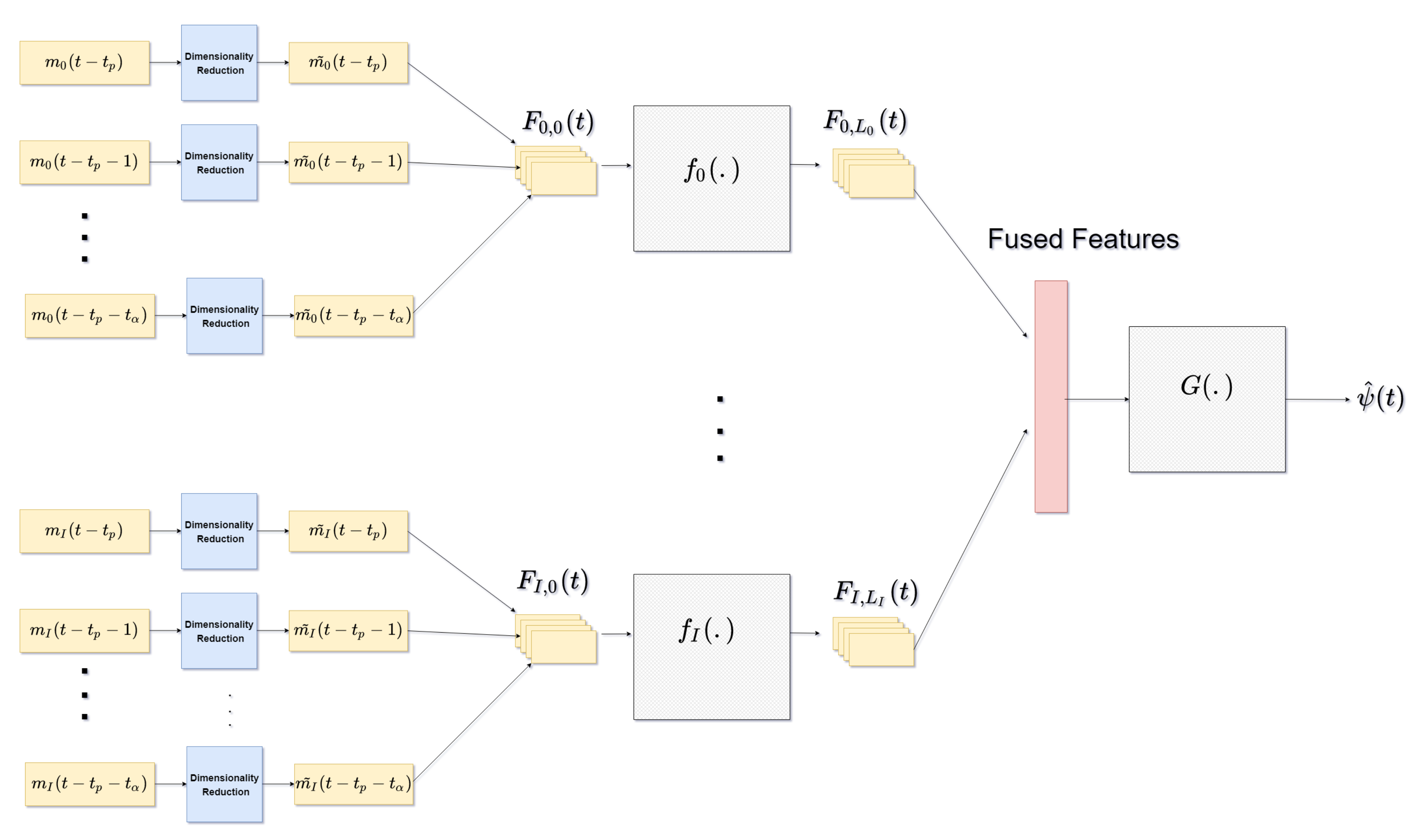
Figure 1 shows the general architecture of the model. The functions are realized by CNNs which act as localized feature extractors while which as a function accomplishing non-linear feature-level fusion, is realized by a fully connected neural network (NN). Each of the measurement modalities forms a dynamical system exhibiting non-linear spatial interactions within itself. For instance, different wind and oceanic currents interact with each other to form complex dynamic patterns. The complexity of the process we are seeking to model, is further illustrated by not only the non-linear information of each of the measurement to the global objective, but by also the non-uniformity of their respective contributions. We have modelled these self-interactions and selective weighing of modalities by feeding the modality to a separate CNN pipeline, , with no shared weights with other pipelines, and then fusing them together in later stage via the function . Separating of modalities in prior to extracting the features is justified by the fact that different modalities represent different heterogeneous physical processes.
Information in each of the modality data is tightly refined by dimensionality reduction of to get prior to proceeding to feature extraction. This is further discussed in the next subsection.
Let be the output of the CNN kernel, . In the layer of CNN pipeline, corresponds to the modality. Let there be kernels in layer . Let the size of be . We can then write
where invokes a sequential application of non-linear leaky ReLU function followed by average pooling and batch normalization. are bias terms. The input to the first layer is such that, , .
Each has such layers. The outputs of all the independent ’s are then vectorized and concatenated together to obtain:
where signifies the vectorization operator.
is then fed to a fully connected NN. The NN has weights applied at its layer m to get the output, for the neuron as,
where, is the non-linear leaky ReLU function, and are the bias terms.
The final layer has only one neuron which outputs the predicted value, .
The training is guided by the minimization of the mean squared error between and . To avoid overfitting, we also regularize the weights of the model by minimizing their L1-norm. Thus, the optimization task performed is:
where is the total number of samples in the training set and is a hyperparameter determining the relative significance of regularization in comparison to the average mean squared error.
Dimensionality Reduction/Information Extraction
The data at all locations across the globe is also not always required. For example, the weather phenomena occurring above the continental landmasses, and also in extreme northern Arctic and southern Antarctic regions may not have any significant effect on ENSO and tropical cyclone activity. We must come up with strategies to extract ’useful’ information from the raw modalities data.
We first tried to select specific patches of the global grid as input to the . The patches were selected on the basis of covariance , filtering out locations with low covariance magnitude. Richman et al. [13] used this method to make prediction on tropical hurricane count by using rank correlation maps over SST data to select attributes for their SVR based prediction model. However, in case of large prediction windows ( months), the covariance between the predictor modalities and the predictands is very low at most geographical locations. So, a better way for information extraction is in order. Singular Value Decomposition (SVD) analysis is a well proven method which generalizes eigenvalue decomposition to decompose a matrix into mutually orthogonal components. In our case, we form a predictand weighted matrix from each of the modalities global data and perform SVD analysis on it.
We perform SVD on a predictand weighted matrix from each of the modalities global data, i.e.,
where
.
Taking the product of D and is tantamount to weighting each of the global maps in at the time instant, with the value of at at the time intant t. It can be argued, that SVD of also performs a similar projection, with the exception that now we have two mutually coupled spaces. One space has temporal characteristics of with column vectors of U forming its basis vectors, while the other space has spatial characteristics of with column vectors of forming its basis vectors.
We performed this SVD analysis over each modality separately, which led to the unveiling of some interesting patterns. We observed that:
- Approximately 10–20 s-values hold above 5% relative significance. Most of these s-values have relatively similar significance.
- 50–100 s-values hold above 1% relative significance.
- No single s-value holds above 15% significance.
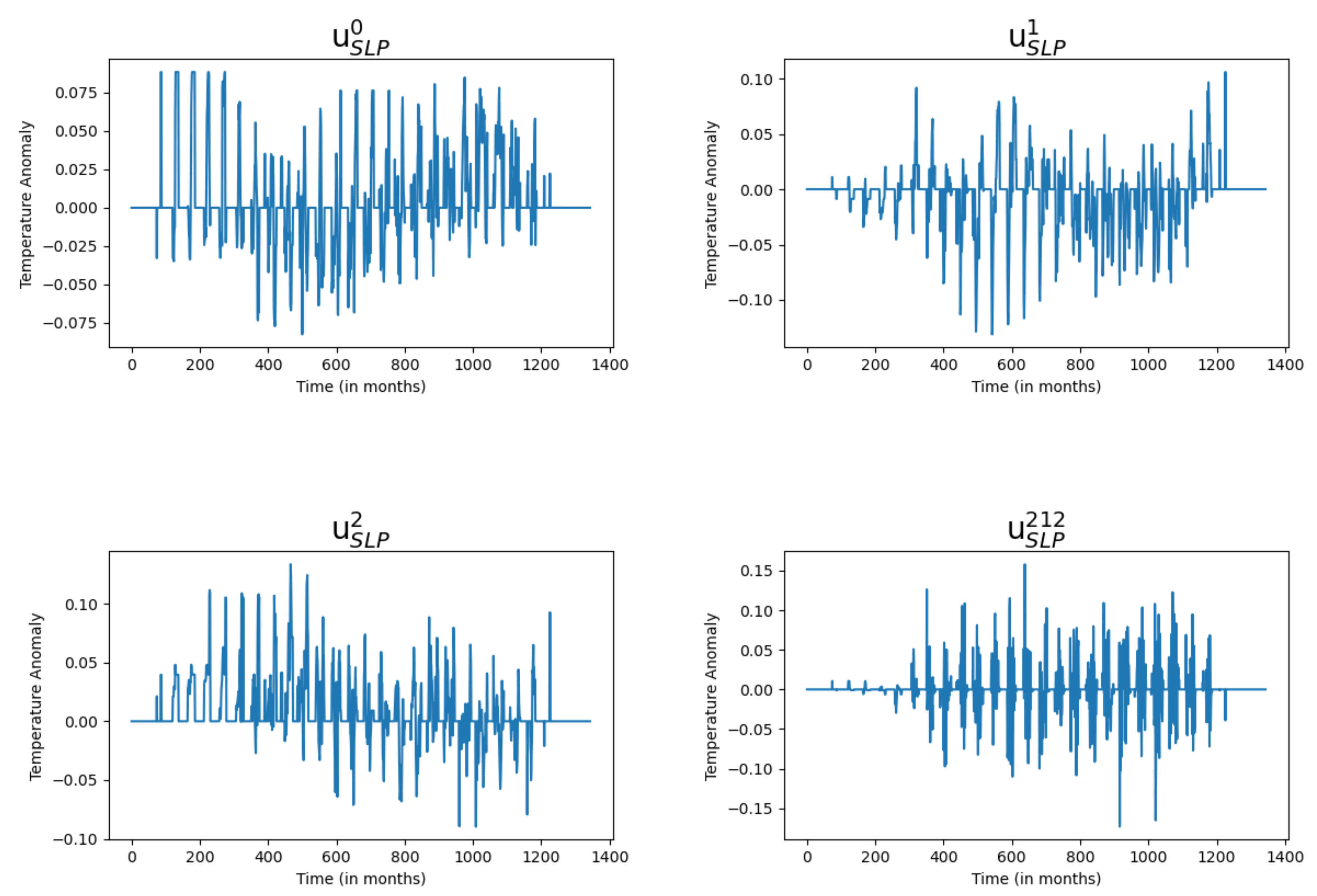
Similar trends were observed across all modalities. Figure 2 and Figure 3 show, as an example, some arbitrary U and V column vectors corresponding to NINO3.4 weighted bimonthly SLP with months. U vectors are plotted as 1-D time series. On the other hand, V vectors are reshaped into 2-D matrices of the same shape as the original SLP spatial data (i.e., ). As expected the vectors corresponding to less significant s-values are have more high frequency or noisy variations. The vectors corresponding to most significant s-values are temporally/spatially slowly varying. Physical intuition behind this pattern can be that components corresponding to more significant s-values represent spatially large-scale or temporally slowly varying environmental processes, while those corresponding to less significant s-values represent more localized phenomena. As NINO indices and ACE correspond to spatially very large and slow varying phenomena, most of the useful information is contained in components corresponding to the significant s-values.
Let the subscript subscript imply dimensionally reduced version of the matrices involved formed by taking only first r column vectors in and , and taking only first r singular values in . In our final models, we set r to 50 for the prediction of NINO indices and 10 for the prediction of ACE. Higher value of r for NINO indices in comparison to ACE was decided to account for higher temporal variation prevalent in NINO indices curves (Compare real). Reducing r any further reduced the prediction accuracy.
Further, we can get dimensionally reduced version of the original modality matrix, as,
Above operations work only when we have values readily available, which is the case with training set samples. However, when using the already trained model to do actual prediction, we would not have available at all, as this is the very value we are trying to predict. This supposed conundrum can be resolved if we observe that,
Then, we have,
Thus, once and have been calculated from the training set samples of and W, new samples of can be calculated using Equation (13). Then, we can use the row vectors of , reshaped into 2-D matrices , as input to .
7. Experiments
We used NCEP/NCAR Reanalysis Dataset [26] to gather data for above modalities. Many different data sources were assimilated together to generate the Reanalysis dataset. Sources include surface observations, upper-air balloon observations, aircraft observations, and satellite observations. An assimilated dataset has the advantage that it is available for each grid point at each time step. However, as there are multiple data sources whose quality may not be uniform throughout spatial and temporal range, accuracy may not be consistent over the whole range.
To decrease the number of computations while training the model, all the modalities were spatially interpolated to a lower common resolution of . The temporal resolution was also changed to 15 days per time sample. All modalities were then standardized, by subtracting long-term temporal mean and dividing by the standard deviation at each spatial grid-point. The temporal means and standard deviations used for standardizing are not constant throughout the temporal range (1948 to 2019) of the datasets. Instead a running window of 10 years is used. The rationale for using 10-year averages is to take into account the very long term change in environmental conditions due to global climate change. NOAA’s Climate Prediction Center uses a 30-year running mean over SST data when calculating ENSO indices [27]. We decided to use an even shorter window to better capture the effects of recent human activities on global climate change. By using a shorter window, we vary our running mean more frequently. A slowly varying mean can potentially mask information related to sample to sample variation.
Training was carried out using bimonthly data for the years ranging from 1951 to 2010. In case of ACE, only the data for the months of June to November was used, as for all other months, ACE value was almost always 0. Each consisted of 3 layers, with each layer consisting of convolution, ReLU activation average pooling and batch-normalization operations in order. As stated earlier in Section 5, there are kernels in layer of the CNN pipeline . The size of kernel is . The number of kernels in successive layers of each were 32, 64 and 128. The kernel sizes for different layers staring from first layer were , and , respectively. The fully connected part of the model had 4 layers, with the number of neurons in starting from first layer being 32,256, 5000, 500, 30 and 1.
8. Results
8.1. Prediction Accuracy
Figure 4 shows prediction results NINO3.4 index for the period of January 2012 to December 2017 from models trained using features extracted using SVD based dimensionality reduction for & 12 months. Actual training was done for bimonthly NINO3.4 index. The monthly predictions were calculated by simply averaging the two bimonthly predictions for each month. The predictions from January 2015 till June 2017 are particularly lower in case of months in comparison to the ground truth. We also observed that using a shallower network (with just 2 convolutional layers in each ) leads to a damped result. Thus using more layers results in effectively building a higher order system which is less damped. In our experiments changing model constraints like number & size of convolutional filters, number of neurons in the fully-connected layers or choosing number of singular values among myriad other things affected the over-all bias of the predictions. Increasing the depth of the CNN’s particularly decreased damping giving enough capacity to the model to capture high variations corresponding to extremely rare events. Figure 5 shows prediction for monthly NINO1 + 2 index. The general architecture is again the same as what we used for NINO3.4.
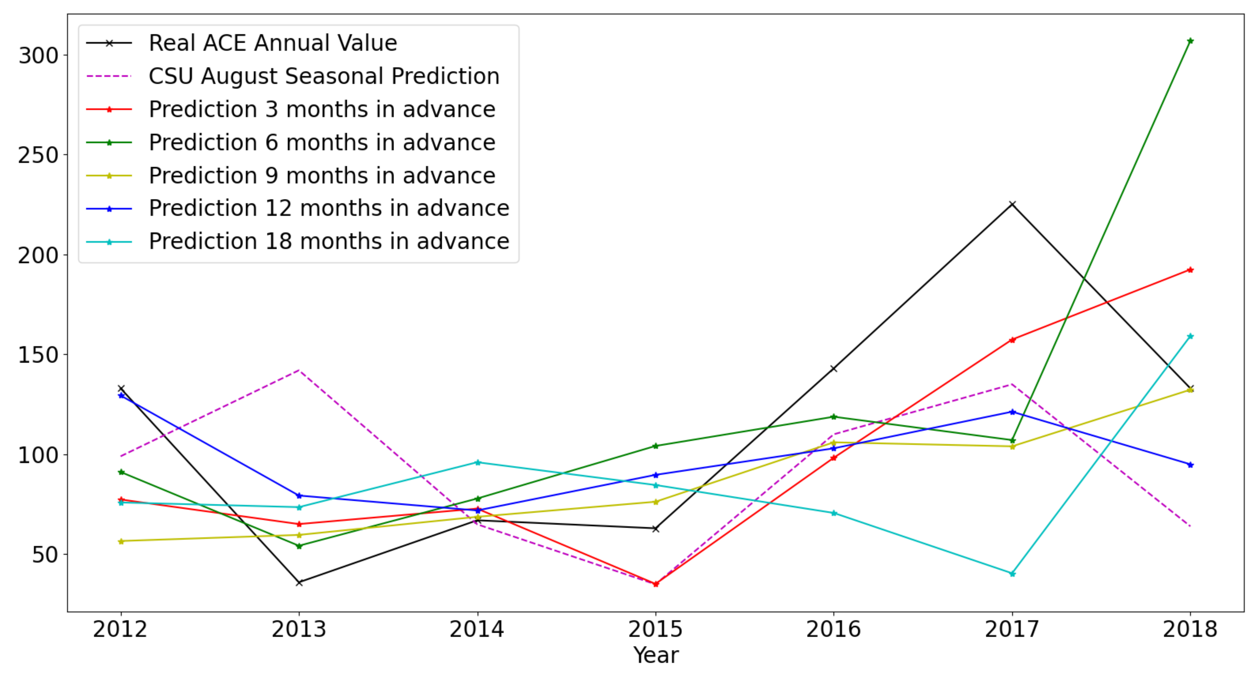
Figure 6 shows annual Atlantic ACE predictions for the period of 2012 to 2018, with prediction windows of 3, 6, 9, 12 and 18 months. Only the months of June to November are considered which correspond to the annual hurricane season. Actual training was done for bimonthly ACE. The annual ACE predictions were calculated by simply adding together all the bimonthly ACE predictions for each year. So, although the figure shows 7 sample points, the actual prediction generated 84 sample points (12 bimonthly predictions for the 6 months of June to November for each year). However, another model generating bimonthly predictions on ACE was not available to us to compare our forecasts with. Klotzbach et al. [3] from Colorado State University (CSU) have developed a model based on Poisson regression to predict annual ACE. They use certain climatological indices as predictors and make prediction for each year’s ACE by compiling data from January to August for that particular year. Hence, their prediction window is approximately 1 to 3 months. The exact climatological indices they use for prediction also change from year to year. Thus, they use a very hands-on heuristic based approach to select their input features. In comparison, our prediction models work reasonably well even with 12 months to 18 months advanced prediction without relying on heuristics-based feature selection.
Table 2 shows various performance metrics for ACE prediction efficiency calculated over years ranging from 2012 to 2018. The metrics for CSU predictions made in August for the same years range is also included. It is evident that the accuracy (based on MAE and RMSE) of our model forecasts is comparable or better than the CSU model even at 12–18 months lead time. The R2 score is consistently higher or comparable to CSU model. A significantly high correlation is evident with models trained for 3, 9, and 12 months lead time. The fourth column of the table corresponds to Mean Squared Skill Score (MSSS). MSSS is used to define the forecast skill. MSSS is the percentage improvement in mean square error over a climatology. For a forecast of a time series , it is calculated as:
where is the long-term mean of . We used 35-year mean (1984–2018) for our ACE time-series. The original climatology is the calculated ACE provided by NOAA.
Positive skill indicates that the model performs better than climatology, while a negative skill indicates that it performs worse than climatology. For 2012–2018 time duration, the forecast skill of CSU model goes negative. However, prediction with months has a higher error and poor skill score. But that is due to one extreme instance of overprediction. However, the rest of our models show significantly better skill score. For further comparison, the best skill score for the latest predictions made by TSR in [28] is also around 40%. However, this high number is for their August prediction which is just 1 month before the start of the hurricane season. For a lead time greater than 3 months their skill-score is below 20%. It is also to be noted is that the test set here is very small (just 7 time samples). But we avoided increasing our test set size at the expense of decreasing our already small training set.
8.2. Prediction Reliability
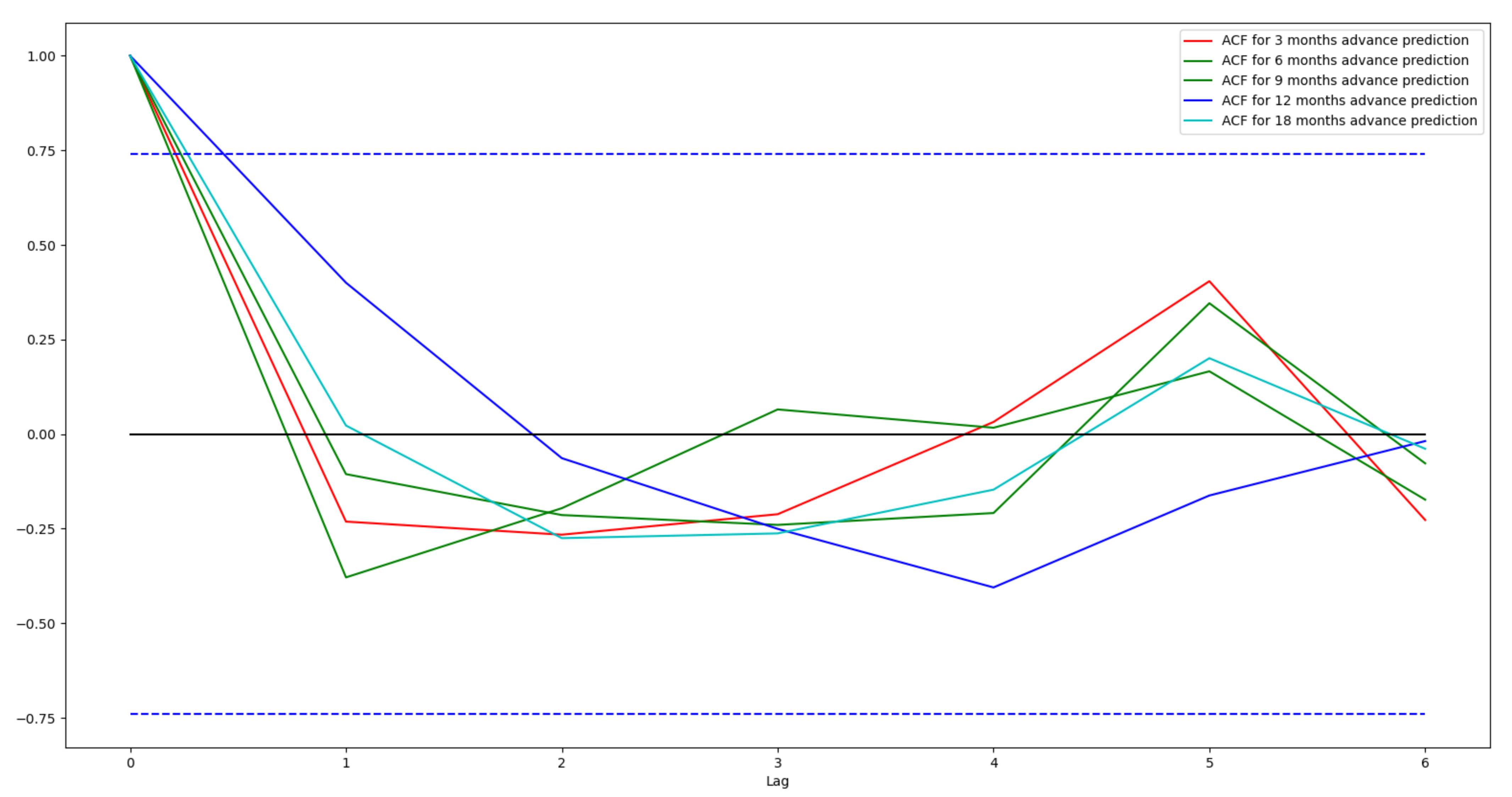
MAE, RMSE and MSSS provide metrics only on over-all prediction accuracy of a model. However, they do not provide any indication of the statistical reliability of the prediction. Ljung-Box Q test provides a measure of how the model fits the ground truth. Thus, this metric measures model reliability instead of its accuracy. If a model fits the ground truth closely, then it should be able to explain most of the trends and deterministic relationships between the dependent variable (i.e., ground truth) and various independent variables (i.e., input modalities). The residual error samples in such a case would have very little correlation among themselves and would be more like independent and identically distributed (i.i.d.) noise samples. Thus, their autocorrelation function (ACF) for non-zero lags will be very low.
If we have a time-series, of residuals with , Ljung-Box Q test assesses the null hypothesis that residuals exhibits no autocorrelation for a fixed number of lags L, against the alternative that autocorrelation is non-zero for some of the lags [29]. More specifically, the Ljung-Box Q test is defined by [30]:
where are autocorrelation coefficients at lag-k, defined as:
with . As under , all are i.i.d. with finite mean and variance, for a large n, they will be approximately iid with distribution [31]. In this case, Q would asymptotically follow a distribution with L degrees of freedom. The null hypothesis is rejected if
where is the quantile of the distribution with L degrees of freedom. is the significance level of the test. Livieris et al. [29] have demonstrated the use of Ljung-Box Q test as a reliability measure of their deep-learning model used to forecast time-series related to financial market, energy sector and cryptocurrency.
Figure 7 shows ACF plots for the residuals from various ACE prediction models with lags ranging from 0 to 6. The region between the dashed blue lines is the interval for 95% confidence that the residuals are i.i.d. with a Gaussian distribution. As can be seen for all non-zero lags the ACF plots are inside this interval thus providing acceptance to the hypothesis of i.i.d. Guassian distribution of the residuals. However, as the number of samples in the test set is low, the confidence interval is quite wide. Even then, our Ljung-Box Q statistics indicate that our predictions do fit the ground truth.
For our test set of ACE, and . Table 3 shows the Ljung-Box Q statistics calculated for variuos models and their corresponding p-values. The critical value for L = 6 at % significance is 12.59. We accept null hypothesis if Q score is less than this critical value, or p-value is higher than significance level. As can be seen p-value is always higher than a significance level of 5%. Thus, null hypothesis is accepted which demonstrates the goodness of fit of the models.
9. Conclusions
In this work, we developed a Fused-CNN architecture for the prediction of various one-dimensional indices related to hurricane activity in the Atlantic ocean. Feature level fusion provides a natural way to analyze the architecture. The model is also sufficiently simple to modify. For addition (deletion) of any modality, we can simply add (remove) the corresponding CNN pipeline. We also learned that increasing the number of layers in the CNN pipelines reduces damping of the system. Future work may explore similar architecture to make short term as well as long term predictions at a much higher spatial resolution. In other words, instead of predicting ACE for the whole of Atlantic Ocean predictions may be made for smaller patches. By increasing resolution further, we can aim to predict hurricane track patterns as well. In this case, we would have to be more surgical in our feature extraction process or increase our window of focus significantly to capture more temporal dynamics.
We achieve competitive prediction accuracy in comparison with other state of the art models, even for lead times as long as 18 months. However, the large number of significant singular values (50 for NINO indices and 10 for ACE) required in the input data makes it difficult to come up with cogent physical arguments to explain the patterns shown by the individual SVD components. All s-values are below 15% in relative significance. Hence, to keep enough relevant information while filtering out noise, we had to keep 10 to 50 s-values for various models. Had the number of significant s-values been below 10 (for instance 2 or 3), we might have been able to associate the variations seen in the corresponding v-vectors with some specific weather patterns.
It is also to be noted that while doing SVD analysis, we have been separately looking at each predictand weighted modality. We are still unable to observe the effect of one modality/predictor over another modality/predictor. Our future goal is to enhance our feature extraction process to include these interdependencies. Additionally, although 84 data points were used in our bimonthly test dataset, a comparison with other models could be carried out only at annual time scale due to the unavailability of the bimonthly forecasts from other models used for comparison. More robust model inter-comparisons should be made in the future when longer forecast and validation datasets become readily available.
Author Contributions
Conceptualization, L.X. and H.K. Methodology, H.K., L.X., T.A., S.R.; Software, T.A., S.R.; Validation, T.A., H.K., X.S. and L.X.; Formal Analysis, T.A., H.K., L.X.; Investigation, T.A., H.K., L.X.; Resources, L.X., H.K.; Data Curation, X.S.; Writing—Original Draft Preparation, T.A.; Writing—Review & Editing, L.X., H.K., S.R.; Visualization, T.A.; Supervision, H.K., L.X.; Project Administration, L.X.; Funding Acquisition, L.X. All authors have read and agreed to the published version of the manuscript.
Funding
This study is funded by the National Science Foundation’s Center for Accelerated Real-Time Analytics (CARTA) through award#2020–2696. This work is also in large part funded by the generous support of ARO grant W911NF1910202.
Data Availability Statement
Datasets used in this research are available at: https://tinyurl.com/y6lfnqzr (accessed on 2 April 2021).
Acknowledgments
We appreciate the support of Rada Chirkova and David Wright at the NC State University site of the NSF CARTA center during the course of this study.
Conflicts of Interest
The authors declare no conflict of interest.
References
- Bauer, P.; Thorpe, A.; Brunet, G. The quiet revolution of numerical weather prediction. Nature 2015, 525, 47. [Google Scholar] [CrossRef] [PubMed]
- Blake, E.S.; Gray, W.M. Prediction of August Atlantic basin hurricane activity. Weather Forecast. 2004, 19, 1044–1060. [Google Scholar] [CrossRef] [Green Version]
- Klotzbach, P.; Blake, E.; Camp, J.; Caron, L.P.; Chan, J.C.; Kang, N.Y.; Kuleshov, Y.; Lee, S.M.; Murakami, H.; Saunders, M.; et al. Seasonal Tropical Cyclone Forecasting. Trop. Cyclone Res. Rev. 2014, 8, 134–149. [Google Scholar] [CrossRef]
- Camargo, S.J.; Barnston, A.G.; Klotzbach, P.J.; Landsea, C.W. Seasonal tropical cyclone forecasts. WMO Bull. 2007, 56, 297–309. [Google Scholar]
- Hughes, G.F. On the mean accuracy of statistical pattern recognizers. IEEE Trans. Inf. Theory 1968, 14, 55–63. [Google Scholar] [CrossRef] [Green Version]
- Roheda, S.; Krim, H.; Riggan, B.S. Robust Multi-Modal Sensor Fusion: An Adversarial Approach. IEEE Sens. J. 2021, 21, 1885–1896. [Google Scholar] [CrossRef]
- Roheda, S.; Krim, H.; Luo, Z.; Wu, T. Decision Level Fusion: An Event Driven Approach. In Proceedings of the 2018 26th European Signal Processing Conference (EUSIPCO), Rome, Italy, 3–7 September 2018; pp. 2598–2602. [Google Scholar]
- Saunders, M.A.; Klotzbach, P.J.; Lea, A.S.R.; Schreck, C.J.; Bell, M.M. Quantifying the probability and causes of the surprisingly active 2018 North Atlantic hurricane season. Earth Space Sci. 2020, 7, e2019EA000852. [Google Scholar] [CrossRef] [Green Version]
- Davis, K.; Zeng, X.; Ritchie, E.A. A New Statistical Model for Predicting Seasonal North Atlantic Hurricane Activity. Weather. Forecast. 2015, 30, 730–741. [Google Scholar] [CrossRef]
- Kozar, M.E.; Mann, M.E.; Camargo, S.J.; Kossin, J.P.; Evans, J.L. Stratified statistical models of North Atlantic basin-wide and regional tropical cyclone counts. J. Geophys. Res. Atmos. 2012, 117, D18. [Google Scholar] [CrossRef] [Green Version]
- Keith, E.; Xie, L. Predicting Atlantic Tropical Cyclone Seasonal Activity in April. Weather. Forecast. 2009, 24, 436–455. [Google Scholar] [CrossRef]
- Alemany, S.; Beltran, J.; Perez, A.; Ganzfried, S. Predicting Hurricane Trajectories Using a Recurrent Neural Network. Proc. Aaai Conf. Artif. Intell. 2019, 33, 468–475. [Google Scholar] [CrossRef] [Green Version]
- Richman, M.B.; Leslie, L.M.; Ramsay, H.A.; Klotzbach, P.J. Reducing tropical cyclone prediction errors using machine learning approaches. Procedia Comput. Sci. 2017, 114, 314–323. [Google Scholar] [CrossRef]
- LeCun, Y.; Bengio, Y.; Hinton, G. Deep learning. Nature 2015, 521, 436. [Google Scholar] [CrossRef]
- Ledig, C.; Theis, L.; Huszár, F.; Caballero, J.; Cunningham, A.; Acosta, A.; Aitken, A.; Tejani, A.; Totz, J.; Wang, Z.; et al. Photo-realistic single image super-resolution using a generative adversarial network. In Proceedings of the IEEE Conference on Computer Vision and Pattern Recognition (CVPR), Honolulu, HI, USA, 21–26 July 2017; IEEE: New York, NY, USA, 2017. [Google Scholar]
- Tran, K.; Panahi, A.; Adiga, A.; Sakla, W.; Krim, H. Nonlinear Multi-scale Super-resolution Using Deep Learning. ICASSP 2019, 2019, 3182–3186. [Google Scholar]
- Yang, D.; Sun, J. Bm3d-net: A convolutional neural network for transformdomain collaborative filtering. IEEE Signal Process. Lett. 2018, 25, 55–59. [Google Scholar] [CrossRef]
- Ham, Y.G.; Kim, J.H.; Luo, J.J. Deep learning for multi-year ENSO forecasts. Nature 2019, 573, 568. [Google Scholar] [CrossRef]
- Merrill, R.T. Environmental influences on hurricane intensification. J. Atmos. Sci. 1988, 45, 1678–1687. [Google Scholar] [CrossRef] [Green Version]
- Shaman, J.; Esbensen, S.K.; Maloney, E.D. The dynamics of the ENSO—Atlantic hurricane teleconnection: ENSO-related changes to the North African—Asian Jet affect Atlantic basin tropical cyclogenesis. J. Clim. 2009, 22, 2458–2482. [Google Scholar] [CrossRef] [Green Version]
- Klotzbach, P.J. El Niño—Southern Oscillation’s Impact on Atlantic Basin Hurricanes and U.S. Landfalls. J. Clim. 2011, 24, 1252–1263. [Google Scholar] [CrossRef]
- Trenberth, K.E. The Definition of El Nino. Bull. Am. Meteorol. Soc. 1997, 78, 2771–2777. [Google Scholar] [CrossRef] [Green Version]
- Trenberth, K.; David, E.; Stepaniak, P. Indices of El Niño evolution. J. Clim. 2001, 14, 1697–1701. [Google Scholar] [CrossRef] [Green Version]
- Sun, C.; Shrivastava, A.; Singh, S.; Gupta, A. Revisiting Unreasonable Effectiveness of Data in Deep Learning Era. In Proceedings of the 2017 IEEE International Conference on Computer Vision (ICCV), Venice, Italy, 22–29 October 2017; pp. 843–852. [Google Scholar] [CrossRef] [Green Version]
- Gray, W.M.; Landsea, C.W.; Sea, C.W.; Mielke, P.W.; Berry, K.J. Forecast of Atlantic Seasonal Hurricane Activity for 1988; Colorado State University: Fort Collins, CO, USA, 1988; pp. 13–14. [Google Scholar]
- Kalnay, E.; Kanamitsu, M.; Kistler, R.; Collins, W.; Deaven, D.; Gandin, L.; Iredell, M.; Saha, S.; White, G.; Woollen, J.; et al. The NCEP/NCAR 40-year reanalysis project. Bull. Am. Meteorol. Soc. 1996, 77, 437–470. [Google Scholar] [CrossRef] [Green Version]
- Lindsey, R. In Watching for El Niño and La Niña, NOAA Adapts to Global Warming. Underrstanding Climate, NOAA Climate.gov. Available online: https://www.climate.gov/news-features/understanding-climate/watching-el-niño-and-la-niña-noaa-adapts-global-warming (accessed on 2 April 2021).
- Saunders, M.A.; Lea, A. Extended Range Forecast for Atlantic Hurricane Activity in 2021. 2020. Available online: Tropicalstormrisk.com (accessed on 2 April 2021).
- Livieris, I.E.; Stavroyiannis, S.; Pintelas, E.; Pintelas, P. A novel validation framework to enhance deep learning models in time-series forecasting. Neural Comput. Appl. 2020, 32, 17149–17167. [Google Scholar] [CrossRef]
- Ljung, G.M.; Box, G.E.P. On a measure of lack of fit in time series models. Biometrika 1978, 65, 297–303. [Google Scholar] [CrossRef]
- Brockwell, P.J.; Davis, R.A. Time Series: Theory and Methods, 2nd ed.; Springer: New York, NY, USA, 1991. [Google Scholar]
Figure 1.
Architecture showing feature level fusion.

Figure 2.
Column vectors, , , and for . x-axis is the index value and y-axis is the amplitude. The vectors are plotted as 1-D time series.The D matrix is formed by months).
Figure 2.
Column vectors, , , and for . x-axis is the index value and y-axis is the amplitude. The vectors are plotted as 1-D time series.The D matrix is formed by months).

Figure 3.
Reshaped column vectors (in clockwise order starting from upper left), , , and for . The vectors were reshaped to 2-D matrices with same shape as the original SLP map (). The W matrix is formed by months).
Figure 3.
Reshaped column vectors (in clockwise order starting from upper left), , , and for . The vectors were reshaped to 2-D matrices with same shape as the original SLP map (). The W matrix is formed by months).
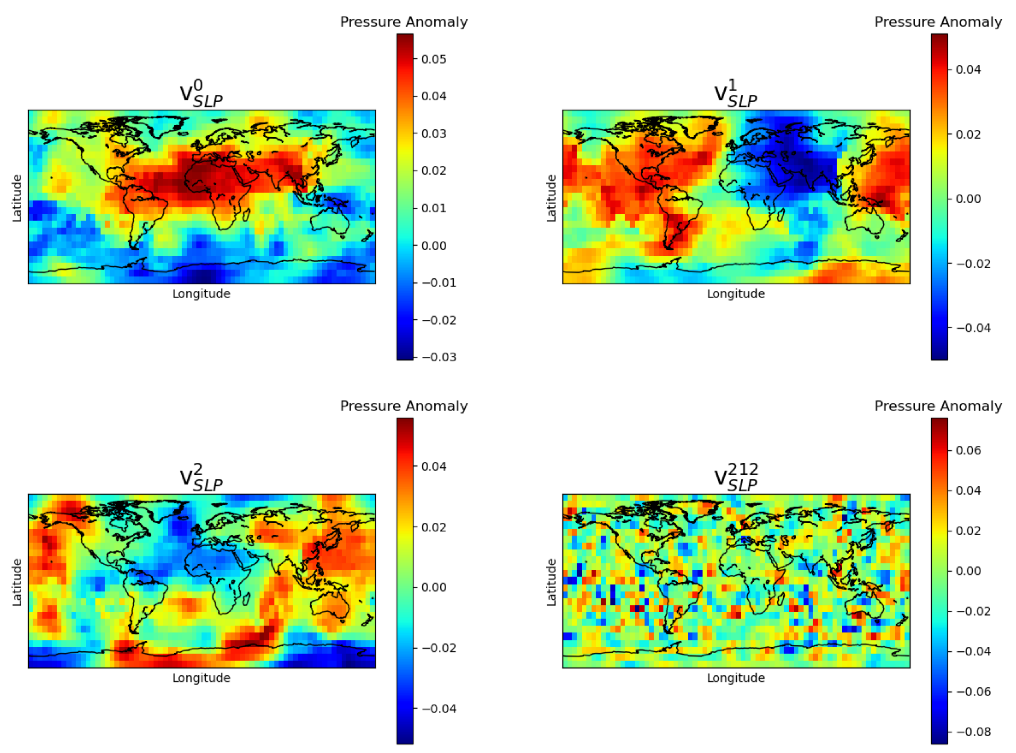
Figure 4.
Monthly NINO3.4 predictions (January 2012 to December 2017) using SVD based dimensionality reduction compared with the original NINO3.4 index (black curve). x-axis is months starting from January, 2012.
Figure 4.
Monthly NINO3.4 predictions (January 2012 to December 2017) using SVD based dimensionality reduction compared with the original NINO3.4 index (black curve). x-axis is months starting from January, 2012.
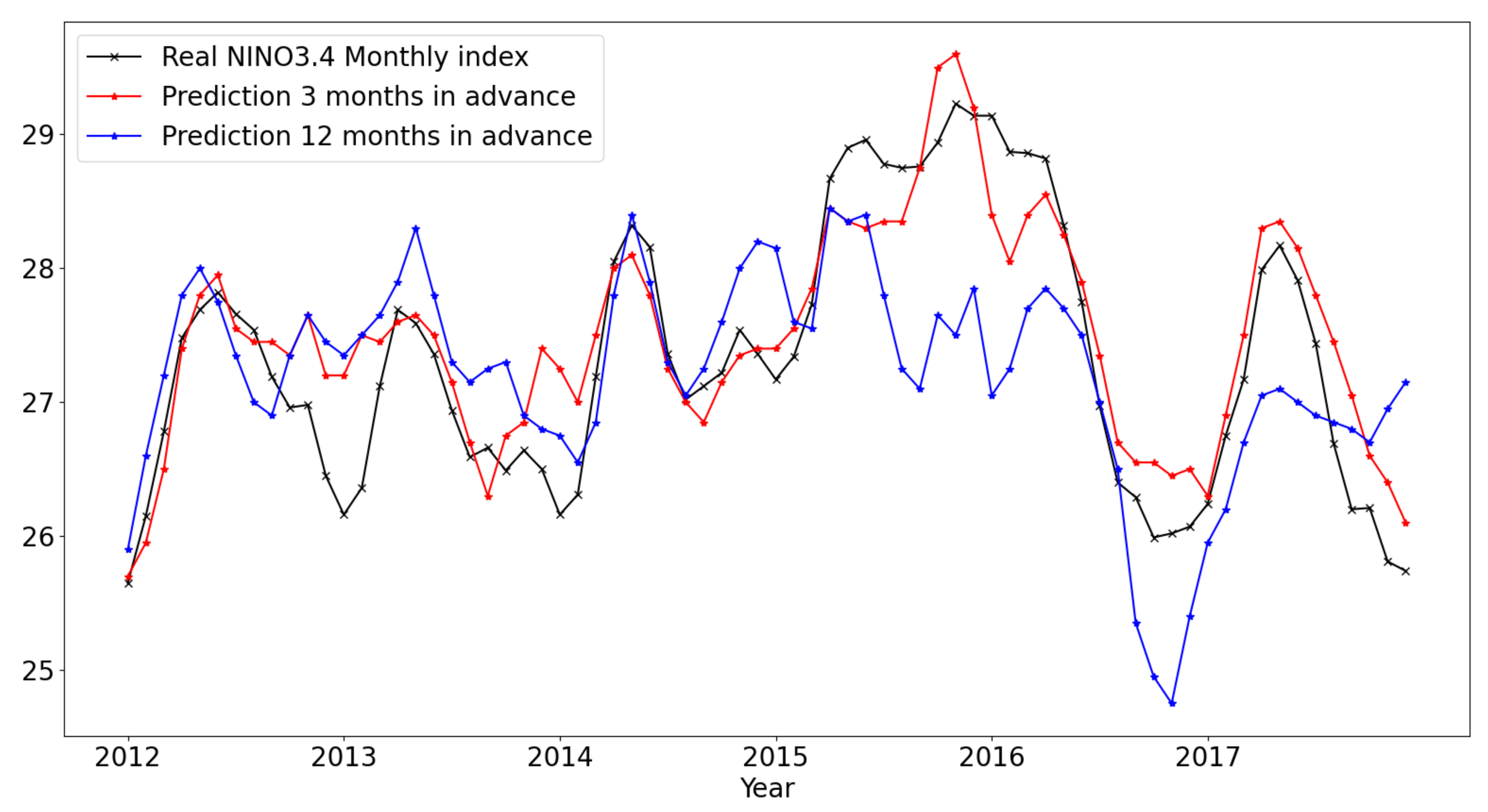
Figure 5.
Monthly NINO1.2 predictions (January 2012 to December 2017) using SVD based dimensionality reduction compared with the original NINO1.2 index (black curve). x-axis is months starting from January, 2012.
Figure 5.
Monthly NINO1.2 predictions (January 2012 to December 2017) using SVD based dimensionality reduction compared with the original NINO1.2 index (black curve). x-axis is months starting from January, 2012.

Figure 6.
Annual Atlantic ACE predictions (2012 to 2018) using SVD based dimensionality reductions compared with the Poisson regression based seasonal predictions done by Colorado State University in August each year (dashed blue curve) and the original ACE curve (black curve).
Figure 6.
Annual Atlantic ACE predictions (2012 to 2018) using SVD based dimensionality reductions compared with the Poisson regression based seasonal predictions done by Colorado State University in August each year (dashed blue curve) and the original ACE curve (black curve).

Figure 7.
Autocorrelation function plots for residuals from ACE prediction models. Dashed blue lines show intervals for 95% confidence.
Figure 7.
Autocorrelation function plots for residuals from ACE prediction models. Dashed blue lines show intervals for 95% confidence.


Table 1.
Descriptions of data used in the prediction model.
| Model | Role in the Model | Spatial Resolution | Original Temporal Resolution | Temporal Resolution Used in the Model | Data Source |
|---|---|---|---|---|---|
| NINO3.4 () | Predictand | NA | Monthly | Bimonthly | NOAA |
| NINO1 + 2 () | Predictand | NA | Monthly | Bimonthly | NOAA |
| ACE () | Predictand | NA | Annual | Bimonthly | HURDAT2 |
| Sea Level Pressure () | Predictor | 4 times Daily | Bimonthly | NCEP-NCAR | |
| Sea Surface Temperature () | Predictor | 4 times Daily | Bimonthly | NCEP-NCAR | |
| Zonal Wind Speed at 850 mb () | Predictor | 4 times Daily | Bimonthly | NCEP-NCAR | |
| Meridional Wind Speed at 850 mb () | Predictor | 4 times Daily | Bimonthly | NCEP-NCAR | |
| Zonal Wind Speed at 200 mb () | Predictor | 4 times Daily | Bimonthly | NCEP-NCAR | |
| Meridional Wind Speed at 200 mb () | Predictor | 4 times Daily | Bimonthly | NCEP-NCAR | |
| Relative Humidity at 700 mb () | Predictor | 4 times Daily | Bimonthly | NCEP-NCAR |
Table 2.
ACE pediction efficiency metrics for different prediction windows compared with CSU seasonal predictions made in August.
Table 2.
ACE pediction efficiency metrics for different prediction windows compared with CSU seasonal predictions made in August.
| Model | MAE | RMSE | R2 | MSSS |
|---|---|---|---|---|
| CSU August Prediction | 51.71 | 62.26 | 0.0719 | −9.48% |
| Fused CNN with months | 41.44 | 46.05 | 0.4571 | 40.09% |
| Fused CNN with months | 61.15 | 83.31 | 0.0800 | −96.04% |
| Fused CNN with months | 39.11 | 56.80 | 0.3079 | 8.87% |
| Fused CNN with months | 37.19 | 48.45 | 0.5779 | 33.70% |
| Fused CNN with months | 61.19 | 81.00 | 0.0656 | −85.35% |
Table 3.
Prediction reliability metrics over the Test set (2012–2018) for different prediction windows with significance level of 0.05.
Table 3.
Prediction reliability metrics over the Test set (2012–2018) for different prediction windows with significance level of 0.05.
| Model | Ljung Box Q Score | p-Value | Null |
|---|---|---|---|
| CSU August Prediction | 5.45 | 0.49 | Accepted |
| Fused CNN with months | 10.57 | 0.1 | Accepted |
| Fused CNN with months | 4.82 | 0.57 | Accepted |
| Fused CNN with months | 6.66 | 0.35 | Accepted |
| Fused CNN with months | 7.02 | 0.32 | Accepted |
| Fused CNN with months | 3.86 | 0.7 | Accepted |
Publisher’s Note: MDPI stays neutral with regard to jurisdictional claims in published maps and institutional affiliations. |
© 2021 by the authors. Licensee MDPI, Basel, Switzerland. This article is an open access article distributed under the terms and conditions of the Creative Commons Attribution (CC BY) license (https://creativecommons.org/licenses/by/4.0/).
Share and Cite
MDPI and ACS Style
Asthana, T.; Krim, H.; Sun, X.; Roheda, S.; Xie, L. Atlantic Hurricane Activity Prediction: A Machine Learning Approach. Atmosphere 2021, 12, 455. https://0-doi-org.brum.beds.ac.uk/10.3390/atmos12040455
AMA Style
Asthana T, Krim H, Sun X, Roheda S, Xie L. Atlantic Hurricane Activity Prediction: A Machine Learning Approach. Atmosphere. 2021; 12(4):455. https://0-doi-org.brum.beds.ac.uk/10.3390/atmos12040455
Chicago/Turabian StyleAsthana, Tanmay, Hamid Krim, Xia Sun, Siddharth Roheda, and Lian Xie. 2021. "Atlantic Hurricane Activity Prediction: A Machine Learning Approach" Atmosphere 12, no. 4: 455. https://0-doi-org.brum.beds.ac.uk/10.3390/atmos12040455
Note that from the first issue of 2016, this journal uses article numbers instead of page numbers. See further details here.