Article

Aerosol and Cloud Detection Using Machine Learning Algorithms and Space-Based Lidar Data

1
NASA Goddard Space Flight Center, Greenbelt, MD 20771, USA
2
Science Systems and Applications, Inc., Lanham, MD 20706, USA
3
Earth System Science Interdisciplinary Center, University of Maryland, College Park, MD 20740, USA
4
Department of Climate and Space Sciences and Engineering, University of Michigan, Ann Arbor, MI 48109, USA
*
Author to whom correspondence should be addressed.
Submission received: 26 March 2021 / Revised: 13 April 2021 / Accepted: 23 April 2021 / Published: 7 May 2021
(This article belongs to the Special Issue Lidar Remote Sensing Techniques for Atmospheric Aerosols)

Abstract

:
Clouds and aerosols play a significant role in determining the overall atmospheric radiation budget, yet remain a key uncertainty in understanding and predicting the future climate system. In addition to their impact on the Earth’s climate system, aerosols from volcanic eruptions, wildfires, man-made pollution events and dust storms are hazardous to aviation safety and human health. Space-based lidar systems provide critical information about the vertical distributions of clouds and aerosols that greatly improve our understanding of the climate system. However, daytime data from backscatter lidars, such as the Cloud-Aerosol Transport System (CATS) on the International Space Station (ISS), must be averaged during science processing at the expense of spatial resolution to obtain sufficient signal-to-noise ratio (SNR) for accurately detecting atmospheric features. For example, 50% of all atmospheric features reported in daytime operational CATS data products require averaging to 60 km for detection. Furthermore, the single-wavelength nature of the CATS primary operation mode makes accurately typing these features challenging in complex scenes. This paper presents machine learning (ML) techniques that, when applied to CATS data, (1) increased the 1064 nm SNR by 75%, (2) increased the number of layers detected (any resolution) by 30%, and (3) enabled detection of 40% more atmospheric features during daytime operations at a horizontal resolution of 5 km compared to the 60 km horizontal resolution often required for daytime CATS operational data products. A Convolutional Neural Network (CNN) trained using CATS standard data products also demonstrated the potential for improved cloud-aerosol discrimination compared to the operational CATS algorithms for cloud edges and complex near-surface scenes during daytime.

1. Introduction

Atmospheric features such as clouds and aerosols play an important role in Earth’s climate system, air quality and hydrological cycle, with a magnitude that is heavily dependent on the atmospheric feature’s height, thickness and type. Liquid water clouds near the Earth’s surface tend to reflect incoming sunlight, cooling Earth’s surface [1,2]. However, ice clouds in the upper troposphere absorb heat emitted from the surface and re-radiate it back down, warming Earth’s surface [3,4,5]. Aerosol particles include windblown dust from deserts, smoke from wildfires, sulfurous particles from volcanic eruptions, and particles produced by fossil fuel combustion. Depending upon their size, composition, and location within the atmosphere, aerosols either cool or warm the surface [6,7]. In general, dark-colored aerosols, such as black carbon from fossil fuel combustion, absorb radiation, heating Earth’s atmosphere, while bright-colored aerosols, such as sulfates from volcanic eruptions, reflect radiation, acting to cool Earth’s atmosphere [8,9]. Near the Earth’s surface, aerosol particles are pollutants that exacerbate poor air quality conditions contributing to an annual death toll of greater than 3 million people globally [10].
Lidar measurements provide accurate vertically resolved information about clouds and aerosols, including multi-layer scenes where passive sensors are challenged and at night, when passive sensors are unable to measure cloud and aerosol properties. Airborne lidar measurements, such as those from the Cloud Physics Lidar (CPL), play a vital role in field campaign studies of clouds and aerosols [11,12]. Since 2006, the Cloud-Aerosol Lidar with Orthogonal Polarization (CALIOP) onboard the Cloud-Aerosol Lidar and Infrared Pathfinder Satellite Observation (CALIPSO) satellite has provided vertical profiles of clouds and aerosols from space with global coverage that are essential to studies of the Earth’s climate system [13]. Fundamental measurements of attenuated total backscatter and volume depolarization ratio from these instruments are used to derive “vertical feature mask” cloud and aerosol products, including layer top/base heights, layer geometrical thickness, aerosol type, and cloud phase. The CALIPSO vertical feature mask data products have been utilized in numerous studies of clouds [14,15,16,17,18] and aerosols [19,20,21,22].
The Cloud-Aerosol Transport System (CATS) was a backscatter lidar employing photon counting detection and two high-repetition rate lasers that operated at 532 and 1064 nm [23]. Launched to the International Space Station (ISS) on 10 January 2015, CATS was first operated on 5 February 2015. CATS generated over 200 billion laser pulses during 33 months of on-orbit operation. The CATS instrument was intended to demonstrate new in-space technologies for future Earth Science missions while also providing valuable science data (e.g., vertical profiles of clouds and aerosols). The precessing ISS orbit (∼415 km altitude, 51.8 inclination) enabled CATS to measure clouds and aerosols at a different local time each overpass, observing a full diurnal cycle every ∼60 days. Additionally, the orbit inclination enabled CATS observations between 51 N and 51 S at higher frequencies than sun-synchronous orbiting sensors, making it an intriguing complement to the CALIPSO mission.
While CATS had two operational modes [24], it operated primarily in Mode 7.2, creating a dataset that spans from 25 March 2015 to 29 October 2017 and is the focus of all analysis in this paper. The CATS Level 1 (L1) and Level 2 (L2) data products are very similar to those provided by the CALIPSO mission. Similar to CALIPSO, CATS utilizes meteorological reanalyses from the NASA Goddard Earth Observing System Modern-Era Retrospective Analysis for Research and Applications, Version 2 (MERRA-2) [25] to determine the Rayleigh signal, but also to aid in cloud-aerosol discrimination as described in Section 2.2. The principal parameters of the CATS L1 product, which have resolutions of 350 m horizontal and 60 m vertical, are the attenuated total backscatter (ATB) and attenuated perpendicular backscatter (APB) coefficients, units of km 1 sr 1 , at both 532 nm and 1064 nm wavelengths. Yorks et al. (2016) [24] provides an overview of the CATS L1 data products and processing algorithms.
The final version of the CATS L1 and L2 data products was released in December 2018 (V3-01). These CATS data products enable the science community to investigate cloud and aerosol diurnal variability [26,27,28,29], impacts of clouds and aerosols on the climate system [30,31], as well as accurately monitor and model aerosol plumes [32,33,34]. This paper describes the CATS L2 operational atmospheric layer detection and cloud-aerosol discrimination data processing algorithms, as well as the strengths and limitations of these algorithms in Section 2. CATS daytime signals are degraded by noise from solar background light. The signal-to-noise ratio (SNR), a metric used to determine the accuracy that a lidar can measure backscatter, is lower during daytime than at night for CATS [35]. Historically, the primary way to improve the SNR of any space-based lidar instrument is to average the data onboard or during science data processing at the cost of horizontal resolution. In this paper we describe ML algorithms developed to both reduce noise in the daytime CATS data and more accurately predict cloud and aerosol features at finer horizontal resolutions in Section 3. We present initial results using the ML methods and compare the results of the ML techniques to the traditional operational CATS data products in Section 4.

2. CATS Level 2 Operational Data Products and Algorithms

The CATS L2 operational (L2O) layer detection and cloud-aerosol discrimination (CAD) data processing algorithms rely heavily on heritage from existing airborne and space-based lidar systems, such as CPL and CALIOP. The data products generated from the CATS measurements are produced according to a protocol that is similar to that established by NASA’s Earth Observing System (EOS). The CATS L2 data products are geophysical parameters derived from L1 data that can be separated into two categories: (1) the vertical feature mask (VFM) that includes variables such as the layer top and base, feature type, cloud phase, aerosol type, and (2) optical properties such as vertical profiles of particle extinction and backscatter coefficients, as well as layer-integrated parameters (i.e., lidar ratio, optical depth). This paper focuses on the CATS VFM data products and algorithms. The CATS L2 data products were intentionally designed to be similar to the CALIOP L2 data products, so users of space-based lidar data can seamlessly use data from both instruments. While the CATS operational processing algorithms have heritage from CALIPSO, fundamental differences between CATS and CALIPSO, such as the single-wavelength nature of the CATS M7.2 data, necessitated the development of new independent operational algorithms.
Figure 1 shows an example of the CATS operational vertical feature mask products on 24 August 2015 in which CATS flew over the west coast of Africa. The 1064 nm attenuated total backscatter (a) shows the vertical locations of the atmospheric features. The volume depolarization ratio at 1064 nm (b) shows where non-spherical particles, such as ice crystals and dust particles, are observed. These two variables, along with other properties such as layer heights, layer thickness and layer temperatures provide the basis for identifying the feature type (c). In this case CATS observed marine aerosols, dust, ice clouds, liquid water clouds, and smoke along the west coast of Africa. More details on the algorithms for producing both these CATS L2 vertical feature mask products are provided below.
There are 2 types of CATS L2O data products; (1) a merged cloud and aerosol layer product and (2) a merged cloud and aerosol profile product, both at 5 km horizontal resolutions. These products include both VFM variables shown in Table 1, as well as optical properties (optical depth, extinction coefficient, ice water content, etc.). The CATS L2O data products are different than those provided by CALIOP in that: (1) they are provided at a single resolution (not multiple products for multiple resolutions), (2) the VFM is within the same data file as the optical properties, and (3) cloud and aerosol profile products are combined into the same file.
The CATS L2O data products are produced using novel operational CATS L2 algorithms. The CATS L2O vertical feature mask algorithms were designed based on CPL and CALIOP algorithms, the performance of CATS L1B data products, and differences in the CATS instrument design compared to CPL and CALIOP. The new CATS V3 L1B data products include upgrades since the Yorks et al. (2016) [24] paper such as an added ATB uncertainty parameter, adjustments to geolocation algorithms, as well as improvements in backscatter and depolarization calibrations [35]. The primary difference between CATS and CALIOP data products, other than orbital differences, is the performance and capabilities of the two wavelengths.
CALIOP has lower uncertainties and minimum detectable backscatter (MDB, the lowest ATB that a feature can be accurately distinguished) at 532 nm than at 1064 nm. The CATS nighttime 1064 nm ATB is robust with low MDB compared to both CALIOP and CATS Mode 7.1 [24]. In addition, CATS measures volume depolarization ratio using the 1064 nm wavelength, whereas CALIOP measures volume depolarization ratio using 532 nm. Thus, the 1064 nm data is utilized heavily in the CATS L2O vertical feature mask algorithms and for any analysis that is wavelength-independent (i.e., layer detection, relative backscatter intensity). The CATS L2O layer detection and CAD algorithms are outlined in the subsections to follow.

2.1. CATS Operational Layer Detection Algorithm

The CATS L2O layer detection is performed following the methodology described in Vaughan et al. (2009) [36] and the CALIOP Algorithm Theoretical Basis Document [37,38], but applied to 1064 nm. It is a threshold-based layer detection method that uses the 1064 nm attenuated scattering ratio (attenuated total backscatter divided by the attenuated molecular backscatter). A threshold for each profile is calculated from range-variant and range-invariant sources of noise. Figure 2 shows the layer detection results from 24 August 2015 off the western coast of Africa (around 3 latitude and −4 longitude, red line in Figure 1). When the 1064 nm attenuated scattering ratio (black) is greater than the threshold profile (red), a layer is detected. In this case, four distinct layers (pink, brown, teal, and blue colors) were detected at a horizontal resolution of 5 km by the CATS L2O layer detection algorithm.
There are four primary differences between the CALIOP and CATS L2O layer detection algorithms, which are:
  • The CATS L2O algorithm uses the 1064 nm attenuated scattering ratio, unlike the CALIOP algorithm that uses 532 nm.
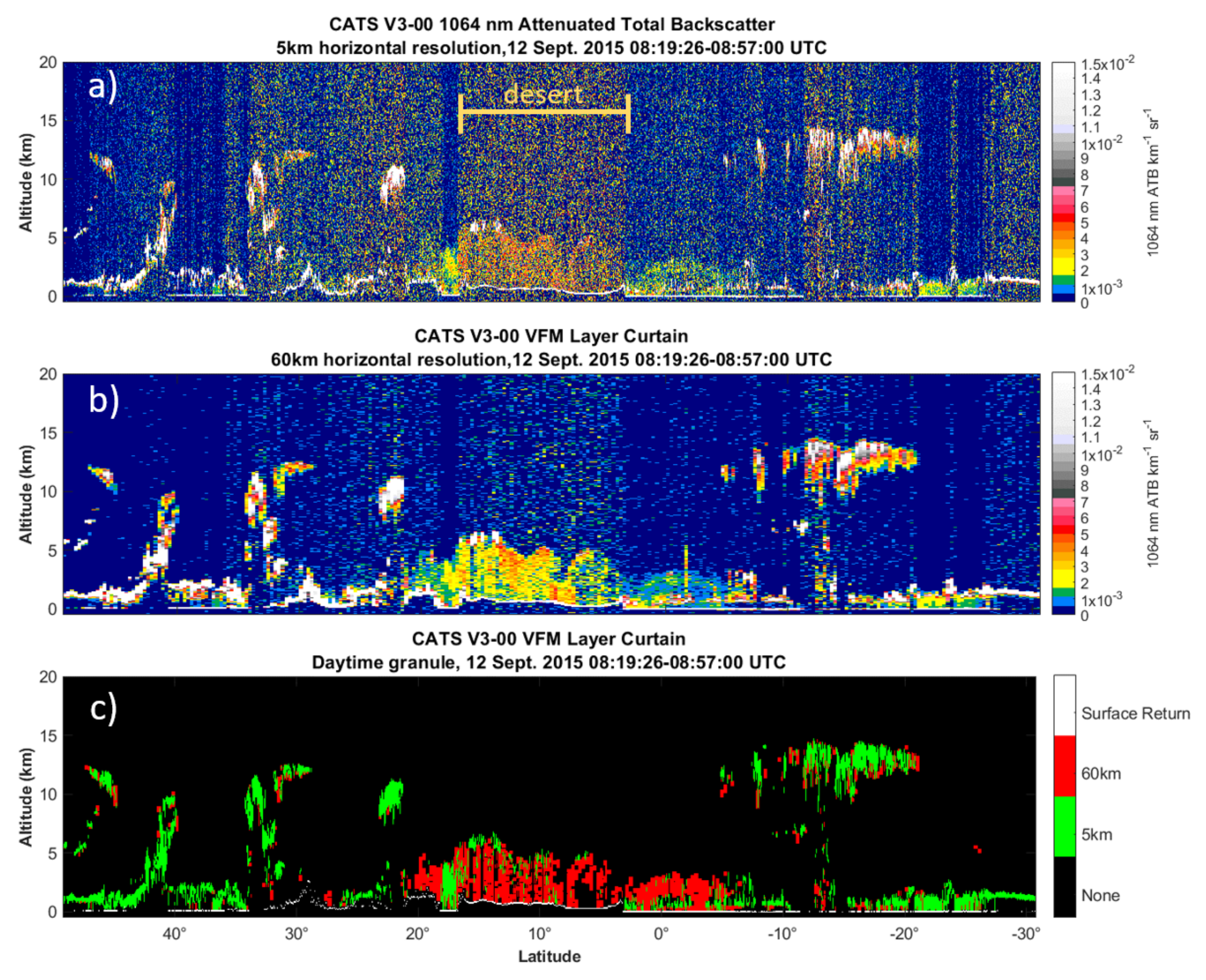
  • The CATS L2O data is averaged to only two horizontal resolutions (5 and 60 km) instead of the 5 resolutions CALIOP uses.
  • The CATS layer detection includes an algorithm to detect clouds embedded in aerosols.
  • The CATS layer detection algorithm also utilizes depolarization to create layer boundaries.
For CATS, the layer detection is performed using the 1064 nm attenuated scattering ratio because the 1064 nm SNR is high at nighttime [35] thereby permitting accurate layer identification. For any space-based lidar with sufficient SNR and MDB, both wavelengths are capable of detecting clouds and aerosols in the Earth’s atmosphere. There are two advantages to using the 1064 nm attenuated scattering ratio as opposed to 532 nm:
  • The molecular contribution to the total backscatter signal is much smaller at 1064 nm than 532 nm, and is nearly negligible in the upper troposphere [39].
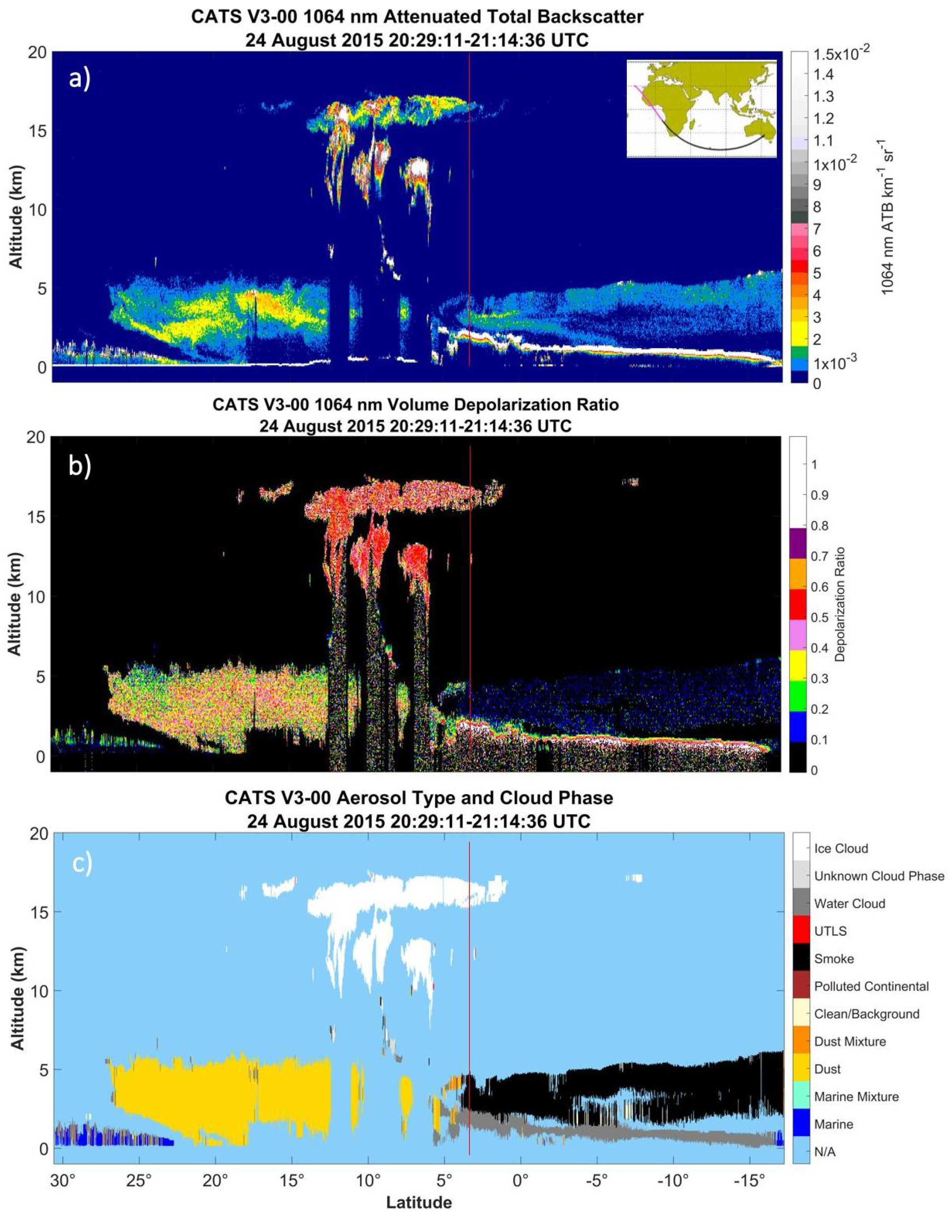
  • For absorbing aerosols, the absorption optical thickness increases with decreasing wavelength. This effect reduces the backscattered signal at 532 nm with respect to 1064 nm, such that the 532 nm backscatter is not sensitive to the entire vertical of the aerosol layer [40,41,42]. Because the 1064 nm wavelength is only minimally affected by aerosol absorption, the vertical extent of the absorbing aerosol layer is more fully captured from 1064 nm backscatter profiles rather than those from 532 nm [30].
Since CATS can detect the full vertical extent of the aerosol layer above the cloud, the CATS layer detection algorithm includes a routine to distinguish the cloud and aerosol layers as two separate layers when there is no separation between them.
The CATS Cloud-Embedded-in-Aerosol-Layers (CEAL) routine considers layers below 6 km, based on the assumption that the large majority of clouds embedded within aerosol layers will be confined to the lower part of the troposphere. Figure 1 and Figure 2 show an example of the CEAL routine identifying clouds embedded in aerosol layers. In Figure 2, the 1064 nm attenuated scattering ratio profile is greater than the threshold profile consistently from an altitude of 4.5 km down to 1.5 km. However, there is a distinct region between 1.5 km and roughly 2.5 km where the 1064 nm attenuated scattering ratio profile is nearly an order of magnitude greater than the region from 2.5 to 4.5 km. In this example, a single layer was identified before the CEAL routine correctly separated this layer into two distinct layers. Ultimately, the CATS L2O VFM algorithm identified these layers as smoke (2.5–4.5 km) lofted above a liquid water cloud (1.5–2.5 km), as shown in Figure 1c. This scenario is common in August over the Southeast Atlantic Ocean [30]. The logic used in the CEAL routine is discussed in further detail in Appendix A.
The CATS L2O layer detection is performed at two horizontal resolutions; 5 and 60 km. Only two resolutions were chosen in an attempt to simplify the layer detection algorithm. The 5 km resolution was chosen because it provided continuity with CALIOP and provided sufficient SNR and MDB to detect 95% of layers in nighttime simulations of the CATS system. The 60 km resolution improves daytime layer detection capabilities. In addition to using only two horizontal resolutions, the CATS layer detection algorithm processes the multi-resolution layer data differently as the different resolutions are run independently. No cloud-clearing or feature removal occurs after the 5 km run and before the 60 km run. The results are merged by mapping the layers detected at 60 km onto the 5 km grid (60 m vertical resolution). The boundaries of the two resolutions match exactly as there are twelve 5 km profiles per every one 60 km profile, so a single 60 km bin maps to twelve 5 km bins. Three tests, described in detail in Appendix A.2, are used to minimize artificial horizontal spreading of clouds in the 60 km data. The 60 km layer bins remaining after these tests are then merged with the 5 km layer bins. If a layer was detected at a given bin at either resolution, then a layer and the lowest resolution required to detect it are reported at that bin. Finally, geometric constraints (minimum layer thickness of 300 m, minimum inter-layer distance of 120 m, etc.) are enforced, eliminating and adding layer bins as necessary.
The primary purpose of using both 5 and 60 km horizontal resolutions for the CATS L2O layer detection is to increase the detection of aerosols and thin cirrus over land during daytime. Figure 3 shows the 1064 nm ATB for a daytime case on 12 September 2015 over deserts of the Middle East, averaged to 5 km (a) and 60 km (b). The layers detected (c) at 5 km (green) are primarily cloud layers with strong ATB, but red colors in Figure 3c show all the layers detected at 60 km that were missed at 5 km, including the aerosol plume between 22 N and 8 S latitude. The 60 km layer detection accounts for 50% of all ice clouds and 57% of all aerosols detected during daytime. Additionally, the 60 km layer detection at night enhances the detection of faint aerosol (9%) and ice cloud layers (5%).
A false positive rejection is applied during both 5 and 60 km layer detection before they are merged. The CATS false positive rejection scheme, like CALIOP’s, utilizes the feature-integrated backscatter (FIB, computed differently than iATB) of layers as a criterion for rejecting layers [36]. The FIB test checks whether the calculated FIB of a layer is less than a certain threshold (1.5 for Mode 7.2 night based on the expected MDB). The CATS scheme also considers the horizontal persistence of layers, which is described in detail in the CATS ATBD [37]. If a layer fails both the horizontal persistence test and the FIB test, the layer is omitted. A final, independent routine uses a t-statistic to determine whether the distribution of ATB values within a layer is significantly different than the distribution of ATB values in all “clear-air” bins within the profile. If the p-value is less than 0.1, the layer fails the test and is omitted.
The final major difference between the CATS L2O and CALIOP layer detections is that CATS includes a depolarization-based layer delineation algorithm (DeBLD). Under certain conditions, DeBLD divides a single layer into two separate layers based on the profile of 1064 nm volume depolarization ratio. DeBLD is performed when a layer is (1) below 18 km altitude, has a feature thickness greater than or equal to 840 m, and has not already been separated by the CEAL. Unlike CEAL, DeBLD can only split an input layer into two new layers. Operationally, CEAL and DeBLD are both utilized post-merge using 5 km backscatter and volume depolarization ratio. DeBLD only operates on nighttime data since the higher uncertainties of the daytime 1064 nm volume depolarization ratios reduce the accuracy of the routine, whereas CEAL operates on all CATS data (day and night).
Within a DeBLD candidate layer, wavelet analysis is performed on both the ATB and volume depolarization ratio values to identify boundaries to divide a layer into two sub-layers following the method of Davis et al. (2000) [43]. The determination on if and where the boundary is made is based on the sequence of steps described in Appendix A.3. To prevent the wrongful separation of two layers, DeBLD will not operate on layers in which greater than 35% of the bins have unreasonable volume depolarization ratio values (i.e., less than zero or greater than 1.0). Ultimately, DeBLD helps improve the accuracy of cloud-aerosol discrimination and aerosol typing for scenes where depolarizing aerosols (i.e., dust) are lofted but in contact with non-depolarizing aerosols (i.e., sea salt).

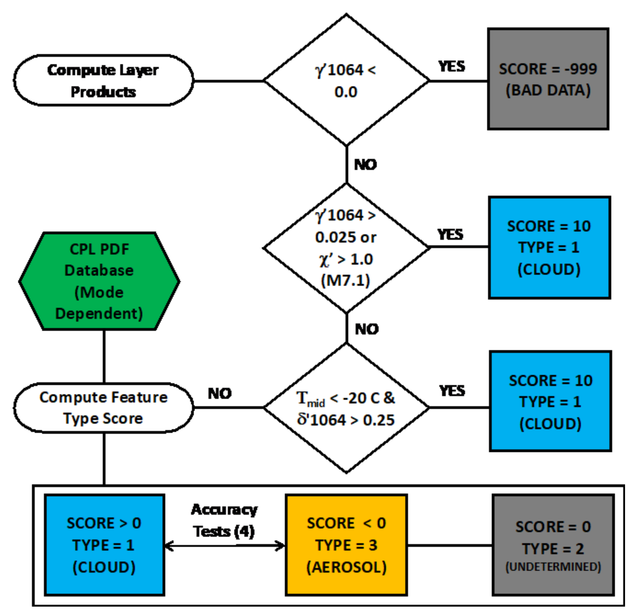
2.2. Cloud-Aerosol Discrimination

The CATS L2O CAD algorithm is a multidimensional probability density function (PDF) technique that is based on the CALIOP algorithm [44,45]. The PDFs were developed based on CPL measurements obtained from 11 field campaigns over 10 years (2003–2013) [46]. In total, over 1.6 million profiles with cloud layers present and nearly 1.8 million profiles with aerosol layers present were included in the dataset, which was limited to the top layer in any given profile. More information about the CPL data used for the CATS CAD is presented in the CATS ATBD [37]. Nearly all CPL layers with a layer-integrated attenuated backscatter at 1064 nm greater than 0.025 sr 1 are either liquid water clouds or ice clouds. Also, all features with a mid-layer altitude greater than 8.0 km and layer-integrated volume depolarization ratio at 1064 nm greater than 0.35 are ice clouds. Finally, features with a layer-integrated attenuated backscatter color ratio greater than 1.0 are typically clouds, with the exception of some elevated aerosols that are likely large dust particles.
The CATS L2O CAD algorithm is driven by a probability function where PDFC and PDFA are the multidimensional PDFs, respectively, for clouds and aerosols. For CATS, there are three PDFs used with attributes (i). Data quality, computing time and ancillary data rates must be considered when selecting attribute dimensions for operational PDFs. For the data used in this paper, the dimensions are the layer-integrated attenuated backscatter ( γ ) at 532 nm, the layer thickness ( Δ Z), layer-integrated 1064 nm volume depolarization ratio ( δ ), and the midlayer altitude (Z t o p ). The probability score (−100 to 100) for these PDFs are computed using Equation (1):
P P D F i = P D F C i P D F A i P D F C i + P D F A i × 100 .
The main objective of the CATS L2O CAD algorithm is to compute the Feature Type Score, which is an integer value ranging from −10 to 10 for each atmospheric layer. The sign of the Feature Type Score identifies a layer as either cloud (positive) or aerosol (negative), while the magnitude of the Feature Type Score represents the confidence in our classification (Table 1). A value of 10 indicates complete confidence that the layer is a cloud, while −10 indicates confident classification of an aerosol layer. When the Feature Type Score equals 0, the layer is just as likely to be a cloud as it is an aerosol and thus the classification is undetermined. If the optical and physical properties of the layer are considered invalid for clouds and aerosols, these layers are assigned a Feature Type Score of −999.
The flow of the CATS operational CAD algorithm is shown in Figure 4. First, the CAD algorithm computes the layer products, which include γ at both 532 and 1064 nm, χ , δ at 1064 nm, Z m i d , and T m i d . Before classifying an atmospheric layer, the L2O CAD algorithm declares the layer invalid if the layer integrated γ 1064 is less than 0. Then, the algorithm identifies high confidence cloud layers (Feature Type Score = 10) as those layers with a γ 1064 greater than 0.03 sr 1 . No aerosols layers identified in the CPL data were found above these threshold values. In the first year of CATS data, few aerosol layers were observed below temperatures of −20 C, with the exception of volcanic plumes, which had 1064 nm volume depolarization ratios less than 0.15 (typical of plumes that consist mostly of SO 2 ). If the T m i d is less than −20 C and the δ 1064 is greater than 0.25, the layer is classified as a high confidence cloud and the Feature Type Score is set to 10.
If a layer does not meet any of these criteria, then the PDF technique is used to determine whether the layer is composed of aerosol or cloud. The PDFs are employed to compute the Feature Type Score that is reported within the CATS L2 products using Equation (2), where T P D F i is the total number of data points for the specific attribute i.
C A D = ( P P D F 1 100 ) T P D F 1 + ( P P D F 2 100 ) T P D F 2 + ( P P D F 3 100 ) T P D F 3 T P D F 1 + T P D F 2 + T P D F 3 × 10 .
The PDF CAD technique does have limitations. The single wavelength (1064 nm) nature of the CATS Mode 7.2 data makes accurate cloud-aerosol discrimination a challenge in complex mixtures of clouds and aerosols near the surface using the PDF technique. Furthermore, multiple scatter effects from CATS often resulted in depolarizing liquid water clouds that are not represented in the CPL measurements used for the PDFs since CPL experiences small (<5%) multiple scattering effects [46]. Finally, aerosol plumes in the UTLS were rarely observed in the CPL data used for the PDFs, but CATS observed several volcanic plumes and smoke plumes from pyrocumulonimbus during its operations. These plumes typically have weak backscatter and depolarization signals [47]. Thus, any layer with a base altitude greater than the MERRA-2 tropopause height with a γ 1064 less than 0.03 sr 1 and δ 1064 less than 0.25 is assigned a Feature Type Score of −10 since overshooting cloud tops typically have layer-integrated attenuated backscatter values greater than this threshold. While Polar Stratospheric Clouds (PSCs) do meet these thresholds, the ISS orbit does not travel to higher latitudes where PSCs are prevalent.
To overcome these limitations and improve the CATS L2O CAD algorithm performance for these circumstances, the algorithm was updated for V3. Additional tests based on horizontal persistence, relative humidity, cloud fraction and integrated perpendicular backscatter tests are utilized in the CAD algorithm. The Feature Type Scores are then updated for layers that pass or fail these tests. If a layer passes multiple tests, the score becomes more confident (±9 or 10) if it is not already the highest confidence. If the layer only passes one test, the Feature Type Scores only increases/decreases by 1 resulting in more layers with a Feature Type Score of ±6 or 7 than in previous versions. Details for each of the additional CAD accuracy tests are in Appendix A.4.

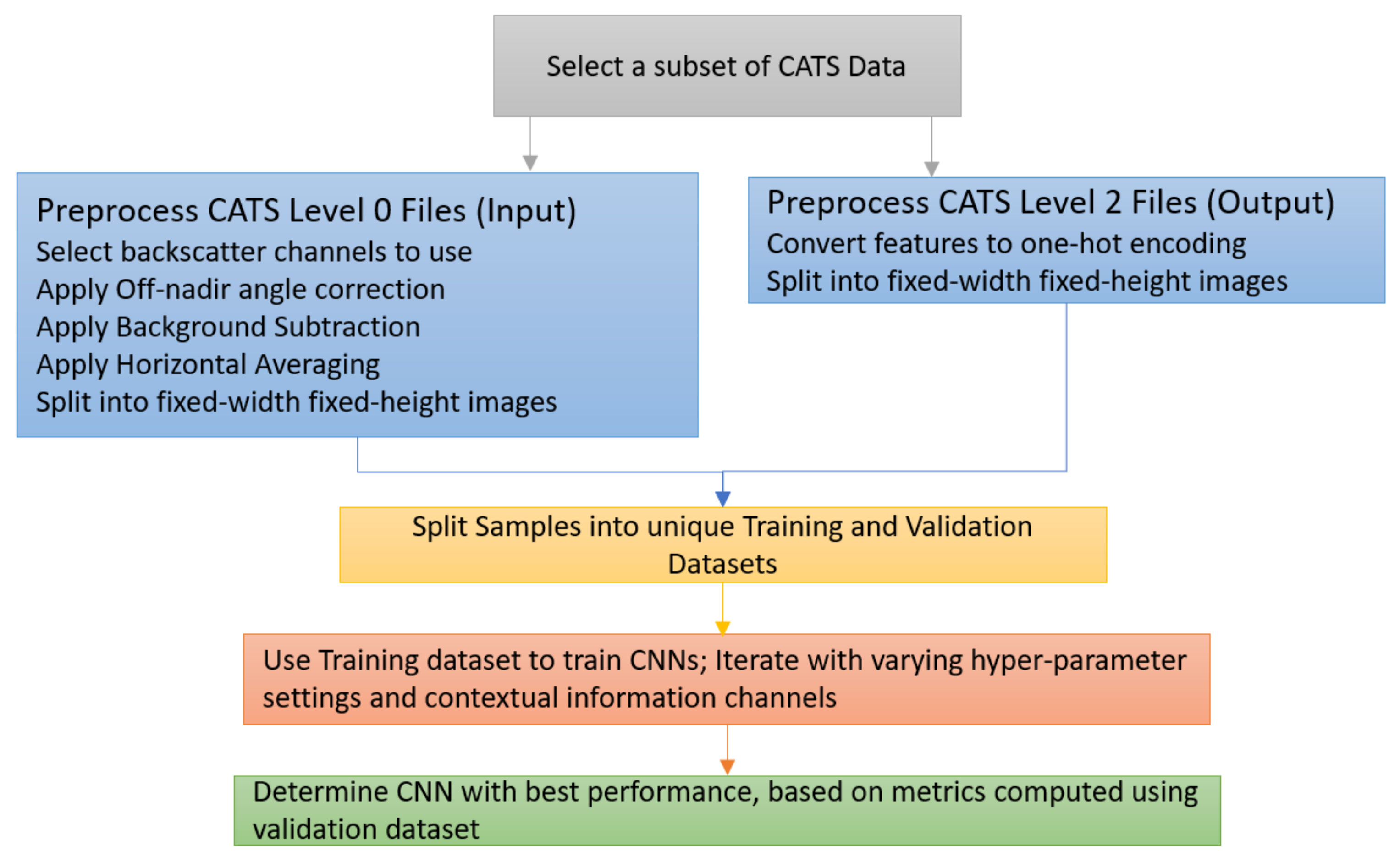
3. Machine Learning Algorithms

Recent studies have performed statistical comparisons of CATS L2O cloud and aerosol properties with CPL, CALIOP, the European Aerosol Research Lidar Network (EARLINET) and Atmospheric Radiation Measurement (ARM) lidar measurements. CATS nighttime layer detection capabilities are robust, with the ability to detect aerosol features with aerosol optical depths as low as 0.08 [33]. However, Dolinar et al. (2020) [48] shows that, during daytime, CATS underestimates thin cirrus cloud occurrence compared to CPL due to poor SNR prohibiting detection even at a coarse horizontal resolution of 60 km.
Photon counting detectors, such as the ones employed by the CATS instrument, are characterized by a Poisson noise distribution that is proportional the square root of the signal. During the day, the solar background signal can be much larger than the signal returns from clouds and aerosols, making these features difficult to detect. Averaging the data to a coarser horizontal resolution has been the standard way to increase SNR and thus allow features (cloud and aerosols) to be more easily detectable. However, there exist algorithms to remove noise from data in the form of images or arrays, which retain the original resolution, and these types of algorithms can be applied to lidar data (e.g., Figure 1a,b). Given the scientific community’s desire for finer resolution data products, four candidate denoising algorithms are considered in this study—Principal Component Analysis (PCA) [49], Wavelet Denoising [50], Butterworth Filtering [51], and Gaussian Filtering [52]. The four denoising techniques are described in detail in Appendix B.1.
The lower daytime SNR of the CATS data can also impact the operational algorithm’s ability to discriminate aerosols from clouds. Noel et al. (2018) [26] shows that CATS detected less Planetary Boundary Layer (PBL) and midlevel clouds compared to several EARLINET and ARM sites, likely attributed to (1) misclassification of clouds as aerosols in the CATS operational CAD algorithm and (2) high-altitude clouds impairing CATS ability to detect these lower clouds. Dolinar et al. (2020) [48] also showed that CATS algorithms can misclassify the cloud edges of daytime thin cirrus as aerosols. Lee et al. (2019) [27] compared CATS and CALIOP aerosol extinction profiles and found good agreement, within 5%, for aerosols over land. However, over water and during daytime, CATS extinction coefficients below 1 km altitude are 10–25% higher than CALIOP. They hypothesize that one possible explanation for these differences is that the CATS feature detection algorithm does not extend near-surface aerosol layer base heights down to the surface.
Several ML techniques exist that can be applied to CATS data for improved cloud-aerosol discrimination. Autoencoding is a neural network technique that is a widely-studied method in ML to accomplish data compression. Autoencoders work by training a neural network to reproduce N-dimensional input, using one or more k-dimensional hidden layers. The first layers of the neural network can be interpreted as dimensional reduction from N-dimensional input to a k-dimensional encoding. The remaining layers of the neural network represent a decoding of the k-dimensional data back to N-dimensional space. When trained correctly, this forces the neural network to learn how to interpret the signal in the input, without possessing enough neurons in the hidden layers to enable memorization of the noise in the training data. CNNs are one of the most successful ML techniques for image processing, especially given that the capability of graphics processing units (GPUs) has grown exponentially. To the authors’ knowledge, this is the first publication to apply a CNN to space-based cloud-aerosol lidar data.

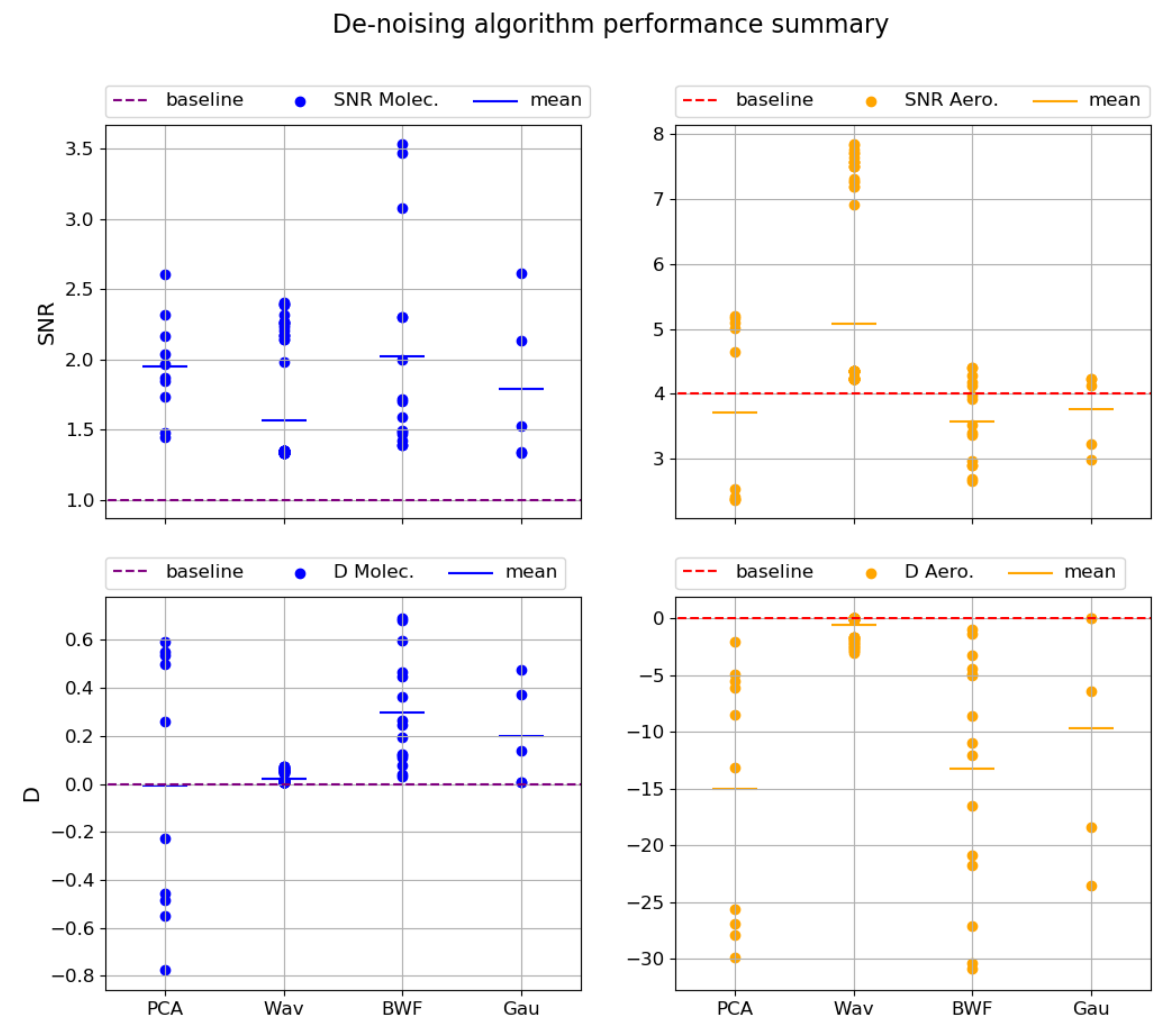
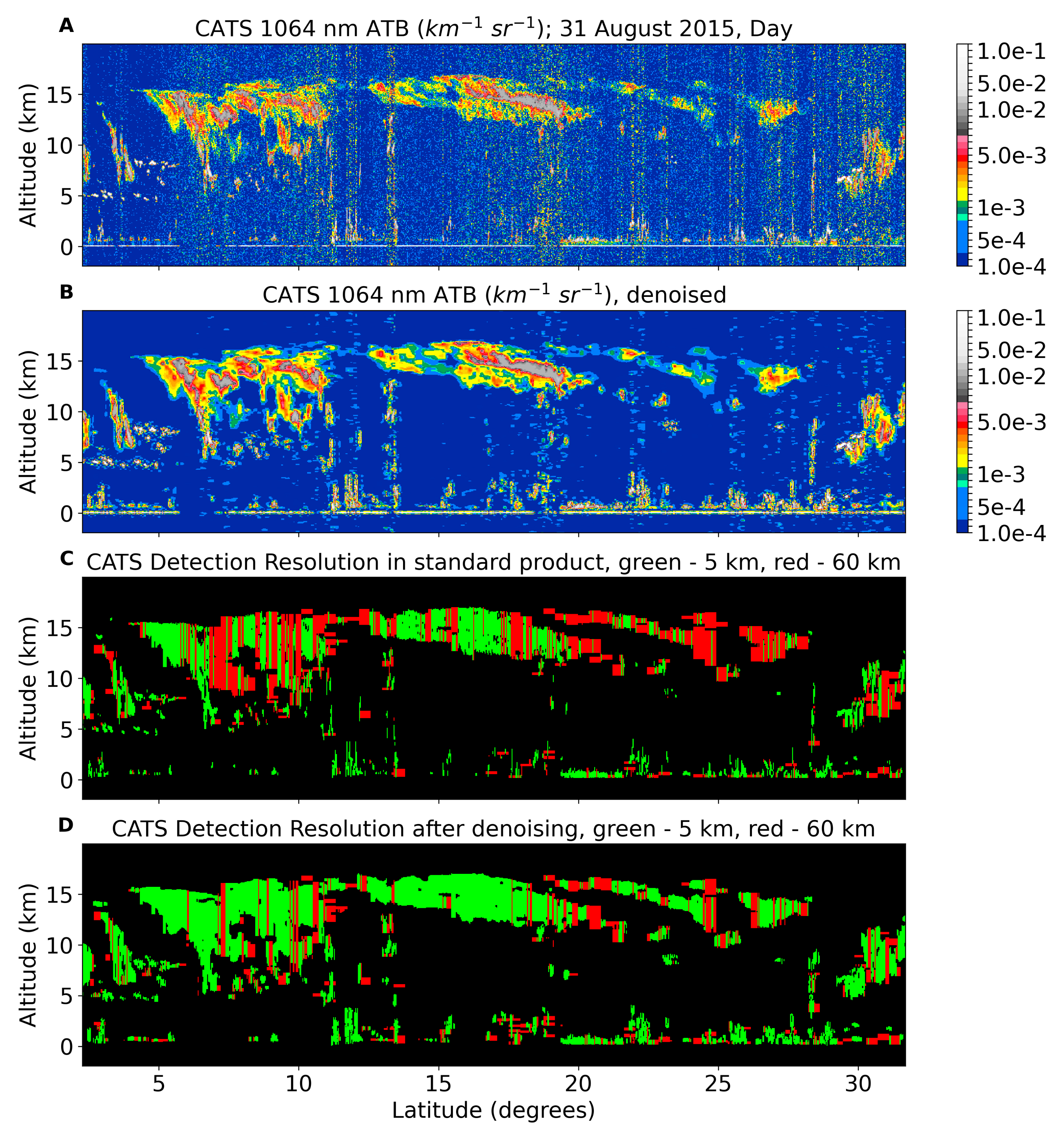
3.1. Denoising Technique

Each of the four algorithms (Principal Component Analysis, Wavelet, Butterworth, Gaussian) were tested on simulated daytime 532 nm space-borne photon-counting lidar data to assess their performance. Two metrics were computed to do so—SNR (Equation (3)), and the deviation from the expected signal, D (Equation (4)). In Equations (3) and (4), E is the expected signal, N is the noise, and A is the observed signal. All signals are in terms of photon counts. E is the signal that would be expected from a perfect detector with no noise. A is the simulation of how a real detector would measure the “true” signal E. These metrics were computed separately for the molecular and aerosol (particulate) components of the signal.
S N R = | E + N | R M S ( N )
D = m e a n ( A E ) .
For each of the algorithms, a variety of different reasonable parameter settings were tested. Table 2 lists the different tunable parameters for each of the algorithms.
Figure 5 summarizes the results of the test on the simulated data. The left column plots show the metrics computed on the molecular signal (blue), and the right column plots are for aerosol signal (orange) for each of the four algorithms. Higher SNR generally means better performance. However, the deviation, D, should optimally be close to zero. If the deviation is too great after the technique is applied, either a bias or distortion is being introduced by the denoising algorithm which indicates that the algorithm is incompatible with traditional elastic backscatter lidar data processing algorithms since they heavily leverage comparison to theoretical (expected) Rayleigh signal.
Based on the results in Figure 5, the Wavelet algorithm provides the right balance of an increased SNR and minimal D to allow for incorporation into traditional lidar data processing. The details of the precise input parameters for the wavelet algorithm selected for further testing is in Appendix B.2. Following selection of the wavelet algorithm parameters, tests were conducted to show that denoising the ATB, as opposed to the raw photon counts, did not shift the clear-air signal away from theoretical Rayleigh. For a comparison of performance improvements, the Wavelet denoising algorithm was applied directly to CATS attenuated total backscatter (ATB) and then the current Level 2 CATS processing algorithms were applied. Performance improvements from the additional denoising step of the ATB are discussed in detail in Section 4.

3.2. CNN Technique

A CNN is a supervised machine learning algorithm that has been used for image feature recognition. Commercial applications of CNNs include a wide range of object detection and semantic segmentation problems [53]. Additionally, CNNs have been utilized to accurately estimate tropical cyclone intensity using satellite imageries [54] and hailstorm detection in radar imagery with accuracy superior to existing techniques [55]. After the layer architecture of the CNN is instantiated, the model is trained from truth datasets, developing the knowledge to correctly predict features in the image. While the training of a CNN can take a substantial amount of time, the predictions are extremely fast when compared to traditional algorithms or a manual approach. To improve the speed in which lidar data can be disseminated to the public and determine the feasibility to provide real-time layer-typing products, a set of CNNs have been developed to predict the locations of clouds and aerosols in CATS lidar data.
To train and validate the CNNs, a one-to-one mapping was determined between the CATS Level-0 (L0) files from the instrument and the processed CATS Level-2 (L2) product files to serve as input and output examples to the model, respectively (Figure 6). For each CNN, one month of CATS data (October 2017) was used to form a set of independent sample inputs and corresponding outputs. One month of data was chosen because it was large enough to contain a representative sampling of cloud and aerosol scenes, yet small enough to train the CNN relatively quickly. Those samples were then split into two distinct groups, a validation, and a training dataset where the validation dataset comprised of 20–25% of the total number of samples [56]. No optimization has been done for the split percentage between validation and training datasets thus far. For both the validation and training dataset input samples, some traditional pre-processing corrections were made to ensure a correct mapping and improve CNN performance from the raw L0 backscatter profiles. These consisted of subtracting the solar background, averaging the vertical profiles to match the horizontal resolution of the L2 products, correcting for small off-nadir angles and then placing the records in a fixed vertical frame. In addition, the data also requires a fixed horizontal dimension to be input for the CNN so the samples are split into images for every 256 CATS L2 records.
The U-Net architecture utilized by Ronneberger et al. (2015) [57] was selected as the CATS CNN architecture. Further detail on how the U-Net architecture was implemented has been included in the Appendix B.3. Once the CNN models were instantiated, they were then trained using various combinations of hyper-parameter settings that effect the training efficiency and prediction accuracy. In addition to varying the hyper-parameters, the number of input channels were also varied. For the CNNs different combinations of the following inputs were used: 1064 nm perpendicular signal, 1064 nm parallel signal, 1064 nm total signal, latitude, longitude, and surface type. The latter three ancillary data inputs had to be expanded from 1D into 2D arrays corresponding to the lidar signal for compatibility with the CNNs. To achieve this, the ancillary data value for a given profile was repeated for every vertical bin.
The F1-score and weighted-f1 metric have been used to compare the accuracy of the models using the independent validation dataset. Precision and recall metrics are used to compute the F1-score as listed in Equations (5) thru (7). Calculating precision and recall requires first finding the number of (1) True Positives, the population of pixels a feature is correctly predicted, (2) False Positives, the population of pixels a feature is predicted and none exists at that location, and (3) False Negatives, the population of pixels where the feature is not predicted at a location that does indeed have that feature. The weighted F1-score is calculated by multiplying a factor to the individual feature F1-score proportional to the feature population in the truth dataset. The model used for comparison to the CATS traditional operational algorithms was chosen based on the weighted F1-score metric. As with other applications utilizing fully convolutional neural networks (FCN), [53,54] we determined that the Jaccard-distance loss method produces better outcomes with respect to the commonly-used cross entropy loss function. The CATS data have features that are sparsely distributed, which justifies this result. Applying batch normalization, as was used by Ronneberger et al. (2015) [57], was also found to be optimal for model performance. The CNN models chosen for both day and night used 1064 nm perpendicular, parallel and total channels. The ancillary latitude, longitude, and surface type did not provide a performance advantage.
p r e c i s i o n = T r u e P o s i t i v e s T r u e P o s i t i v e s + F a l s e P o s i t i v e s
r e c a l l = T r u e P o s i t i v e s T r u e P o s i t i v e s + F a l s e N e g a t i v e s
F 1 s c o r e = 2 × p r e c i s i o n × r e c a l l p r e c i s i o n + r e c a l l .

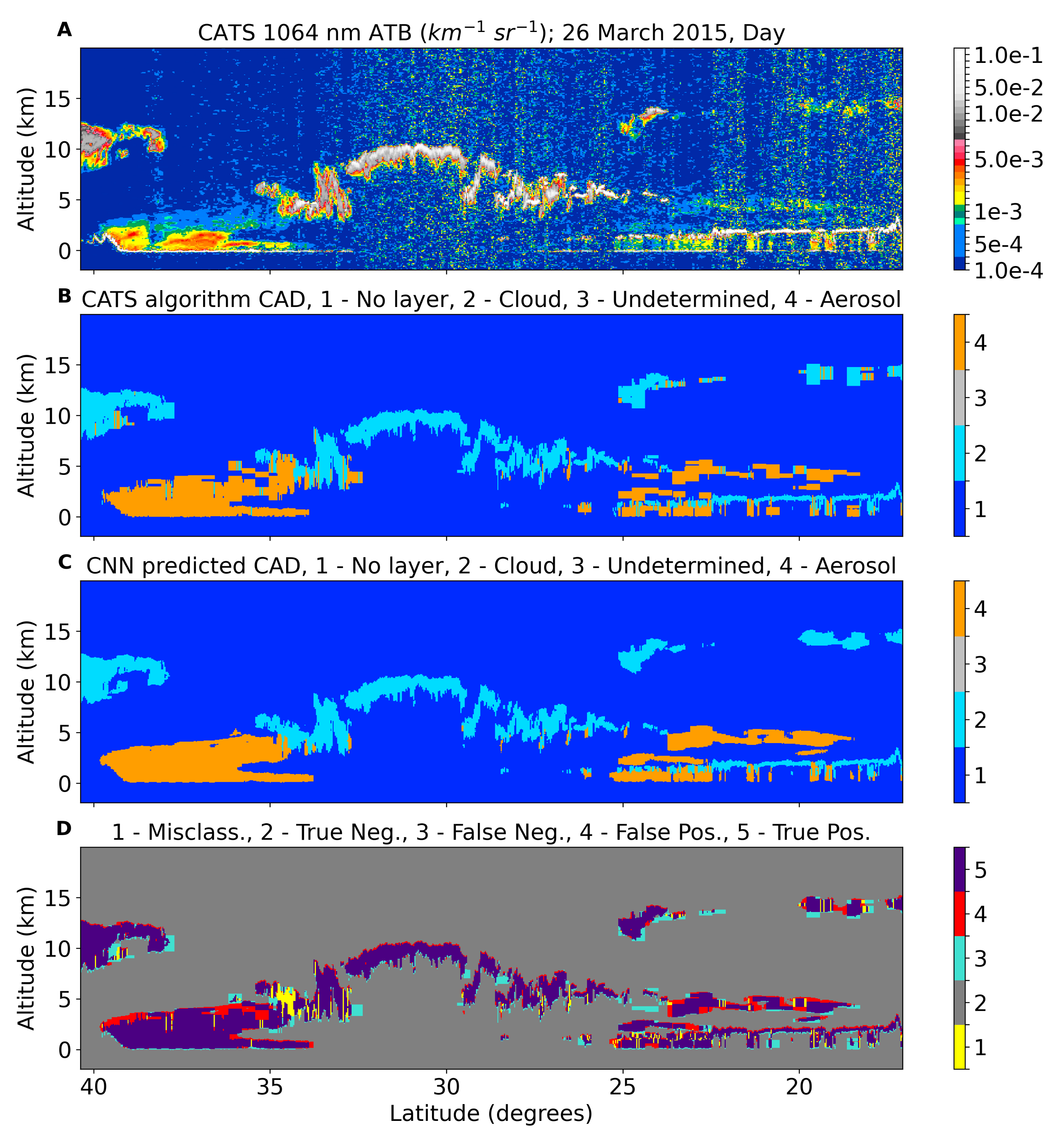
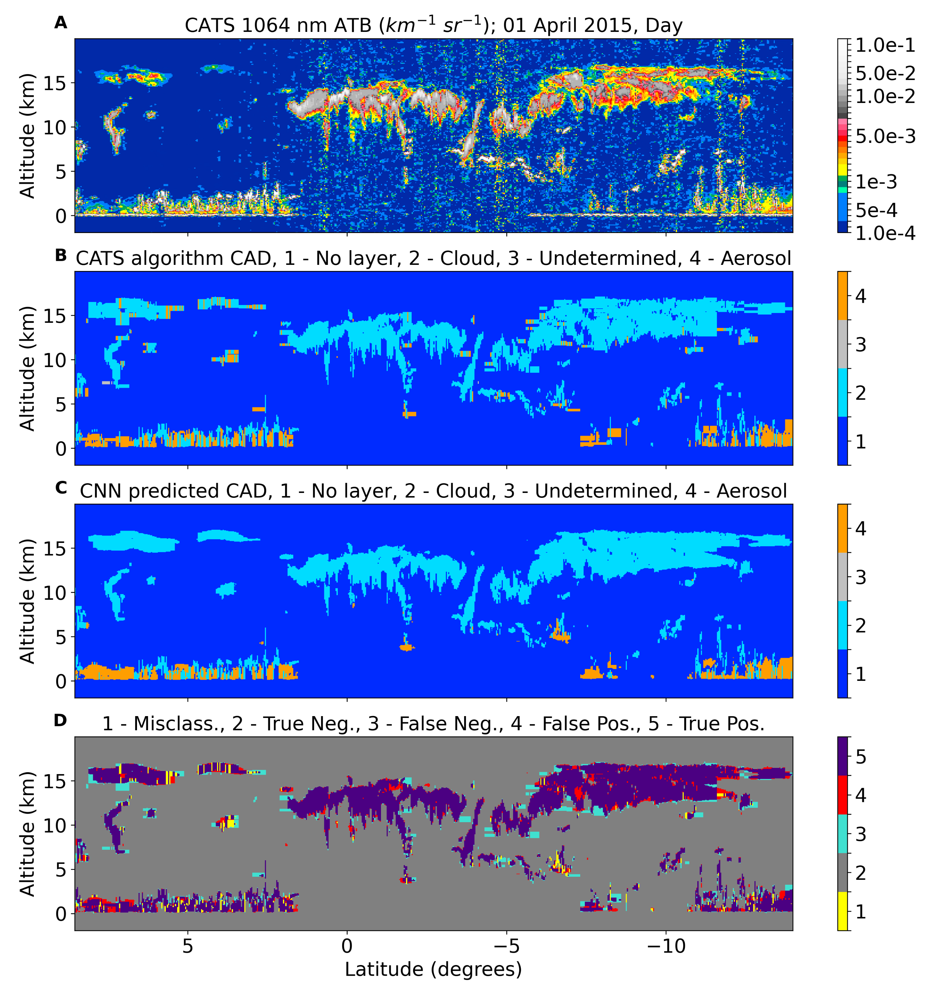
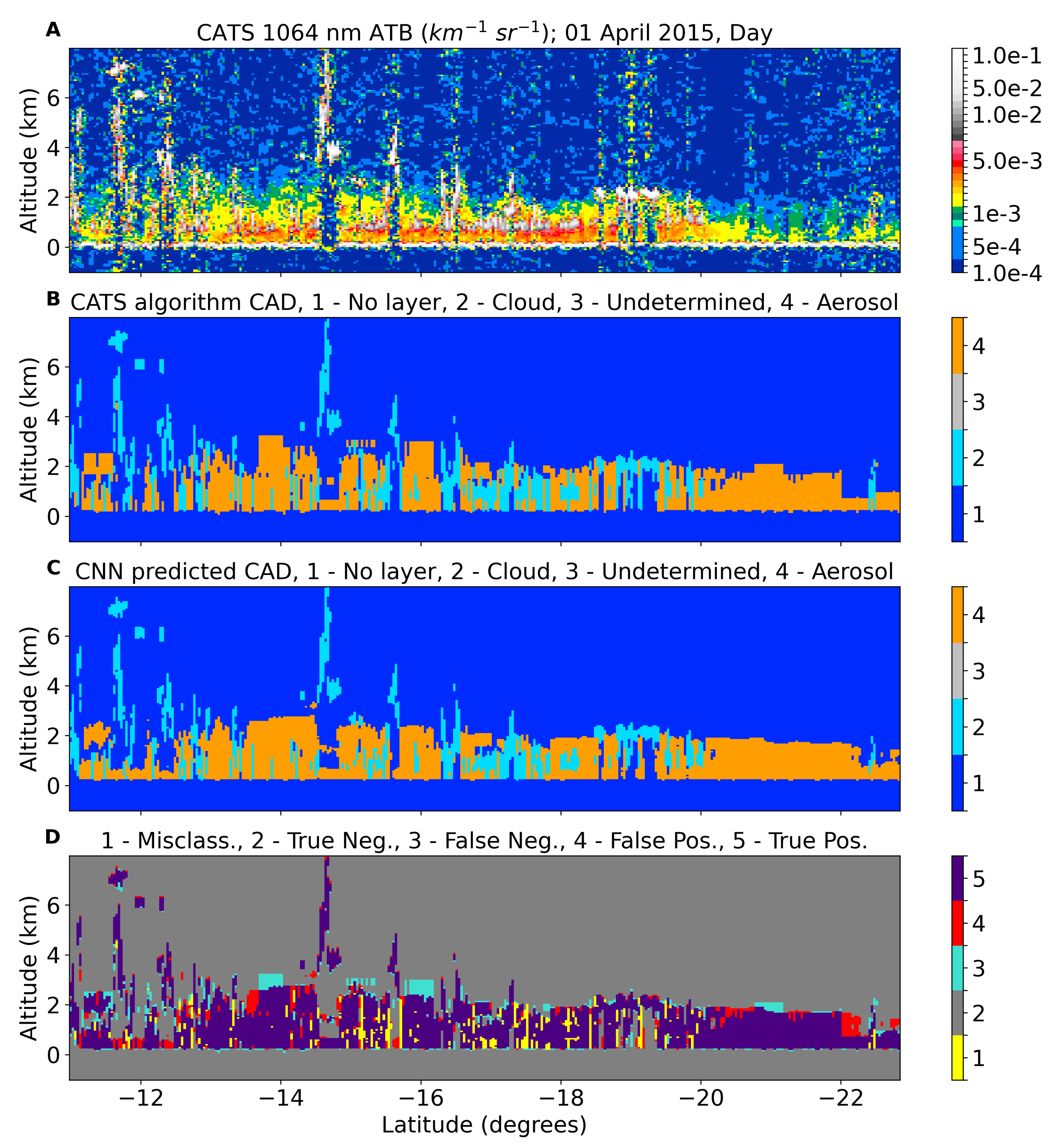
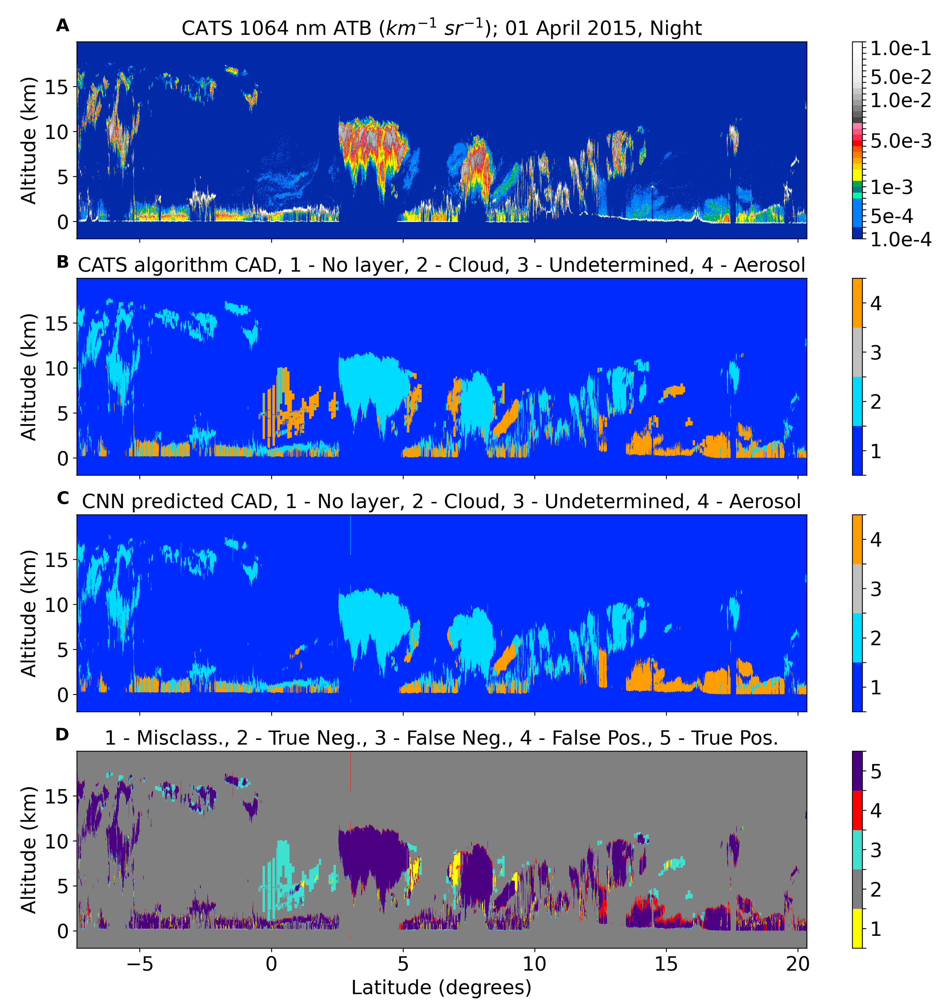
4. Comparison of ML Techniques with Operational CATS Data Products

The goal of the Wavelet denoising technique is to improve the daytime CATS SNR, thus enabling the operational layer detection technique to detect layers at finer horizontal resolutions. While 95% of all cloud layers and 91% of all aerosol layers are detected at 5 km in nighttime CATS data, only 50% of ice clouds and 43% of aerosols are detected at 5 km in daytime CATS data. The denoised CATS Level 1B data described in Section 3.1 was run through the operational L2 data processing algorithms, including the 2-resolution layer detection algorithm. An example of a CATS daytime scene on 31 August 2015 is shown in Figure 7. Multiple cirrus clouds with variable optical depths are visible to the eye in the operational 1064 nm attenuated backscatter (A). While 47.9% of these layers were detected at a horizontal resolution of 5 km (C, green), 52.1% required the coarser 60 km horizontal resolution (C, red). The Wavelet denoised 1064 nm attenuated backscatter (B) shows significantly less noise, resulting in 62.5% more clouds detected at the finer 5 km horizontal resolution. While this denoising technique enables the operational layer detection technique to detect layers at finer horizontal resolutions, 33.4% of layers still required 60 km averaging given CATS low SNR during daytime.
The CNN technique was performed at the standard 5 km horizontal resolution of the CATS standard data products, so it provides another pathway to detecting layers at finer horizontal resolutions. Figure 8 shows the 1064 nm attenuated backscatter (A), the operational CATS CAD results (B), the CNN predicted CAD results (C), and a visual comparison between the operational and CNN techniques (D) for a daytime case on 26 March 2015 with ice clouds, aerosols, and liquid water clouds present. The visual bin-by-bin comparison plots (panel D) have a key with labels that can be interpreted as follows:
  • Misclass—when the CNN and CATS L2 agree there is a feature (either cloud, aerosol, or undetermined), but do not agree on the type
  • True Neg—when both the CNN and CATS L2 agree there is clear air (no feature)
  • False Neg—when the CNN classifies a bin as clear air and CATS L2 identifies that bin as any feature type
  • False Pos—when the CNN classifies a bin as any feature type (either cloud, aerosol, or undetermined) and the CATS L2 identifies it as clear air
  • True Pos—when the CNN detects a feature and its classification matches the CATS L2
Bins that are assigned as clouds or aerosols in the operational CATS CAD due to the 60 km horizontal averaging appear “blocky” in Figure 8B, as demonstrated in the ice clouds above 8 km (light blue) and the “False Negative” denotation (light blue) in Figure 8D. Furthermore, bins with weak attenuated backscatter within aerosol layers are captured by the CNN technique that are not detected in the operational CAD algorithm, as demonstrated by the “False Positive” assignment (red) in Figure 8D. This results in more homogeneous aerosol layers (Figure 8C, orange) that appear consistent with the attenuated backscatter data, despite the CNN technique only utilizing a 5 km horizontal resolution.
With regards to cirrus clouds, two issues with the CATS operational CAD algorithm during daytime identified in Section 2 and Section 3 are (1) cloud edges falsely identified as aerosol and (2) layers not detected even at 60 km horizontal resolutions. The CNN technique improves upon both these issues. Figure 9B shows bins near the cloud edges (light blue) that were identified as aerosol (orange) in the operational CATS CAD algorithm. The CNN technique identifies these bins as clouds (Figure 9C). The CNN technique also detects more tenuous parts of these clouds that were not detected by the operational CATS CAD, as shown as “False Positive” in Figure 9D (red). Furthermore, the CNN was able to replicate much of the operational CATS CAD cloud detections (Figure 9D, purple) and do so at the finer 5 km resolution. These 3 improvements provide a much more robust cirrus dataset during daytime operations.
Misclassification of clouds and aerosols in the CATS operational CAD algorithm near the surface was a possible explanation for differences in cloud and aerosol properties observed between CATS and other lidar sensors [26,27]. Figure 10 is a classic example of a complex scene of mixed clouds and aerosols within the PBL observed by CATS on 1 April 2015 over New Caledonia. The CNN technique (Figure 10C) classifies some bins as aerosols that appear to be misclassified by the CATS operational CAD algorithm as clear-air given the 1064 nm ATB (Figure 10A) yields magnitudes consistent with aerosols in these bins (Figure 10D, red). While it is difficult to differentiate the type of feature using the CATS 1064 nm ATB alone, the CNN technique identifies more aerosols below the cumulus clouds, as demonstrated in Figure 10D (yellow). While these results are shown for a horizontal resolution of 5 km, they suggest that the CNN technique could be a powerful tool for cloud detection and clearing at the CATS native resolution (350 m), which would reduce potential cloud contamination of aerosol properties for features reported as aerosols.
While the CNN technique presented here demonstrates improvements in layer detection at finer resolution and cloud-aerosol discrimination during daytime, this new ML technique also has limitations. At nighttime, the CNN technique only exhibits minor improvements to layer detection and CAD and, in some cases, actually performs worse than the operational CATS CAD algorithm. Figure 11 shows a nighttime case on 1 April 2015 with weakly scattering aerosol plumes lofted into the free troposphere in the same altitude regions as cirrus clouds. The aerosol plume between 1 S and 3 N latitudes is so optically thin (AOD of 0.02) that the CNN technique does not detect the feature at the 5 km horizontal resolution, whereas the operational CATS layer detection algorithm is sensitive to this layer at the 60 km horizontal resolution (Figure 11D, teal). The CNN technique does detect features with weak backscatter intensities (like lofted aerosols) around 7 N latitude adjacent to cirrus clouds with strong backscatter intensities (Figure 11C), but it classifies these optically thin features as clouds when the operational CATS CAD algorithm classifies them as aerosols (Figure 11D, yellow). Since the CNN model is based on the statistical significance of the features in the training dataset, and free tropospheric aerosol layers are far less frequent in the CATS training dataset compared to cirrus clouds, the CNN misclassifies these layers as clouds. Thus, training datasets must be carefully selected to optimize performance of the CNN technique. Further experiments are needed to assess the amount of samples needed for specific atmospheric features to overcome these inaccuracies.

5. Discussion

To quantify the differences between the CNN technique and operational CATS CAD algorithm, the CNN technique was run on the entire month of CATS data for September 2015. Confusion matrices for the nighttime and daytime data are shown in Figure 12a,b, respectively. At both nighttime and daytime there is good agreement for clear-air bins (>97%). However, this is to be expected since the majority of lidar bins are “clear-air”. Due to the ambiguity and low population of the undetermined classification in the training dataset, the CNN model never predicts layers as undetermined, so those layers classified as such in the operational CATS CAD algorithm were primarily identified as clouds (55–65%) by the CNN technique, while a smaller percentage were classified as clear-air (24–39%) or aerosol (5–11%). For bins detected as clouds by the operational CATS CAD algorithm, the agreement is better at night (91.3%) than during the daytime (78.3%). A small percentage (2–3%) of cloud bins from the operational algorithms were identified as aerosols by the CNN technique, most likely found in complex PBL scenes as shown in Figure 10. The agreement for the two techniques was worst for aerosols, especially during daytime (68.1%). Roughly 9% of these layers, both day and night, were classified by the CNN technique as clouds. Most of these cases were likely the cirrus cloud edges misclassified by the operational CATS CAD algorithm as aerosol, such as the example in Figure 9. The largest discrepancies between the two techniques are found when the CNN technique predicted clear-air bins, but the operational CATS CAD algorithm identified a cloud or aerosol. At nighttime this occurred 5.6% and 7.2% of the time for cloud and aerosol features, respectively. Given the high SNR nighttime CATS 1064 nm data and strong performance of the CATS layer detection algorithm at night, these cases are likely optically thin features that the CNN technique failed to detect at a 5 km horizontal resolution, as shown in Figure 11. During daytime, there are more instances when the operational CATS CAD algorithm detects features at 60 km horizontal resolutions, which falsely increases the size of these layers when mapped back to 5 km resolution. As demonstrated in Figure 8, the CNN technique, which only detects at 5 km, appears to better capture the true shapes of these features as indicated by the higher frequencies of clear-air bins (19.4% for clouds and 22.7% for aerosols) observed in the daytime statistics for bins when features were present in the standard CATS data products.

6. Conclusions

The Cloud-Aerosol Lidar with Orthogonal Polarization (CALIOP), aboard the CALIPSO satellite, has provided vertical profiles of clouds and aerosols critical to the science community since 2006. The CATS lidar augmented the CALIOP lidar data record by providing similar data from the ISS for 33 months with diurnal information. While these systems have limitations, such as degraded daytime signals by noise from solar background light and limited information content for feature typing, ML techniques like the CNN demonstrated in this paper can overcome some issues such as coarse daytime detection resolutions and PBL cloud-aerosol discrimination but not without limitations for detecting subvisible features during nighttime. The wavelet denoising and CNN techniques presented in this paper increased the CATS 1064 nm SNR by 75%, increased the number of layers detected (any resolution) by 30%, and enabled detection of 40% more atmospheric features during daytime operations at a horizontal resolution of 5 km compared to the 60 km used for daytime CATS operational data products. This equates to a factor of 12 improvement in horizontal resolution of daytime CATS feature typing data products for over 40% of atmospheric features.
Further CNN model training should be explored since the training dataset is critical to the performance of the CNN technique. While training datasets do not need to be comprised of more than 20–25% of the total number of samples, they do need to be representative of the data the model will attempt to predict. For space-based backscatter lidar data, this means training datasets should include some number of examples of less-prevalent atmospheric features such as subvisual cloud and aerosol layers (OD < 0.03), as well as volcanic or smoke aerosol layers in the upper troposphere-lower stratosphere altitude region. Once such a technique is optimized, future processing of these lidar datasets should employ a combination of traditional techniques and ML methods to improve the accuracy, resolution, and utility of the standard data products, especially during daytime. Such improvements enable researchers to more confidently combine passive daytime measurements with lidar observations for accurate data analysis.
ML algorithms can also be incorporated into future space-based lidar missions and performed on raw data to enable near-real time (NRT) atmospheric feature height and type data products that have short latencies (<1 h processing time). Such NRT data products can be used as aerosol model input to improve monitoring and forecasting of volcanic and smoke plumes. Currently these applications stakeholders do not use lidar data products operationally because shorter latencies and more accurate data products are required. While the results shown in this paper are for a horizontal resolution of 5 km, they suggest that the CNN technique could be a powerful tool for cloud detection and clearing, and even aerosol detection at finer horizontal resolutions (<500 m) that are of interest to the air quality community. Machine learning tools, such as the ones presented in this paper, can be infused into future lidar instrument concepts and missions to reduce the noise in daytime lidar signals and facilitate the development of smaller, more affordable lidar systems.

Author Contributions

J.E.Y. aided in experimental design, drafted the manuscript, and responded to reviewers. P.A.S. and A.K. designed the experiments, performed the analysis, and created visualizations. E.P.N. and K.E.C. aided in experimental analysis and manuscript drafting. D.R. and N.D. aided in the creation of the visualizations. M.J.M. obtained funding and provided guidance for the analysis. All authors have read and agreed to the published version of the manuscript.

Funding

The funding sources for this paper are: (1) the ISS NASA Research Office (NRO) for funding the CATS instrument, (2) the NASA Science Mission Directorate (SMD) for funding the operational CATS data products and processing algorithms, and (3) the NASA Earth Science Technology Office (ESTO) for funding the development of the machine learning algorithms presented in this paper.

Institutional Review Board Statement

Not applicable.

Informed Consent Statement

Not applicable.

Data Availability Statement

All CATS data products used in this paper and documents such as the data products catalog, release notes, and algorithm theoretical basis documents (ATBDs) are available at the CATS website (https://cats.gsfc.nasa.gov) and/or the NASA Atmospheric Science Data Center (https://asdc.larc.nasa.gov/).

Acknowledgments

The authors would like to thank Mark Vaughan (NASA Langley Research Center) and Sharon Rodier (SSAI) for their help and guidance in the development of the operational CATS processing algorithms.

Conflicts of Interest

The authors declare no conflict of interest.

Appendix A. Details of CATS Vertical Feature Mask Algorithms

Appendix A.1. Description of Cloud-Embedded-in-Aerosol-Layers (CEAL) Method

For each layer under consideration a threshold ATB value is calculated by multiplying the median ATB of the layer by a threshold factor of 9. The threshold ATB value is compared to the maximum ATB of the layer. If the maximum is greater than the threshold, then a cloud boundary search is conducted as follows:
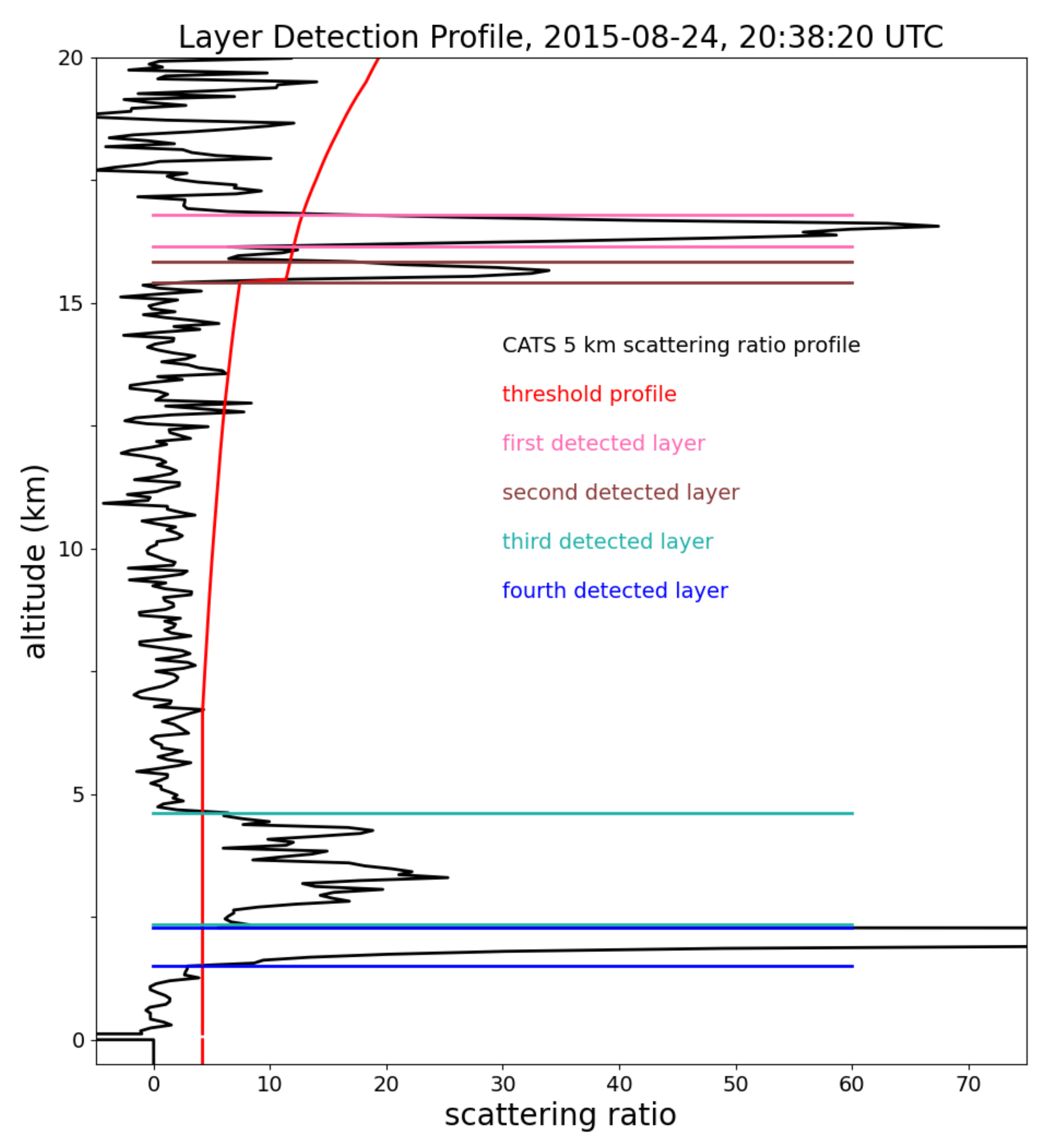
  • From the altitude bin of the maximum ATB, a search begins upward (in altitude) bin by bin until the ATB value is below the threshold.
  • This bin is assigned as the top of the cloud layer.
  • The base of the cloud layer is found analogously by searching downward from the maximum until the same conditions are met.
CEAL can identify up to 2 clouds within a single combined cloud-aerosol layer. Regions of the original candidate layer outside of the identified clouds are considered separate layers as long as they have a vertical thickness of at least 300 m.

Appendix A.2. Logic for Preventing the Artificial Spreading of Clouds

To minimize artificial horizontal spreading of clouds, the following tests are applied to the 60 km CATS data:
  • If >75% of a 60 km layer is overlapped vertically by a 5 km layer(s) then the 60 km layer is eliminated.
  • If the integrated attenuated total backscatter (iATB) of a 60 km layer is greater than 0.03 km 1 , then the 60 km layer is eliminated.
  • If the ATB value of any of the 5 km bins within the collocated bounds of the 60 km bin are greater than 0.0006 (night) or 0.007 (day), then the 60 km bin is eliminated.

Appendix A.3. DeBLD Depolarization-Based Layer Delineation Algorithm

A choice is made on whether to select the boundary identified in the ATB profile or the boundary identified in the volume depolarization ratio profile. The decision is made as follows:
  • First, define 3 threshold tests related to the 2 candidate boundaries.
    (a)
    Test D: considering the candidate boundary identified by performing wavelet analysis on the volume depolarization ratio profile—pass if the percentage of bins in the thinner sub-layer, where the volume depolarization ratio is either greater than the max or less than the min of thicker sub-layer, exceeds 70%.
    (b)
    Test A: considering the candidate boundary identified by performing wavelet analysis on the ATB profile—pass if the percentage of bins in the thinner sub-layer, where the volume depolarization ratio is either greater than the max or less than the min of the thicker sub-layer exceeds 90%.
    (c)
    Test A2: considering the candidate boundary identified by performing wavelet analysis on the ATB profile—pass if the percentage of bins in the thinner sub-layer, where the volume depolarization ratio is either greater than the max or less than the min of the thicker sub-layer exceeds 70%.
  • If both Test A2 and Test D are passed and both sub-layers for each candidate boundary are at least 420 m thick ...
    (a)
    If the candidate boundaries are equal, select their value as the chosen boundary. Otherwise ...
    (b)
    If the difference between the candidate boundaries is not equal to zero and is less than 120 m (“minimum spike thickness”) ...
    • Select the ATB boundary if the percentage computed for Test A is greater than the percentage computed for Test D; otherwise select the volume depolarization ratio boundary.
  • If Test D is passed and the sub-layers for the depolarization boundary are both at least 420 m thick, then select the depolarization boundary.
  • If Test A is passed and the sub-layers for the ATB boundary are both at least 420 m thick, then select the ATB boundary
  • If neither boundary has yet been chosen, a statistical t-test is performed to determine whether the distributions of volume depolarization ratio values between the two sub-layers divided by the volume depolarization ratio at the boundary are significantly different (p-value = 1 × 10 6 ). If they are significantly different and the mean volume depolarization ratio of the thicker sub-layer is either greater or less than the min or max (respectively) of the thinner sub-layer, then the depolarization boundary is chosen. Since the distributions of volume depolarization ratio values are assumed to be approximately Gaussian, if the mean of one sub-layer is outside the boundaries of the distribution of the other sub-layer, it can be confidently concluded that the sub-layers are unique.
These five steps outlined above are performed sequentially, terminating as soon as a candidate boundary is chosen. If, after the above 5 steps, a boundary is not chosen, the DeBLD routine exits without changing the layer boundaries. If a boundary has been chosen, it is used to split the original layer into two separate layers.

Appendix A.4. Cloud-Aerosol Discrimination Accuracy Tests

The following additional tests were added to the CATS V3.01 Cloud Aerosol Discrimination algorithms.
  • Horizontal Persistence Test: Since true lofted dust and smoke layers tend to have large horizontal extent, a horizontal persistence test was added to the algorithm for earlier versions of nighttime L2O data (V2-01) to identify liquid water clouds with enhanced volume depolarization ratios of small horizontal extent and correctly classify them as clouds. However, the same test was not as effective during daytime due to the noisy daytime signals so it was not implemented in V2-01. The result is a reduction of dust mixture and smoke aerosol detection over remote parts of the Earth’s oceans in nighttime CATS L2O V2-01 data, but the issue still remained in the daytime data. A slightly modified version of the horizontal persistence test was added to the algorithm for daytime data in V3-01.
  • Cloud Fraction Test: The Cloud 350 m Fraction variable was used to identify complex scenes/layers in which boundary layer cumulus clouds are mixed with aerosols. Many of these layers are now defined as “undetermined” in the V3-01 data. This variable is also very helpful in differentiating aerosols from depolarizing liquid water clouds in the lower troposphere and tests have been added to ensure any layers with a Cloud 350 m Fraction greater than 0.90 are classified as clouds and any layers with a Cloud 350 m Fraction less than 0.10 are classified as aerosols.
  • Integrated Perpendicular Backscatter Test: Previous versions of the CATS CAD algorithm utilized the layer-integrated attenuated backscatter intensity in lieu of the layer-integrated attenuated backscatter color ratio that the CALIOP CAD algorithm uses. This works well for thin aerosol layers, but some optically thick dust and smoke plumes are falsely classified as clouds. To overcome this issue in the V3-01 data, a test using the layer-integrated perpendicular backscatter has been employed. The multiple scattering from ice and liquid water clouds results in layer-integrated attenuated backscatter values that are significantly higher than aerosols. For cloud and aerosol layers with low Feature Type Scores (−5 to +5), a threshold value of 0.004 km 1 sr 1 is used to differentiate clouds and aerosols. This test also improves the discrimination of UTLS aerosols and thin ice clouds.
  • Relative Humidity Test: In previous versions of the CATS data products, dust plumes in the upper troposphere, which can reach as high as 12 km as they are transported from Asia over the northern Pacific Ocean and have volume depolarization ratios greater than 0.25, were classified as ice clouds. To better identify these layers, a relative humidity test was added to the CATS CAD algorithm that identifies horizontally persistent layers with top altitudes greater than 10 km, mid-layer temperatures less than −20 C, and relatively weak backscatter intensity (layer-integrated perpendicular backscatter less than 0.001). If the mean MERRA-2 relative humidity for the layer is less than 45%, then the layer is classified as an aerosol and assigned a Feature Type Score of −6.

Appendix B. CATS Denoising and CNN Architecture

Appendix B.1. Denoising Methods

  • Principal Component Analysis—PCA is a widely used statistical technique for the problem of dimensionality reduction [58]. PCA uses an orthogonal basis-transformation technique that maps a collection of n-dimensional vectors V ⊂ R n into a new basis B = {e1 , e2 , ..., en } of principal components so that the projection of V onto the first principal component e1’ has the largest possible variance, and each additional principal component accounts for as much variance as possible. Then the first k < n principal components of v ∈ V provide a lower-dimension representation of V. Intuitively, the first principal component is the best 1-dimensional representation of V, and the first k principal components represent the best k-dimensional representation of V. In practice, PCA is performed using a singular value decomposition of the covariance matrix of V. The result is a fast algorithm that operates without labeled training data.
  • Wavelet—The Wavelet denoising technique is described in Chang et al. (2000) [50]. The input image is decomposed using a discrete wavelet transform. Thresholds, based on the noise, are used on the higher-resolution wavelet coefficients to remove noise, while leaving the lower-resolution coefficients unmodified. The image is then recomposed from the wavelet coefficients under threshold.
  • Butterworth—A Butterworth filter is applied in the spectral domain. For denoising, the low-pass variant of the Butterworth filter is used. To apply a Butterworth filter, first a Fast Fourier Transform (FFT) is applied to the image. Then the resultant frequencies are filtered with the Butterworth low-pass transfer function shown in Equation A1. In this equation, H(u, v) represents the filtered frequency array, D(u, v) is the distance from point (u, v) to the center of the filter, D o is the cutoff frequency, and n is the order. Once filtered, the frequency array is converted back to the spatial domain using an inverse FFT [52].
    H ( u , v ) = 1 1 + ( D ( u , v ) D o ) 2 n
  • Gaussian filtering removes noise by convolving a 2D kernel, representing a 2D Gaussian function, with a given image. This is particularly effective at removing Gaussian noise, but comes at the expense of blurring the image [59]. Since lidars use photon-counting detectors to collect light, the signal noise is a Poisson distribution, however, Gaussian filtering was still tested for comparison.

Appendix B.2. Wavelet Parameter Determination Detail

To determine the optimal input parameter settings for the wavelet denoising technique the following steps were taken:
The Python Scikit-Image implementation of the wavelet algorithm was used [51] to apply each of the parameter iterations. Of those tested, the iterations that yielded aerosol SNRs below 7.5 were removed. From those remaining, the iteration that yielded the lowest molecular deviation (D) was chosen to be integrated into the CATS Level 2 processing algorithms to test performance gains. These settings are a Reverse Biorthogonal 1.3 mother Wavelet (“rbio1.3”), with 3 decomposition levels, and noise standard deviation set to the standard deviation of the data in the solar background region (below ground).

Appendix B.3. CATS CNN Architecture

To implement the U-Net architecture of Ronneberger et al. [57] the Tensorflow [59] library was used. The CATS U-Net architecture has first a contracting path with four iterations of a pair of convolutional 3 by 3 layers using a rectified linear unit (ReLU) activation function followed by a 2 by 2 max-pooling operation. The dropout percentage, one of the adjustments for optimization, is applied after each of these iterations. Finally another pair of convolutional 3 by 3 layers with the ReLU function are applied. Following these steps is the expansive path of the U-Net architecture which consists of four iterations of a 3 by 3 deconvolution layer applied with a stride of 2, a dropout layer and a pair of convolutional 3 by 3 layers using the ReLU activation function. Finally, a convolution layer is used to map to the desired number of features to be predicted. Training and predictions of the CATS CNN models were conducted using a NVIDIA GeForce RTX 2080 Super Graphics Card.

References

  1. Stephens, G.L. Cloud Feedbacks in the Climate System: A Critical Review. J. Clim. 2005, 18, 237–273. [Google Scholar] [CrossRef] [Green Version]
  2. Rajeevan, M.; Srinivasan, J. Net Cloud Radiative Forcing at the Top of the Atmosphere in the Asian Monsoon Region. J. Clim. 2000, 13, 650–657. [Google Scholar] [CrossRef]
  3. Ackerman, T.P.; Liou, K.N.; Valero, F.P.J.; Pfister, L. Heating Rates in Tropical Anvils. J. Atmos. Sci. 1988, 45, 1606–1623. [Google Scholar] [CrossRef]
  4. McFarquhar, G.M.; Heymsfield, A.J.; Spinhirne, J.; Hart, B. Thin and Subvisual Tropopause Tropical Cirrus: Observations and Radiative Impacts. J. Atmos. Sci. 2000, 57, 1841–1853. [Google Scholar] [CrossRef]
  5. Campbell, J.R.; Lolli, S.; Lewis, J.R.; Gu, Y.; Welton, E.J. Daytime Cirrus Cloud Top-of-the-Atmosphere Radiative Forcing Properties at a Midlatitude Site and Their Global Consequences. J. Appl. Meteorol. Climatol. 2016, 55, 1667–1679. [Google Scholar] [CrossRef] [PubMed]
  6. Yu, H.; Kaufman, Y.J.; Chin, M.; Feingold, G.; Remer, L.A.; Anderson, T.L.; Balkanski, Y.; Bellouin, N.; Boucher, O.; Christopher, S.; et al. A review of measurement-based assessments of the aerosol direct radiative effect and forcing. Atmos. Chem. Phys. 2006, 6, 613–666. [Google Scholar] [CrossRef] [Green Version]
  7. Yorks, J.E.; McGill, M.; Rodier, S.; Vaughan, M.; Hu, Y.; Hlavka, D. Radiative effects of African dust and smoke observed from Clouds and the Earth’s Radiant Energy System (CERES) and Cloud-Aerosol Lidar with Orthogonal Polarization (CALIOP) data. J. Geophys. Res. Atmos. 2009, 114. [Google Scholar] [CrossRef]
  8. Charlson, R.J.; Schwartz, S.E.; Hales, J.M.; Cess, R.D.; Coakley, J.A.; Hansen, J.E.; Hofmann, D.J. Climate Forcing by Anthropogenic Aerosols. Science 1992, 255, 423–430. [Google Scholar] [CrossRef] [PubMed]
  9. Haywood, J.; Boucher, O. Estimates of the direct and indirect radiative forcing due to tropospheric aerosols: A review. Rev. Geophys. 2000, 38, 513–543. [Google Scholar] [CrossRef]
  10. Lelieveld, J.; Evans, J.S.; Fnais, M.; Giannadaki, D.; Pozzer, A. The contribution of outdoor air pollution sources to premature mortality on a global scale. Nature 2015, 525, 367–371. [Google Scholar] [CrossRef]
  11. McGill, M.; Hlavka, D.; Hart, W.; Scott, V.S.; Spinhirne, J.; Schmid, B. Cloud Physics Lidar: Instrument description and initial measurement results. Appl. Opt. 2002, 41, 3725–3734. [Google Scholar] [CrossRef] [Green Version]
  12. Yorks, J.E.; Hlavka, D.L.; Vaughan, M.A.; McGill, M.J.; Hart, W.D.; Rodier, S.; Kuehn, R. Airborne validation of cirrus cloud properties derived from CALIPSO lidar measurements: Spatial properties. J. Geophys. Res. Atmos. 2011, 116. [Google Scholar] [CrossRef]
  13. Winker, D.M.; Vaughan, M.A.; Omar, A.; Hu, Y.; Powell, K.A.; Liu, Z.; Hunt, W.H.; Young, S.A. Overview of the CALIPSO Mission and CALIOP Data Processing Algorithms. J. Atmos. Ocean. Technol. 2009, 26, 2310–2323. [Google Scholar] [CrossRef]
  14. Chepfer, H.; Bony, S.; Winker, D.; Chiriaco, M.; Dufresne, J.L.; Sèze, G. Use of CALIPSO lidar observations to evaluate the cloudiness simulated by a climate model. Geophys. Res. Lett. 2008, 35. [Google Scholar] [CrossRef] [Green Version]
  15. Chepfer, H.; Bony, S.; Winker, D.; Cesana, G.; Dufresne, J.L.; Minnis, P.; Stubenrauch, C.J.; Zeng, S. The GCM-Oriented CALIPSO Cloud Product (CALIPSO-GOCCP). J. Geophys. Res. Atmos. 2010, 115. [Google Scholar] [CrossRef]
  16. Mace, G.G.; Zhang, Q. The CloudSat radar-lidar geometrical profile product (RL-GeoProf): Updates, improvements, and selected results. J. Geophys. Res. Atmos. 2014, 119, 9441–9462. [Google Scholar] [CrossRef]
  17. Hong, Y.; Liu, G.; Li, J.L.F. Assessing the Radiative Effects of Global Ice Clouds Based on CloudSat and CALIPSO Measurements. J. Clim. 2016, 29, 7651–7674. [Google Scholar] [CrossRef]
  18. Zhou, C.; Zelinka, M.D.; Klein, S.A. Impact of decadal cloud variations on the Earth’s energy budget. Nat. Geosci. 2016, 9, 871–874. [Google Scholar] [CrossRef]
  19. Chand, D.; Wood, R.; Anderson, T.L.; Satheesh, S.K.; Charlson, R.J. Satellite-derived direct radiative effect of aerosols dependent on cloud cover. Nat. Geosci. 2009, 2, 181–184. [Google Scholar] [CrossRef]
  20. Yu, H.; Chin, M.; Winker, D.M.; Omar, A.H.; Liu, Z.; Kittaka, C.; Diehl, T. Global view of aerosol vertical distributions from CALIPSO lidar measurements and GOCART simulations: Regional and seasonal variations. J. Geophys. Res. Atmos. 2010, 115. [Google Scholar] [CrossRef] [Green Version]
  21. Huang, L.; Jiang, J.H.; Tackett, J.L.; Su, H.; Fu, R. Seasonal and diurnal variations of aerosol extinction profile and type distribution from CALIPSO 5-year observations. J. Geophys. Res. Atmos. 2013, 118, 4572–4596. [Google Scholar] [CrossRef]
  22. Nowottnick, E.P.; Colarco, P.R.; Welton, E.J.; da Silva, A. Use of the CALIOP vertical feature mask for evaluating global aerosol models. Atmos. Meas. Tech. 2015, 8, 3647–3669. [Google Scholar] [CrossRef] [Green Version]
  23. McGill, M.J.; Yorks, J.E.; Scott, V.S.; Kupchock, A.W.; Selmer, P.A. The Cloud-Aerosol Transport System (CATS): A technology demonstration on the International Space Station. In Lidar Remote Sensing for Environmental Monitoring XV; International Society for Optics and Photonics: Bellingham, WA, USA, 2015; Volume 9612, p. 96120A. [Google Scholar] [CrossRef]
  24. Yorks, J.E.; McGill, M.J.; Palm, S.P.; Hlavka, D.L.; Selmer, P.A.; Nowottnick, E.P.; Vaughan, M.A.; Rodier, S.D.; Hart, W.D. An overview of the CATS level 1 processing algorithms and data products. Geophys. Res. Lett. 2016, 43, 4632–4639. [Google Scholar] [CrossRef] [Green Version]
  25. Gelaro, R.; McCarty, W.; Suárez, M.J.; Todling, R.; Molod, A.; Takacs, L.; Randles, C.A.; Darmenov, A.; Bosilovich, M.G.; Reichle, R.; et al. The Modern-Era Retrospective Analysis for Research and Applications, Version 2 (MERRA-2). J. Clim. 2017, 30, 5419–5454. [Google Scholar] [CrossRef]
  26. Noel, V.; Chepfer, H.; Chiriaco, M.; Yorks, J. The diurnal cycle of cloud profiles over land and ocean between 51°S and 51°N, seen by the CATS spaceborne lidar from the International Space Station. Atmos. Chem. Phys. 2018, 18, 9457–9473. [Google Scholar] [CrossRef] [Green Version]
  27. Lee, L.; Zhang, J.; Reid, J.S.; Yorks, J.E. Investigation of CATS aerosol products and application toward global diurnal variation of aerosols. Atmos. Chem. Phys. 2019, 19, 12687–12707. [Google Scholar] [CrossRef] [Green Version]
  28. Chepfer, H.; Brogniez, H.; Noel, V. Diurnal variations of cloud and relative humidity profiles across the tropics. Sci. Rep. 2019, 9, 16045. [Google Scholar] [CrossRef] [Green Version]
  29. Yu, Y.; Kalashnikova, O.V.; Garay, M.J.; Lee, H.; Choi, M.; Okin, G.S.; Yorks, J.E.; Campbell, J.R.; Marquis, J. A global analysis of diurnal variability in dust and dust mixture using CATS observations. Atmos. Chem. Phys. 2021, 21, 1427–1447. [Google Scholar] [CrossRef]
  30. Rajapakshe, C.; Zhang, Z.; Yorks, J.E.; Yu, H.; Tan, Q.; Meyer, K.; Platnick, S.; Winker, D.M. Seasonally transported aerosol layers over southeast Atlantic are closer to underlying clouds than previously reported. Geophys. Res. Lett. 2017, 44, 5818–5825. [Google Scholar] [CrossRef] [PubMed]
  31. Christian, K.; Wang, J.; Ge, C.; Peterson, D.; Hyer, E.; Yorks, J.; McGill, M. Radiative Forcing and Stratospheric Warming of Pyrocumulonimbus Smoke Aerosols: First Modeling Results With Multisensor (EPIC, CALIPSO, and CATS) Views from Space. Geophys. Res. Lett. 2019, 46, 10061–10071. [Google Scholar] [CrossRef] [Green Version]
  32. Hughes, E.J.; Yorks, J.; Krotkov, N.A.; Silva, A.M.d.; McGill, M. Using CATS near-real-time lidar observations to monitor and constrain volcanic sulfur dioxide (SO2) forecasts. Geophys. Res. Lett. 2016, 43, 11,089–11,097. [Google Scholar] [CrossRef]
  33. McGill, M.J.; Swap, R.J.; Yorks, J.E.; Selmer, P.A.; Piketh, S.J. Observation and quantification of aerosol outflow from southern Africa using spaceborne lidar. S. Afr. J. Sci. 2020, 116, 1–6. [Google Scholar] [CrossRef] [Green Version]
  34. O’Sullivan, D.; Marenco, F.; Ryder, C.L.; Pradhan, Y.; Kipling, Z.; Johnson, B.; Benedetti, A.; Brooks, M.; McGill, M.; Yorks, J.; et al. Models transport Saharan dust too low in the atmosphere: A comparison of the MetUM and CAMS forecasts with observations. Atmos. Chem. Phys. 2020, 20, 12955–12982. [Google Scholar] [CrossRef]
  35. Pauly, R.M.; Yorks, J.E.; Hlavka, D.L.; McGill, M.J.; Amiridis, V.; Palm, S.P.; Rodier, S.D.; Vaughan, M.A.; Selmer, P.A.; Kupchock, A.W.; et al. Cloud-Aerosol Transport System (CATS) 1064 nm calibration and validation. Atmos. Meas. Tech. 2019, 12, 6241–6258. [Google Scholar] [CrossRef] [Green Version]
  36. Vaughan, M.A.; Powell, K.A.; Winker, D.M.; Hostetler, C.A.; Kuehn, R.E.; Hunt, W.H.; Getzewich, B.J.; Young, S.A.; Liu, Z.; McGill, M.J. Fully Automated Detection of Cloud and Aerosol Layers in the CALIPSO Lidar Measurements. J. Atmos. Ocean. Technol. 2009, 26, 2034–2050. [Google Scholar] [CrossRef]
  37. Yorks, J.E.; Palm, S.P.; McGill, M.J.; Hlavka, D.L.; Hart, W.D.; Selmer, P.A.; Nowottnick, E.P. CATS Algorithm Theoretical Basis Document: Level 1 and Level 2 Data Products; Technical Report; NASA Goddard Space Flight Center: Greenbelt, MD, USA, 2016. [Google Scholar]
  38. Vaughan, M.A.; Winker, D.M.; Powell, K.A. Part 2: Feature Detection and Layer Properties Algorithms; CALIOP Algorithm Theoretical Basis Document PC-SCI-202.01; Technical Report; NASA Langley Research Center: Hampton, VA, USA, 2005. [Google Scholar]
  39. Getzewich, B.J.; Vaughan, M.A.; Hunt, W.H.; Avery, M.A.; Powell, K.A.; Tackett, J.L.; Winker, D.M.; Kar, J.; Lee, K.P.; Toth, T.D. CALIPSO lidar calibration at 532 nm: Version 4 daytime algorithm. Atmos. Meas. Tech. 2018, 11, 6309–6326. [Google Scholar] [CrossRef] [Green Version]
  40. Torres, O.; Ahn, C.; Chen, Z. Improvements to the OMI near-UV aerosol algorithm using A-train CALIOP and AIRS observations. Atmos. Meas. Tech. 2013, 6, 3257–3270. [Google Scholar] [CrossRef] [Green Version]
  41. Jethva, H.; Torres, O.; Waquet, F.; Chand, D.; Hu, Y. How do A-train sensors intercompare in the retrieval of above-cloud aerosol optical depth? A case study-based assessment. Geophys. Res. Lett. 2014, 41, 186–192. [Google Scholar] [CrossRef] [Green Version]
  42. Liu, Q.; Ma, X.; Jin, H.; Chen, Y.; Yu, Y.; Zhang, H.; Cai, C.; Wang, Y.; Li, H. Seasonal variation of aerosol vertical distributions in the middle and lower troposphere in Beijing and surrounding area during haze periods based on CALIPSO observation. In Lidar Remote Sensing for Environmental Monitoring XIV; International Society for Optics and Photonics: Bellingham, WA, USA, 2014; Volume 9262, p. 92620J. [Google Scholar] [CrossRef]
  43. Davis, K.J.; Gamage, N.; Hagelberg, C.R.; Kiemle, C.; Lenschow, D.H.; Sullivan, P.P. An Objective Method for Deriving Atmospheric Structure from Airborne Lidar Observations. J. Atmos. Ocean. Technol. 2000, 17, 1455–1468. [Google Scholar] [CrossRef] [Green Version]
  44. Liu, Z.; Vaughan, M.; Winker, D.; Kittaka, C.; Getzewich, B.; Kuehn, R.; Omar, A.; Powell, K.; Trepte, C.; Hostetler, C. The CALIPSO Lidar Cloud and Aerosol Discrimination: Version 2 Algorithm and Initial Assessment of Performance. J. Atmos. Ocean. Technol. 2009, 26, 1198–1213. [Google Scholar] [CrossRef]
  45. Liu, Z.; Kar, J.; Zeng, S.; Tackett, J.; Vaughan, M.; Avery, M.; Pelon, J.; Getzewich, B.; Lee, K.P.; Magill, B.; et al. Discriminating between clouds and aerosols in the CALIOP version 4.1 data products. Atmos. Meas. Tech. 2019, 12, 703–734. [Google Scholar] [CrossRef] [Green Version]
  46. Yorks, J.E.; Hlavka, D.L.; Hart, W.D.; McGill, M.J. Statistics of Cloud Optical Properties from Airborne Lidar Measurements. J. Atmos. Ocean. Technol. 2011, 28, 869–883. [Google Scholar] [CrossRef]
  47. Christian, K.; Yorks, J.; Das, S. Differences in the Evolution of Pyrocumulonimbus and Volcanic Stratospheric Plumes as Observed by CATS and CALIOP Space-Based Lidars. Atmosphere 2020, 11, 1035. [Google Scholar] [CrossRef]
  48. Dolinar, E.K.; Campbell, J.R.; Lolli, S.; Ozog, S.C.; Yorks, J.E.; Camacho, C.; Gu, Y.; Bucholtz, A.; McGill, M.J. Sensitivities in Satellite Lidar-Derived Estimates of Daytime Top-of-the-Atmosphere Optically Thin Cirrus Cloud Radiative Forcing: A Case Study. Geophys. Res. Lett. 2020, 47, e2020GL088871. [Google Scholar] [CrossRef]
  49. Zavyalov, V.V.; Bingham, G.E.; Wojcik, M.; Johnson, H.; Struthers, M. Application of principal component analysis to lidar data filtering and analysis. In Lidar Technologies, Techniques, and Measurements for Atmospheric Remote Sensing V; International Society for Optics and Photonics: Bellingham, WA, USA, 2009; Volume 7479, p. 747907. [Google Scholar] [CrossRef]
  50. Chang, S.G.; Yu, B.; Vetterli, M. Adaptive wavelet thresholding for image denoising and compression. IEEE Trans. Image Process. 2000, 9, 1532–1546. [Google Scholar] [CrossRef] [Green Version]
  51. Walt, S.v.d.; Schönberger, J.L.; Nunez-Iglesias, J.; Boulogne, F.; Warner, J.D.; Yager, N.; Gouillart, E.; Yu, T. Scikit-image: Image processing in Python. PeerJ 2014, 2, e453. [Google Scholar] [CrossRef]
  52. Samagaio, G.; de Moura, J.; Novo, J.; Ortega, M. Optical Coherence Tomography Denoising by Means of a Fourier Butterworth Filter-Based Approach. In International Conference on Image Analysis and Processing, Proceedings of the Image Analysis and Processing—ICIAP 2017, 19th International Conference, Catania, Italy, 11–15 September 2017; Battiato, S., Gallo, G., Schettini, R., Stanco, F., Eds.; Lecture Notes in Computer Science; Springer International Publishing: Cham, Switzerland, 2017; pp. 422–432. [Google Scholar] [CrossRef]
  53. Gidaris, S.; Komodakis, N. Object Detection via a Multi-Region and Semantic Segmentation-Aware CNN Model. In Proceedings of the IEEE International Conference on Computer Vision (ICCV), Santiago, Chile, 7–13 December 2015. [Google Scholar]
  54. Pradhan, R.; Aygun, R.S.; Maskey, M.; Ramachandran, R.; Cecil, D.J. Tropical Cyclone Intensity Estimation Using a Deep Convolutional Neural Network. IEEE Trans. Image Process. 2018, 27, 692–702. [Google Scholar] [CrossRef]
  55. Maskey, M.; Ramachandran, R.; Miller, J.J.; Zhang, J.; Gurung, I. Earth Science Deep Learning: Applications and Lessons Learned. In Proceedings of the IGARSS 2018—2018 IEEE International Geoscience and Remote Sensing Symposium, Valencia, Spain, 22–27 July 2018; pp. 1760–1763. [Google Scholar] [CrossRef] [Green Version]
  56. Shahin, M.A.; Maier, H.R.; Jaksa, M.B. Data Division for Developing Neural Networks Applied to Geotechnical Engineering. J. Comput. Civ. Eng. 2004, 18, 105–114. [Google Scholar] [CrossRef]
  57. Ronneberger, O.; Fischer, P.; Brox, T. U-Net: Convolutional Networks for Biomedical Image Segmentation. In International Conference on Medical Image Computing and Computer-Assisted Intervention, Proceedings of the Medical Image Computing and Computer-Assisted Intervention—MICCAI 2015, 18th International Conference, Munich, Germany, 5–9 October 2015; Navab, N., Hornegger, J., Wells, W.M., Frangi, A.F., Eds.; Lecture Notes in Computer Science; Springer International Publishing: Cham, Switzerland, 2015; pp. 234–241. [Google Scholar] [CrossRef] [Green Version]
  58. Huang, H.L.; Antonelli, P. Application of Principal Component Analysis to High-Resolution Infrared Measurement Compression and Retrieval. J. Appl. Meteorol. Climatol. 2001, 40, 365–388. [Google Scholar] [CrossRef]
  59. Virtanen, P.; Gommers, R.; Oliphant, T.E.; Haberland, M.; Reddy, T.; Cournapeau, D.; Burovski, E.; Peterson, P.; Weckesser, W.; Bright, J.; et al. SciPy 1.0: Fundamental algorithms for scientific computing in Python. Nat. Methods 2020, 17, 261–272. [Google Scholar] [CrossRef] [Green Version]
Figure 1. The CATS 1064 nm attenuated total backscatter (ATB) (a), volume depolarization ratio (b), and vertical feature type (c) on 24 August 2015 near the west coast of Africa. The red line shows the location of the vertical profile plotted in Figure 2.
Atmosphere 12 00606 g001
Figure 2. The CATS 1064 nm attenuated scattering ratio profile (black) from 24 August 2015 at 20:38:20 UTC (red line in Figure 1), averaged to 5 km horizontally. The CATS layer detection algorithm uses a threshold profile (red) to detect features, which in this case, identified four distinct layers (pink, brown, teal, and blue) with scattering ratio values greater than the threshold profile.
Atmosphere 12 00606 g002
Figure 3. The CATS 1064 nm attenuated total backscatter (ATB) averaged horizontally to 5 km (a) and 60 km (b), as well as the layers reported in the V3-00 data products (c) detected at both 5 km (green) and 60 km (red) for a case on 12 September 2015 over bright deserts of the Middle East.
Atmosphere 12 00606 g003
Figure 4. A flowchart of the CATS V3 L2O CAD algorithm.
Atmosphere 12 00606 g004
Figure 5. A comparison of denoising techniques on simulated photon-counting lidar data. The Signal-to-Noise Ratio (SNR) and Deviation (D) calculated for both molecular (blue) and aerosol (orange) signals for each test iteration(circle) with varying de-noising technique input parameters. The dashed line in each plot is the baseline value computed on the data before any denoising.
Atmosphere 12 00606 g005
Figure 6. The flow of the CATS CNN model development starts with the subset of the CATS data chosen as the test data and ends with a selection of the CNN model with the best prediction metrics, as shown in this schematic.
Atmosphere 12 00606 g006
Figure 7. The CATS 1064 nm attenuated total backscatter (ATB) averaged horizontally to 5 km (A) and then after the wavelet denoising algorithm was applied (B). as well as the layers reported in the V3-00 data products before the denoising (C) and after (D) detected at both 5 km (green) and 60 km (red) for a case on 31 August 2015.
Atmosphere 12 00606 g007
Figure 8. The CATS 1064 nm attenuated total backscatter averaged horizontally to 5 km (A) the cloud-aerosol classification designated by the traditional algorithms (B) the predicted classifications from the CNN (C) with a comparison image between the two (D) for a case on 26 March 2015. Yellow in (D) is a misclassification between cloud and aerosol feature types.
Atmosphere 12 00606 g008
Figure 9. The same four plots as Figure 8 for a case on 1 April 2015.
Atmosphere 12 00606 g009
Figure 10. The same four plots and example as Figure 9. Images are focused on the PBL region.
Atmosphere 12 00606 g010
Figure 11. A CATS nighttime case on 1 April 2015 with the same four plots as Figure 8, Figure 9 and Figure 10.
Atmosphere 12 00606 g011
Figure 12. Confusion Matrices for CNN predictions (x-axis) and actual layer typing from CATS operational data products (y-axis) from September 2015 during (a) Nighttime and (b) Daytime.
Atmosphere 12 00606 g012
Table 1. Interpretations of the Vertical Feature Mask (VFM) parameter values found in the CATS L2O data products.
ParameterInterpretation
Feature_Type0 = Invalid
1 = Cloud
2 = Undetermined
3 = Aerosol
Feature_Type_Score| 10 | = high confidence
| 1 | = low confidence
0 = zero confidence
Cloud_Phase0 = Invalid
1 = Water Cloud
2 = Unknown Cloud Phase
3 = Ice Cloud
Cloud_Phase_Score| 10 | = high confidence
| 1 | = low confidence
0 = zero confidence
Aerosol_Type0 = Invalid
1 = Marine
2 = Polluted Marine
3 = Dust
4 = Dust mixture
5 = Clean/Background
6 = Polluted Continental
7 = Smoke
8 = UTLS
Table 2. Tunable parameters for four different denoising techniques explored in this study.
TechniqueParameters
PCAnumber of components to keep
Waveletwavelet type, number of decomposition levels, noise standard deviation
Butterworthcutoff frequency, order
Gaussianstandard deviation for kernel
Publisher’s Note: MDPI stays neutral with regard to jurisdictional claims in published maps and institutional affiliations.

