Article

Impact of Black Carbon on Surface Ozone in the Yangtze River Delta from 2015 to 2018

1
Collaborative Innovation Center on Forecast and Evaluation of Meteorological Disasters, Key Laboratory for Aerosol-Cloud-Precipitation of China Meteorological Administration, Nanjing University of Information Science &Technology, Nanjing 210044, China
2
Beijing Weather Modification Office, Beijing 100089, China
3
Department of Geography and Planning, University of Toronto, Toronto, ON M5S3G3, Canada
*
Authors to whom correspondence should be addressed.
Submission received: 12 April 2021 / Revised: 10 May 2021 / Accepted: 10 May 2021 / Published: 13 May 2021

Abstract

:
Despite the yearly decline in PM2.5 in China, surface ozone has been rapidly increasing recently, which makes it imperative to coordinate and control both PM2.5 and ozone in the atmosphere. This study utilized the data of pollutant concentrations and meteorological elements during 2015 to 2018 in Nanjing, China to analyze the daily correlation between black carbon and ozone (CBO), and the distribution of the pollutant concentrations under different levels of CBO. Besides, the diurnal variations of pollutant concentrations and meteorological elements under high positive and negative CBO were discussed and compared. The results show that the percentage of positive CBO had been increasing at the average rate of 7.1%/year, and it was 38.7% in summer on average, nearly twice of that in other seasons (19.2%). The average black carbon (BC), PM2.5 and NO2 under positive CBO was lower than those under negative CBO. It is noticeable that the surface ozone began to ascend when CBO was up to 0.2, with PM2.5 and NO2 decreasing and BC remaining steady. Under negative CBO, pollutant concentrations and meteorological elements showed obvious diurnal variations: BC showed a double-peak pattern and surface ozone, PM2.5, SO2 and CO showed single-peak patterns and NO2 showed a trough from 10:00 to 19:00. Wind speed and visibility showed a single-peak pattern with little seasonal difference. Relative humidity rose first, then it lowered and then it rose. Under positive CBO, the patterns of diurnal variations became less obvious, and some of them even showed no patterns, but just fluctuated at a certain level.

1. Introduction

Ozone is an integral trace component of the natural atmosphere, distributed mostly at the height of 10–30 km in the stratosphere and partly (10%) in the troposphere. Although the ozone in the stratosphere can absorb almost all the solar ultraviolet radiation in the 0.2–0.3 μm band so as to protect human skin from such harmful radiation, the surface ozone in the troposphere would pose a great threat to the human health, vegetation, crops and even buildings [1]. Recent studies have found that long term of exposure to the ozone would cause a significant increase in the mortality due to respiratory diseases [2]. With the surface ozone concentrations rising, the productivity of cotton, rice and wheat would all decrease [3]. So, it is imperative to control the ozone in the troposphere. The sources of tropospheric ozone are divided into natural sources and anthropogenic sources. The natural sources are mainly from photochemical reactions [4,5] and stratospheric input [6,7]. The anthropogenic sources mainly include transportation, integrated petrochemical industry, and smoke plumes from coal-fired power plants [8,9,10,11]. Apart from the sources, tropospheric ozone is also affected by the meteorological elements. A study found that the overwhelming factor of the surface ozone in western China is temperature using the Generalized Additive Models (GAM) [12], while the research carried out with the Community Multiscale Air Quality (CMAQ) modeling system showed that the main influencing factor of tropospheric ozone in most parts of China is the change of wind field. In addition, humidity, boundary layer height, cloud shape, and precipitation have obvious effects on tropospheric ozone [13].
Black carbon (BC) is the carbonaceous substance of PM2.5 and one of the absorbers of the visible light in the atmosphere. The main emission sources are biomass burning, the combustion of civil fuel and the transportation source [14]. Similar to ozone, BC also poses a great threat to humans health. Various toxic and harmful substances are easily absorbed onto the surface of black carbon due to its loose and porous structure. These harmful substances would affect human health when they are sucked into the respiratory tract and reach the lung together with BC [15,16,17]. Therefore, it is also imperative to reduce black carbon in the atmosphere. In recent years, China has continuously launched a series of governance programs to control black carbon and organic carbon, which have already been showing positive outcomes. For example, the black carbon (BC) and organic carbon (OC) in urban areas of Beijing have been reduced by nearly half between 2013 and 2018, to 7.7 μg∙m−3 and 2.6 μg∙m−3, respectively, which is closely related to the air pollution prevention and control measures. However, the results in Beijing, of the air pollution prevention and control measures, are far from comparable to those of major cities in developed countries, such as Los Angeles (2.9 μg∙m−3 for BC and 0.6 μg∙m−3 for OC) and Tokyo (2.2 μg∙m−3 for BC and 0.6 μg∙m−3 for OC) [18], indicating that China still has the potential for controlling carbonaceous pollutants in the atmosphere. BC concentrations are also affected by meteorological elements. One of the recent studies shows that BC is inversely proportional to temperature and wind speed and directly proportional to relative humidity [19]. However, some other studies claim that BC is inversely proportional to temperature, wind speed, relative humidity, visibility, and precipitation [20]. This indicates that more research should be carried out before the relationship between meteorological elements and BC is clear enough.
Ozone and BC are closely correlated in the atmosphere because of the light absorption of black carbon [21,22,23] and the photosensitivity of the ozone generation mechanism [24,25]. The impacts of BC on photochemistry in the atmosphere, which generates ozone, are significant in polluted urban areas. Unlike most cooling aerosols, by increasing the surface reflectivity, BC absorbs the solar radiation and warms the atmosphere and the surface of the Earth, which in turn influences photochemistry. A case study conducted in Houston in 2000 has found that BC aerosols can reduce the photolysis frequencies of J[O3(1D)] in the boundary layer, and in turn, the concentrations of the surface ozone [26]. However, a recent study found that the BC-boundary layer interactions can offset the decrease of ozone, because of the reduced photolysis rate, and enhance ozone formation [27]. So, the correlation between BC and ozone is complex and worth further research. In most cases, ozone is negatively related with black carbon, which makes the comprehensive management of both ozone pollution and black carbon pollution difficult. In recent years, the main pollution level in China has dropped significantly due to people’s growing attention to the air quality and the government’s effective measures taken to combat it. However, concerned authorities are focusing more on the control of inhalable particulate matter (PM2.5) than on ozone pollution. With PM2.5 declining overall in most parts of eastern China, surface ozone levels are on the rise [28,29,30]. Recent years have seen many ozone pollution incidents, one of which was in the summer in 2017. In this ozone pollution episode, most parts of China experienced severe surface ozone pollution, with 30 of China’s 74 major cities studied having the proportion of 90% that maximum 8 h average (MDA8) ozone level exceeded 200 μg∙m−3 [31]. Therefore, how to coordinately control PM2.5 and ozone pollution in the atmosphere has become a difficult issue [32]. This paper mainly studies the effect of black carbon in the atmosphere on the formation of surface ozone. This study utilized data of pollutant concentrations (BC, O3, PM2.5, PM10, CO, NO2 and SO2) and meteorological elements during 2015 to 2018 in Nanjing, China to analyze the daily correlation between black carbon and ozone (CBO), and the distribution of the pollutant concentrations under different levels of CBO. Besides, the diurnal variations of pollutant concentrations and meteorological elements under high positive CBO and negative CBO were also discussed and compared.

2. Data and Methods

2.1. Sampling Area and Time

In this research, the sampling area was located on the top of the meteorological building on the campus of Nanjing University of Information Science and Technology (NUIST, 32.207° N, 118.717° E), at the altitude of 60 m. There are numeric roads around the sampling site, which means transportation is developed. To the northeast of the sampling area is an industrial zone, which includes petrochemical, steel and chemical energy polluting enterprises. The sampling time of this study is from 1 January 2015 to 31 December 2018. More details can be seen in our previous research [30].

2.2. Observation Instruments and Methodology

Black carbon was measured with the Model AE-33 aethalometer (Magee Scientific, Berkeley, CA, USA), which uses two-point measurement technology and dynamic zero-point calibration to provide continuous observations at fixed points at seven wavelengths (370, 470, 520, 590, 660, 880, 950 nm). Because the absorption characteristics of other light-absorbing aerosols (e.g., brown carbon and mineral dust) at 880 nm are not obvious, the data measured at 880 nm are taken as the mass concentrations of BC [33]. The Model AE-33 aethalometer uses PM2.5 cutting heads with a sampling flow of 5 L/min and a time resolution of 1 min. Moreover, data of the mass concentrations of other air pollutants (PM2.5, PM10, NO2, SO2, CO and O3) were provided by the national real-time publishing platform for urban air quality (http://106.37.208.233:20035/, accessed 11 May 2021). Meteorological elements (wind speed and direction, visibility, precipitation, etc.) are provided by the CAWSD600 automatic observation station on the campus of NUIST. More details can be seen in our previous research [30].
The Pearson correlation coefficient between black carbon and ozone (CBO) was calculated based on the 24-h data measured per hour in a day. Two types of data, where CBO is significantly positive (CBO > 0.5) and significantly negative (CBO < −0.5), were selected from the database for further analysis, as shown in Figure 1.
Samples (6988) with significantly negative CBO collected are much more than those (403) with significant positive CBO. It shows that BC and O3 are negatively correlated in most cases, but there are still some data where they are positively correlated, and this part of the data also needs attention. In the case of significant positive CBO, the adjusted R-square in spring is larger, which means that the fitting result is better and the adjusted R-square in autumn is negative, indicating that the fitting result is not ideal enough.

3. Results and Discussion

3.1. Frequency Analysis of CBO

During the sampling time, from 2015 to 2018, a total of 19,310 valid hourly samples for 955 days were obtained. In order to exclude the impact of wet deposition, we excluded the precipitation days, and got 83 days of positive CBO, accounting for 14.0% of the total days, which is only about one-sixth of the days with negative CBO (532 days). As shown in Figure 2, the number of days with positive CBO from 2015 to 2018 were 16, 31, 16 and 20, respectively, accounting for 18.0%, 34.8%, 22.5% and 24.7% of the total observation days in that year. Among them, the number of days when CBO was over 0.5 were 3, 7, 4 and 8, accounting for 18.8%, 22.6%, 25.0% and 40.0% of the total days with positive CBO. It is notable that the proportion of high CBO had been increasing annually from 2015 to 2018, and the average increasing rate was 7.1% per year.
Except for March, November and December, there are a considerable number of days in each month (Figure 3) when the mass concentrations of BC and O3 are showed to be significantly positive CBO (0.5 < CBO < 0.8). Among these, June had the largest number, with a total of five days, accounting for 55.6% of the total days with positive CBO in this month. Furthermore, in October and August, days of significantly positive CBO accounted for about 50.0% and 40.0%, respectively. Thus, although negative CBO was more common than positive correlations overall, there are considerable periods with significantly high positive CBO.
As for the seasonal variations (Figure 4), the proportion of significantly positive CBO (0.5 < CBO < 0.8) in summer was 38.7%, higher than that in other seasons, while the proportion of strong positive correlations in the other seasons was merely mainly about 19.2%, nearly half of that in summer.

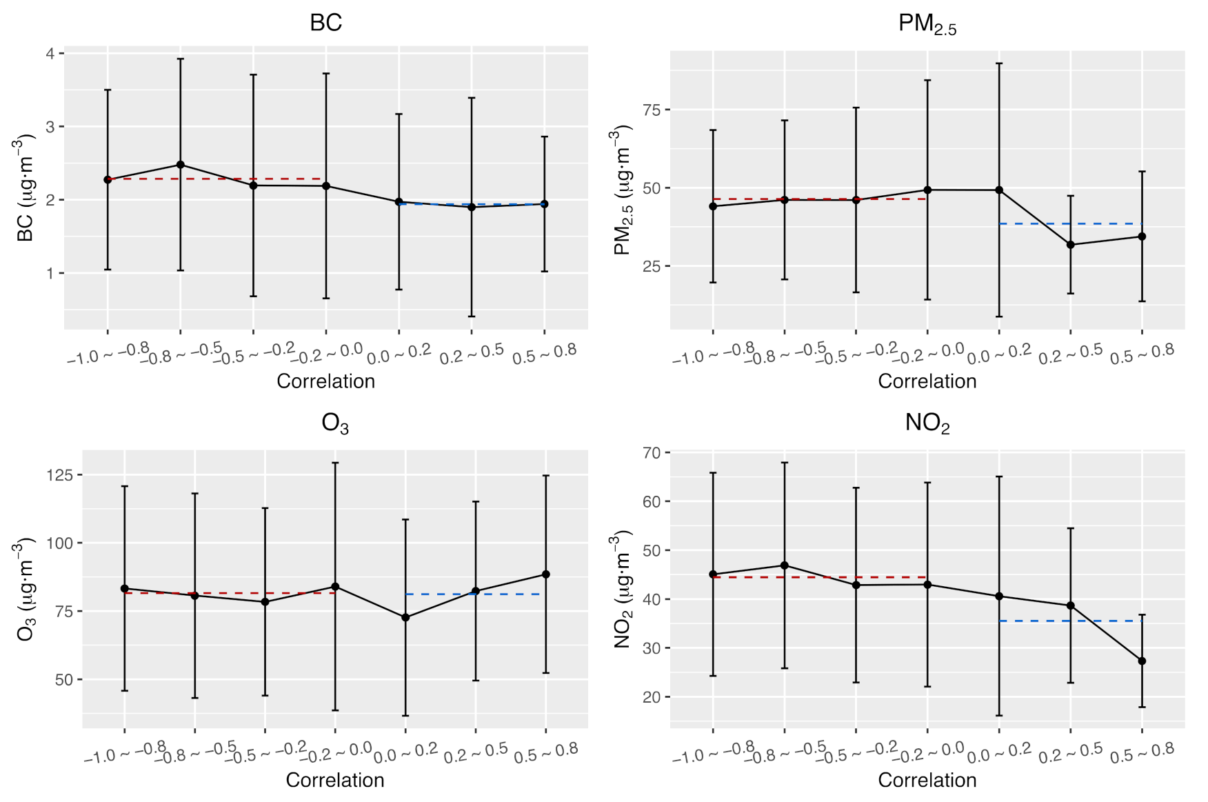
3.2. Distribution of Pollutants under Different Levels of CBO

According to Figure 5, the distribution of PM2.5, BC, O3 and NO2 varied greatly under different CBOs. In the condition of positive CBO, the average mass concentrations of BC, PM2.5 and NO2 were 1.94, 38.51 and 35.52 μg∙m−3, respectively, and those on the occasion of negative CBO were significantly lower: 2.28, 46.38 and 44.44 μg∙m−3, respectively. The average mass concentration of ozone was very close for negative CBO (81.56 μg∙m−3) and positive CBO (81.14 μg∙m−3). It is worth noting that when CBO was above 0.2, the surface ozone began to rise significantly, with PM2.5 and NO2 decreasing significantly and BC stable. According to Figure S1, the distribution of SO2, PM10, CO and meteorological elements varied greatly under different CBOs, too.

3.3. Diurnal Variations of Pollutants Concentrations and Metrological Elements under Significantly Positive and Negative CBOs

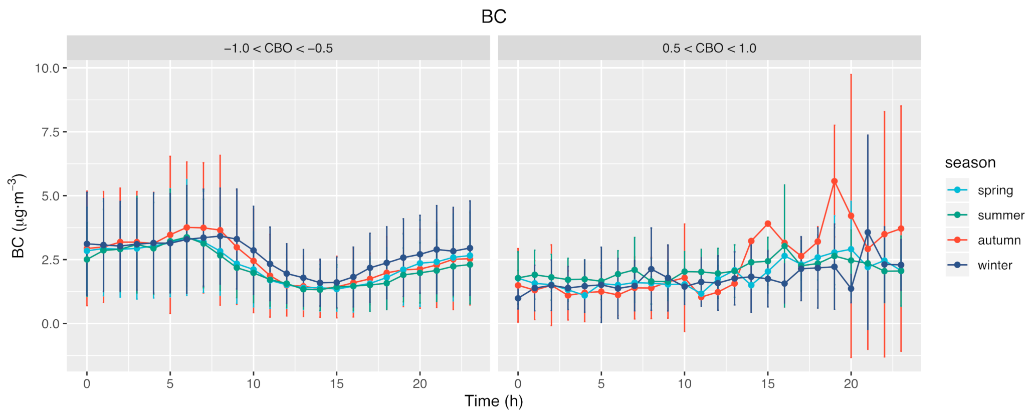
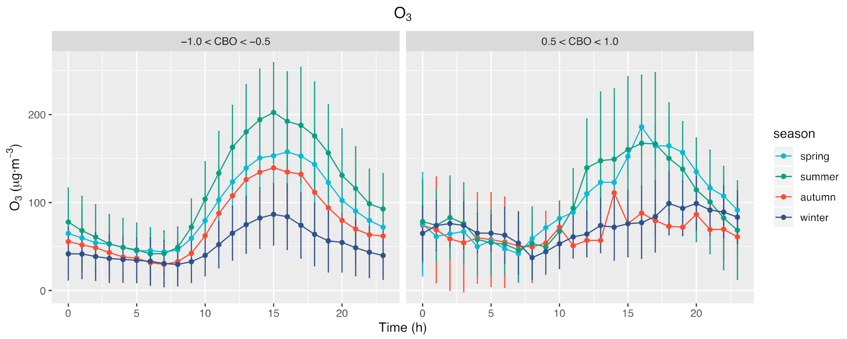
3.3.1. Diurnal Variations of BC and Ozone

There are tremendous differences of diurnal variations of BC and ozone between significantly positive CBO and negative CBO:
As for BC (Figure 6), (1) while −1.0 < CBO < −0.5, the diurnal variations of BC concentrations showed a double peak pattern. BC rose slightly around the level of 3.0 μg∙m−3 during 0:00 to 5:00 and rapidly after sunrise, reaching the first peak at round 7:00–8:00, which were 3.36, 3.37, 3.75 and 3.41 μg∙m−3 in spring, summer, autumn and winter, respectively. BC bottomed out to be around 1.40 μg∙m−3 at about 14:00, and afterwards, it began to increase and was approaching a steady value at dust. This coordinates with the results of most previous studies carried out in many regions [20,34,35,36]. (2) In contrast, while 0.5 < CBO < 1.0, mass concentration of BC was stable during 0:00–13:00, fluctuating slightly around 1.40 μg∙m−3, which was merely half of that (3.0 μg∙m−3) during the contemporaneous period of the counterpart situation. The trend of BC after 13:00 differed significantly in different seasons: In spring and summer BC rose slightly, reaching a slight peak of 2.64, 3.03 μg∙m−3 at dusk, similar to that during the contemporaneous period of the counterpart situation. In autumn, BC increased rapidly after 13:00 and reached the highest level (5.57 μg∙m−3) of the whole day at 19:00. In winter, BC rose slowly overall and saw a sudden drop at 16:00 and 20:00, and a sudden increase at 21:00.
As for O3 (Figure 7), (1) while −1.0 < CBO < −0.5, the diurnal variations of O3 concentrations showed a single peak pattern, which coordinated with the results from previous studies. O3 reached the peak at 15:00–16:00, which was 157.67, 202.46, 139.53, 86.62 μg∙m−3 in spring, summer, autumn and winter, respectively. (2) In contrast, while 0.5 < CBO < 1.0, the peak was 186.00, 167.40, 111.00 and 99.00 μg∙m−3 in spring, summer, autumn and winter, respectively, about 118.0%, 82.7%, 79.6% and 114.3% of that for −1.0 < CBO < −0.5. The maximums in summer and autumn declined obviously compared with those for −1.0 < CBO < −0.5, while the maximums in spring and winter increased obviously compared with those for −1.0 < CBO < −0.5. It is noticeable that comparing both occasions, O3 in autumn differed greatly—the mass concentration of O3 during 11:00–19:00 for 0.5 < CBO < 1.0 was obviously lower that for −1.0 < CBO < −0.5, which may be due to the increased BC during the contemporaneous period in autumn.

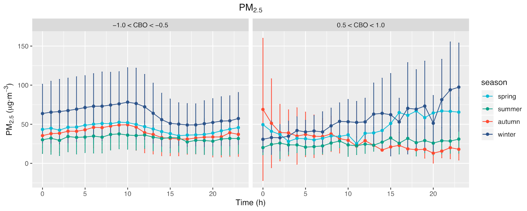
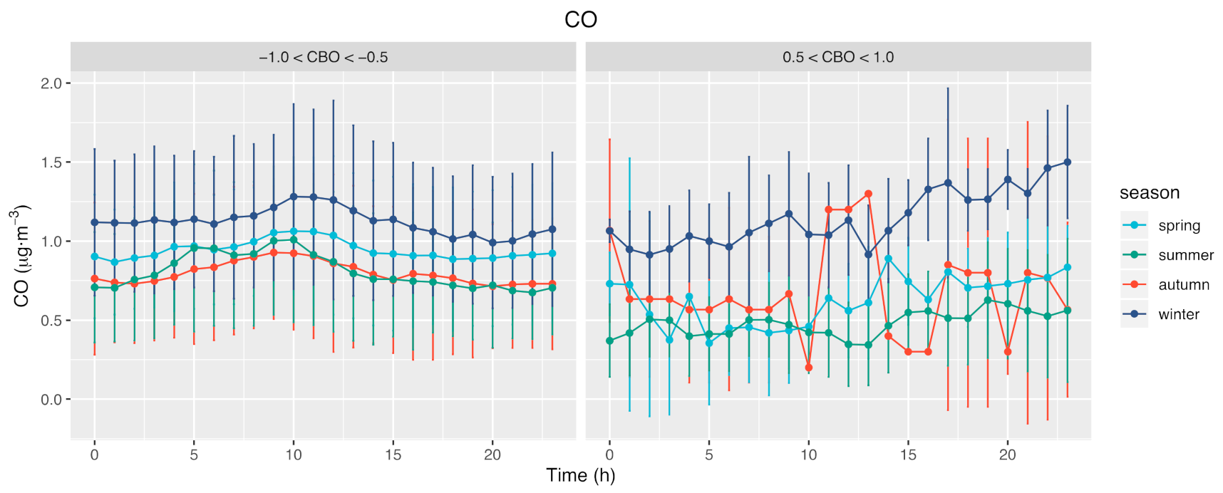
3.3.2. Diurnal Variations of the Other Pollutants

As for PM2.5 (Figure 8), (1) while −1.0 < CBO < −0.5, PM2.5 reached the peak at 9:00–10:00, which was 52.59, 36.69 and 49.43, 78.27 μg∙m−3 in spring, summer, autumn and winter, respectively. PM2.5 was severer in winter than in the other seasons. Another feature of the diurnal variations of PM2.5 in winter is that it faced a strong reduction rate (approximately 6.88 μg∙m−3∙h−1) between 11:00 and 14:00 after peaking at 9:00–10:00 and it remained at a relatively low value after 15:00. In contrast, PM2.5 in the other three seasons showed similar trends as in winter, but the change was not so dramatic. (2) In contrast, while 0.5 < CBO < 1.0, the diurnal variations of PM2.5 concentrations in spring and winter showed a different trend from that for −1.0 < CBO < −0.5. It is noticeable that PM2.5 showed a continuous rising trend, especially after 11:00, different form the declining trend of PM2.5 for −1.0 < CBO < −0.5. Thus, PM2.5 peaked in spring at 67.00 μg∙m−3 at 18:00, and in winter at 97.50 μg∙m−3 at 23:00.
As for NO2 (Figure 9), (1) while −1.0 < CBO < −0.5, the average NO2 was the highest in winter (53.34 μg∙m−3), and the lowest in summer (33.74 μg∙m−3), and the diurnal variations of NO2 had a trough between 10:00 and 19:00. (2) In contrast, while 0.5 < CBO < 1.0, the average NO2 was the highest in spring (35.85 μg∙m−3), and the lowest in winter (20.50 μg∙m−3). Overall, the NO2 concentration for 0.5 < CBO < 1.0 was lower than that for −1.0 < CBO < −0.5, and especially in winter, NO2 was merely 38.4% of that for −1.0 < CBO < −0.5. Another feather is that for all four seasons, while 0.5 < CBO < 1.0, NO2 fluctuated at a certain level instead of showing any apparent troughs throughout the day.
As shown in Figure 10, In both cases (−1.0 < CBO < −0.5 and 0.5 < CBO < 1.0), the difference in SO2 mass concentrations was not significant, and in winter, SO2 was slightly lower for −1.0 < CBO < −0.5 than for 0.5 < CBO < 1.0.
As for CO (Figure 11), (1) while −1.0 < CBO < −0.5, the diurnal variations of CO concentrations showed a single peak pattern, peaking at around 10:00–11:00. Compared with the other seasons, CO in winter was the highest on average (1.12 μg∙m−3). (2) While 0.5 < CBO < 1.0, CO concentration was also the highest on average in winter (1.14 μg∙m−3), and CO in spring and summer was slightly lower than that for −1.0 < CBO < −0.5. As for the diurnal variations, while 0.5 < CBO < 1.0, CO did not show the single peak pattern as was shown while −1.0 < CBO < −0.5. CO was overall higher during 15:00–23:00 than 0:00–14:00.

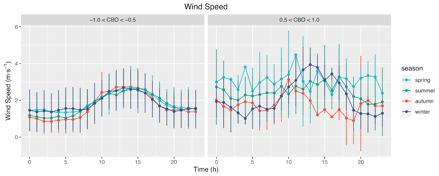
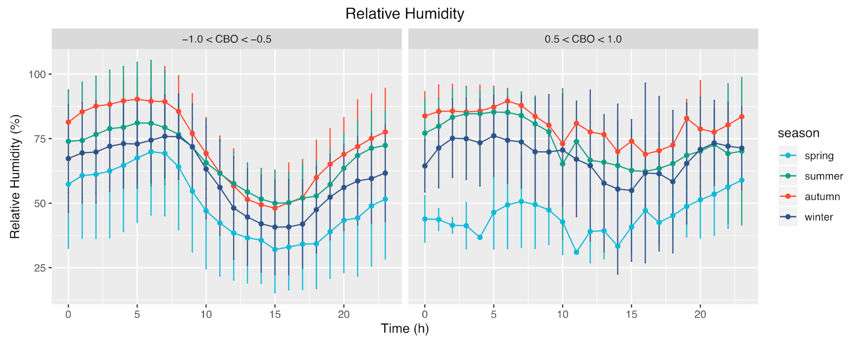
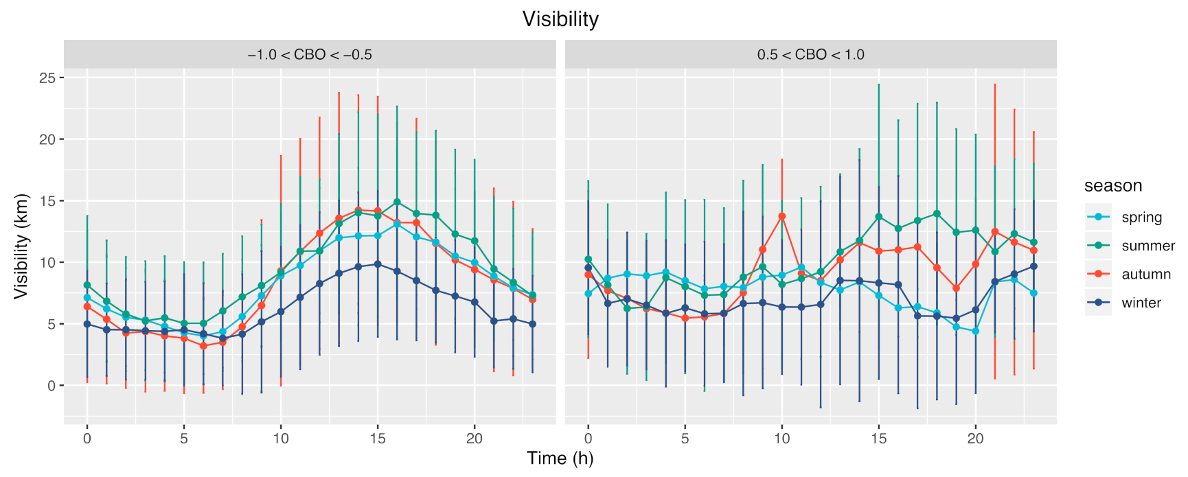
3.3.3. Diurnal Variations of Meteorological Elements

Recent research studies have studied the effects of meteorological elements on the formation of O3 with WRF-CMAQ model. One of these research studies has found that, among a series of meteorological elements, the change of wind speed had the most significant effect on the maximum daily 8 h average (MDA8) O3 [13]. In this research, the average value and the diurnal variations of wind speed differed under different CBOs. As is shown in Figure 12, (1) while −1.0 < CBO < −0.5, wind speed showed a single peak pattern, reaching a peak (around 2.68 m∙s−1) at round 14:00. In such a situation, the seasonal differences of diurnal variations of wind speed were not obvious, except for the wind speed during 0:00–8:00 (spring ≈ winter > summer > autumn). (2) While 0.5 < CBO < 1.0, the overall average wind speed was 2.13 m∙s−1, which was 15% higher than that (1.85 m∙s−1) for −1.0 < CBO < −0.5. While 0.5 < CBO < 1.0, the seasonal differences of wind speed were obvious. The diurnal variations in autumn and winter showed apparent single peak pattern as −1.0 < CBO < −0.5, while the peak happened in advance (around 10:00). The peaking values in autumn and winter were both higher than those for −1.0 < CBO < −0.5 and especially, the highest wind speed in winter (3.95 m∙s−1) was 50% higher than that (2.69 m∙s−1) for −1.0 < CBO < −0.5. Conversely, the diurnal variations in spring and summer did not show apparent single peak pattern as −1.0 < CBO < −0.5 and fluctuated widely at a relatively high level (spring: 3.10 m∙s−1, summer: 2.46 m∙s−1).
Apart from wind speed, relative humidity differed in two situations. As shown in Figure 13, (1) while −1.0 < CBO < −0.5, diurnal variations of relative humidity (RH) rose at 0:00–6:00, 15:00–23:00 and dropped at 6:00–15:00, reaching a minimum at around 15:00. The minimum was 32.04%, 49.99%, 48.07% and 40.74% in spring, summer, autumn and winter, respectively. (2) While 0.5 < CBO < 1.0, except for spring, the diurnal variations of RH in the other three seasons showed the similar pattern as −1.0 < CBO < −0.5, but the minimums (62.29% in spring, 69.00% in autumn, 54.95% in winter) were much higher than those for −1.0 < CBO < −0.5. While 0.5 < CBO < 1.0, the amplitude of diurnal variations of RH was smaller, which means RH was more stable. The most apparent difference between the two situations was in spring. The minimum RH in spring was merely 31.02%, lower than that for −1.0 < CBO < −0.5. What is more, the average RH (63.19%) during 0:00–9:00 in spring was much lower than that (45.04%) for −1.0 < CBO < −0.5.
Compared with wind speed and RH, the differences of visibility between two situations were relatively small. As shown in Figure 14, (1) while −1.0 < CBO < −0.5, diurnal variations of visibility showed a single peak pattern, reaching the maximum at around 16:00 in spring (13.10 km) and summer (14.90 km), and around 14:00–15:00 in autumn (14.22 km) and winter (9.85 km). The average visibility was the highest in summer, second in spring and autumn, and the lowest in winter. (2) While 0.5 < CBO < 1.0, the amplitude of diurnal variations of visibility was smaller than that for −1.0 < CBO < −0.5. Especially in spring and winter, visibility fluctuated at the level of around 8 km with an aptitude of about 1 km/h.

4. Conclusions

This study utilized the data of pollutant concentrations (BC, O3, PM2.5, PM10, CO, NO2 and SO2) and meteorological elements during 2015 to 2018 in Nanjing, China to analyze the daily correlation between black carbon and ozone (CBO). Samples (6988) with significantly negative CBO collected are much more than those (403) with significant positive CBO. However, the frequency analysis of CBO showed that the proportion of high positive CBO had been increasing annually, with an average increasing rate of 7.1%/year. The proportion of significantly positive CBO (0.5 < CBO < 0.8) in summer was 38.7% on average, nearly twice of that in the other seasons (19.2%). The analysis of the distribution of the pollutant concentrations under different levels of CBO showed that the average BC, PM2.5 and NO2 concentrations under positive CBO were lower than those under negative CBO. However, the difference of average ozone concentrations between such two situations was not apparent. It is noticeable that the surface ozone began to ascend when CBO was up to 0.2, with PM2.5 and NO2 decreasing and BC steady.
Besides, the diurnal variations of pollutant concentrations and meteorological elements between two situations were also compared. Under negative CBO, pollutant concentrations and meteorological elements showed obvious modes of diurnal variations: BC showed a double-peak pattern, surface ozone, PM2.5, SO2 and CO showed single-peak patterns and NO2 showed a trough from 10:00 to 19:00. Wind speed and visibility showed a single-peak pattern with little seasonal difference. Relative humidity rose first, then lowered and then rose. While under positive CBO, the above patterns of diurnal variations became less obvious and some of them even showed no patterns, but just fluctuated at a certain level. Under positive CBO, BC was stable during 0:00–13:00, fluctuating slightly around 1.40 μg∙m−3, which was merely half of that (3.0 μg∙m−3) during the contemporaneous period under negative CBO and the trend after 13:00 differed significantly in different seasons. Under negative CBO, the peaks of O3 in summer and autumn declined obviously and those in spring and winter increased obviously compared with those under negative CBO. Besides, the overall NO2 concentrations were lower and the overall wind speed was higher under positive CBO. The diurnal fluctuation of relative humidity and visibility was smaller under positive CBO.

Supplementary Materials

The following are available online at https://0-www-mdpi-com.brum.beds.ac.uk/article/10.3390/atmos12050626/s1, Figure S1: Mass concentrations of pollutants (SO2, PM10, CO) and meteorological elements (Visibility, Relative Humidity, Wind Speed) under different levels of CBO.

Author Contributions

Conceptualization, Y.T., D.Z., H.W. and B.Z.; data curation, D.Z., A.L. and S.S.; formal analysis, Y.T.; methodology, Y.T.; supervision, H.W. and B.Z.; writing—original draft, Y.T.; writing—review and editing, Y.T., H.W., D.B., A.L., S.S. and Q.D. All authors have read and agreed to the published version of the manuscript.

Funding

This research was funded by the National Key Research and Development Program of China, grant number 2016YFA0602001, the National Natural Science Foundation of China, grant number 41805096 and the China Postdoctoral Science Foundation, grant number 2018M640169.

Institutional Review Board Statement

Not applicable.

Informed Consent Statement

Not applicable.

Data Availability Statement

The ground observation data are available from the authors upon request.

Conflicts of Interest

The authors declare no conflict of interest.

References

  1. Hvidtfeldt, U.A.; Sørensen, M.; Geels, C.; Ketzel, M.; Khan, J.; Tjønneland, A.; Overvad, K.; Brandt, J.; Raaschou-Nielsen, O. Long-term residential exposure to PM2.5, PM10, black carbon, NO2, and ozone and mortality in a Danish cohort. Environ. Int. 2019, 123, 265–272. [Google Scholar] [CrossRef] [PubMed]
  2. Wang, Y.; Wild, O.; Chen, X.; Wu, Q.; Gao, M.; Chen, H.; Qi, Y.; Wang, Z. Health impacts of long-term ozone exposure in China over 2013–2017. Environ. Int. 2020, 144, 106030. [Google Scholar] [CrossRef]
  3. Mahmood, F.; Khokhar, M.F.; Mahmood, Z. Examining the relationship of tropospheric ozone and climate change on crop productivity using the multivariate panel data techniques. J. Environ. Manag. 2020, 272, 111024. [Google Scholar] [CrossRef]
  4. de Foy, B.; Brune, W.H.; Schauer, J.J. Changes in ozone photochemical regime in Fresno, California from 1994 to 2018 deduced from changes in the weekend effect. Environ. Pollut. 2020, 263, 114380. [Google Scholar] [CrossRef]
  5. Jenkin, M.E.; Derwent, R.G.; Wallington, T.J. Photochemical ozone creation potentials for volatile organic compounds: Rationalization and estimation. Atmos. Environ. 2017, 163, 128–137. [Google Scholar] [CrossRef]
  6. Robinson, J.; Kotsakis, A.; Santos, F.; Swap, R.; Knowland, K.E.; Labow, G.; Connors, V.; Tzortziou, M.; Abuhassan, N.; Tiefengraber, M.; et al. Using networked Pandora observations to capture spatiotemporal changes in total column ozone associated with stratosphere-to-troposphere transport. Atmos. Res. 2020, 238, 104872. [Google Scholar] [CrossRef]
  7. Tarasick, D.W.; Carey-Smith, T.K.; Hocking, W.K.; Moeini, O.; He, H.; Liu, J.; Osman, M.K.; Thompson, A.M.; Johnson, B.J.; Oltmans, S.J.; et al. Quantifying stratosphere-troposphere transport of ozone using balloon-borne ozonesondes, radar windprofilers and trajectory models. Atmos. Environ. 2019, 198, 496–509. [Google Scholar] [CrossRef]
  8. Farooqui, Z.M.; John, K.; Biswas, J.; Sule, N. Modeling analysis of the impact of anthropogenic emission sources on ozone concentration over selected urban areas in Texas. Atmos. Pollut. Res. 2013, 4, 33–42. [Google Scholar] [CrossRef] [Green Version]
  9. Im, U.; Poupkou, A.; Incecik, S.; Markakis, K.; Kindap, T.; Unal, A.; Melas, D.; Yenigun, O.; Topcu, S.; Odman, M.T.; et al. The impact of anthropogenic and biogenic emissions on surface ozone concentrations in Istanbul. Sci. Total Environ. 2011, 409, 1255–1265. [Google Scholar] [CrossRef]
  10. Liu, P.; Song, H.; Wang, T.; Wang, F.; Li, X.; Miao, C.; Zhao, H. Effects of meteorological conditions and anthropogenic precursors on ground-level ozone concentrations in Chinese cities. Environ. Pollut. 2020, 262, 114366. [Google Scholar] [CrossRef]
  11. Ryu, Y.-H.; Baik, J.-J.; Lee, S.-H. Effects of anthropogenic heat on ozone air quality in a megacity. Atmos. Environ. 2013, 80, 20–30. [Google Scholar] [CrossRef]
  12. Ma, Y.; Ma, B.; Jiao, H.; Zhang, Y.; Xin, J.; Yu, Z. An analysis of the effects of weather and air pollution on tropospheric ozone using a generalized additive model in Western China: Lanzhou, Gansu. Atmos. Environ. 2020, 224, 117342. [Google Scholar] [CrossRef]
  13. Liu, Y.; Wang, T. Worsening urban ozone pollution in China from 2013 to 2017—Part 1: The complex and varying roles of meteorology. Atmos. Chem. Phys. 2020, 20, 6305–6321. [Google Scholar] [CrossRef]
  14. Bond, T.C.; Doherty, S.J.; Fahey, D.W.; Forster, P.M.; Berntsen, T.; DeAngelo, B.J.; Flanner, M.G.; Ghan, S.; Kärcher, B.; Koch, D.; et al. Bounding the role of black carbon in the climate system: A scientific assessment: Black Carbon in the Climate System. J. Geophys. Res. Atmos. 2013, 118, 5380–5552. [Google Scholar] [CrossRef]
  15. Pani, S.K.; Wang, S.-H.; Lin, N.-H.; Chantara, S.; Lee, C.-T.; Thepnuan, D. Black carbon over an urban atmosphere in northern peninsular Southeast Asia: Characteristics, source apportionment, and associated health risks. Environ. Pollut. 2020, 259, 113871. [Google Scholar] [CrossRef]
  16. Lin, W.; Dai, J.; Liu, R.; Zhai, Y.; Yue, D.; Hu, Q. Integrated assessment of health risk and climate effects of black carbon in the Pearl River Delta region, China. Environ. Res. 2019, 176, 108522. [Google Scholar] [CrossRef] [PubMed]
  17. Gu, Y.; Zhang, W.; Yang, Y.; Wang, C.; Streets, D.G.; Yim, S.H.L. Assessing outdoor air quality and public health impact attributable to residential black carbon emissions in rural China. Resour. Conserv. Recycl. 2020, 159, 104812. [Google Scholar] [CrossRef]
  18. Ji, D.; Gao, W.; Maenhaut, W.; He, J.; Wang, Z.; Li, J.; Du, W.; Wang, L.; Sun, Y.; Xin, J.; et al. Impact of air pollution control measures and regional transport on carbonaceous aerosols in fine particulate matter in urban Beijing, China: Insights gained from long-term measurement. Atmos. Chem. Phys. 2019, 19, 8569–8590. [Google Scholar] [CrossRef] [Green Version]
  19. Kucbel, M.; Corsaro, A.; Švédová, B.; Raclavská, H.; Raclavský, K.; Juchelková, D. Temporal and seasonal variations of black carbon in a highly polluted European city: Apportionment of potential sources and the effect of meteorological conditions. J. Environ. Manag. 2017, 203, 1178–1189. [Google Scholar] [CrossRef]
  20. Bibi, S.; Alam, K.; Chishtie, F.; Bibi, H.; Rahman, S. Temporal variation of Black Carbon concentration using Aethalometer observations and its relationships with meteorological variables in Karachi, Pakistan. J. Atmos. Sol.-Terr. Phys. 2017, 157–158, 67–77. [Google Scholar] [CrossRef]
  21. Bai, Z.; Cui, X.; Wang, X.; Xie, H.; Chen, B. Light absorption of black carbon is doubled at Mt. Tai and typical urban area in North China. Sci. Total Environ. 2018, 635, 1144–1151. [Google Scholar] [CrossRef]
  22. Ma, Y.; Huang, C.; Jabbour, H.; Zheng, Z.; Wang, Y.; Jiang, Y.; Zhu, W.; Ge, X.; Collier, S.; Zheng, J. Mixing state and light absorption enhancement of black carbon aerosols in summertime Nanjing, China. Atmos. Environ. 2020, 222, 117141. [Google Scholar] [CrossRef]
  23. Xie, C.; Xu, W.; Wang, J.; Liu, D.; Ge, X.; Zhang, Q.; Wang, Q.; Du, W.; Zhao, J.; Zhou, W.; et al. Light absorption enhancement of black carbon in urban Beijing in summer. Atmos. Environ. 2019, 213, 499–504. [Google Scholar] [CrossRef]
  24. Zhang, B.-N.; Kim Oanh, N.T. Photochemical smog pollution in the Bangkok Metropolitan Region of Thailand in relation to O3 precursor concentrations and meteorological conditions. Atmos. Environ. 2002, 36, 4211–4222. [Google Scholar] [CrossRef]
  25. Hu, D.; Chen, Y.; Wang, Y.; Daële, V.; Idir, M.; Yu, C.; Wang, J.; Mellouki, A. Photochemical reaction playing a key role in particulate matter pollution over Central France: Insight from the aerosol optical properties. Sci. Total Environ. 2019, 657, 1074–1084. [Google Scholar] [CrossRef] [Green Version]
  26. Li, G.; Zhang, R.; Fan, J.; Tie, X. Impacts of black carbon aerosol on photolysis and ozone. J. Geophys. Res. Atmos. 2005, 110. [Google Scholar] [CrossRef] [Green Version]
  27. Gao, J.; Zhu, B.; Xiao, H.; Kang, H.; Pan, C.; Wang, D.; Wang, H. Effects of black carbon and boundary layer interaction on surface ozone in Nanjing, China. Atmos. Chem. Phys. 2018, 18, 7081–7094. [Google Scholar] [CrossRef] [Green Version]
  28. Lu, X.; Zhang, L.; Chen, Y.; Zhou, M.; Zheng, B.; Li, K.; Liu, Y.; Lin, J.; Fu, T.-M.; Zhang, Q. Exploring 2016–2017 surface ozone pollution over China: Source contributions and meteorological influences. Atmos. Chem. Phys. 2019, 19, 8339–8361. [Google Scholar] [CrossRef] [Green Version]
  29. Shen, L.; Jacob, D.J.; Liu, X.; Huang, G.; Li, K.; Liao, H.; Wang, T. An evaluation of the ability of the Ozone Monitoring Instrument (OMI) to observe boundary layer ozone pollution across China: Application to 2005–2017 ozone trends. Atmos. Chem. Phys. 2019, 19, 6551–6560. [Google Scholar] [CrossRef] [Green Version]
  30. Tan, Y.; Wang, H.; Shi, S.; Shen, L.; Zhang, C.; Zhu, B.; Guo, S.; Wu, Z.; Song, Z.; Yin, Y.; et al. Annual variations of black carbon over the Yangtze River Delta from 2015 to 2018. J. Environ. Sci. 2020, 96, 72–84. [Google Scholar] [CrossRef] [PubMed]
  31. Lu, X.; Hong, J.; Zhang, L.; Cooper, O.R.; Schultz, M.G.; Xu, X.; Wang, T.; Gao, M.; Zhao, Y.; Zhang, Y. Severe Surface Ozone Pollution in China: A Global Perspective. Environ. Sci. Technol. Lett. 2018, 5, 487–494. [Google Scholar] [CrossRef]
  32. Xie, Y.; Dai, H.; Zhang, Y.; Wu, Y.; Hanaoka, T.; Masui, T. Comparison of health and economic impacts of PM2.5 and ozone pollution in China. Environ. Int. 2019, 130, 104881. [Google Scholar] [CrossRef] [PubMed]
  33. Drinovec, L.; Močnik, G.; Zotter, P.; Prévôt, A.S.H.; Ruckstuhl, C.; Coz, E.; Rupakheti, M.; Sciare, J.; Müller, T.; Wiedensohler, A.; et al. The “dual-spot” Aethalometer: An improved measurement of aerosol black carbon with real-time loading compensation. Atmos. Meas. Tech. 2015, 8, 1965–1979. [Google Scholar] [CrossRef] [Green Version]
  34. Putero, D.; Cristofanelli, P.; Marinoni, A.; Adhikary, B.; Duchi, R.; Shrestha, S.D.; Verza, G.P.; Landi, T.C.; Calzolari, F.; Busetto, M.; et al. Seasonal variation of ozone and black carbon observed at Paknajol, an urban site in the Kathmandu Valley, Nepal. Atmos. Chem. Phys. 2015, 15, 13957–13971. [Google Scholar] [CrossRef] [Green Version]
  35. Ran, L.; Deng, Z.Z.; Wang, P.C.; Xia, X.A. Black carbon and wavelength-dependent aerosol absorption in the North China Plain based on two-year aethalometer measurements. Atmos. Environ. 2016, 142, 132–144. [Google Scholar] [CrossRef]
  36. Ravi Kiran, V.; Talukdar, S.; Venkat Ratnam, M.; Jayaraman, A. Long-term observations of black carbon aerosol over a rural location in southern peninsular India: Role of dynamics and meteorology. Atmos. Environ. 2018, 189, 264–274. [Google Scholar] [CrossRef]
Figure 1. The scatter plot and the linear fit of O3 and BC concentrations.
Atmosphere 12 00626 g001aAtmosphere 12 00626 g001b
Figure 2. The annual variations of the frequency of negative CBO and positive CBO.
Atmosphere 12 00626 g002
Figure 3. The monthly variations of the frequency of negative CBO and positive CBO.
Atmosphere 12 00626 g003
Figure 4. The seasonal variations of the frequency of negative CBO and positive CBO.
Atmosphere 12 00626 g004
Figure 5. Mass concentrations of pollutants (BC, PM2.5, O3, NO2) under different levels of CBO.
Atmosphere 12 00626 g005
Figure 6. Diurnal variations of BC in two situations: (left): −1.0 < CBO < −0.5 and (right): 0.5 < CBO < 1.0.
Atmosphere 12 00626 g006
Figure 7. Diurnal variations of O3 in two situations: (left): −1.0 < CBO < −0.5 and (right): 0.5 < CBO < 1.0.
Atmosphere 12 00626 g007
Figure 8. Diurnal variations of PM2.5 in two situations: (left): −1.0 < CBO < −0.5 and (right): 0.5 < CBO < 1.0.
Atmosphere 12 00626 g008
Figure 9. Diurnal variations of NO2 in two situations: (left): −1.0 < CBO < −0.5 and (right): 0.5 < CBO < 1.0.
Atmosphere 12 00626 g009
Figure 10. Diurnal variations of SO2 in two situations: (left): −1.0 < CBO < −0.5 and (right): 0.5 < CBO < 1.0.
Atmosphere 12 00626 g010
Figure 11. Diurnal variations of CO in two situations: (left): −1.0 < CBO < −0.5 and (right): 0.5 < CBO < 1.0.
Atmosphere 12 00626 g011
Figure 12. Diurnal variations of wind speed in two situations: (left): −1.0 < CBO < −0.5 and (right): 0.5 < CBO < 1.0.
Atmosphere 12 00626 g012
Figure 13. Diurnal variations of relative humidity in two situations: (left): −1.0 < CBO < −0.5 and (right): 0.5 < CBO < 1.0.
Atmosphere 12 00626 g013
Figure 14. Diurnal variations of visibility in two situations: (left): −1.0 < CBO < −0.5 and (right): 0.5 < CBO < 1.0.
Atmosphere 12 00626 g014
Publisher’s Note: MDPI stays neutral with regard to jurisdictional claims in published maps and institutional affiliations.

