
The 3D Neural Network for Improving Radar-Rainfall Estimation in Monsoon Climate
by
 , ,
, ,
Nurulhani Roslan
1 ,
,
Mohd Nadzri Md Reba
2,* ,
,
Syarawi M. H. Sharoni
1 and
Mohammad Shawkat Hossain
3
1
Faculty of Built Environment and Surveying (FABU), Universiti Teknologi Malaysia, Johor Bahru 81310 UTM, Johor, Malaysia
2
Geoscience and Digital Earth Centre (INSTeG), Research Institute for Sustainable and Environment (RISE), Universiti Teknologi Malaysia, Johor Bahru 81310 UTM, Johor, Malaysia
3
Institute of Oceanography and Environment (INOS), Universiti Malaysia Terengganu (UMT), Kuala Nerus 21030, Terengganu, Malaysia
*
Author to whom correspondence should be addressed.
Atmosphere 2021, 12(5), 634; https://0-doi-org.brum.beds.ac.uk/10.3390/atmos12050634
Submission received: 30 March 2021
/
Revised: 24 April 2021
/
Accepted: 28 April 2021
/
Published: 17 May 2021
(This article belongs to the Special Issue Weather Radar in Rainfall Estimation)
Abstract
:The reflectivity (Z)—rain rate (R) model has not been tested on single polarization radar for estimating monsoon rainfall in Southeast Asia, despite its widespread use for estimating heterogeneous rainfall. The artificial neural network (ANN) regression has been applied to the radar reflectivity data to estimate monsoon rainfall using parametric Z-R models. The 10-min reflectivity data recorded in Kota Bahru radar station (in Malaysia) and hourly rain record in nearby 58 gauge stations during 2013–2015 were used. The three-dimensional nearest neighbor interpolation with altitude correction was applied for pixel matching. The non-linear Levenberg Marquardt (LM) regression, integrated with ANN regression minimized the spatiotemporal variability of the proposed Z-R model. Results showed an improvement in the statistical indicator, when LM and ANN overestimated (6.6%) and underestimated (4.4%), respectively, the mean total rainfall. For all rainfall categories, the ANN model has a positive efficiency ratio of >0.2.
1. Introduction
The heterogenous of rain intensity that Southeast Asia (SEA) experiences throughout the northeast monsoon (NEM) and southwest monsoon (SWM) and transition monsoon every year, generally refers to the “monsoon rainfall”. The region often receives mean annual rainfall of more than 2500 mm/year. The NEM brings in more rainfall (37–52% of total annual rainfall) than of the SWM (33–40%) [1,2]. Worldwide most widely discussed climate phenomena such as El Niño-Southern Oscillation (ENSO) and Madden–Julian Oscillation (MJO) may be intrinsically linked with interseason variability of the downpour rain [3]. The impact of extreme rainfall events in SEA is eventually the episodes of severe floods. For instance, a massive flood event in Kelantan, Malaysia in 2014 resulted in huge economic loss about USD 0.3 million [4]. Therefore, measuring accurate, reliable, and real time rainfall is crucial in flood management and mitigation specially across SEA [1].
Traditionally used rain gauges although provide rainfall information limited by its distribution in sparse locations and they are unable to inform spatial rainfall variability [3]. Despite the fact that the satellite-based microwave-radiometer can measure the volumetric column of rainfall and spatial distribution of water vapor in the atmosphere, it is inherently limited by spatiotemporal resolution [5]. Unlike both variants, the weather radar offers continuous observations on a wider spatial coverage (~200 km), with a higher temporal resolution (~10 min). Taking advantage of weather radar, several studies have advanced the knowledge about atmospheric constituents and proposed weather forecasting techniques, as well as improved inputs for developing hydrological models [6]. Since 1978, numerous weather radar observation campaigns have been conducted in the SEA with a view to improve the accuracy of the prediction model, however, they have always been affected by the heterogenous rain, originated from the intra-seasonal, synoptic, and mesoscale precipitation processes [7].
Estimating rain from the weather radar measurement is not straightforward as the radar data are formed in a multi-dimensional structure based on the range (distance), azimuth (angle), and elevation (height) in a spherical coordinate system. The radar reflectivity, Z, measured in dBZ, is related to the raindrop size distribution (DSD) in a radar sample volume [8,9] and inverting to the rain rate, R (measured in mm/s), which strictly depends on the raindrop number and DSD. Thus, the relationship has been introduced by [10] through the parametric power–law relationship.
The α and β are the coefficients are determined empirically. Although both parameters are dependent on the climate, drop size distribution, rainfall types, and microphysical properties, they are independent to the rainfall rate itself [11]. The prefactor α is more related to the radar reflectivity, while the exponent β has a close relationship between the growth size of rain particles and size reshaping process [12]. In tropical climate, the warm air forms the DSD and the drops tend to have different sizes for a given rainfall rate with the monsoon effect. Therefore, large variation of the reflectivity requires a revision on the Z-R relationship in the study area.
So far, three methods have been reported to present such relationship: (a) drop size distribution [13], (b) matching probability [14], and (c) statistical technique [15]. The first technique uses disdrometer to link with the rain rate, yet it is not widely used due to higher cost and highly competent operator requirement, particularly in the SEA. The second approach matches the same cumulative distribution function of grid reflectivity and gauge vector. However, this approach does not represent the individual rain rate and is sensitive to higher reflectivity. The last technique implemented a parametric model for deriving the regression coefficients (α and β in Z-R model) or non-parametric statistical form which is more efficient in inverting results but demands massive input data. Even the third technique is the simplest one, it has likelihood to errors when incorporating the exact volume and height in the atmosphere for the rain gauge measurements.
Marshall–Palmer (MP) and Rosenfeld (ROS) regression coefficients (giving α = 200 and β = 1.6 and α = 250 and β = 1.2, respectively) have been widely applied in many regions [16,17], but are less robust for the regions where rain pattern and intensity during monsoon is heterogenous. The default MP model has an overestimation of about 80%, resulting in a cumulative estimate of about 160 mm/h [17,18]. This approach requires a priori knowledge of the coefficients in order to initiate the MP model. The model overestimation was also found in other studies, such as 30% in [19] and 50% in [20], respectively. The empirical technique has shown much improvement for monsoon rainfall if the spatial bias adjustment is applied after the coefficients were determined [16,21]. Radiometric correction resulted from bias adjustment has been reviewed comprehensively in many studies in Europe, but less documented in SEA [22]. Although the research focused on the parametric Z-R model, improving the accuracy has least considered in the past. The appropriate processing steps in different monsoon rainfall classes may increase the estimation accuracy [23,24].
Radiometric bias occurs when surface rainfall measurement obtained from the gauge is used to match with the hypothetically volumetric rainfall derived from the radar reflectivity. The correlation may deteriorate if the pixel reflectivity is either exceptionally low (0 dBZ) or high (more than 70 dBZ). Therefore, pixel matching in radar calibration is crucial for minimizing the radiometric bias at different spatial and temporal conditions. The bias could be as high as 76% [25], thus deteriorating the Z-R model correlation [14]. Probability matching method (PMM) [26], window probability matching method (WPMM) [27], window correlation matching method (WCMM) [28], and region probability matching method (RPMM) [14] have been used in pixel matching for more than two decades. The PMM provided a weak correlation coefficient, while the RPMM was not robust for rains with higher temporal variability [14]. Even the WCMM was designed to minimize spatiotemporal variations, however, failed to provide accurate and reliable areal rainfall estimation.
This study assumed that, unlike the parametric Z-R model, the non-parametric model such as artificial neural network (ANN), could be an alternative to provide better monsoon rainfall estimation from the weather radar [29]. The method can be more robust and plausible for non-linear mapping and error-tolerant regression in all radar rainfall applications [30,31]. The ANN inverts the radar reflectivity to the rain rate by means of the bias and weight vector in the generalization model. Thus, no spatial bias adjustment needs to be applied. Yet, this approach requires extensive training samples to correlate the radar reflectivity with the rain gauge data [32]. Besides, it is time-consuming since the user has to retrain the training network repeatedly until a high correlation is achieved by the network [33]. The ANN regression was initiated by [34] using radial basis function neural network (RBFNN) and this effort continues using the backpropagation feed-forward neural network (BPNN) [35] for weather radar rainfall estimation. The RBFANN consists of neurons input vector and a radial basis layer to produce linear output using few numbers of hidden layer. The BPANN is part of a feed-forward neural network (FFNN) with all datasets flow in one direction and have a feedback known as weight to produce the output. The FFNN is the simplest network where the information moved in one direction without any looping. These studies discussed different criteria for network input with appropriate training and validation data, as well as the number of hidden neurons involved.
However, the ANN technique has not been tested for monsoon rainfall, especially in the context of the climate in Malaysia. This study therefore presents a framework for estimating monsoon rainfall using parametric Z-R models and ANN regression on the reflectivity data obtained from the single polarization radar in Malaysia. The framework shows a clear contrast between the two models and, thus, this paper aims to assess the accuracy of the monsoon rainfall estimates. Section 2 introduces the study area and related data used for this study. Section 3 describes the framework to accurately estimate the monsoon rainfall from the reflectivity data in which the geometric and radiometric correction in pixel matching, the non-linear Z-R model with spatial field bias adjustment and the ANN regression are presented in this paper.
2. Materials and Methods
2.1. Study Area and Data
Radar reflectivity data were collected by the S-band (10.91 cm) single-horizontal polarization Doppler radar at Kota Bahru, Kelantan, and the data are under custodian of the Malaysia Meteorological Department (MMD). The radar was stationed at 13 m ASL and it covers radial measurement from 50 to 250 km radii (Figure 1).
This area experiences the wet and humid tropical climate throughout the year with an average rain record of 3689 mm/year. More information of the study area is discussed in [36]. The Kelantan river covers the basin in 284 km length which consists of Golok River Basin, Kemasin River Basin, Semerak River Basin, and Kelantan River Basin.
The reflectivity data have a spatial resolution of 0.8 km and 10 min temporal sampling. The reflectivity data representing the return signal were sampled in the lowest scanning angle of 0.7 degree at the position within 2-km altitude from the ground. Such setup would reduce the ground clutter effect which is typically pronounced in the signal received close to the radar antenna providing reliable rainfall information near to the surface [37]. Calibration through the threshold log receiver of signal-to-noise ratio (LOG) and the Doppler channel clutter-to-signal ratio (CSR) were applied in pre-processing in IRIS software for minimizing the uncertainties [38]. System calibration is also being applied during regular maintenance routine in every six months. No correction on the radar signal attenuation is conducted [39]. The reflectivity data obtained during the wet season of the NEM from 2013 to 2015 (January, February, March, September, October, November, and December) and recorded in the SIGMET file format. General specifications of Kota Bahru radar are listed in Table 1.
Rain gauge measurement by network of tipping bucket gauges provide rain intensity at a volumetric resolution of 0.2 mm in 1-h resolution and this routine is organized by the Department of Irrigation and Drainage (DID). There are 58 gauges involved in the 200-km radar observation range (Figure 1) where 29, 16, and 13 gauges in the near (4 to 50 km), intermediate (51 to 100 km), and far (101 to 200 km) range from the radar station, respectively. Many gauges are stationed in flat area (Northern part) but sparsely distributed on high terrains in the south of Kelantan and they are mostly located along the river. Data quality control and homogeneity test have been conducted on all rain gauges in Kelantan [40,41]. These studies reported that 50 gauges have experienced more than 10% of data void and 41 gauges were working in homogenous fashion while the rest of gauges were doubtful.
The digital elevation model (DEM) data are a product of the Shuttle Radar Topography Mission (SRTM) with 30 m (1 arc-second) pixel spacing and was used for altitude correction of each rain gauge. The data have spatial resolution of 30 m and 90 m in vertical and horizontal, respectively [42]. The DEM products have been corrected on the void pixels which can be downloaded from the U.S. Geological Survey (USGS) website.
2.2. Data Preparation
The radar data conversion was applied through an open-source software, namely Python atmospheric radiation measurement (ARM) radar toolkit (Py-ART) [43] to generate the NetCDF from the SIGMET files to ensure interoperability for reading and processing the reflectivity data. The 10-min reflectivity data are integrated in 1-h measurement to temporally match with the gauge data. The reflectivity data with Z ≤ 0 dBZ were removed to avoid misinterpretation of raindrop target representing such measurement and thus underestimating the rain estimates. The rain data from gauge measurement below 0.3 mm/h were eliminated to avoid false measurement for low-intensity rainfall as suggested by [44], where the zero rain rate decreases the spatial variability of rainfall and significantly affects the correlation in high rainfall intensity. As a result, about 9860 of hourly reflectivity data were generated and matched with the gauge observation time.
2.3. Geometric Transformation and Pixel Matching
The reflectivity data have scattered reflectivity attributes in spherical coordinate system and therefore it should be converted to the local map projection presenting in real earth coordinates to match with the gauge location. The geometric transformation was applied in MATLAB and the original coordinate was in polar system and transformed into the Cartesian coordinate system, as shown in Figure 2. The coordinate transformation algorithm adopted from [12,45] is used by incorporating the effective earth radius factor 4/3 as an input.
The geometric correction only determines the planimetric and height position but the corresponding reflectivity estimate was always not defined [46]. Therefore, resampling of the reflectivity pixel has to be conducted. The three-dimensional pixel interpolation based on the nearest neighbor (NN) was used and the Cartesian derived coordinates of reflectivity and the corresponding gauge as the inputs with the height correction of gauge as in Equation (1).
where, is the rain gauge altitude determined from the DEM (meter) and indicates the altitude of the radar station (meter). Despite of the fact that many interpolation methods have been introduced in geometric correction of radar data [47,48,49,50], most of them only operate in the 2D Cartesian grid. The nearest neighbor is the simplest interpolation which preserves the reflectivity in a grid more than of other interpolation and producing less artificial reflectivity estimate [51]. Study by [49] stated that the NN worked well for the lowest elevation angle in radar rainfall estimates. At this point, the position of reflectivity pixel is almost matched with the position of gauge data and the total samples are about 45,240.
2.4. Rainfall Intensity Classification
To sustain the quality of reflectivity, the match samples fall in the measurement range between 4 to 50 km were used because the correlation to the gauge is more than 0.4 and more than 80% of gauge stations were included. For adequate assessment of the spatiotemporal variability, all measurement data were sorted in three different intensity classes namely low rain (0.3 ≤ R < 3.2 mm/h), medium rain (3.2 ≤ R < 13 mm/h), and high rain (R ≥ 13 mm/h). This study assumes that the intensity cohort creates the optimum way for assessment in controllable sample. Studies by [52,53] have proved that by partitioning the sample in low rainfall rate has reduced the estimation uncertainty and recommend this routine in estimating the monsoon rainfall particularly with highly heterogenous rain types. There are about 3257 samples were selected at this point.
2.5. Non-Linear Least Square Optimization in Z-R Modeling
Parametric Z-R models have been derived either in linear or non-linear regression models depending on the quality of both data and data screening [54,55]. In this study, the non-linear regression with the Levenberg Marquardt (LM) optimization [56] is chosen to estimate the optimal pre-factor α and exponent β in the Z-R model. Some conditional functions such as the minimum cost function must meet within the given constraint of the α and β (200 < α < 600 and 1.2 < β < 1.8) and the functional tolerance of 50% are applied. The method applies functional weight and parametric conditions (different rain intensity classes) in the objective function. The LM method was merely considered because of this method shows more robustness in the prediction of the targeted parameter (rain rate) even though the initial value of that parameter was far from the corresponding reflectivity. Besides, the LM also has better time-efficiency in the inversion processing. This study reapplies the coefficients derived in [36] to initiate the intensity-based Z-R regression.
To minimize the difference induced by the spatial bias inherited in interpolated reflectivity pixels [6], the mean-field bias (MFB) known by gauge to radar ratio (G/R) [22] is applied, right after both coefficients were determined.
where is the accumulated rainfall (mm/h) at the gauge i and is the accumulated radar rainfall estimates (mm/h) at the gauge i, and N is the total number of the matching pair of those two observations. The bias factor, B is typically applied on the derived Z-R model with the prefactor α and coefficient β as follows [21,57].
At this point, 1952 samples were applied in model development while 1305 for validation.
2.6. Artificial Neural Network (ANN) Regression Model
The artificial neural network (ANN) training network aims to prepare more comprehensive model that adapts to possible rain condition and spatio-temporal variability of radar reflectivity in regard to season, location, climate, and the SNR. The network is designed with three-layer perceptron consists of two hidden layers in a network, as suggested in [34]. The network requires input of the reflectivity data and the target vector of the rain rate at the gauge. The hidden layer is used to increase the non-linearity relation and transform the representation of reflectivity data for better generalization over the function. For the development of the ANN model, three datasets are considered, which are training, testing, and validation. The training dataset used to determine the model’s weight and the testing dataset was used to test the performance of the trained model to predict the target vector (rainfall from the gauge). Meanwhile, the validation was used to ensure that the model is accurate and efficient to train independent reflectivity data. In this study, 60% and 40% of the match sample of reflectivity and gauge data was divided for training network and validation process that corresponds to 1952 and 1305 samples, respectively.
The Bayesian regularization method was assigned as the training algorithm and the backpropagation feed-forward neural network (BPANN), in a log sigmoid layer was chosen to develop radar inversion model and thus estimate the radar rainfall. The network fitting general equation is shown in Equation (4).
where is the rainfall estimates from the radar (mm/h), n is the number of the layer in the training network, is the transfer function, is the neuron weight and in the bias of the neuron. The main objective is to find a network function of inversed radar, learn the reflectivity value pattern in the input vector and produce the best function approximation to the target (i.e., the ‘true’ rain gauge measurement). The training network will stop when it reaches the minimum MSE and higher correlation coefficient (i.e., MSE less than 0.2 and Rc larger than 0.7).
In order to define the impact of different rain intensity in ANN model, samples in low, medium and high rain classes and whole classes are used at separate training networks. There are about 1436, 390, and 126 samples applied in each abovementioned training network, respectively. In the validation process, the derived ANN model was applied on the remaining 30% of match samples to assess the ANN accuracy. The validation was conducted on the abovementioned training networks and involved about 958, 262, and 85 samples for low, medium, and high rain classes and 1305 for whole samples, respectively.
2.7. Accuracy Assessment
All derived rainfall from the reflectivity data from MP, ROS, LM, and ANN are quantitatively assessed using the correlation (R), coefficient of determination (R2), root mean square error (RMSE), bias, and Nash- Sutcliffe efficiency index (NSE) [21,58] as follows.
where is the radar rainfall estimate (mm), is the rain rate measurement from the rain gauge (mm), represents the average of the rainfall at the gauge [mm], n is the number of the sample. Basically, the range of R is between −1 to 1 where the positive value indicates the relationship between the reflectivity and the gauge data are mutually established and vice versa. The RMSE indicates the error represents the average deviation between the radar rainfall estimates from the rain gauge. The lower RMSE stipulates that the radar estimate has a strong tendency to the rain gauge. The NSE gives result from to 1 where an index closer to 1 is a perfect score, negative index efficiency represents the average of the actual rain gauge measurement performing better than the predicted rainfall of the new Z-R model, while 0 indicates that the accuracy of the average between the rain gauge and radar rain rate are equal.
To comprehensively assess the quality of the parametric and non-parametric models, the Taylor diagram (TD) was presented in which the results of R, RMSE, and SIGMA [59]. The expression is as follows:
where, E′ represents the centered RMSE between the fields, and and are the variances of the model and rain gauge. The diagram has been used to analyze proximity of the radar rainfall estimate matching to the gauge data. The diagram summarizes the agreement of the rainfall measurement between the rain gauge and Z-R models. Based on the TD, the Z-R model that is in the agreement with the rain gauge would lie to the nearest observation point at the abscissa which shows higher R and lower RMSE. The closer the estimated model is to rain gauge data, the better it performs in capturing rainfall amount.
3. Results and Discussion
3.1. Pixel Matching
The radar technology does not measure the rainfall intensity directly, rather provides the reflectivity of hydrometeor at a given altitude. Therefore, appropriate pixel matching between the reflectivity pixel and the gauge point is required to minimize the spatial variation between the reflectivity pixel and gauge vector. Routine pixel matching in radar data processing usually is based on 2D approach which has spatial variability and requires an adjustment. For this study, the pixel matching involves rainfall data collected from 58 rain gauge stations at 10 min temporal resolution for 16 months. Rain gauges IDs 1 to 58 indicates gauge locations from far to near radar range observation. The pixel matching technique was evaluated by comparing the two different methods: nearest distance (considered as actual/reference measurement) and 3D interpolation.
Figure 3a depicts the reflectivity obtained from the nearest point (2D) approach that searches the reflectivity from the central pixel towards the gauge location. In the near range (IDs 39 to 58), the nearest distance showed the fluctuated reflectivity at an average of 5 dBZ and the reflectivity did not degrade even at 100 km (intermediate to the far range). The result contrasts with the radar principle, where the echo would decrease as the electromagnetic wave propagates toward the raindrop at a further distance. The reflectivity signal is weak due to the high attenuation in case of faraway radar station and due to the effect of vertical profile reflectivity [54].
The altitude correction is applied to all the reflectivity pixels and rain gauge altitudes to represent better reflectivity at the gauge location. Therefore, the 3D interpolation pixel matching was introduced to minimize the geometric variation between those two measurements. Note that all interpolation techniques are not suitable for the 3D interpolation. MATLAB only provided three interpolation types, including linear, natural neighbor, and nearest neighbor for 3D interpolation. Only nearest neighbor interpolation (NN) and resampling with vertical correction show a significant improvement of the consistency for reflectivity measurements (Figure 3b), especially in the near and far range classes. The reflectivity indicates random variation due to the radar beam composing of small and very large water droplets that are evenly distributed throughout radar sampling volume. The NN successfully interpolated and resampled the reflectivity at corrected altitude into a grid of 0.8 km2 resolution by minimizing the artefact (void pixels) at the boarder of filled reflectivity in this study. Ref. [60] also found NN effective for large spatial resolution.
The error difference in terms of residual mean square error (RMSE) between 2D and 3D pixel matching is shown in Figure 3c. The matching yielded 45,240 of 10 min sampling observations excluding 0 dBZ. The altitude correction showed a good impact on the reflectivity pattern and minimum systematic difference between low and far range observations from the radar site (Figure 3). The results are in agreement with [61], however, in contrast to [62]. Elevation correction, however, did not significantly improve the interpolation quality.
Gauge ID 21 (Figure 3b) shows a higher reflectivity at 23 dBZ, indicating presence of higher reflectivity in the nearest neighbors compared to other pixels. The mean difference between the actual reflectivity (nearest distance) and the data interpolated from 58 rain gauges was approximately 6 dBZ, retained reflectivity at the high-resolution structure. Ref. [63] also reported that NN has lower RMSE values, but the error fields were non-uniform. However, the discontinuity of the reflectivity data is observed by [64].
The 10 min reflectivity data from 3D NN interpolation were then aggregated to generate hourly paired samples (Figure 4), illustrating the periodical monsoon rainfall pattern, from January 2013–March 2015. A total number of 9860 matching pairs were extracted within the 200 km radius range. However, only the close-range observations, comprising of 3257 matching pairs extracted from the 3D resampling approach were used to predict the rainfall since many doubts exist in the far range. This is due to the SNR of the returned reflectivity which degraded at a far distance and significantly affected the Z-R model.
The impact of the medium and far range reflectivity on rain estimation has been highlighted in [65], where the correlation decreases with an increase in range observations. There was an impact of seasonality on rainfall pattern and reflectivity recorded during January 2013–March 2015 (Figure 4). Due to the radar beam composition of both small and very large water droplets that are evenly distributed in the radar sampling volume, resulting random variation in the reflectivity. Discrepancy between the reflectivity and the rain rate pattern can be due to the temporal sampling error [66].
3.2. Optimized Parametric Z-R Model
In the empirical Z-R model, the prefactor α represents the presence of the raindrop size and the exponent β characterizes the microphysical process of the rain drops. If β approaches to the unity, indicative of the homogeneous rain [67]. In tropical rainfall, the α coefficient is significantly high for low to heavy rainfall intensity—ranging from 50 to 600, while β coefficient (1 to 2) is low for heavy rainfall and high for light rainfall. The Z-R model is constructed by the non-linear least square method from the matching pair sample. To solve the non-linear Z-R model, the Levenberg Marquardt (LM) was applied in this study. The α and β coefficients optimized for monsoon rainfall under all rainfall intensity conditions (non-classified) and the three different rainfall intensities (Table 2), suggesting that there is a relationship between Z-R coefficients and the DSD.
The optimized Z-R model obtained from the LM for the intensity of all class types ranges from 216.3 to 218.2, which is within the range between MP and ROS. The α in non-classified rainfall is 216.3, slightly larger (1%) than the default MP and deviated 13.5% from the ROS. While ROS was designed for tropical rainfall, the coefficients did not reflect the monsoon rainfall. The monsoon rainfall has a characteristic of a stratiform type of rain that provides evenly spread, low spatial distribution of rainfall. The difference between LM, MP, and ROS for all intensity rainfall types is possibly due to the rain drops size captured within the radar beam has been influenced by the evaporation process and wind shear. Previous studies have ignored the role of rainfall intensity implemented under similar climatic conditions [18,68]. The coefficient discrepancy is attributable to the type of radar data product used, as well as the processing steps. To investigate the impacts of DSD on rain intensity, the nonlinear fitting was then tested for low, moderate, and high rainfall intensity, using similar samples and classes.
Because of various DSD diameter, the non-linear least square fitting clarifies that prefactor α showed significant variations across different rain intensities ranging from 214.3 (low) to 218.2 (high), whereas exponent β showed an invariant value restricted to 1.6 (Table 2), which agreed with [10]. It is probably due to the insufficient dynamic of the rain intensity as the input data to the LM model. The exponent β indicates the rainfall has nearly homogenous drop size and distribution shape factor even though rainfall intensity is different, but it hard to discriminate due to collision-coalescence and breakup process. Radar system types, data products, range of rainfall intensity, and processing technique yield different coefficients. Constant β has been found by [69] where the homogenous rain drop was detected within the radar sampling volume. The impacts of constant exponent β (1.4) was assessed by [13] and by [70] in Thailand. They concluded that the fixed value has no effect at all. The small difference in α in low to the high rainfall intensity is due to monodisperse nature of the rain drop size [71]. During the NEM, as there was high rainfall intensity, the α was found to have greater DSD and accompanied by strong wind and higher humidity. As a result, the growth rate of a raindrop increased since the total number of drops grown. The result is consistent with the coefficients obtained by [18] in Malaysia, [72] in Singapore, and [13] in Indonesia, respectively. They found α is larger in high-intensity rainfall, but not for β.
The Z-R model (Table 2) obtained in this study are different from the current model used for single polarization weather radar for Malaysia. This suggests that the need of optimize Z-R model for local rainfall estimation and proved that the non-linear least square regression is robust to the outliers from reflectivity pixel and rain gauge. Based on Table 2, it shows that heterogenous monsoon rainfall intensity resulted in variation in coefficient of α and constant trend of β is due to the similar microphysical rain drop properties within radar sampling volume. It can be stated that during the NEM, the rainfall types show large intrinsic variability of DSDs, affecting the variation in Z-R model. The variation of Z-R model’s coefficients is probably due to the poor representation of spatial rainfall at the rain gauge. This is because the empirical Z-R model depends on the rainfall data recorded at the gauge station.
Since monsoon rainfall shows heterogenous DSD size, as plotted on a monthly basis in Figure 5, a clear difference in the Z-R model coefficient can be observed. At the high intensity states, the α coefficient showed significant fluctuations and achieved the maximum of 264 with a β of 1.6 as of January 2014. High variation of the coefficient is probably due to a high concentration of DSDs with a high humidity. Meanwhile, due to the lesser samples having intense downpour, the α is minimum at 208 with β of 1.58 in February 2014. A smaller α coefficient is associated with the light rainfall encountering small raindrops. The droplets have a possibility of not reaching the ground due to the evaporation and suspension in the updrafts.
Overall, the prefactor α increased from low to the high intensity rainfall due to the increase in raindrop size distribution. For each intensity class, the fluctuation of prefactor α varies from 211.3 to 220, 207.8 to 221, and 206.8 to 264.2 for low, medium, and high intensity, respectively (Figure 5). Concurrently, the exponent β is restricted to a value of 1.6. During the NEM and the transitional monsoon, the magnitude rate of α at the low to moderate rainfall intensities is more prominent, while β shows that the rainfall are of heterogenous rain type. The LM shows that the estimated α significantly influenced the variation in the Z-R model as the DSD difference is highly related to the raindrop diameter, droplet concentration, and relative dispersion, which increases as the rain rate increases. Abrupt change of α was found in January 2014 and it is probably due to the impact of constant β modeled in all rainfall intensities. Besides the microphysical process determined the value of β, the distribution shape factor also contributes to this change [73]. However, comprehensive discussion on the distribution of shape factor is beyond the scope of this study. Low intensity rainfall with a value of less than 3.2 mm/h composed mostly of smaller raindrop size (<2 mm), while intense rainfall tends to have a larger drop size (3 mm) diameter [74]. During the SWM, a high α coefficient is also observed by other [75], since the rain is generated from cumulonimbus cloud type. The maritime continents generally have larger DSD size during NEM due to the diurnal variations [68].
3.3. Rainfall Estimation from Z-R Model
The optimal coefficient obtained in this study was derived based on the monsoon season. The newly established Z-R relation is envisioned to improve estimation of rainfall at varying DSD in this study. Radar-derived rainfall is measured at different rain intensities are estimated and compared with observed data. The accuracy is assessed in TD (Figure 6a–c).
All the parametric Z-R models show good correlation coefficient (R > 0.6) between the radar measurements and the collocated rain gauge in all intensities (Figure 6d). The LM has higher (R > 0.7), followed by MP (0.65) and ROS (0.6). In term of error difference, MP has a lower RMSE of 3.56 mm/h compared to 6.1 mm/h (LM) and 5.6 mm/h (ROS). It might be explained by the 3D interpolation pixel matching that reduced the spatiotemporal variability through integrating time series data in building rainfall models [2]. This clearly suggests that derived rainfall from LM, MP and ROS can be utilized to estimate the rainfall and, thus, help to understand the rain pattern in SEA during the monsoon.
The radiometric calibration through bias adjustment is an important step in the conventional Z-R model so as to reduce the spatial bias [15]. The rainfall estimated from the Z-R was optimized for adjusting spatial bias, the MFB in this study. To evaluate the accuracy of the Z-R model comparable to the rain gauge, the estimates of rainfall were compared with MP and ROS models. MP and ROS underestimated total rain of all intensities by 33.7% and 5.9%, respectively, while LM overestimated by 6.6% (Figure 7). These results are in line with other studies conducted in similar climatic region (in the Philippines and Malaysia by [17,76], respectively).
The pristine estimation revealed that MP and ROS models overestimated by 18.5% and 9.2%, respectively, and LM overestimated by 5.7% of low-intensity rainfall, which is similar to others [77,78]. They reported that MFB can have lower RMSE compared to the unadjusted radar by applying uniform correction and it can slightly improve the correlation. The overestimation of low rainfall is due to the higher raindrop concentrations in the stratiform rain. In the low rain intensity, the LM produced more significant results than of the MP by reducing the RMSE from 0.42 to 0.36 mm/h.
The model also was tested for NSE (Figure 7). Only MP had the positive NSE (0.37) and had a bias of 33% in all rainfall estimation. The LM, on the other hand, has a bias of 6.6%, but a negative NSE (−0.83). Comparing the bias among the models, the LM showed a negligible difference between the radar and gauge measurements. This implies that (1) rainfall at the lower elevation scanning angle can be well described using non-linear least square fitting models, (2) MP and ROS failed to well explain the monsoon rainfall which consist of both stratiform and convective rains. Thus, it can be concluded that radar is able to represent the variability of spatial rainfall [2]. The optimized Z-R model obtained in this study showed significant difference from MP and ROS, and error reduction, but had almost similar correlation (Figure 6a) as shown by [79]. In addition, LM after the adjustment showed no bias and perfect NSE of 1 (low intensity class in Figure 7).
The R2 and G/R were used to measure the variation and performance of radar derived rainfall during monsoon (Figure 8). The G/R provided an insight of how much the radar rainfall deviates from the gauge measurements, where G/R < 1 indicates overestimation and G/R > 1 is underestimation. The regression analysis showed that LM had better ability (R2 < 0.5 for 6 months) than that of MP and ROS to estimate the NEM rainfall. LM provided reliable estimates as depicted from the rain estimates (G/R = 1) for most of the months. The trend for the estimated rainfall indicates that MP and ROS underestimated rainfall in October (G/R > 1). All the radar derived model showed low R2 for February 2013 and October 2014. This could be due to the transitional monsoon event while LM had almost the same estimate at the ground (G/R = 1).
Because it is sensitive to the high variation of reflectivity pixels, in order to reduce bias, the parametric model must undergo the gauge radar adjustment, and the accuracy depends on the accuracy of the involved matching pair and radiometric correction algorithm [80].
The discrepancy between the estimated rainfall and observed rainfall on a monthly basis has been illustrated in Figure 9. Based on the increase and the decrease in RMSE, once can observe that the accuracy of radar rainfall through LM for non-classified rainfall (Figure 9a) at 60 min temporal resolution was unable to reduce the error. This is because the study area received more stratiform than convective rainfall. Reference [81] also reported that stratiform rains mostly occurred in the east coastal region and convective rain often in the western Peninsular Malaysia during NEM. However, since the computed RMSE was more than 1.0 mm/h, the estimation without rain class consideration results in a larger error. This error is because of the spatiotemporal variation in radar reflectivity and rain rate.
The physical factors influencing the radar rainfall estimation observed in this study are the variability of the rain DSD and its fall speed. Based on Figure 9a, with RMSE < 0.8 mm, LM successfully reduced the RMSE almost every month. The modified Z-R can reduce RMSE of light rainfall [82].
In moderate rain intensity, the LM was high (R > 0.7), which was similar to MP and ROS (Figure 6b). MP underestimated in the medium rainfall intensity by 24.2%, while ROS overestimated by 4.9% (Figure 7). Radar beam can detect low reflectivity values (<30 dBZ) and that is why the prefactor α provided a low rain rate. ROS has good representation of the medium rainfall during the monsoon. The LM, however, considerably reduced the RMSE by 6.54% (MP) and 35.5% (ROS), respectively (Figure 6). However, all the parametric model found insignificant to estimate this type of the rainfall because of the DSD and microphysical properties of the drop changed abruptly. This can be seen by NSE, where all acquired values were negative (Figure 7). In general, the medium intensity rainfall originated from the stratiform cloud had mixes of liquid or solid water phase which caused over-underestimated rainfall. The collision-coalescence process results in a large DSD as recorded in the ground, but due to melting layer at certain altitude the radar sampling volume captured a small DSD. Thus, there was a large inconsistency between the measurements [83]. The moderate rainfall accuracy is in questionable because of an ambiguous threshold between the low and high rain intensity. The higher DSD had the potential to split into small droplets [52].
LM, MP, and ROS all underestimated the rainfall by 40.6%, 67.9%, and 40%, respectively, during heavy rain (Figure 7). The underestimation of heavy rainfall is attributed to weak return signal from heavy rainfall cell and less sample of matching pairs [19,84]. Radar tends to underestimate hourly heavy rainfall between 44% and 67%, according to their reports. According to [85], the quantitative precipitation estimation (QPE) underestimated by a factor of 3, especially in heavy rainfall because of the path-integrated rainfall-induced attenuation along radar beam and this has caused further correction difficult. It was found that the high rainfall intensity derived from the radar reflectivity has a high correlation with the ground data, in which all models had R > 0.5 (Figure 6c). However, in term error in measurement, all the parametric models had >8 mm/h RMSE (Figure 9c) and large standard deviations, indicating the estimated rain is far from the real. This is due to the low reflectivity value extracted from the rain gauge and the change in the terminal velocity. Another possible factor is the prevailing wind that affects the raindrop’s falling speed; the larger drop size has higher falling speed [86]. The LM with adjustment reduced the difference between the radar derived rainfall and the rain gauge (bias = 0.0), but the NSE was −4.2 (Figure 7). All parametric models (Figure 7) underestimated the rainfall where NSE showed negative values even though the radar model had moderate R > 0.5.
Although the weather radar could acquire spatial variability of the rainfall, the parametric Z-R model as was depending on the coefficients α and β, the spatial adjustment was necessary to improve the correlation between the radar and the gauge observations. Bias adjustment through artificial neural network (ANN), independent of coefficient proposed in this study is a robust alternative approach and proved efficient in solving the non-linearity relationship.
3.4. ANN Training Network Evaluation
Monsoon rainfall is characterized by heterogenous raindrop size, and it is influenced by the climatic factors. During NEM, Peninsular Malaysia receives light intensity rainfall, which is a high variation and frequency rainfall in SEA, reaches the highest in November and December due to Madden–Julian oscillation [87]. The rainfall pattern is also impacted by the diurnal cycle, which has different characteristics in different regions and temporal variations. Thus, there is a large variation of α. It is essential to estimate the rainfall in an effective and straightforward framework for the users with limited knowledge of radar processing and technical abilities to handle radar data. The LM improved the radar rainfall, but it less efficient to estimate the rainfall based on the intensity since real time observations are needed. Therefore, to provide a universal Z-R model for monsoon rainfall, a non-parametric approach by means of ANN is suggested. Ref. [88] had performed ANN instead of a parametric Z-R model due to inconsistent coefficients, α and β. The ANN training was designed to train and validate the matching pair, as well as compared its estimate to the rain gauge. The ANN structure consists of one input (60–40%) represents the reflectivity from low elevation scanning angle and two hidden neurons performed in BPANN. To design the training network, the 1952 and 1305 matching pairs were used and the result is illustrated in Figure 10.
In order to have good relationship between two instruments, the mean square error reaches the threshold of less than 0.2 considered to accept the model. The relationship between radar rainfall and gauged rainfall is highly correlated, with R > 0.7 for both training and validation data in all intensity classes. The iteration of the training network was stopped when the MSE achieved 4.66 mm/h convergence state. Thus, the model is valid for the training of another set of reflectivity data to estimate the radar rainfall at 2.03 mm/h due to the lower RMSE value. Result for all rainfall intensity shows that the gauge measurement is between 10 and 15 mm/h. This is because the sample fell within that range was minimum (7%) and has insufficient pair within the dynamic range. Most of the pair (74%) were recorded from 0.3 to 3.2 mm/h. The correlation coefficient between the radar and rain gauge at different rain intensities is shown in Figure 11.
All the samples at different low, moderate, and high intensities had MSE of 0.07, 1.51, and 6.32 mm/h, respectively. Overall, the hourly radar rainfall estimation using ANN produced satisfactory results with correlation values of 0.79, 0.64, and 0.75 for low, medium, and high-intensity rainfall, respectively. The training model obtained acceptable RMSE of 0.26, 1.22, and 2.52 mm/h for low, moderate, and high rainfall intensity, respectively. However, the number of samples for medium and high intensity slightly decreased, resulted in lower (R = 0.38) and moderate (R = 0.52) correlation coefficient, respectively. This is because the study area only considered matching pair within 50 km from 29 gauges. Based on Figure 10 and Figure 11, it can be concluded that ANN provided an alternative approach by reducing complex data processes, independent of intensity and coefficients, by learning the input (reflectivity) data structure. It is also found that the pixel matching through 3D NN interpolation can capture the variability of rainfall by providing good matching pair of reflectivity and rain rate. This finding is in agreement with [46], where they found that the lowest elevation angle has a good correlation with the rain gauge. The training networks accuracy obtained in this study are consistent with the findings of [29] and [34]. Both studies showed an increase in correlation when the number of training epochs increased.
3.5. Validation of ANN Model
As shows in TD (Figure 6d), the ANN is also good in representing the rainfall intensity with R > 0.6, slightly lower than LM (R = 0.72). The RMSE improved from 6.1 to 3.54 mm/h, but this model underestimated the rainfall by 4.4%. The low RMSE obtained from the ANN model agreed with a study by [30,89]. It is obvious that training a good sample is crucial to fit the reflectivity and rain rate model as the ANN considerably has NSE = 0.36, but able to represent the spatial rainfall than negative NSE obtained by LM (Figure 7). Applying the ANN improves the hourly rainfall through the bias and weigh adjustment between the neuron. As shown in Figure 7, ANN had a smaller bias (0.05) and lower RMSE in 10 out of 16 months (Figure 9) compare to LM. Figure 8d shows that the ANN had good regression coefficient R2 > 0.5 for 10 months, but it has overestimated the rainfall (G/R < 1). Like LM (Figure 8a), the ANN underestimated the rainfall in October 2014 and the R2 = 0.3. This is because on that month the transition monsoon occurred where the rainfall had high variation of DSD.
The ANN has shown high correlation coefficient, R = 0.81 (Figure 6a), but the RMSE is larger than LM (0.39 mm/h) during light rainfall. This model has positive NSE of 0.67, relatively small bias (<0.1) in estimating the mean total rainfall (Figure 7) and underestimated the light rainfall by 0.4% of total mean rainfall. It can be concluded that LM and ANN are comparable in estimating light rainfall, but LM needs spatial bias adjustment to minimize the difference between radar reflectivity and rain gauge, which is in agreement with [78]. The slight but consistent of lower RMSE indicates that the ANN is independent of adjustment and Z-R coefficients. In moderate rainfall intensity, ANN has moderate R = 0.5, RMSE of 2.5 mm/h, and overestimated the mean total rainfall by 13%. This probably occurred due to the sensitivity of the ANN model for the moderate rainfall, consisting of the mixture of both stratiform and convective rainfall. Ref. [90] stated that at 2 km vertical height, there is a mixture of liquid and solid phase, as well as the transitions between the two phases. Even though the RMSE is quite higher than the LM, the ANN is considered to represent this rainfall class as the NSE is 0.22.
In heavy rainfall condition, the ANN produced high R value of 0.8, which is better representation of heavy rainfall than the LM. The model has overestimated the rainfall by 6.2% and had reduced the RMSE up to 70% compared to the LM. This model has result in smaller RMSE of 3.2 mm/h and positive NSE of 0.55, which is practical to estimate the heavy rainfall. As expected, we obtained similar result in this rainfall class where the lower RMSE value in each month (16 months) and recorded the lowest value (2.85 mm/h). Based on the estimation within 50 km, it can be concluded that ANN model results in an underestimation of all intensities—low and high rainfall intensities and overestimation of the moderate rainfall. The result is also consistent with other studies by [11], which had overestimated the heavy rainfall while contrast with [84], which had underestimated the total rainfall by using weather radar. The result indicates that 6% of the sample high rainfall sample has shown good correlation between radar and the gauge, but in future more sample is needed to have better accuracy. Such results depend on the calibration algorithm, radar hardware, rain gauge quality, and the evaluation method. Estimating the rainfall using the Z-R models based on the intensity only is not preferred as the results yield no significant difference with non-classified rain condition. Overall, it shows that parametric and non-parametric model are significant for estimating the monsoon rainfall.
The result of mean hourly rainfall estimation derived from LM and ANN models is shown in Figure 12. The time stamp is selected on December 2014 during continues rainfall event from 16 to 19 December (96 h) and 20 to 24 December (102 h). Both LM and ANN models overestimated the rainfall (Figure 12a) at each time step except on 65 to 66 h. The large difference between the rain gauge and radar probably due to change in the terminal velocity of raindrop. Conversely, models showed underestimation of the rainfall from 1 to 32 h (Figure 12b), maybe due to the stratiform rainfall at that times. The spatial pattern was then was plotted to evaluate the rainfall distribution form LM and ANN.
3.6. Case Study Analysis of Radar Rainfall Spatial Pattern
The evaluation of the radar rainfall estimates has been conducted qualitatively by comparing the spatial pattern of CAPPI map between ANN and LM for the four rainfall events during the NEM in December 2014. Both models show similar spatial rainfall pattern within 100 km radius consisted of continuous rainfall, but the average of rainfall varied. The LM (Figure 13) shows a maximum of 3 mm for the four events, indicating the study sites received stratiform rainfall type. The ANN (Figure 14) also showed similar widespread rainfall pattern but in conjunction with the convective rainfall type as the maximum rainfall recorded up to 14 mm. The highest rainfall pixels recorded at 16th and 17th are due to monsoon surges, as reported in [91]. Both models show that higher reflectivity pixels on the land than of the ocean. The reflectivity may increase towards the ocean surface due to the growth of raindrops from low level clouds.
4. Conclusions
This study presents a framework for estimating monsoon rainfall using parametric Z-R models and the ANN regression for single polarization radar. The framework is designed to evaluate the accuracy of each models for hourly rainfall estimates during NEM in Kelantan. Rain gauges data have been used as a ground truth in this study. The weather radar data were corrected in terms of three-dimensional pixel matching for its geometric from polar to Cartesian plane and radiometric error. In order to depict the effects of DSD on reflectivity, four rainfall intensities (all intensity, low to high rainfall intensity) within a 50 km radius were selected. This study provides a systematic framework for inverting the radar reflectivity to the rainfall rate by evaluating accuracy of each processing step. The 3D NN aided in pixel matching for assigning proper reflectivity to the gauge location. The matching sample between the reflectivity pixel and the gauge vector was used as an input to the non-linear least square regression and ANN models to estimate the rainfall at the gauge location. The non-parametric model can estimate hourly rainfall without the coefficients α and β then provided higher accuracy in the correlation between the radar and gauge measurement. Overall, ANN was able to significantly reduce the error difference in the radar rainfall estimate and provide efficient way to estimate the hourly rainfall without gauge adjustment. Note that, the result presented in this study for pixel matching cannot be used at the high scanning elevation angle. However, the ANN can be applied at other locations where the rain gauge network is dense as conducted in this study. Even though the sample size associated with different intensity condition within near range observation, this study lacks a comprehensive representation rainfall for full radar coverage and large matching sample is required for more effective ANN results through further study. The accuracy on non-parametric model can be improved through integrating multi-parameters on the input vector of the ANN modeling, such as humidity, temperature, and wind speed. Besides, verification by the disdrometer is suggested in the LM and ANN method, in which the DSD is quantified on the ground; therefore, a comprehensive correlation can be established. This study can be referred when considering the use of Doppler data from the reflectivity measurement and, thus, the Z-R model may have less sensitive to Doppler variation. Besides, polarimetric radar system would be benefitted by the Z-R model in the initialization process or selection of transmitted power for better signal-to-noise ratio (SNR).
Author Contributions
Conceptualization, N.R. and M.N.M.R.; methodology, N.R. and M.N.M.R.; software, M.N.M.R.; validation, N.R. and M.N.M.R.; formal analysis, N.R. and M.N.M.R.; investigation, N.R. and M.N.M.R.; resources, N.R.; data curation, N.R.; writing—original draft preparation, N.R. and M.N.M.R.; writing—review and editing, M.N.M.R. and M.S.H.; visualization, N.R. and S.M.H.S.; supervision, M.N.M.R.; project administration, M.N.M.R.; funding acquisition, M.N.M.R. All authors have read and agreed to the published version of the manuscript.
Funding
The research was funded by Ministry of Higher Education, Malaysia through Universiti Teknologi Malaysia, Transdisciplinary Research Grant Scheme (R.J130000.7827.4L838) and Fundamental Research Grant Scheme (R.J130000.7827.4F773).
Informed Consent Statement
Informed consent was obtained from all subjects involved in the study.
Data Availability Statement
The data can be cited through http://0-dx-doi-org.brum.beds.ac.uk/10.17632/39nhpc85kz.2 (accessed on 28 March 2021). Informed consent was obtained from all subjects involved in the study. Roslan, Nurul (2021), “The 3D Neural Network for improving radar-rainfall estimation in monsoon climate”, Mendeley Data, V2, doi:10.17632/39nhpc85kz.2.
Acknowledgments
The authors gratefully acknowledge PyART for providing the basis platform to process the raw weather radar data and the Department of Irrigation and Drainage Malaysia for providing rain gauges data. Additionally, the authors thanks to Malaysia Meteorological Department for providing radar data and consulting the technical aspects in data handling.
Conflicts of Interest
The authors declare no conflict of interest.
References
- Ochoa Rodriguez, S. Rainfall Estimates for Urban Drainage Modelling: An Investigation into Resolution Requirements and Radar-Rain Gauge Data Merging at the Required Resolutions. Ph.D. Thesis, Imperial College, London, UK, 2016. [Google Scholar]
- Yoon, S.-S.; Phuong, A.T.; Bae, D.-H. Quantitative comparison of the spatial distribution of radar and gauge rainfall data. J. Hydrometeorol. 2012, 13, 1939–1953. [Google Scholar] [CrossRef]
- Folino, G.; Guarascio, M.; Chiaravalloti, F.; Gabriele, S. A Deep Learning based architecture for rainfall estimation integrating heterogeneous data sources. In Proceedings of the 2019 International Joint Conference on Neural Networks (IJCNN), Budapest, Hungary, 14–19 July 2019; pp. 1–8. [Google Scholar]
- Davies, R. Malaysia Floods–Kelantan Flooding Worst Recorded as Costs Rise to RM1 Billion. FloodList-Asia 2015, 2019. Available online: http://floodlist.com/asia/malaysia-floods-kelantan-worst-recorded-costs (accessed on 28 March 2021).
- Maggioni, V.; Massari, C. On the performance of satellite precipitation products in riverine flood modeling: A review. J. Hydrol. 2018, 558, 214–224. [Google Scholar] [CrossRef]
- Ochoa-Rodriguez, S.; Wang, L.P.; Willems, P.; Onof, C. A review of radar-rain gauge data merging methods and their potential for urban hydrological applications. Water Resour. Res. 2019, 55, 6360–6391. [Google Scholar] [CrossRef]
- Luo, Y.; Li, L.; Johnson, R.H.; Chang, C.-P.; Chen, L.; Wong, W.-K.; Chen, J.; Furtado, K.; McBride, J.L.; Tyagi, A. Science and prediction of monsoon heavy rainfall. Sci. Bull. 2019, 64, 1557–1561. [Google Scholar] [CrossRef] [Green Version]
- Battan, L.J. Radar Observation of the Atmosphere; University of Chicago Press: Chicago, IL, USA, 1973; p. 323. [Google Scholar]
- Fraile, R.; Fernandez-Raga, M. On a more consistent definition of radar reflectivity. Atmósfera 2009, 22, 375–385. [Google Scholar]
- Marshall, J.S.; Palmer, W.M.K. The distribution of raindrops with size. J. Meteorol. 1948, 5, 165–166. [Google Scholar] [CrossRef]
- Wu, W.; Zou, H.; Shan, J.; Wu, S. A dynamical ZR relationship for precipitation estimation based on radar echo-top height classification. Adv. Meteorol. 2018, 2018, 8202031. [Google Scholar] [CrossRef] [Green Version]
- Fabry, F. Radar Meteorology: Principles and Practice; Cambridge University Press: Cambridge, UK, 2015. [Google Scholar]
- Hashiguchi, H.; Vonnisa, M.; Nugroho, S.; Yoseva, M. ZR Relationships for Weather Radar in Indonesia from the Particle Size and Velocity (Parsivel) Optical Disdrometer. In Proceedings of the 2018 Progress in Electromagnetics Research Symposium (PIERS-Toyama), Toyama, Japan, 1–4 August 2018; pp. 37–41. [Google Scholar]
- Ayat, H.; Kavianpour, M.R.; Moazami, S.; Hong, Y.; Ghaemi, E. Calibration of weather radar using region probability matching method (RPMM). Theor. Appl. Climatol. 2018, 134, 165–176. [Google Scholar] [CrossRef]
- Sahlaoui, Z.; Mordane, S. Radar rainfall estimation in Morocco: Quality control and gauge adjustment. Hydrology 2019, 6, 41. [Google Scholar] [CrossRef] [Green Version]
- Kim, T.-J.; Kwon, H.-H.; Lima, C. A Bayesian partial pooling approach to mean field bias correction of weather radar rainfall estimates: Application to Osungsan weather radar in South Korea. J. Hydrol. 2018, 565, 14–26. [Google Scholar] [CrossRef]
- Nuurul Hudaa, S.; Ahmad Fadzil, I.; Ani Liza, A.; Wahida, S. Evaluation of radar reflectivity-rainfall rate, Z-R relationships during a stratiform event in the tropics. In In Proceedings of the 2nd Asia-Pacific Conference on Antennas and Propagation, Chiang Mai, Thailand, 5–7 August 2013; pp. 185–186. [Google Scholar]
- Suzana, R.; Wardah, T.; Hamid, A.S. Radar hydrology: New Z/R relationships for Klang River Basin Malaysia based on rainfall classification. World Acad. Sci. Eng. Technol. 2011, 5, 141–145. [Google Scholar]
- Goudenhoofdt, E.; Delobbe, L.; Willems, P. Regional frequency analysis of extreme rainfall in Belgium based on radar estimates. Hydrol. Earth Syst. Sci. 2017, 21, 5385. [Google Scholar] [CrossRef] [Green Version]
- Seo, B.-C.; Dolan, B.; Krajewski, W.F.; Rutledge, S.A.; Petersen, W. Comparison of single-and dual-polarization–based rainfall estimates using NEXRAD Data for the NASA Iowa flood studies project. J. Hydrometeorol. 2015, 16, 1658–1675. [Google Scholar] [CrossRef]
- Thorndahl, S.; Nielsen, J.E.; Rasmussen, M.R. Bias adjustment and advection interpolation of long-term high resolution radar rainfall series. J. Hydrol. 2014, 508, 214–226. [Google Scholar] [CrossRef]
- Gjertsen, U.; Salek, M.; Michelson, D. Gauge-adjustment of radar-based precipitation estimates. In Proceedings of the ERAD Copernicus GmbH, Visby, Sweden; 2004; pp. 7–11. [Google Scholar]
- De Hart, J.C.; Bell, M.M. A comparison of the polarimetric radar characteristics of heavy rainfall from Hurricanes Harvey (2017) and Florence (2018). J. Geophys. Res. Atmos. 2020, 125. [Google Scholar] [CrossRef]
- Meena, K.; Sujatha, J. Reduced Time Compression in Big Data Using MapReduce Approach and Hadoop. J. Med. Syst. 2019, 43, 239. [Google Scholar] [CrossRef]
- Borga, M.; Tonelli, F.; Moore, R.J.; Andrieu, H. Long-term assessment of bias adjustment in radar rainfall estimation. Water Resour. Res. 2002, 38. [Google Scholar] [CrossRef] [Green Version]
- Rosenfeld, D.; Wolff, D.B.; Atlas, D. General probability-matched relations between radar reflectivity and rain rate. J. Appl. Meteorol. 1993, 32, 50–72. [Google Scholar] [CrossRef] [Green Version]
- Rosenfeld, D.; Wolff, D.B.; Amitai, E. The Window Probability Matching Method for Rainfall Measurements with Radar. J. Appl. Meteorol. 1994, 33, 682–693. [Google Scholar] [CrossRef] [Green Version]
- Piman, T.; Babel, M.; Gupta, A.D.; Weesakul, S. Development of a window correlation matching method for improved radar rainfall estimation. Hydrol. Earth Syst. Sci. Discuss. 2007, 11, 1361–1372. [Google Scholar] [CrossRef] [Green Version]
- Alqudah, A.; Chandrasekar, V.; Le, M. Investigating rainfall estimation from radar measurements using neural networks. Nat. Hazards Earth Syst. Sci. 2013, 13, 535–544. [Google Scholar] [CrossRef] [Green Version]
- Chiang, Y.-M.; Chang, F.-J.; Jou, B.J.-D.; Lin, P.-F. Dynamic ANN for precipitation estimation and forecasting from radar observations. J. Hydrol. 2007, 334, 250–261. [Google Scholar] [CrossRef]
- Chaipimonplin, T. Investigation internal parameters of neural network model for Flood Forecasting at Upper River Ping, Chiang Mai. KSCE J. Civ. Eng. 2016, 20, 478–484. [Google Scholar] [CrossRef]
- Yen, M.-H.; Liu, D.-W.; Hsin, Y.-C.; Lin, C.-E.; Chen, C.-C. Application of the deep learning for the prediction of rainfall in Southern Taiwan. Sci. Rep. 2019, 9, 1–9. [Google Scholar] [CrossRef] [Green Version]
- Liu, H.; Chandrasekar, V.; Xu, G. An adaptive neural network scheme for radar rainfall estimation from WSR-88D observations. J. Appl. Meteorol. 2001, 40, 2038–2050. [Google Scholar] [CrossRef] [Green Version]
- Xiao, R.; Chandrasekar, V. Development of a neural network based algorithm for rainfall estimation from radar observations. IEEE Trans. Geosci. Remote Sens. 1997, 35, 160–171. [Google Scholar] [CrossRef] [Green Version]
- Teschl, R.; Randeu, W.L.; Teschl, F. Improving weather radar estimates of rainfall using feed-forward neural networks. Neural Netw. 2007, 20, 519–527. [Google Scholar] [CrossRef]
- Reba, M.; Roslan, N.; Syafiuddin, A.; Hashim, M. Evaluation of Empirical Radar Rainfall Model during the massive Flood in Malaysia. In Proceedings of the Geoscience and Remote Sensing Symposium (IGARSS), 2016 IEEE International, Beijing, China, 10–15 July 2016; pp. 4406–4409. [Google Scholar]
- Hadi, M.; Suprayogi, S.; Murti, S. Daily Quantitative Precipitation Estimates Use Weather Radar Reflectivity in South Sulawesi. In Proceedings of the IOP Conference Series: Earth and Environmental Science, Yogyakarta, Indonesia, 22–23 October 2018; p. 012042. [Google Scholar]
- VAISALA. User Guide IRIS/SIGMET. Available online: https://www.vaisala.com/en/products/instruments-sensors-and-other-measurement-devices/weather-radar-products/iris-focus (accessed on 1 January 2016).
- Mapiam, P.P.; Sriwongsitanon, N. Climatological ZR relationship for radar rainfall estimation in the upper Ping river basin. ScienceAsia 2008, 34, 215. [Google Scholar] [CrossRef] [Green Version]
- Tan, M.L.; Ibrahim, A.L.; Cracknell, A.P.; Yusop, Z. Changes in precipitation extremes over the Kelantan River Basin, Malaysia. Int. J. Climatol. 2017, 37, 3780–3797. [Google Scholar] [CrossRef]
- Che Ros, F.; Tosaka, H.; Sidek, L.M.; Basri, H. Homogeneity and trends in long-term rainfall data, Kelantan River Basin, Malaysia. Int. J. River Basin Manag. 2016, 14, 151–163. [Google Scholar] [CrossRef]
- Tan, M.L.; Ramli, H.P.; Tam, T.H. Effect of DEM Resolution, Source, Resampling Technique and Area Threshold on SWAT Outputs. Water Resour. Manag. 2018, 32, 4591–4606. [Google Scholar] [CrossRef]
- Helmus, J.; Collis, S. The Python ARM Radar Toolkit (Py-ART), a library for working with weather radar data in the Python programming language. J. Open Res. Softw. 2016, 4. [Google Scholar] [CrossRef] [Green Version]
- Yoo, C.; Ha, E. Effect of zero measurements on the spatial correlation structure of rainfall. Stoch. Environ. Res. Risk Assess. 2007, 21, 287–297. [Google Scholar] [CrossRef]
- Daliakopoulos, I.N.; Tsanis, I.K. A weather radar data processing module for storm analysis. J. Hydroinform. 2012, 14, 332–344. [Google Scholar] [CrossRef] [Green Version]
- Yang, L.; Jang, B.-J.; Lim, S.; Kwon, K.-C.; Lee, S.-H.; Kwon, K.-R. Weather radar image gener ation method using inter polation based on CUDA. J. Korea Multimed. Soc. 2015, 18, 473–482. [Google Scholar] [CrossRef] [Green Version]
- Brandes, E.A. Optimizing rainfall estimates with the aid of radar. J. Appl. Meteorol. 1975, 14, 1339–1345. [Google Scholar] [CrossRef]
- Mcroberts, D.B. Minimizing Biases in Radar Precipitation Estimates. Ph.D. Thesis, Texas A&M University, College Station, TX, USA, 2014. [Google Scholar]
- Goudenhoofdt, E. Precipitation Estimation from Weather Radar Measurements: Statistical Analysis of Convective Storms and Extreme Rainfall. Ph.D. Thesis, Arenberg Doctoral School, Leuven, Belgium, 2018. [Google Scholar]
- Cressman, G.P. An operational objective analysis system. Mon. Weather Rev. 1959, 87, 367–374. [Google Scholar] [CrossRef]
- Xavier, A.C.; King, C.W.; Scanlon, B.R. Daily gridded meteorological variables in Brazil (1980–2013). Int. J. Climatol. 2016, 36, 2644–2659. [Google Scholar] [CrossRef] [Green Version]
- Prat, O.P.; Barros, A.P. Combining a Rain Microphysical Model and Observations: Implications for Radar Rainfall Estimation. In Proceedings of the Radar Conference, 2009 IEEE, Pasadena, CA, USA, 4–8 May 2009; pp. 1–4. [Google Scholar]
- Varikoden, H.; Preethi, B.; Samah, A.; Babu, C. Seasonal variation of rainfall characteristics in different intensity classes over Peninsular Malaysia. J. Hydrol. 2011, 404, 99–108. [Google Scholar] [CrossRef]
- Van de Beek, C.; Leijnse, H.; Hazenberg, P.; Uijlenhoet, R. Close-range radar rainfall estimation and error analysis. Atmos. Meas. Tech. 2016, 9, 3837. [Google Scholar] [CrossRef] [Green Version]
- Orellana-Alvear, J.; Célleri, R.; Rollenbeck, R.; Bendix, J. Analysis of Rain Types and Their Z-R Relationships at Different Locations in the High Andes of Southern Ecuador. J. Appl. Meteorol. Climatol. 2017, 56, 3065–3080. [Google Scholar] [CrossRef]
- Roweis, S. Levenberg-Marquardt Optimization; University of Toronto: Toronto, ON, Canada, 1996. [Google Scholar]
- Steiner, M.; Smith, J.A.; Burges, S.J.; Alonso, C.V.; Darden, R.W. Effect of bias adjustment and rain gauge data quality control on radar rainfall estimation. Water Resour. Res. 1999, 35, 2487–2503. [Google Scholar] [CrossRef]
- Yang, T.-H.; Feng, L.; Chang, L.-Y. Improving radar estimates of rainfall using an input subset of artificial neural networks. J. Appl. Remote Sens. 2016, 10, 026013. [Google Scholar] [CrossRef]
- Taylor, K.E. Summarizing multiple aspects of model performance in a single diagram. J. Geophys. Res. Atmos. 2001, 106, 7183–7192. [Google Scholar] [CrossRef]
- Konik, M.; Kowalewski, M.; Bradtke, K.; Darecki, M. The operational method of filling information gaps in satellite imagery using numerical models. Int. J. Appl. Earth Obs. Geoinf. 2019, 75, 68–82. [Google Scholar] [CrossRef]
- Song, L.; Chen, M.; Gao, F.; Cheng, C.; Chen, M.; Yang, L.; Wang, Y. Elevation influence on rainfall and a parameterization algorithm in the Beijing area. J. Meteorol. Res. 2019, 33, 1143–1156. [Google Scholar] [CrossRef]
- Haberlandt, U. Geostatistical interpolation of hourly precipitation from rain gauges and radar for a large-scale extreme rainfall event. J. Hydrol. 2007, 332, 144–157. [Google Scholar] [CrossRef]
- Zhang, J.; Howard, K.; Gourley, J. Constructing three-dimensional multiple-radar reflectivity mosaics: Examples of convective storms and stratiform rain echoes. J. Atmos. Ocean. Technol. 2005, 22, 30–42. [Google Scholar] [CrossRef]
- Sun, M.; Wang, H.; Li, Z.; Gao, M.; Xu, Z.; Li, J. Study on reflectivity data interpolation and mosaics for multiple Doppler weather radars. Eurasip J. Wirel. Commun. Netw. 2019, 2019, 145. [Google Scholar] [CrossRef]
- Tahir, W.; Azad, W.H.; Husaif, N.; Osman, S.; Ibrahim, Z.; Ramli, S. Climatological Calibration of Z-R Relationship for Pahang River Basin. J. Teknol. 2019, 81. [Google Scholar] [CrossRef] [Green Version]
- Yoon, J.; Joo, J.; Yoo, C.; Hwang, S.; Lim, S. On quality of radar rainfall with respect to temporal and spatial resolution for application to urban areas. Meteorol. Appl. 2017, 24, 19–30. [Google Scholar] [CrossRef] [Green Version]
- Seela, B.K.; Janapati, J.; Lin, P.L.; Wang, P.K.; Lee, M.T. Raindrop size distribution characteristics of summer and winter season rainfall over north Taiwan. J. Geophys. Res. Atmos. 2018, 123. [Google Scholar] [CrossRef] [Green Version]
- Marzuki, M.; Hashiguchi, H.; Yamamoto, M.; Mori, S.; Yamanaka, M. Regional variability of raindrop size distribution over Indonesia. Ann. Geophys. 2013, 31, 1941–1948. [Google Scholar] [CrossRef] [Green Version]
- Ramli, S.; Tahir, W. Radar hydrology: New Z/R relationships for quantitative precipitation estimation in Klang River Basin, Malaysia. Int. J. Environ. Sci. Dev. 2011, 2, 223–227. [Google Scholar] [CrossRef]
- Auipong, N.; Trivej, P. Study of Z-R relationship among different topographies in Northern Thailand. J. Phys. Conf. Ser. 2018, 1144, 012098. [Google Scholar] [CrossRef]
- Stull, R.B. Meteorology Today for Scientists and Engineers: A Technical Companion Book to Meteorology Today; Donald Ahrens, C., Ed.; West Publishing Company: Egan, MN, USA, 1995. [Google Scholar]
- Kumar, L.S.; Lee, Y.H.; Yeo, J.X.; Ong, J.T. Tropical rain classification and estimation of rain from Z-R (reflectivity-rain rate) relationships. Prog. Electromagn. Res. 2011, 32, 107–127. [Google Scholar] [CrossRef] [Green Version]
- Steiner, M.; Smith, J.A.; Uijlenhoet, R. A microphysical interpretation of radar reflectivity–Rain rate relationships. J. Atmos. Sci. 2004, 61, 1114–1131. [Google Scholar] [CrossRef]
- Yakubu, M.L.; Yusop, Z.; Fulazzaky, M.A. The influence of rain intensity on raindrop diameter and the kinetics of tropical rainfall: Case study of Skudai, Malaysia. Hydrol. Sci. J. 2016, 61, 944–951. [Google Scholar] [CrossRef]
- Aumjira, P.; Trivej, P. Rainfall Estimation from Radar in Different Seasons over Northern Thailand. J. Phys. Conf. Ser. 2018, 1144, 012122. [Google Scholar] [CrossRef]
- Abon, C.C.; Kneis, D.; Crisologo, I.; Bronstert, A.; David, C.P.C.; Heistermann, M. Evaluating the potential of radar-based rainfall estimates for streamflow and flood simulations in the Philippines. Geomat. Nat. Hazards Risk 2015, 7, 1390–1405. [Google Scholar] [CrossRef]
- Yeo, J.; Lee, Y.; Ong, J. Radar measured rain attenuation with proposed Z-R relationship at a tropical location. Aeu-Int. J. Electron. Commun. 2015, 69, 458–461. [Google Scholar] [CrossRef]
- Park, S.; Berenguer, M.; Sempere-Torres, D. Long-term analysis of gauge-adjusted radar rainfall accumulations at European scale. J. Hydrol. 2019, 573, 768–777. [Google Scholar] [CrossRef] [Green Version]
- Neuper, M.; Ehret, U. Quantitative precipitation estimation with weather radar using a data-and information-based approach. Hydrol. Earth Syst. Sci. 2019, 23, 3711–3733. [Google Scholar] [CrossRef] [Green Version]
- Roslan, N.; Md, N.; Syafiuddin, A.; Hashim, M. Range and Intensity Dependent Quantitative Precipitation Estimation from High Resolution Weather Radar for The Tropical Rainfall. In Proceedings of the 39th Asian Conference on Remote Sensing:Remote Sensing Enabling Prosperity (ACRS 2018), Kuala Lumpur, Malaysia, 15–19 October 2018; pp. 1492–1501. [Google Scholar]
- Syafrina, A.; Zalina, M.; Juneng, L. Historical trend of hourly extreme rainfall in Peninsular Malaysia. Theor. Appl. Climatol. 2015, 120, 259–285. [Google Scholar] [CrossRef] [Green Version]
- Dutta, D.; Sharma, S.; Kannan, B.; Venketswarlu, S.; Gairola, R.; Rao, T.; Viswanathan, G. Sensitivity of ZR relations and spatial variability of error in a Doppler Weather Radar measured rain intensity. Indian J. Radio Space Phys. 2012, 41, 448–460. [Google Scholar]
- Kirsch, B.; Clemens, M.; Ament, F. Stratiform and convective radar reflectivity–rain rate relationships and their potential to improve radar rainfall estimates. J. Appl. Meteorol. Climatol. 2019, 58, 2259–2271. [Google Scholar] [CrossRef]
- Schleiss, M.; Olsson, J.; Berg, P.; Niemi, T.; Kokkonen, T.; Thorndahl, S.; Nielsen, R.; Nielsen, J.E.; Bozhinova, D.; Pulkkinen, S. The accuracy of weather radar in heavy rain: A comparative study for Denmark, the Netherlands, Finland and Sweden. Hydrol. Earth Syst. Sci. 2020, 24, 3157–3188. [Google Scholar] [CrossRef]
- Bronstert, A.; Agarwal, A.; Boessenkool, B.; Crisologo, I.; Fischer, M.; Heistermann, M.; Köhn-Reich, L.; López-Tarazón, J.A.; Moran, T.; Ozturk, U.; et al. Forensic hydro-meteorological analysis of an extreme flash flood: The 2016-05-29 event in Braunsbach, SW Germany. Sci. Total Environ. 2018, 630, 977–991. [Google Scholar] [CrossRef]
- Montero-Martínez, G.; García-García, F. On the behaviour of raindrop fall speed due to wind. Q. J. R. Meteorol. Soc. 2016, 142, 2013–2020. [Google Scholar] [CrossRef]
- Xavier, P.; Lim, S.Y.; Ammar Bin Abdullah, M.F.; Bala, M.; Chenoli, S.N.; Handayani, A.S.; Marzin, C.; Permana, D.; Tangang, F.; Williams, K.D. Seasonal Dependence of Cold Surges and their Interaction with the Madden–Julian Oscillation over Southeast Asia. J. Clim. 2020, 33, 2467–2482. [Google Scholar] [CrossRef]
- Li, P.-C.; Yu, T.-T. Landslide Early Warning with Rainfall Data from Correcting Weather Radar Reflectivity Using Machine Learning. In Proceedings of the EGU General Assembly Conference Abstracts, 4–8 May 2020; p. 19265. [Google Scholar]
- Tan, H.; Chandrasekar, V.; Chen, H. A Machine Learning Model for Radar Rainfall Estimation Based on Gauge Observations. In Proceedings of the 2017 United States National Committee of URSI National Radio Science Meeting (USNC-URSI NRSM), Boulder, CO, USA, 4–7 January 2017; pp. 1–2. [Google Scholar]
- Yang, Z.; Liu, P.; Yang, Y. Convective/Stratiform Precipitation Classification Using Ground-Based Doppler Radar Data Based on the K-Nearest Neighbor Algorithm. Remote Sens. 2019, 11, 2277. [Google Scholar] [CrossRef] [Green Version]
- Alias, N.E.; Mohamad, H.; Chin, W.Y.; Yusop, Z. Rainfall analysis of the Kelantan big yellow flood 2014. J. Teknol. 2016, 78. [Google Scholar] [CrossRef] [Green Version]
Figure 1.
Weather radar map, showing locations of rain gauges in Kota Bahru, Peninsular Malaysia.

Figure 2.
Illustration of single radar beam observing one target (A) at the atmosphere is a function of the range (r), elevation angles (θ) and azimuth angles (ϕ) to be converted into Cartesian position in a function of the latitude (x), longitude (y), and height (z).
Figure 2.
Illustration of single radar beam observing one target (A) at the atmosphere is a function of the range (r), elevation angles (θ) and azimuth angles (ϕ) to be converted into Cartesian position in a function of the latitude (x), longitude (y), and height (z).

Figure 3.
The error-bar plots illustrating reflectivity measured in different gauge locations interpolated by the nearest distance (a) and the 3D interpolation (b), and the performance of (c) measured in terms of residual mean square error (RMSE). Horizontal bars indicate the standard error of the means.

Figure 4.
Time series plot for the corresponding (a) reflectivity (dBZ) and (b) rainfall intensity (mm/h) from 2013 to 2015. Higher reflectivity found up to 60 dBZ and high rainfall intensity was recorded at 150 mm/h. Yellow line represents the time average of each parameter.
Figure 4.
Time series plot for the corresponding (a) reflectivity (dBZ) and (b) rainfall intensity (mm/h) from 2013 to 2015. Higher reflectivity found up to 60 dBZ and high rainfall intensity was recorded at 150 mm/h. Yellow line represents the time average of each parameter.

Figure 5.
Trend plot of α (solid line with circle mark) and β (dash line with cross mark) at each month from January 2013 to March 2015.
Figure 5.
Trend plot of α (solid line with circle mark) and β (dash line with cross mark) at each month from January 2013 to March 2015.

Figure 6.
The Taylor diagram illustrating a statistical comparison of four different hourly radar rainfall estimates with rain gauge (RG) observation under different rainfall intensities: (a) low, (b) moderate, (c) high, and (d) all intensity. The azimuthal angle denotes correlation; the radial distance is standard deviation; and the semicircles centered at the RG represent residual mean square error (RMSE).

Figure 7.
Bar plot of bias and NSE for the estimated radar rainfall model.

Figure 8.
Plot of R2 and G/R of radar rainfall estimates on a monthly basis for all rainfall intensity for (a) LM, (b) MP, (c) ROS, and (d) ANN models.
Figure 8.
Plot of R2 and G/R of radar rainfall estimates on a monthly basis for all rainfall intensity for (a) LM, (b) MP, (c) ROS, and (d) ANN models.

Figure 9.
Plot of RMSE for monthly radar rainfall at (a) all, (b) low, (c) medium, and (d) high rain intensities.
Figure 9.
Plot of RMSE for monthly radar rainfall at (a) all, (b) low, (c) medium, and (d) high rain intensities.

Figure 10.
Scatter plots of radar rainfall estimates based on ANN versus rainfall measurements from the gauges. (a) training, (b) testing and (c) all regressions of the reflectivity for all rainfall intensity. The color lines are fitted line and the dashed lines are 95% confidence bounds of the fitted line.

Figure 11.
Scatter plots of radar rainfall estimates based on ANN versus rainfall measurements from the gauges at (a) low, (b) medium, and (c) high intensity rainfall. The straight line is the regression line.
Figure 11.
Scatter plots of radar rainfall estimates based on ANN versus rainfall measurements from the gauges at (a) low, (b) medium, and (c) high intensity rainfall. The straight line is the regression line.

Figure 12.
Plot of the rain gauge measurement and estimated rainfall from the radar rainfall on hourly basis for (a) 16 to 19 December 2014 (96 h) and (b) 20 to 24 December 2014 (102 h).
Figure 12.
Plot of the rain gauge measurement and estimated rainfall from the radar rainfall on hourly basis for (a) 16 to 19 December 2014 (96 h) and (b) 20 to 24 December 2014 (102 h).

Figure 13.
CAPPI map on daily basis generated from the LM model for (a) 16 December 2014, (b) 17 December 2014, (c) 18 December 2014, and (d) 19 December 2014 for KB weather radar station.
Figure 13.
CAPPI map on daily basis generated from the LM model for (a) 16 December 2014, (b) 17 December 2014, (c) 18 December 2014, and (d) 19 December 2014 for KB weather radar station.

Figure 14.
CAPPI map on daily basis generated from the ANN model from the KB weather radar for similar date as Figure 13. (a) 16 December 2014, (b) 17 December 2014, (c) 18 December 2014, and (d) 19 December 2014.
Figure 14.
CAPPI map on daily basis generated from the ANN model from the KB weather radar for similar date as Figure 13. (a) 16 December 2014, (b) 17 December 2014, (c) 18 December 2014, and (d) 19 December 2014.


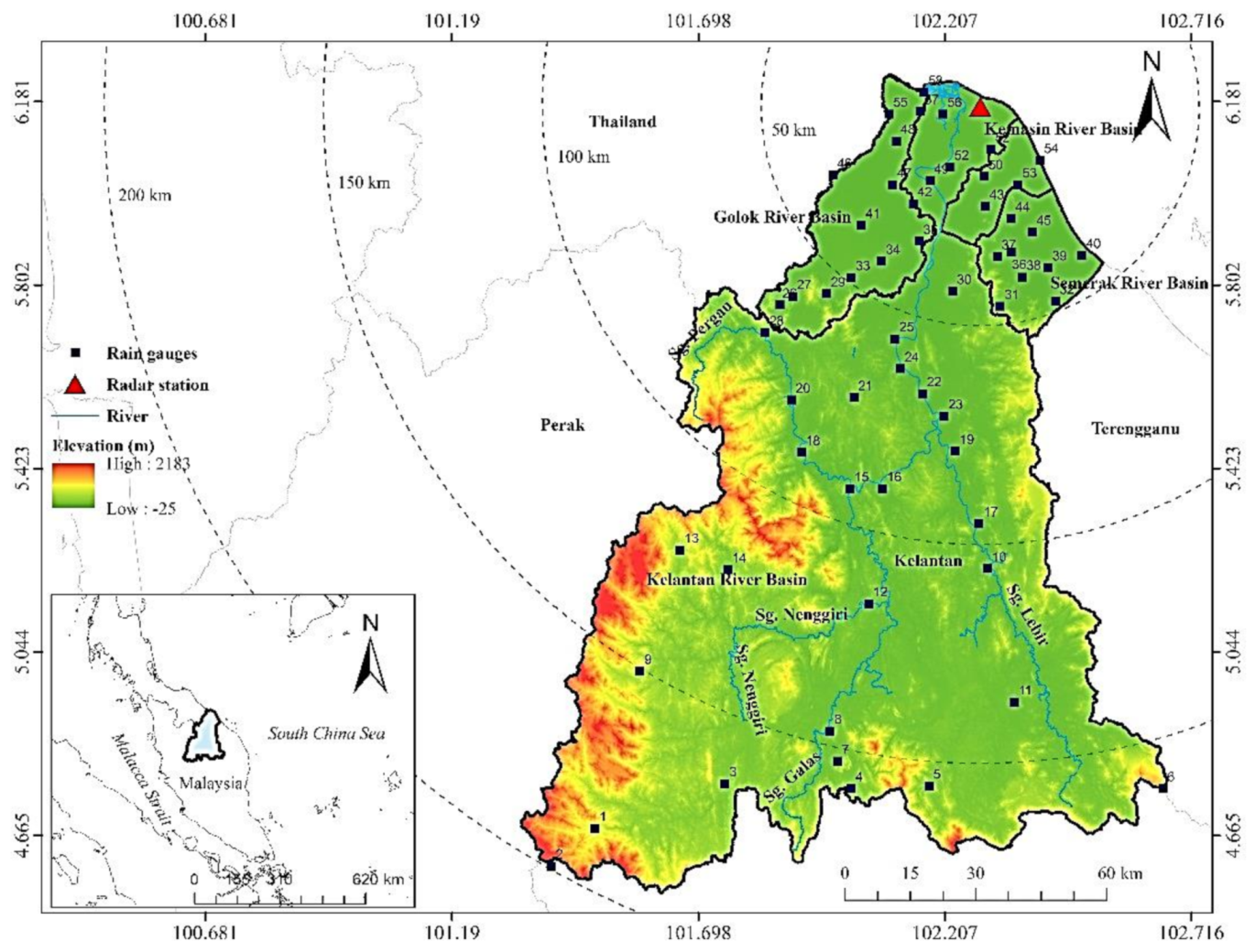
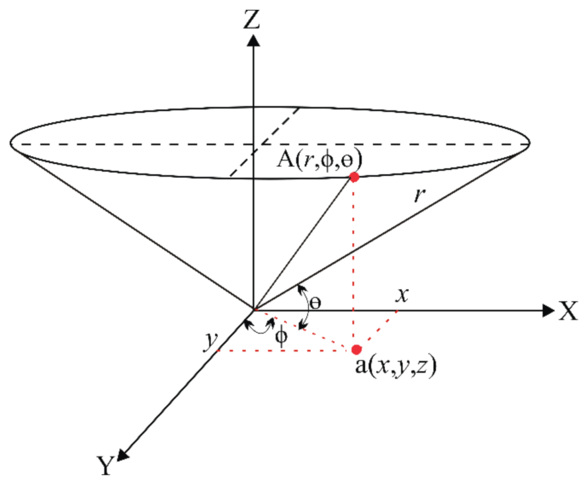
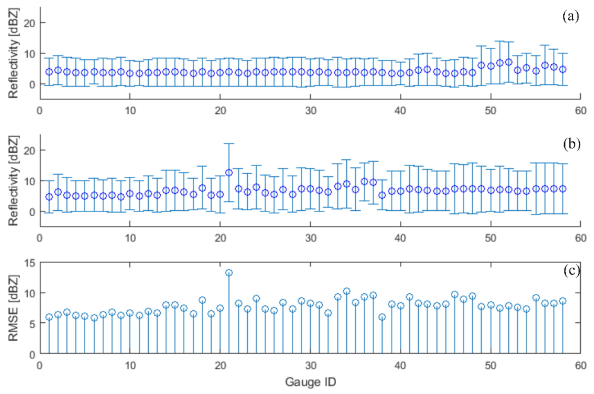
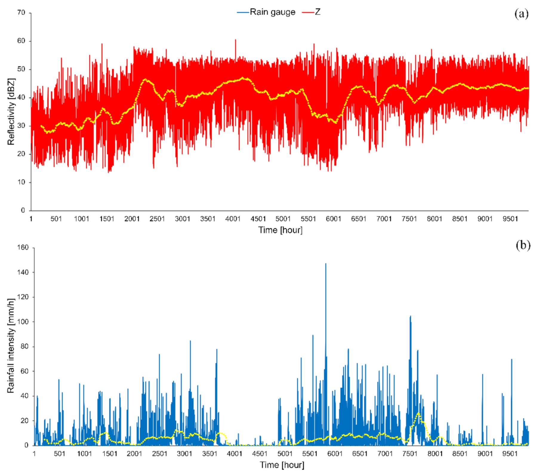
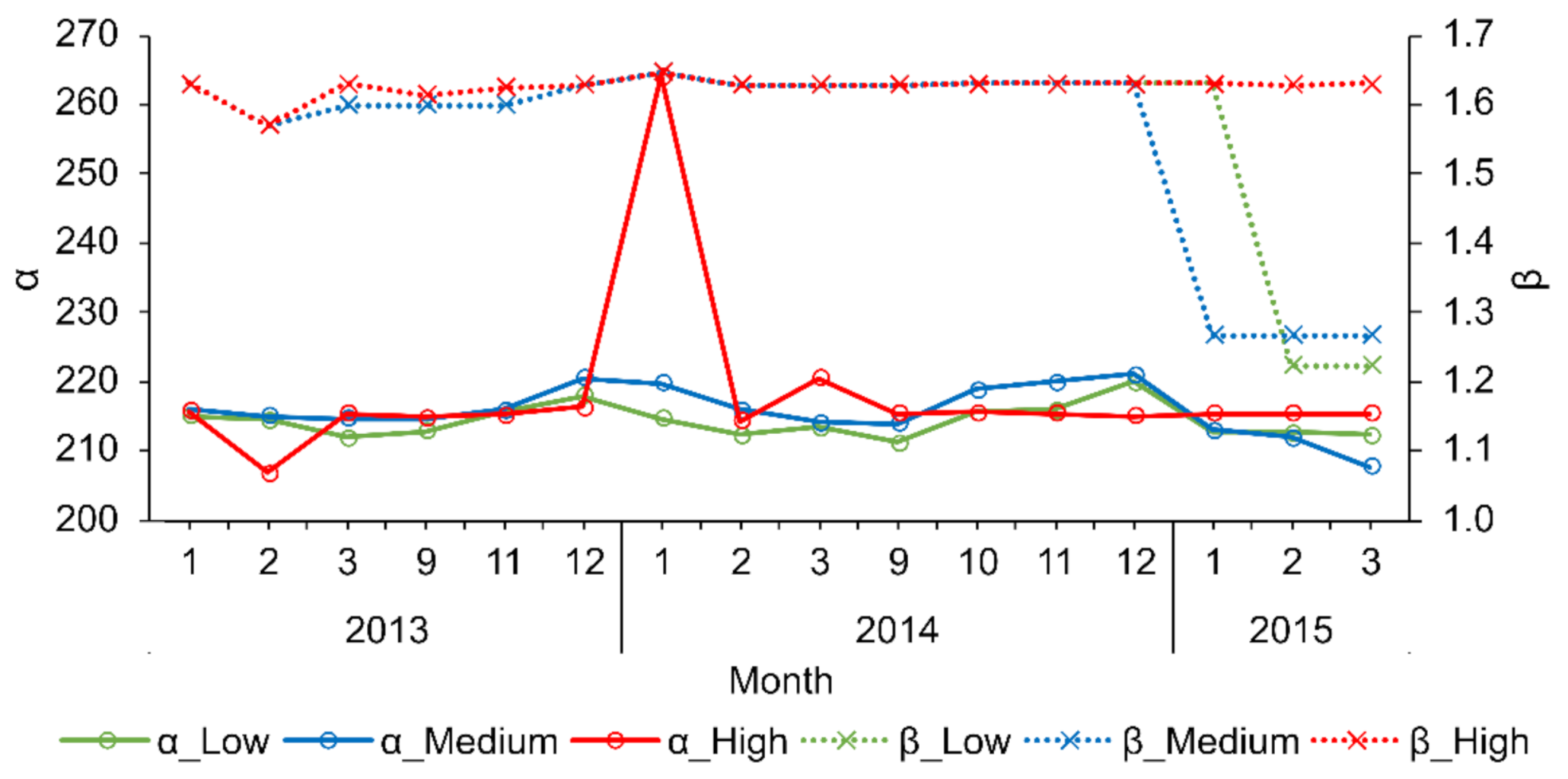
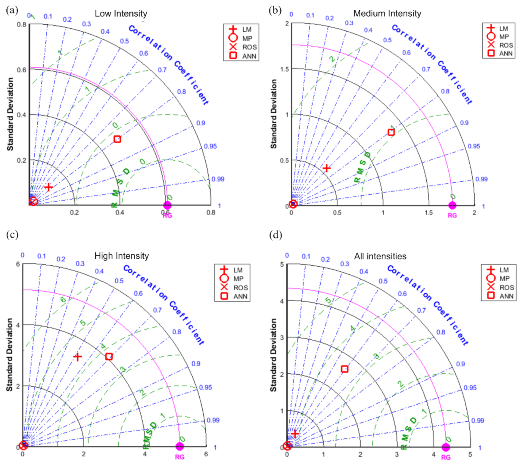
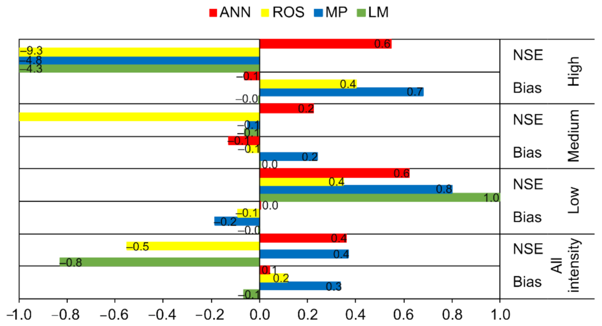
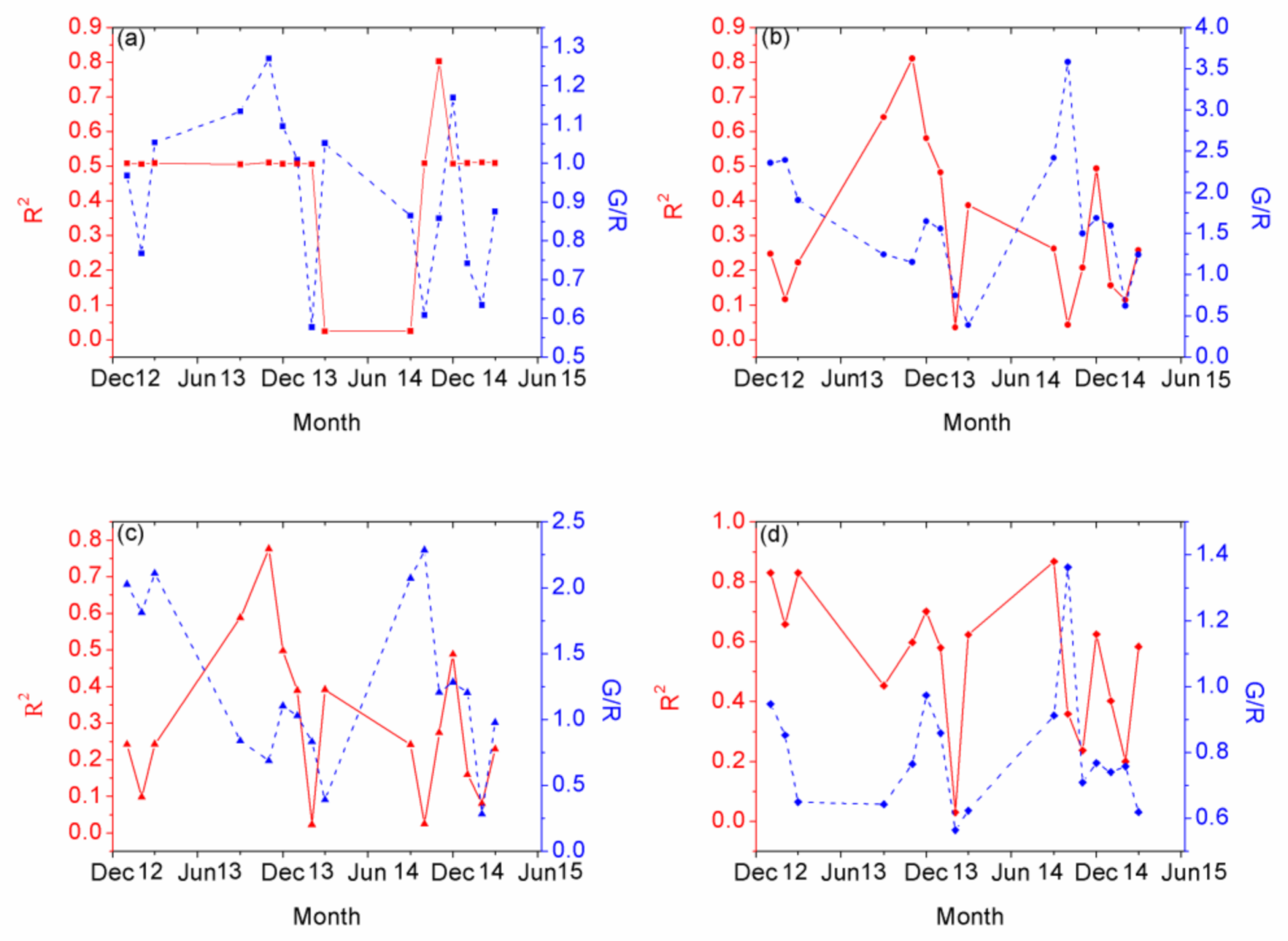
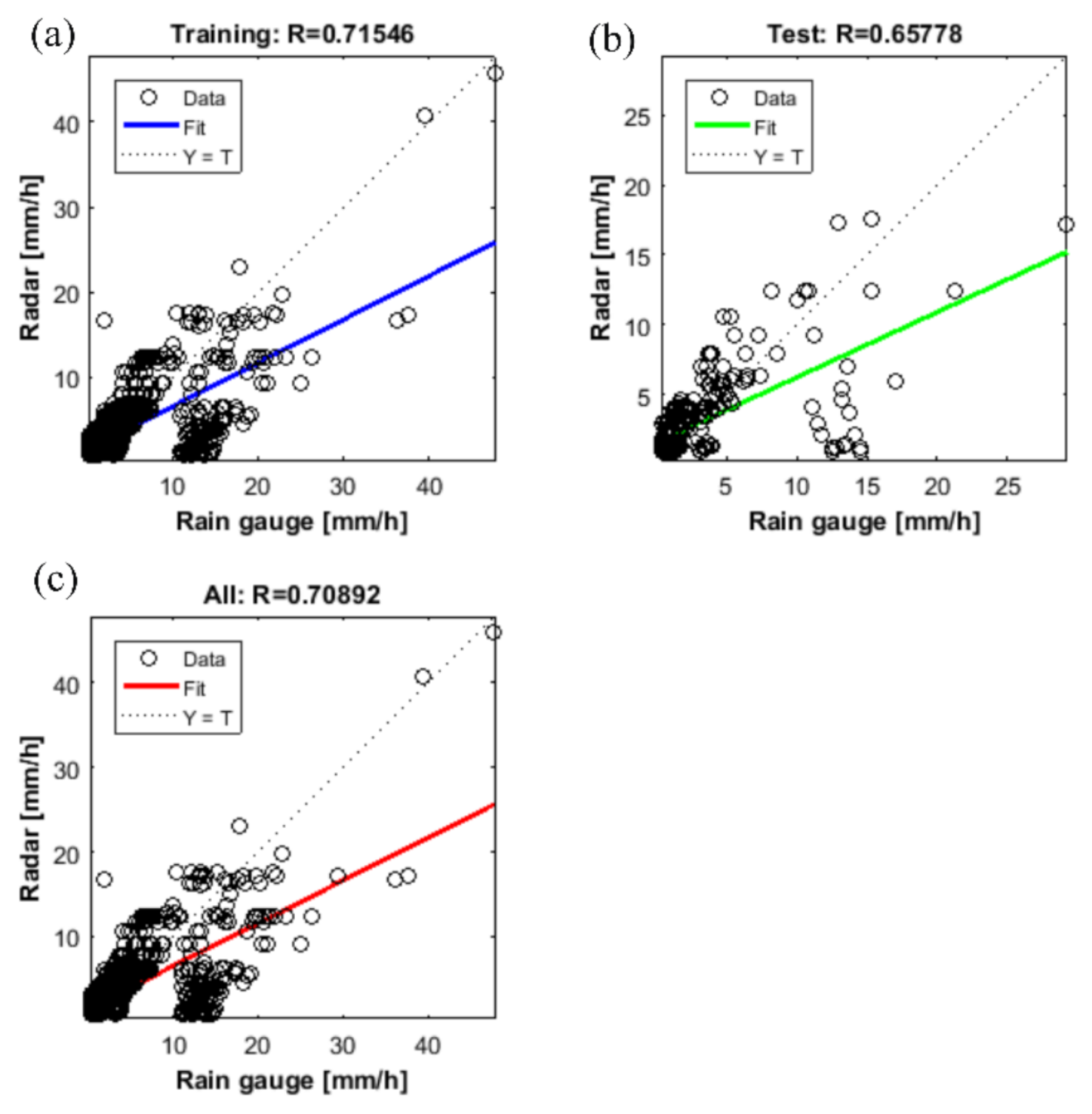
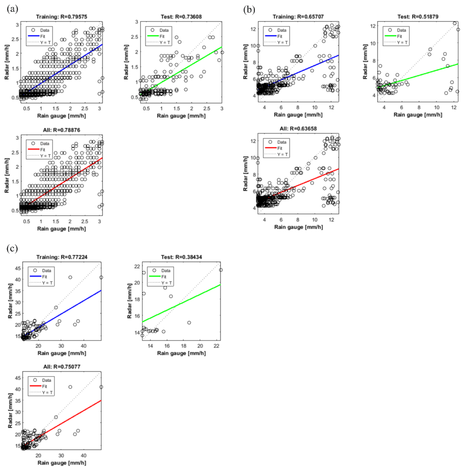
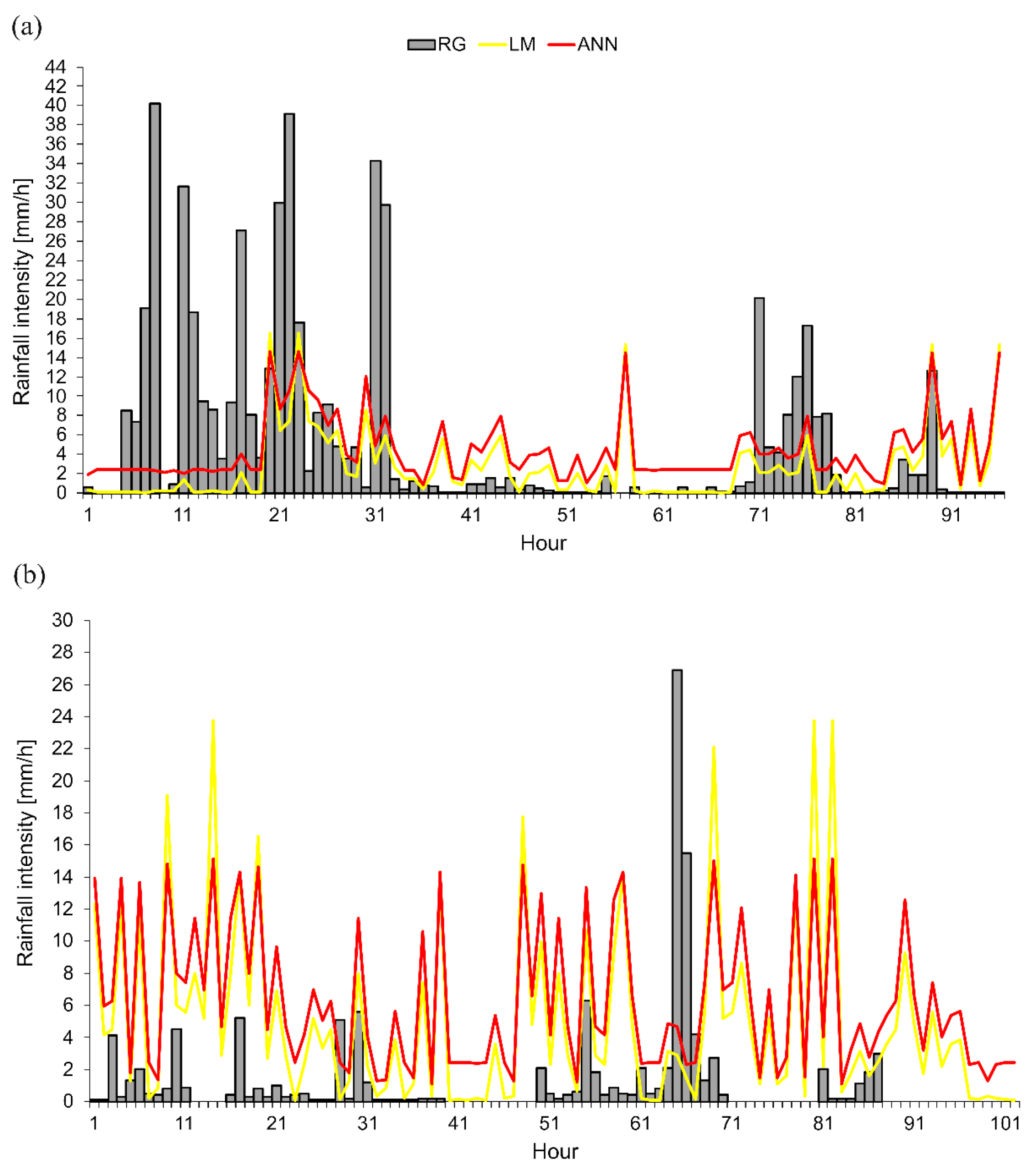
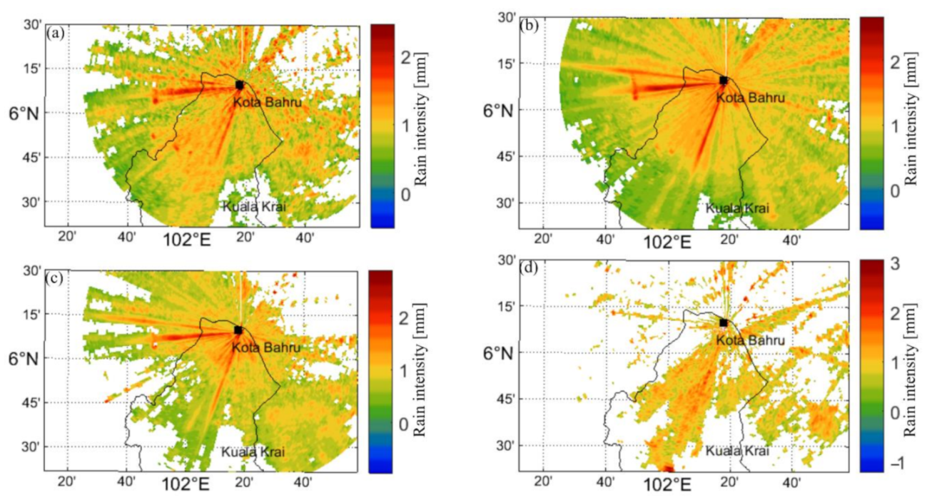
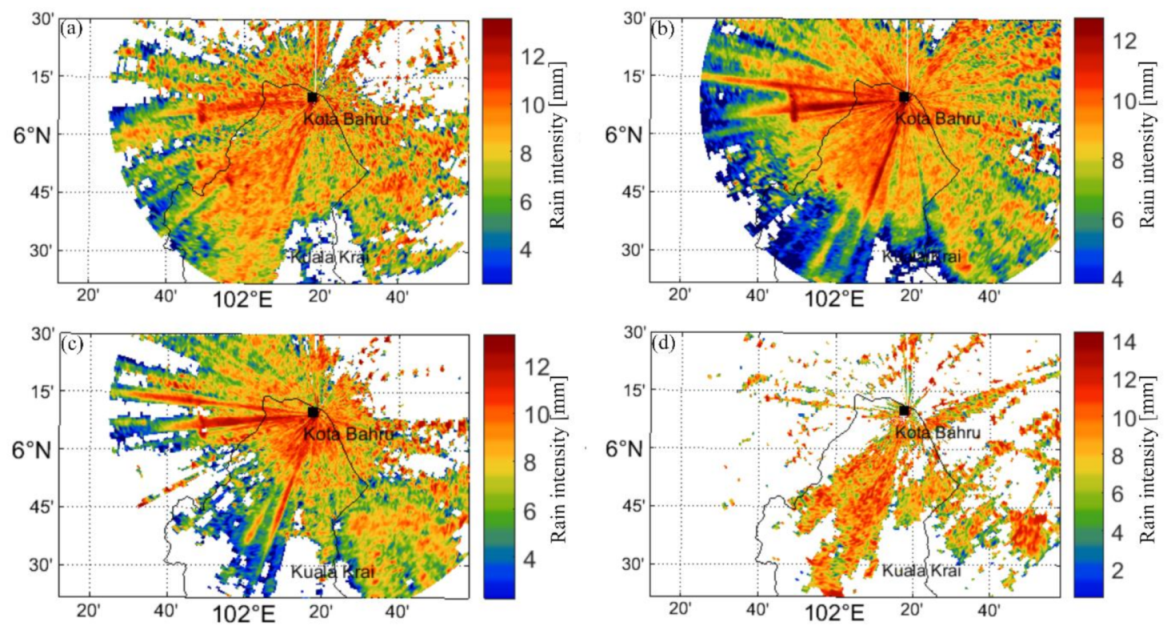
Table 1.
Technical specification for Kota Bahru (KB) weather radar.
| Specification | Description |
|---|---|
| Model | EEC WSR 745/1996 |
| Peak power | 500 kW |
| Pulse width | 2.0 µs |
| Gain | Minimum 39 dB |
| Pulse response frequency | 250 Hz |
| Beamwidth | 1.9 degree maximum on axes |
| Elevation range | 0.0, 0.7, 1.5 and 2.5 degree |
| Threshold LOG | 0.75 dB |
| Threshold CSR | 18 dB |
Table 2.
α and β coefficients of newly established Z-R models for different rain intensities.
| Intensity Type | Optimized Z-R |
|---|---|
| All intensity | Z = 216.3 R1.6 |
| Low | Z = 214.3 R1.6 |
| Medium | Z = 215.9 R1.6 |
| High | Z = 218.2 R1.6 |
Publisher’s Note: MDPI stays neutral with regard to jurisdictional claims in published maps and institutional affiliations. |
© 2021 by the authors. Licensee MDPI, Basel, Switzerland. This article is an open access article distributed under the terms and conditions of the Creative Commons Attribution (CC BY) license (https://creativecommons.org/licenses/by/4.0/).
Share and Cite
MDPI and ACS Style
Roslan, N.; Md Reba, M.N.; Sharoni, S.M.H.; Hossain, M.S. The 3D Neural Network for Improving Radar-Rainfall Estimation in Monsoon Climate. Atmosphere 2021, 12, 634. https://0-doi-org.brum.beds.ac.uk/10.3390/atmos12050634
AMA Style
Roslan N, Md Reba MN, Sharoni SMH, Hossain MS. The 3D Neural Network for Improving Radar-Rainfall Estimation in Monsoon Climate. Atmosphere. 2021; 12(5):634. https://0-doi-org.brum.beds.ac.uk/10.3390/atmos12050634
Chicago/Turabian StyleRoslan, Nurulhani, Mohd Nadzri Md Reba, Syarawi M. H. Sharoni, and Mohammad Shawkat Hossain. 2021. "The 3D Neural Network for Improving Radar-Rainfall Estimation in Monsoon Climate" Atmosphere 12, no. 5: 634. https://0-doi-org.brum.beds.ac.uk/10.3390/atmos12050634
Note that from the first issue of 2016, this journal uses article numbers instead of page numbers. See further details here.