
Impact of Industrial Air Pollution on Agricultural Production


1
Key Research Institute of Yellow River Civilization and Sustainable Development, Henan University, Kaifeng 475000, China
2
School of Business and Tourism Management, Yunnan University, Kunming 650000, China
*
Author to whom correspondence should be addressed.
Atmosphere 2021, 12(5), 639; https://0-doi-org.brum.beds.ac.uk/10.3390/atmos12050639
Submission received: 11 April 2021
/
Revised: 10 May 2021
/
Accepted: 13 May 2021
/
Published: 18 May 2021
(This article belongs to the Special Issue Air Quality and Climate Effects of Traditional and Emerging Pollutants)
Abstract
:This paper aimed to study how industrial air pollution impacts crop yield by investigating the relationship between output and changes in factors. A translog production function was estimated in the context of stochastic frontier analysis using data collected from a field survey in the case of corn. The interaction between the factors as well as the impact of industrial air pollution on the relationship between factors was analyzed using numerical simulation, followed by the estimation of economic losses of corn yield in the polluted area. Results show that industrial air pollution causes a decrease in crop yield for two reasons. First, industrial air pollution changes the output elasticities of production factors and reduces its absolute amount. Second, industrial air pollution causes the relationship between labor and capital, labor and chemicals, capital and seeds to change from substitutable to complementary; it also resulted in an opposite result for the relationship between capital and chemicals. The paper presents a new explanation of how industrial air pollution affects agricultural production from an economic perspective.
1. Introduction
Industrial air pollution not only affects human health, but also has a negative impact on agricultural activities, resulting in huge welfare losses. The direct economic loss on agricultural production and the indirect harm on other receptors is a worldwide political and scientific issues [1] Assessing the external costs not only provides information to assess the economic feasibility of polluting industrial activities but can also serve as input for policy making.
There are four main sources of air pollutants based on the industrial activity [2]: (1) carbon monoxide, oxides of sulfur, oxides of nitrogen and dust from the combustion process; (2) photochemical oxidants, carbon monoxide and sulfuric acid fumes from the stationary processes, including furnaces, refineries, etc.; (3) toxic organic gases from the process of hazardous wastes; (4) hydrocarbons, oxides of nitrogen, carbon monoxide and particulate from the mobile process, which can be defined as one capable of moving from one place to another under its own power.
Air pollution affects agricultural productivity in two ways [3]: (1) pollutants disrupt plants’ biochemical and physiological reactions to a certain degree, and (2) acid rain resulting from air pollution causes soil degradation and lowers the concentration of nutrients that crops need. These effects are cumulative and permanent.
Many studies show that industrial air pollution has a significant impact on crop growth and yield. Crop yield depends largely on ambient conditions, especially air quality. Air pollution can result in a reduction in crop yield. For example, in the United States, economic losses due to air pollution were USD 40–50 billion in 1997 [4]; in Pakistan, when the seasonal average concentration of O3, NO2 and SO2 were 70 ppb, 28 ppb and 15 ppb, the yields of three rice varieties decreased by 43%, 39% and 18%, respectively, during the 2003–2004 season [5].
There are four methods usually used to assess agricultural losses from industrial air pollution. The first one is the dose-response equation, which is established using field experimental data to show the relation between the actual or estimated losses and the concentration of pollutants [6,7]. The second one is the field comparison test. For example, Rai and Agrawal [8] used the open-top chamber method to study wheat and rice yields’ change after being affected by a certain degree of SO2, NO2 and O3. The third one is the method of regional comparison, which analyzes the impact of industrial air pollution on crop yield by selecting two regions with the same natural conditions and social characteristics. One area is contaminated while the other area is not affected by industrial air pollution [9,10]. The fourth one is estimation using existing models. Humblot et al. [11] combined a biophysical crop model with an economic supply model to predict and quantify the effect of industrial air pollution on agriculture. The biophysical crop model provides a yield function based on environmental conditions and fertilizer inputs, while the economic model is a mathematical programming model.
However, most of the existing literature use experimental data and dose-response equation to estimate economic losses due to air pollution. This method still has some problems because of the lack of a generalized dose-response function. The existing methods on the relationship among pollutants, crop yields and quality are not consistent. The existing dose-response function was constructed using data from a specific area and a specific mix of pollutants and may not reflect the real situation as it is used elsewhere [7]. There appears to be a lack of a systematic study on the effects of air pollutants on crop yield, which are affected by the emission patterns of pollutants, atmospheric flow and amount of pollutants that the crop leaves absorb, as well as the biochemical resistance of crops to pollutants [8].
In some developing countries, pollution monitoring stations, equipment, funds and related human resources are limited, making it difficult to assess the impact of industrial pollution on agriculture by conducting experiments or constructing dose-response functions [12]. Moreover, because large databases and industrial economic model on agricultural production are lacking, it is also difficult to estimate the impact of pollution on agriculture based on existing models. In particular, agricultural loss is associated with producers’ change in their inputs and production behaviors [13], but the above-mentioned methods cannot address these issues.
There are a few papers that used producers’ input and output data (for example [9]), as well as socio-economic data to assess the agricultural losses resulting from air pollution. However, there is still lack of study on how air pollution affects the production function of crop yield, in which the marginal outputs of factors and the relationships between factors may be altered. This paper aims to fill this gap by studying the impacts of industrial air pollution on agricultural output.
The paper aims to estimate the external cost of industrial air pollution on agriculture by exploring the ways of industrial air pollution affecting factor’s marginal output and the relationship between factors. The studied crop is corn. The study site is a silicon industrial park and its surrounding area in southwest China. The silicon industrial park was set up in 2008, and it has eight silicon plants so far, whose main product is metallurgical silicon. Due to the rapid development of the world photovoltaic industry in recent years, the park’s output also grew rapidly. The output was 5000 tons in 2008 and increased to 8.5 million tons in 2014. The main air pollutants of industrial silicon production are SO2, NOx, CO and PM [14]. In order to reduce production costs, silicon plants do not install abatement equipment or do not use it even if installed. As a result, silicon production activities cause serious air pollution on local environmental receptors.
The paper is composed of five parts. The first part is an introduction of research background and problems. The second part presents theoretical hypotheses and research methods. The third part discusses data sources and statistical analysis. The fourth part presents the empirical results and its explanation. The last part is conclusions and policy implications.
2. Theoretical Hypothesis and Research Method
2.1. Theoretical Hypothesis
Unlike the existing literature that directly compare the economic values of polluted and non-polluted crops, this study tries to explore how industrial air pollution reduces crop yield by affecting the relationship between production factors based on the production function theory. From this point of view, the following hypotheses are formulated:
Hypothesis 1.
The relationship between agricultural yield and inputs of factors is to be altered by industrial air pollution.
Crop yield is usually affected by its ambient conditions, especially air quality. Studies revealed that industrial air pollution can greatly lower crop yield [4,5,7,10]. According to Aragon and Rud [15], air pollution can reduce crop yield by 30–60%, in terms of different crop and pollutants. Many dose-response functions have established the relationship between yield loss and pollutant concentration [7,8,9].
Since air pollution can more or less disrupt the crops’ biochemical and physiological reactions [3], the productivities of factors such as nutrients and labors are also expected to be changed. Furthermore, industrial air pollution has different interactions with different factors [9,16].
Based on the evidence that industrial air pollution affects both the yield and the factors’ productivities, it can be inferred that industrial air pollution can alter the production relationship between crop yield and inputs of factors.
Hypothesis 1 (H1A).
Industrial air pollution changes the relationship between a factor and its output elasticity.
As an effect of industrial air pollution, a reduction in crops’ yield and factors’ productivities implies that the output elasticity of factor is changed. Neeliah and Shankar [17] estimated the production functions of cereals in England using a panel dataset, which showed that there is a significantly negative relationship between total output elasticity and tropospheric ozone concentration.
There are two reasons why industrial air pollution reduces the output elasticity of production factors. First, pollutants alter crops’ biochemical and physiological reaction to a certain degree [3], making crops less effective in absorbing nutrients. Second, industrial air pollution results in soil degradation and eventually reduces the carrying capacity of farmland.
Hypothesis 1 (H1B).
Industrial air pollution can alter the substitution or complementary elasticity between production factors.
There is no available study of the effect of industrial air pollution on substitution elasticity, but many scholars analyze that technological progress affects the substitution elasticity. For example, Blankenau and Cassou [18] explored that technological progress can alter the substitution elasticity between different types of labor; Lin and Fei [19] found that three factors are substitutes for one another in agricultural sector. Industrial air pollution has a role like technological progress in agricultural production, but its effects are negative.
Like many other production activities, agricultural production requires inputs of man factors, including nutrients, labor and capitals. Industrial air pollution can alter the set of production factors in terms of the ratio of inputs and the quantity of each factor. Moreover, producers may have different behavior in choosing inputs in the presence of industrial air pollution. In particular, industrial air pollution has different interactions with different factors [9,16].
Thus, the factors’ substitution or complementary elasticity can be changed by industrial air pollution.
2.2. Research Method
The assessment of the impacts of industrial air pollution on agricultural production was carried out as follows. First, two regions with similar natural and socio-economic characteristics were selected for data collection; one is the polluted area while the other is the non-polluted area. Data sets from the two areas were classified as the polluted group and the reference group. Second, three translog production functions were estimated based on Stata, two using each dataset and one using the pooled data. Based on the three production functions, the impacts of industrial air pollution on agricultural production were analyzed and Hypothesis 1 was tested. Third, using R software package [20,21,22,23], Hypothesis 1A was tested by comparing the output elasticity of production factors in the polluted group and the reference group. Fourth, Hypothesis 1B was tested by comparing the elasticities of substitution and complementary of production factors in the two data sets. Final, the economic losses of agricultural production resulting from industrial air pollution was estimated, using the estimated models and considering three scenarios.
2.2.1. Model
This study used the translog production function instead of the Cobb-Douglas production function [24] because of the former’s flexibility in analyzing the relationships between different variables in the production function. That is, the relationship can be analyzed by including the quadratic form of factors and the interaction between factors [25]. The translog function is expressed as follows:
where represents the logarithm of output; represents the logarithm of the ith input; is the interaction between factors; , and are the coefficients to be estimated; D is the variable representing the level of industrial air pollution; is the interaction between production factor and industrial pollution; represents the socio-economic characteristics of respondents and their households, including gender and years of schooling; n and k are the numbers of factors and socio-economic variables; and is the error term.
Production factors are labor (L), capital (K), seeds (S) and chemicals (C, including fertilizers, pesticides and herbicides). The variable of industrial pollution, D, is represented by the proxy of the straight distance from the farmland to source of industrial air pollution. As the concentration of pollutant tends to decrease as the distance from the pollution source becomes farther, the distance is a reasonable proxy for the level of industrial air pollution that crops receive. The agricultural output is also affected by the socio-economic characteristics (Z) of producers, including respondents’ gender (Z1), educational attainment (Z2) and number of family members (Z3). The translog model to be estimated was expressed as:
where is the observation.
The restriction of Equation (3) was used to test the existence of a Cobb-Douglas production function. That is, the production function is in the form of CD if Equation (3) is satisfied.
2.2.2. Relationship between Production Factors
In a production function, it is possible for the relationship between two factors to be substitute or complementary. The relationship can be estimated using the following equation [22]:
where and represents the ith and the jth production factors; and are the marginal output of the ith and the jth factors.
Two factors are substitutable , and complementary . In addition to its direct impact on agricultural output, industrial pollution also has an indirect impact on agricultural production by indirectly affecting the relationship between factors. Thus, the impact of industrial air pollution on the relationship between factors can be reflected from the changes in .
The production function is usually estimated using the ordinary least squares method (OLS), whose basic assumption is that the producer maximizes profit or minimizes production cost at a certain output level. However, it is usually impossible to meet this requirement for ordinary producers in the actual production activities [26]. Thus, the study uses the stochastic frontier analysis (SFA) method, instead of using the OLS to estimate production functions.
2.2.3. Estimation of Economic Losses
Whether it affects agricultural production via industrial air pollution will reduce crop yields or reduce the quality of agricultural products [27]. The former can be measured by changes in crop yields, while the latter can be reflected through crop market prices. Therefore, the economic losses (EL) of a certain crop can be estimated by using the following formula:
where P represents the market price of quality product; and are the average crop outputs in non-polluted area and polluted area, respectively; is the price difference between quality and low-quality products.
In order to identify the economic loss from industrial air pollution, the quantification of output loss is essential. Agricultural output is affected by many factors, including cultivation practices and the socio-economic characteristics of farmer household. The difference in output is thus to be quantified based on the same set of inputs. Except for the variable of industrial air pollution, the value of all other inputs for the agricultural production should be the same. We also set three scenarios, all other inputs take their own minimum value, respectively, called as the “Min” scenario. Similarly, another two scenarios are the “Mean” and “Max” scenario. Thus, the difference of output can be estimated using the estimated production function for the reference group and the polluted group, as shown in Table 3.
3. Data and Descriptive Statistical Analysis
3.1. Data
The study area is Nujiang prefecture, which is located in southwest Yunnan province, China. Despite its abundance in natural resources, this prefecture is underdeveloped with few industries.
To promote the regional economic development, the Nujiang government takes great effort in introducing investment to explore its natural resources. A silicon industrial park was built in 2006 and completed in 2008 to introduce investors to produce metallurgical silicon. In the past several decades, Nujiang, as a primitive area, was free of environmental pollution because of few industrial production activities. As silicon industries were introduced to this prefecture, environmental quality has been greatly reduced.
The production of metallurgical silicon is the initial section of the industrial chain of solar energy generation, in which SiO2 in sand or quartzite is reduced to Si in an arc furnace. The main air pollutants of industrial silicon production are SO2, NOx, CO and PM [14]. In order to reduce the production costs, silicon plants do not install abatement equipment or do not use them even if installed. As a result, silicon production activities caused serious air pollution.
To assess the impact of pollution on crops, the study selected two villages A and B for comparison. Village A is the area where the silicon industrial park is located and is thus severely affected by industrial air pollution. Data from this village was viewed as the data of polluted group. Located about 30 km from the silicon industrial park, village B is free of industrial air pollution and thus data from this village was used as the reference. Both villages have similar natural environment characteristics, such as vegetation, climate and soil type, and high similarity in social characteristics like agricultural practices and ethnic and lifestyle aspects. There are two major differences between the two villages. First, the distance from the different pollution sources is different.
All the data was collected through face-to-face interviews. The questionnaire design was based on literature research and the results of focus group discussions, including socio-economic conditions of farmers and information of agricultural production activities. In order to enhance its appropriateness and effectiveness, the questionnaire was revised through a pilot survey.
Villages A and B have 1016 farmers and 806 farmers, respectively. Given the financial constraints, the sampling error was set to 7.5% and the two villages’ samples were set at 151 and 145, respectively. Assuming an invalid questionnaire rate of 20%, the sample sizes for survey in the two villages were 180 and 175, respectively. Responding households were randomly selected in each village. The surveys were completed between December 2014 and February 2015. Eventually, a total of 333 copies of valid questionnaires were collected, including 158 for the polluted group and 165 for the reference group.
3.2. Descriptive Statistical Analysis
The descriptive statistical analysis of the data is shown in Table 1. As mentioned above, village B is 30 km from the silicon industrial park, while the average distance of surveyed households to the silicon industrial park is 3.67 km. There were more male respondents than female respondents in the polluted group, while the numbers of male and female respondents were nearly equal in the reference group. There was no obvious difference in the level of education, number of family members and per capita household income among the interviewees. As a whole, the average acreage of farmland in the polluted group was a little higher, while the yield per acre was slightly lower than in the reference group. As far as inputs were concerned, the inputs of labor, capital, fertilizers and pesticides per unit of farmland in the reference group were slightly higher than in the polluted group. However, the input of seed per unit of farmland in the polluted group was higher than in the reference group. In addition, there are 80 males and 85 females in the reference group, and the polluted group includes 122 males and 46 females. This study sets Z1 as a dummy variable with “Male (M) = 1” and “Female (F) = 0”, so we may compute the mean and standard deviation for the two groups.
The reason for higher seed inputs in the polluted group may be that industrial air pollution has resulted in a lower rate of seed germination. Due to the lower unit yield, labor and capital inputs for harvesting were correspondingly lower in the polluted group. In addition, as the growth of seeds is limited by industrial air pollution, more unit input of fertilizer was required in the polluted group.
4. Empirical Results and Explanation
4.1. Translog Production Function of Corn
The estimated results of the translog production function are shown in Table 2. Three models were estimated. Model I was estimated from the pooled data, model II from the reference group data and model III from the polluted group data. To achieve unbiased estimation, the robustness was checked. First, the multicollinearity between explanatory variables was checked according to the correlation matrix. The correlation between the explanatory variables is less than 20%, i.e., the correlation is very weak. Second, the homoscedasticity was tested using the White test method [28]. The chi2 statistics are 201.61 (p = 0.3207), 136.63 (p = 0.1285) and 122.00 (p = 0.4574) for the three models, respectively and all of them do not reject the null hypothesis of homoskedasticity. Third, the presence of excessive variables in the production function was checked using the Wald chi-square value. As calculated, the Wald chi-square value of the three production functions were 1837.32, 586.73 and 3482.30, respectively, and their p values are 0.0000. These show that there are no excessive variables in the estimated production functions.
The results of model I show that most input factors like labor and the interaction coefficients are statistically significant, and that the coefficients of the industrial air pollution variable and its interaction with other factors are also statistically significant. The coefficient of the variable of family members is significant at the 95% confidence level.
On the other hand, model II shows that the coefficients of most factor variables and the interaction are significant. However, the impact of an increase in a factor input (say, labor) on the output is uncertain because the result was jointly decided by labor, capital input, seed inputs and chemical inputs. The coefficient of gender is significant at 90% confidence level. If farmers were men, corn output will increase 0.042% than in the case of female farmers.
In model III, the interactions of factors are statistically significant. However, the significant level is slightly lower than the corresponding results in model II. As in model II, the impact of a change in a single factor input on output is determined by all other factors. The coefficients of number of family members is significant at 95% confidence level. More importantly, the coefficients of the intersections between the industrial air pollution variable and factors are significant, which can provide a good base for the following analysis.
Compared with the conditions of the constant return to scale, the sums of the coefficients of factor variables, , are −2.202, −2.962 and 3.685 for the models I, II and III, respectively. That is, the estimated production functions do not have the characteristics of constant return to scale. The coefficients of the quadratic terms and the interaction terms are also significant. Since the restriction of Equation (3) is not satisfied, the estimated translog production function cannot be simplified to a Cobb-Douglas production function. With non-constant elasticity of substitution between factors, the translog production function was found to be more suitable to describe the relationship between output and factors than the Cobb-Douglas production function whose elasticity of substitution is constant. Therefore, Hypothesis 1 is proved.
4.2. Impact of Industrial Air Pollution on Agricultural Output
Intuitively, the stronger industrial air pollution is, the greater the agricultural loss will be. There are three reasons for this relationship. First, the closer distance from the industrial air pollution to cornfield is, the higher the concentration of pollutants and thus the greater inhibition on the growth of crops. Second, a more severe industrial air pollution is more likely to reduce the output elasticity of production factor, and thus indirectly affects the output of crops. Third, industrial air pollution also changes the substitution relationship between factors, reflected by the substitution elasticity and indirectly affects the output. From this point of view, the study analyzed the impact of industrial air pollution on the output of corn by taking all production factors, industrial air pollution and their interaction into consideration.
The coefficient of D and its square term can reflect the direct impact of industrial air pollution on corn output. It should be noted that in Model I and Model III, the coefficients of the square term of D are both significant at the 99% confidence level, but the signs are opposite. Among them, the coefficient of Model I is counterintuitive, because the reference group assumes that all observations of D are the same, and the relationship between the corn yield and distance is irrelevant. Once the two groups of data are mixed together, this can distort the above relationship. Therefore, when studying the direct impact of industrial air pollution on corn output, the coefficient of D in Model III and its square term is more meaningful.
According to the coefficient of D and its square term in Model III, the critical point is −2.938 km (less than zero), which means that as the distance from the observation point to the point pollution source increases, the corn yield will increase with the same inputs. Distance is a proxy for the concentration of industrial air pollution. The greater the distance, the lower the concentration is. In sum, the negative impact of industrial air pollution on corn yield is significant, and the impact increases as the pollutant concentration becomes higher.
Next, we will explain why industrial air pollution causes a decline in corn production from two aspects of output elasticity and substitution elasticity.
4.3. Impact of Industrial Air Pollution on the Output Elasticity of Production Factors
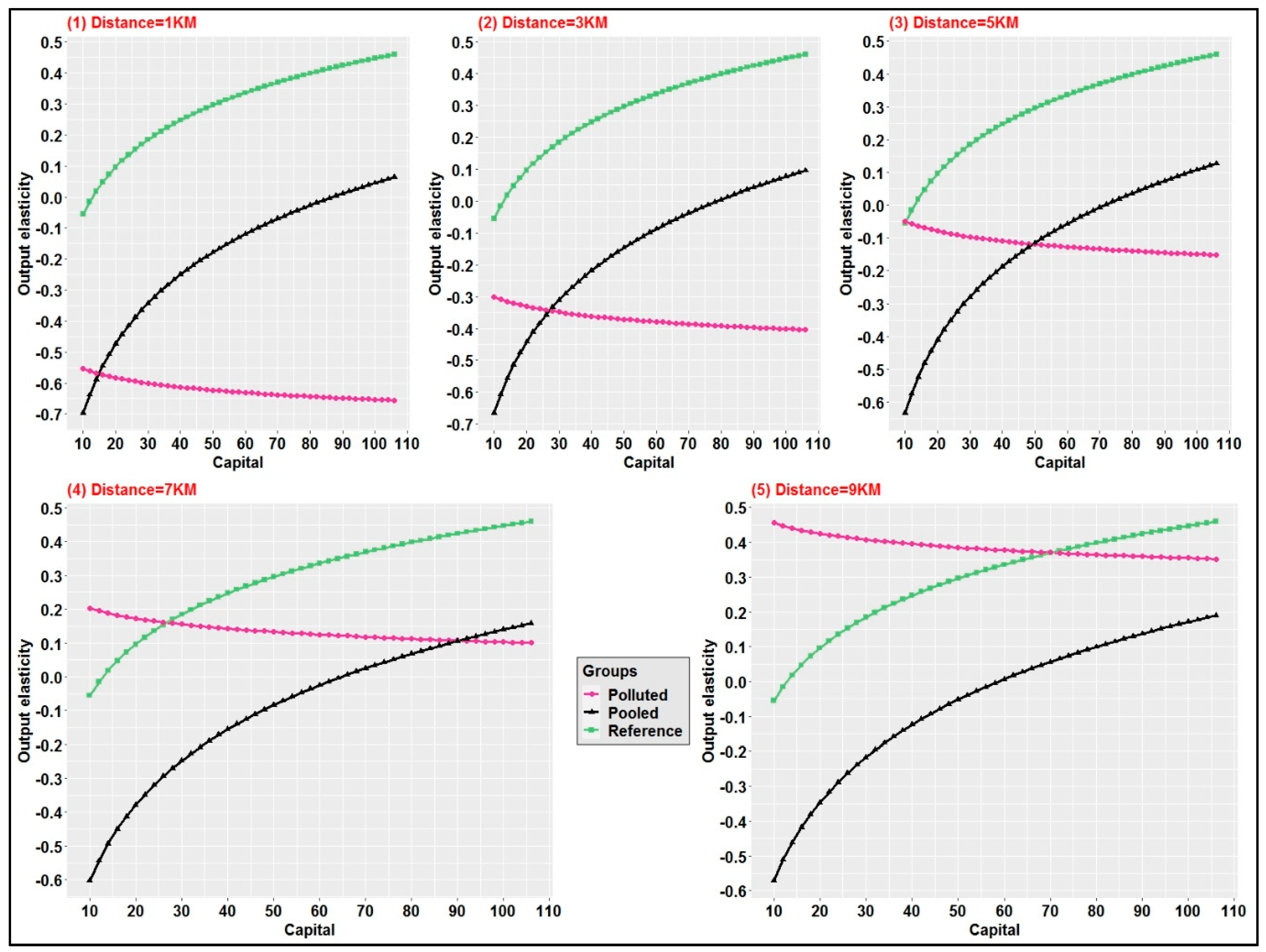
This section analyzes the impact of industrial air pollution on the input factors and the indirect effects on output in greater detail. Taking capital as an example, the impact of industrial air pollution on the output elasticity of factors is analyzed using the numerical simulation method.
As shown by the coefficients of the interaction terms in Table 2, a change in industrial air pollution has an indirect effect on capital input. Thus, it is difficult to quantify the impact of a change in a factor on the output. Instead, the impact was analyzed by simulation. That is, holding the input of other factors constant, we simulate how the output elasticity of capital changes as D (Distance) changes. In addition, the reference group is used as the references here.
As shown in Figure 1, the main difference between the five subfigures is the D variable’s value. In each subfigure, the output elasticity of capital for three groups is simulated, respectively, including the reference group, the polluted group and the pooled group. First, while fixing the D’s value. With the increase of capital input, the output elasticity in the reference group is positive and gradually increases, but the output elasticity in the polluted group corresponds to an opposite result. This implies that industrial air pollution has changed the relationship between capital and its own output elasticity, that is, the relationship has changed from a positive correlation to a negative correlation. For example, industrial air pollution has led to a reduction in corn production. Even if farmers increase their capital investment in farming, the output will increase slightly, but it is far smaller than the increase in capital input. Overall, the output elasticity of capital can decrease as capital input increases.
Furthermore, there is an exciting finding by comparing the five subfigures comprehensively: as the concentration of industrial air pollution decreases (the D’s value becomes larger), the output elasticity in the polluted group shifts upward as a whole. This means that changes in the concentration can change the absolute amount of the output elasticity of a factor. This finding is in line with our intuition. The intensity of industrial air pollution has become weaker, and its negative impact on corn production has also been reduced. The characteristic of the output elasticity in the polluted group are more similar to that in the reference group. Furthermore, the change in the output elasticity in the pooled group is similar to that in the reference group, and the absolute amount of its value also shifts upward as D’s value changes.
In summary, industrial air pollution changes the relationship between a factor and its output elasticity, and also causes a change in the absolute amount of output elasticity. Hypothesis 1A is thus proved.
4.4. Impact of Industrial Air Pollution on the Relationship between Factors
In addition to reducing the output elasticity of factors, industrial air pollution also alters the substitution or complementary relationship between factors. To verify this proposition, Allen elasticity of substitution or complementary (Henningsen, 2014) was calculated according to Equation (4).
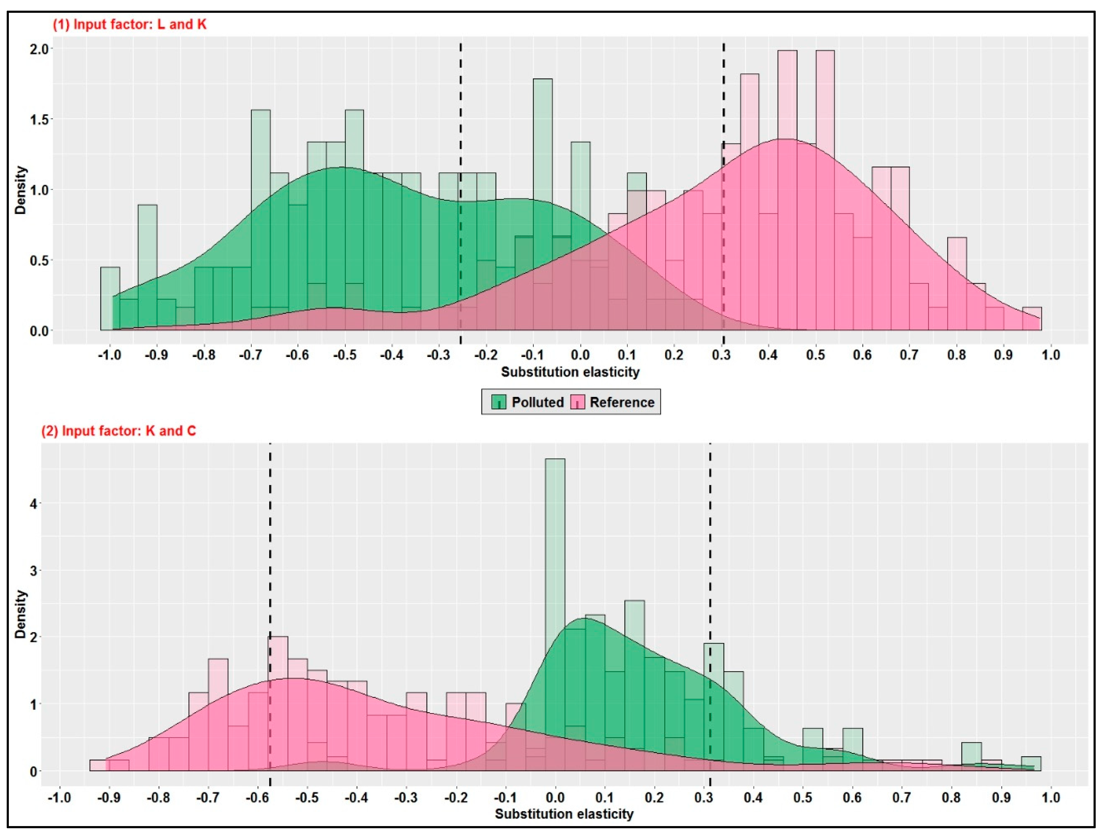
In agricultural production, the relationship between factors is not a simple substitutability or complementarity. As the production process involves different processes, there may exist substitution and complementary relationships between the two factors for the same production process. For example, compared to hand digging, using a rotary tiller can greatly reduce the amount of labor. This is the substitution relationship between labor and capital. However, the operation of a rotary tiller cannot be separated from the use of labor because the two are complementary. Similarly, compared to mechanical weeding, using herbicides can greatly reduce the use of capital, but application of the herbicide (Classified as chemicals) cannot be separated from capital. Therefore, the relationship between chemicals and capital is that they are substitutable and complementary. Due to the fact that different households have different preferences in the agricultural production process, the elasticity of substitution between factors for the same product may not be a certain value but a range of values (as shown in Figure 2).
The results show that the values of Allen elasticity of substitution of labor and seed, chemicals and seed are distributed around zero, indicating that a dominant substitution or complementary relationship does not exist between the two combinations. In the remaining four combinations, industrial air pollution changes the elasticity of factors, which can be classified into two situations: (1) the reference group is a substitution relationship, and the polluted group is a complementary relationship, including labor and capital, labor and chemicals, capital and seeds; (2) the reference group is complementary, and the polluted group is substitutional, including capital and chemicals. Therefore, we take labor and capital, capital and seeds as examples, and show the results in Figure 2.
In the first subfigure, the mean value of the elasticity of labor and capital in the reference group is around 0.4, and the histogram composed of the elasticity of all individuals is mainly located to the right of zero, and the two factors mainly show a substitution relationship; but in the polluted group, the relationship between the two is just the opposite, and the mean value of the elasticity is about −0.4. This result shows that industrial air pollution can cause some factors that are substitutable to become complementary factors. For example, when there is no industrial air pollution, farmers prefer to use manual farming alone or separately hire machinery to engage in corn production; but after industrial air pollution occurs, corn is under a pressure to reduce production and farmers intend to curb this trend. For this target, increasing the input of labor and capital (both manual and mechanical) will eventually lead to the transformation of the relationship between the two factors from the substitution to the complementary.
In the second situation, the change in the relationship between capital and chemicals is opposite to the first situation. The two factors in the reference group mainly shows a complementary relationship, while the polluted group mainly shows a substitutable relationship. Why? When corn production is not affected by industrial air pollution, farmers prefer to use herbicides and agricultural tools (classified as capital); but affected by industrial air pollution, the sensitivity of corn crops and weeds to air pollution is different and farmers may need to invest more herbicides to eradicate weeds. Considering that the total agricultural input budget remains basically unchanged, the increase in chemicals can crowd out farmers’ investment in agricultural tools and the relationship between capital and chemicals will turn into a sustainable relationship.
Therefore, industrial air pollution changes the substitution (complementary) elasticity between factors. Hypothesis 1B is thus proved.
4.5. Estimation of Economic Loss
The agricultural economic loss was estimated in three steps. First, the set of inputs was identified and quantified. Second, the outputs were estimated by inputting the values of all explanatory variables in the production functions in Table 2. Third, the economic loss was calculated by multiplying the output loss and the market price of quality corn. As surveyed, the data of corn output refers to the quantity of quality product. The quantity of low-quality corn was either small or not measured by farmers. Thus, it is impossible to estimate the economic loss of quality reduction in the study.
There are various combinations of inputs for production, and it is impossible to present all the results. As such, the study presents three basic combinations of inputs (Table 3), including the set of minimum input value, the set of mean value of input and the set of maximum input value. Since distance from farmland to the pollution source is a proxy of pollution, the shortest distance represents the maximum pollution that crops receive.
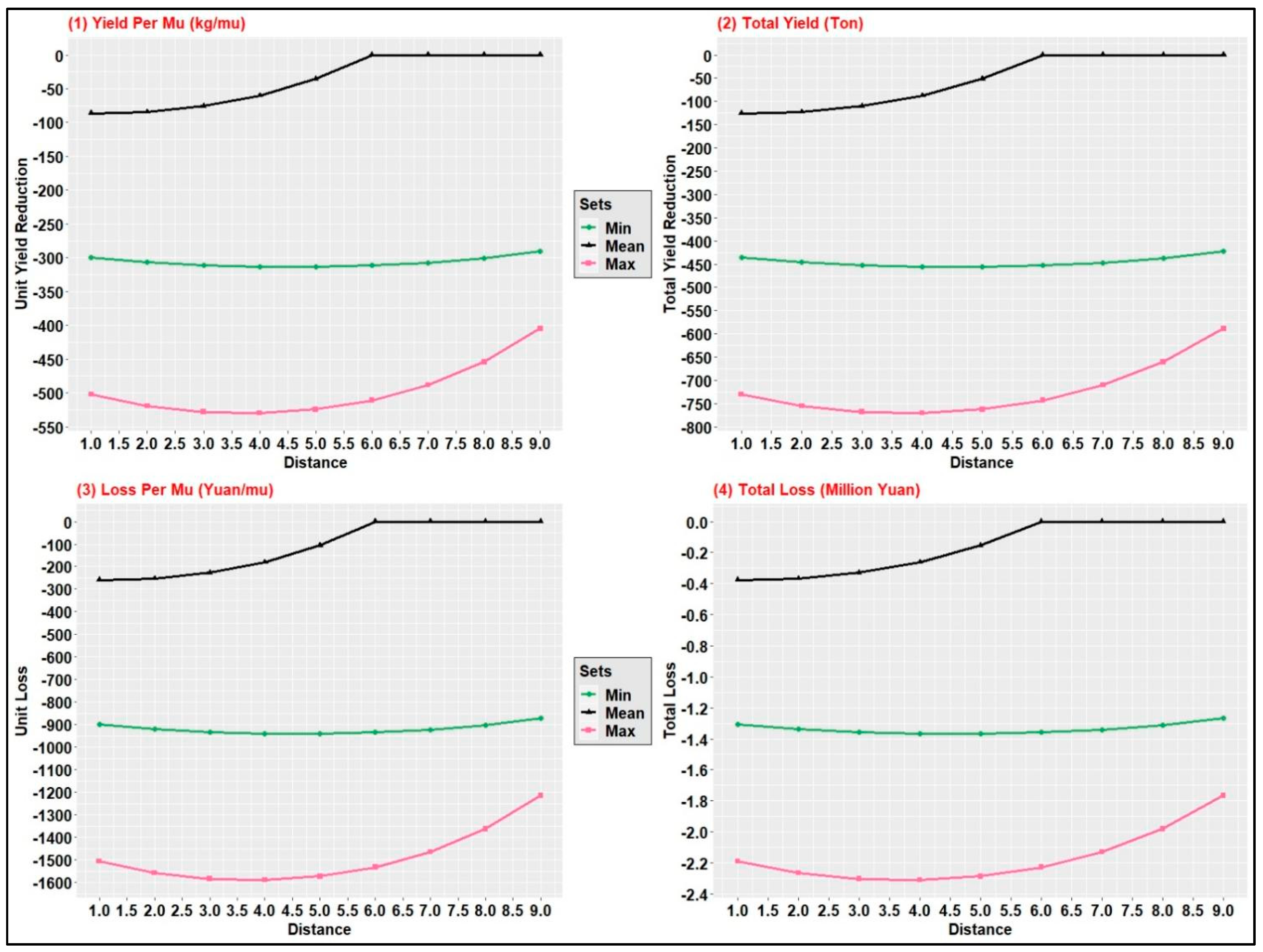
The corn outputs were estimated by inputting the values of each of the three sets into the production functions. As surveyed, the price of corn at local market was 3 Yuan kg−1 and the total cultivated area of corn in the survey area is 1453.79 mu. This paper compares the differences of the three sets from four aspects: yield per mu, total yield, loss per mu and total loss. The final results are shown in Figure 3.
There are two main findings here: First, the corn yield reduction and the loss are the smallest when the input of each factors takes their own average value. The maximum loss per mu is about 80 kg, and the loss per mu is about 260 yuan. Second, a decline or increase in factors’ input can expand the reduction in corn production caused by industrial air pollution, but the scenario of increasing the factors input will result in more significant reduction and loss in corn production. In summary, Figure 3 shows that the quantity loss of corn is 50–520 kg mu−1, and the corresponding economic loss was 150–1560 Yuan mu−1 for farmland with a distance of 3.67 km from the pollution source.
5. Conclusions and Policy Implication
With the increasing concerns on industrial air pollution, more research is being conducted on the impact of industrial air pollution on agriculture. However, existing literature either studied this problem from the viewpoint of biology and biophysiology, or estimated the direct agricultural economic losses resulting from industrial air pollution. There is no study on how industrial air pollution affects the agricultural output by affecting the production factors yet. This paper addressed this question by comparing the agricultural outputs in a polluted area and a non-polluted area.
The findings show that industrial air pollution resulted in a reduction of corn production. The impacts are in two ways. First, industrial air pollution reduces the output elasticity of the production factor, and significantly changes absolute amount of output elasticity. Second, industrial air pollution changes the relationship of some factors. In particular, industrial air pollution causes some factors to change from substitutable to complementary relationship, such as labor and capital, labor and chemicals, capital and seeds; and also leads to another opposite result that complementary relationship of two factors becomes substitutable, such as capital and chemicals. Considering different combinations of factors, industrial air pollution resulted in an output loss of 50–520 kg mu−1 and an economic loss of 150–1560 Yuan mu−1 for farmland with a distance of 3.67 km to the silicon industrial park.
This study presents an economic explanation of the impacts of industrial air pollution on agricultural production and enriches the literature in this field. It also provides useful information for the economic feasibility study of polluting industrial activities in agricultural areas and for making polices on the environmental protection and the design of compensation rate for agriculture. Moreover, the study can serve as a reference for understanding how industrial air pollution affects agricultural production in other places, especially when xeromorphic crops, such as wheat and sorghum, are concerned.
Author Contributions
Conceptualization, Z.W.; methodology, W.W. and Z.W.; software, W.W.; validation, W.W. and Z.W.; formal analysis, W.W. and Z.W.; investigation, Z.W.; resources, W.W. and Z.W.; data curation, W.W. and Z.W.; writing—original draft preparation, W.W.; writing—review and editing, W.W. and Z.W.; visualization, W.W.; supervision, Z.W.; project administration, W.W. and Z.W.; funding acquisition, W.W. and Z.W. All authors have read and agreed to the published version of the manuscript.
Funding
This research was funded by General Project of Humanities and Social Science Research of Henan Education Department, grant number 2021-ZZJH-046; China Postdoctoral Science Foundation, grant number 2020M672182; the National Natural Science Foundation of China, grant number 71763033, and Yunnan Planning Office of Philosophy and Social Science, grant number ZDZB201905.
Institutional Review Board Statement
Not applicable.
Informed Consent Statement
Not applicable.
Data Availability Statement
Not applicable.
Acknowledgments
We thank two anonymous referees and the editors for valuable inputs.
Conflicts of Interest
The authors declare no conflict of interest.
References
- Vlachokostas, C.; Nastis, S.A.; Achillas, C.; Kalogeropoulos, K.; Karmiris, I.; Moussiopoulos, N.; Chourdakis, E.; Banias, G.; Limperi, N. Economic damages of Ozone air pollution to crops using combined air quality and GIS modeling. Atmos. Environ. 2010, 22, 3352–3361. [Google Scholar] [CrossRef]
- Vallero, D.A. Fundamentals of Air Pollution, 4th ed.; Elsevier: Amsterdam, The Netherlands, 2014. [Google Scholar]
- Heck, W.W.; Taylor, O.C.; Tingey, D.T. Assessment of Crop Loss from Air Pollutants; Elsevier Applied Science: London, UK, 1988. [Google Scholar]
- Lee, E.H. Early detection mechanisms for tolerance and amelioration of ozone stress in crop plants. In Environmental Pollution and Plant Response; Agrawal, S.B., Agrawal, M., Eds.; Lewis Publishers: Boca Raton, FL, USA, 2000. [Google Scholar]
- Wahid, A. Influence of atmospheric pollutants on agriculture in developing countries: A case study with three new varieties in Pakistan. Sci. Total Environ. 2006, 371, 304–313. [Google Scholar] [CrossRef] [PubMed]
- Adams, R.M. Issues in assessing the economic benefits of ambient ozone control: Some examples from agriculture. Environ. Int. 1983, 9, 539–548. [Google Scholar] [CrossRef]
- World Bank. Cost of Pollution in China-Economic Estimates of Physical Damages; World Bank: Washington, DC, USA, 2007. [Google Scholar]
- Rai, R.; Agrawal, M. Evaluation of physiological and biochemical responses of two rice (Oryza sativa L.) cultivars to ambient air pollution using open top chambers at a rural site in India. Sci. Total Environ. 2008, 407, 679–691. [Google Scholar] [CrossRef] [PubMed]
- Khai, H.V.; Yabe, M. Rice yield loss due to industrial pollution in Vietnam. J. US-China Public Adm. 2012, 9, 248–256. [Google Scholar]
- Lindhjem, H.; Hu, T.; Ma, Z.; Skjelvik, J.M.; Song, G.; Vennemo, H.; Wu, J.; Zhang, S. Environmental economic impact assessment in China: Problems and prospects. Environ. Impact Assess. Rev. 2007, 27, 1–25. [Google Scholar] [CrossRef] [Green Version]
- Humblot, P.; Leconte-Demarsy, D.; Clerino, P.; Szopa, S.; Castell, J.-F.; Jayet, P.-A. Assessment of ozone impacts on farming systems: A bio-economic modeling approach applied to the widely diverse French case. Ecol. Econ. 2013, 85, 50–58. [Google Scholar] [CrossRef]
- Ishii, S.; Bell, J.N.B.; Marshall, F.M. Phytotoxic risk assessment of ambient air pollution on agricultural crops in Selangor State, Malaysia. Environ. Pollut. 2007, 150, 267–279. [Google Scholar] [CrossRef] [PubMed]
- Dixon, B.L.; Garcia, P.; Mjelde, J.W.; Adams, R.M. Estimation of the Economic Cost of Ozone on Illinois Cash Grain Farms; Final Report to USEPA, Corvallis Environmental Research Laborator; University of Illinois Agricultural Experiment Station: Urbana, IL, USA, 1983. [Google Scholar]
- Ye, H.; Ma, W.; Yang, B.; Ren, J.; Liu, D.; Dai, Y. The lifecycle assessment of industrial silicon. Light Met. 2007, 11, 46–49. [Google Scholar]
- Aragon, F.M.; Rud, J.P. Modern Industries, Pollution and Agricultural Productivity: Evidence from Ghana. Working Paper. 2013. Available online: https://www.theigc.org/wp-content/uploads/2014/09/Aragon-Rud-2013-Working-Paper.pdf (accessed on 15 May 2021).
- Shankar, B.; Neeliah, H. Tropospheric ozone and winter wheat production in England and Wales: A note. J. Agric. Econ. 2005, 56, 145–151. [Google Scholar] [CrossRef]
- Neeliah, H.; Shankar, B. Ozone pollution and farm profits in england and wales. Appl. Econ. 2010, 42, 2449–2458. [Google Scholar] [CrossRef] [Green Version]
- Blanenau, W.F.; Cassou, S.P. Industry estimates of the elasticity of substitution and the rate of biased technological change between skilled and unskilled labour. Appl. Econ. 2011, 43, 3129–3142. [Google Scholar] [CrossRef]
- Lin, B.; Fei, R. Analyzing inter-factor substitution and technical progress in the Chinese agricultural sector. Eur. J. Agron. 2015, 66, 54–61. [Google Scholar] [CrossRef]
- Bogetoft, P.; Otto, L. Benchmarking with DEA, SFA, and R; Springer: Berlin/Heidelberg, Germany, 2011. [Google Scholar]
- Hadley Wickham and Evan Miller. Haven: Import and Export ‘SPSS’, ‘Stata’ and ‘SAS’ Files. R Package Version 2.3.1. 2020. Available online: https://CRAN.R-project.org/package=haven (accessed on 15 May 2021).
- Henningsen, A. Introduction to Econometric Production Analysis with R; Draft Version; University of Copenhagen: Copenhagen, Denmark, 2014. [Google Scholar]
- Paul, W. Wilson. FEAR 1.0: A Software Package for Frontier Efficiency Analysis with R. Socio Econ. Plan. Sci. 2008, 42, 247–254. [Google Scholar]
- Cobb, C.W.; Douglas, P.H. A Theory of Production. Am. Econ. Rev. 1928, 18, 139–165. [Google Scholar]
- Coelli, T.J.; Rao, D.S.P.; Donnell, C.J.; Battese, G.E. An Introduction to Efficiency and Productivity Analysis; Springer Science and Business Media: New York, NY, USA, 2005. [Google Scholar]
- Kumbhakar, S.C.; Lovell, C.A.K. Stochastic Frontier Analysis; Cambridge University Press: Cambridge, UK, 2000. [Google Scholar]
- Spash, C.L. Assessing the economic benefits to agriculture from air pollution control. J. Econ. Surv. 1997, 11, 47–70. [Google Scholar] [CrossRef]
- White, H. A heteroskedasticity-consistent covariance matrix estimator and a direct test for heteroskedasticity. Econometrica 1980, 48, 817–838. [Google Scholar] [CrossRef]
Figure 1.
The output elasticity of K along with the changes of D in three models.

Figure 2.
Elasticity of substitution between factors in two groups.

Figure 3.
The economic loss of crop production.


Table 1.
Descriptive statistical analysis.
| Variable | Reference Group | Polluted Group | |||||
|---|---|---|---|---|---|---|---|
| Description | Abbr. | Sample | Mean | Standard Deviation | Sample | Mean | Standard Deviation |
| Output (kg mu−1) | Y | 160 | 289.96 | 102.07 | 146 | 239.43 | 81.36 |
| Farmland area (mu hh−1) | - | 157 | 4.37 | 3.75 | 145 | 6.04 | 4.95 |
| Labor input (man·day mu−1) | L | 159 | 18.67 | 5.94 | 145 | 15.07 | 5.28 |
| Capital input (Yuan mu−1) | K | 162 | 67.95 | 17.17 | 168 | 55.75 | 25.82 |
| Seed input (Yuan mu−1) | S | 157 | 3.23 | 1.98 | 123 | 4.51 | 4.68 |
| Chemicals’ input (Yuan mu−1) | C | 160 | 155.59 | 72.76 | 146 | 139.81 | 49.37 |
| Respondent’s sex (M = 1, F = 0) | Z1 | 165 | 0.48 | 0.50 | 158 | 0.73 | 0.45 |
| Respondent’s education attainment (year) | Z2 | 165 | 5.78 | 2.87 | 158 | 5.67 | 2.61 |
| No. of household member (person) | Z3 | 165 | 4.28 | 1.60 | 158 | 4.64 | 1.58 |
| Distance (from farmland to silicon park (km) | D | - | - | - | 158 | 3.67 | 1.99 |
| Ave. annual income (Yuan) | - | 165 | 7393.33 | 3584.03 | 158 | 7362.02 | 3927.79 |
| Respondent’s age (year) | - | 165 | 46.67 | 11.72 | 158 | 46.71 | 12.20 |
Note: 1 ha = 15 mu.
Table 2.
Estimated production functions.
| Variable and Statistics | Model I (Pooled Data) | Model II (Reference Group) | Model III (Polluted Group) | |||
|---|---|---|---|---|---|---|
| Coefficient | Std. Err. | Coefficient | Std. Err. | Coefficient | Std. Err. | |
| (1)lnL | −2.209 *** | 0.593 | −2.906 *** | 0.944 | −0.347 | 0.914 |
| (2)lnK | −2.104 *** | 0.472 | −1.456 *** | 0.560 | 2.261 | 1.580 |
| (3)lnC | 2.402 *** | 0.610 | 2.357 ** | 1.017 | 1.447 | 0.934 |
| (4)lnS | −0.291 | 0.306 | −0.957 * | 0.539 | 0.324 | 0.326 |
| (11)lnL*lnL | 0.190 *** | 0.070 | 0.175 | 0.129 | 0.102 * | 0.061 |
| (22)lnK*lnK | 0.161 *** | 0.051 | 0.109 * | 0.066 | −0.022 | 0.171 |
| (33)lnS*lnS | −0.297 *** | 0.052 | −0.276 *** | 0.075 | 0.016 | 0.106 |
| (44)lnC*lnC | 0.043 *** | 0.013 | 0.0907 *** | 0.023 | −0.006 | 0.011 |
| (12)lnL*lnK | 0.178 | 0.140 | 0.291 | 0.202 | −0.360 * | 0.205 |
| (13)lnL*lnS | 0.163 * | 0.092 | 0.250 | 0.158 | 0.327 ** | 0.140 |
| (14)lnL*lnC | −0.172 *** | 0.049 | −0.190 ** | 0.088 | −0.045 | 0.050 |
| (23)lnK*lnS | 0.014 | 0.081 | −0.016 | 0.121 | −0.383 * | 0.225 |
| (24)lnK*lnC | 0.055 | 0.079 | 0.113 | 0.128 | 0.075 | 0.071 |
| (34)lnS*lnC | 0.074 * | 0.044 | 0.182 *** | 0.064 | −0.125 * | 0.071 |
| (1)lnL*D | 0.003 | 0.003 | −0.043 | 0.030 | ||
| (2)lnK*D | 0.0158 *** | 0.004 | 0.126 ** | 0.054 | ||
| (3)lnS*D | 0.0132 *** | 0.003 | −0.114 *** | 0.041 | ||
| (4)lnC*D | 0.005 *** | 0.001 | 0.021 * | 0.012 | ||
| D | 0.020 | 0.016 | 0.094 | 0.264 | ||
| D*D | −0.005 *** | 0.000 | 0.016 *** | 0.006 | ||
| Z1 | 0.019 | 0.016 | 0.0423 * | 0.025 | 0.009 | 0.013 |
| Z2 | −0.004 | 0.003 | −0.009 * | 0.005 | 0.004 | 0.003 |
| Z3 | 0.011 ** | 0.005 | 0.011 | 0.007 | 0.009 ** | 0.004 |
| Constant | 6.252 *** | 1.725 | 5.061 * | 2.586 | −3.531 | 4.485 |
| Wald chi2 | 1837.32 (p = 0.0000) | 586.73 (p = 0.0000) | 3482.30 (p = 0.0000) | |||
| Log likelihood | 186.48 | 80.94 | 166.23 | |||
| Observations | 279 | 158 | 122 | |||
Standard errors in parentheses *** p < 0.01, ** p < 0.05, * p < 0.1.
Table 3.
The set of inputs for the estimation of corn outputs.
| Set | Labor (Man·Day mu−1) | Capital (Yuan mu−1) | Seed (Yuan mu−1) | Chemicals (Yuan mu−1) | Education (Year) | No. of HH Members (Person) | Distance (km) |
|---|---|---|---|---|---|---|---|
| Minimum value | 5 | 10 | 0.38 | 48 | 0 | 1 | 1~9 |
| Mean | 17.14 | 67.62 | 3.79 | 120.2 | 5.70 | 4.46 | 1~9 |
| Maximum value | 37 | 106 | 43.75 | 600 | 16 | 12 | 1~9 |
Publisher’s Note: MDPI stays neutral with regard to jurisdictional claims in published maps and institutional affiliations. |
© 2021 by the authors. Licensee MDPI, Basel, Switzerland. This article is an open access article distributed under the terms and conditions of the Creative Commons Attribution (CC BY) license (https://creativecommons.org/licenses/by/4.0/).
Share and Cite
MDPI and ACS Style
Wei, W.; Wang, Z. Impact of Industrial Air Pollution on Agricultural Production. Atmosphere 2021, 12, 639. https://0-doi-org.brum.beds.ac.uk/10.3390/atmos12050639
AMA Style
Wei W, Wang Z. Impact of Industrial Air Pollution on Agricultural Production. Atmosphere. 2021; 12(5):639. https://0-doi-org.brum.beds.ac.uk/10.3390/atmos12050639
Chicago/Turabian StyleWei, Wei, and Zanxin Wang. 2021. "Impact of Industrial Air Pollution on Agricultural Production" Atmosphere 12, no. 5: 639. https://0-doi-org.brum.beds.ac.uk/10.3390/atmos12050639
Note that from the first issue of 2016, this journal uses article numbers instead of page numbers. See further details here.