Using Copernicus Atmosphere Monitoring Service (CAMS) Products to Assess Illuminances at Ground Level under Cloudless Conditions

Abstract

Natural daylight is recognized as an important variable in the energy performance of buildings. A method that estimates the global illuminance received on a horizontal surface at ground level and its direct component at normal incidence under cloudless conditions is presented. The method uses the k-distribution method and the correlated-k approximation to compute a set of clearness indices integrated over 13 spectral bands covering the range 380–780 nm. A spectral resampling technique, including a spectral disaggregation and a spectral linear interpolation, is applied to these indices for providing a detailed set of solar irradiances at 1 nm in spectral resolution over the whole range. Then, these are weighted by the standardized CIE action spectrum for human eye for assessing the illuminance. Inputs to the method include the total column contents of ozone and water vapor as well as aerosol optical properties produced by the Copernicus Atmosphere Monitoring Service. Estimates of illuminance were compared to high-quality 1 min measurements of illuminance that were collected from two experimental sites located in two different climatic zones. A slight overestimation is observed for the global illuminance: the bias is between +1 klx and +3 klx, i.e., between +1% and +4% in relative value. The root mean square error varies between 5 klx (8%) and 6 klx (9%). The squared correlation coefficient ranges between 0.95 and 0.97. At the site providing the direct illuminance at normal incidence, the performance of the method is lower compared to global illuminance with a lower squared correlation coefficient of 0.53. The bias, relative bias, RMSE, and rRMSE are +7 klx, +9%, 12 klx, and 15%, respectively. The uncertainty of the method is of the order of the uncertainty of the measurements. The method offers accurate estimates of illuminance in cloudless conditions at high spatial and temporal resolutions useful for construction industries and operators as well as thermal simulation tools for optimal building design strategies.

1. Introduction

Natural daylight radiation reaching the surface of the Earth has become an essential climatic variable in the human daily life. For instance, daylight radiation is well known as the primary source of our visual and thermal comfort. The maximal usage of daylight radiation in building design strategies contributes to the reduction of energy consumption to the optimal sizing of cooling and heating units [1]. In that sense, European directives on the cost-optimal levels of energy performance of buildings press and urge construction industries and operators to use natural daylight radiation [2]. These strict regulations have yielded, year after year, to a growing need of spatial and temporal availability of natural daylight radiation data [3,4].

A very popular quantity to determine the level of natural daylight radiation is the illuminance. It is a measure of the incident flux per unit surface, which is spectrally weighted by the standardized action spectrum for human eye over the spectral range between 380 and 780 nm. Illuminance is expressed in lx. The International Commission on Illumination abbreviated as CIE according to its French acronym (Commission Internationale de l’Eclairage) has established several spectral responses of human visual perception of brightness. The 1988 spectrum is the most recent and widely used [5]. The luminous efficacy characterizes the level of daylight radiation: it is defined as the ratio of the illuminance to the total solar irradiance (W m⁻²) received at ground level and is expressed in (lm W⁻¹).

The most reliable mean to monitor the illuminance reaching the surface of the Earth are ground-based instruments. Unfortunately, ground-based stations equipped with such instruments and providing high-quality illuminance measurements are extremely sparse in the world and over time due to costs of the devices, operations, and maintenance. To overcome this paucity, researchers and practitioners have developed methods to estimate the illuminance from the broadband irradiance, i.e., the downwelling solar irradiance received at surface measured by pyranometers from 280 to 2800 nm, since there are much more stations measuring the latter or it can be assessed at any place from satellite images ([6,7]). Several empirical relationships have been published (see e.g., [8,9]), which differ in form and parameters and whose results are strongly dependent on other meteorological variables and/or sky conditions.

Another way to obtain accurate estimates of illuminance is the utilization of an appropriate radiative transfer model (RTM) combined with accurate atmospheric variables as inputs as well as ground properties at a given location. libRadtran is such a RTM ([10,11]). RTMs are computationally expensive. Hundreds of detailed spectral calculations are required to estimate the illuminance at a given time at a given location. Several schemes have been published aiming at reducing the amount of computations. Among those available in libRadtran including Doubling Adding KNMI (Koninklijk Nederlands Meteorologisch Instituut) Royal Netherlands Meteorological Institute (DAK), Rapid Radiative (RAPRAD) transfer, and SPECMAGIC models, are the k-distribution method and correlated-k approximation elaborated by Kato et al. [12]. This scheme is originally designed for the calculation of the total solar irradiance, i.e., the irradiance integrated between 240 and 4606 nm. Only 32 spectral calculations are needed to estimate the total irradiance. The McClear clear-sky model [13,14] is an example of the operational use of the Kato et al. [12] scheme combined with inputs from the Copernicus Atmosphere Monitoring Service (CAMS) for computing total irradiances under cloudless conditions. It accurately reproduces the irradiance computed by libRadtran in a much faster way by using pre-computed abaci, which are also known as look-up tables, for each of the 32 spectral bands and the band 240–4606 nm, combined with interpolation functions. Hereafter, these 32 spectral bands are named Kato bands and abbreviated KB with the number in subscript. Thirteen KBs cover the whole daylight spectral range from 380 nm to 780 nm: KB₆ 363–408 nm, KB₇ 408–452 nm, KB₈ 452–518 nm, KB₉ 518–540 nm, KB₁₀ 540–550 nm, KB₁₁ 550–567 nm, KB₁₂ 567–605 nm, KB₁₃ 605–625 nm, KB₁₄ 625–667 nm, KB₁₅ 667–684 nm, KB₁₆ 684–704 nm, KB₁₇ 704–743 nm and KB₁₈ 743–791 nm.

Wandji Nyamsi et al. [15] compared the direct and global clearness indices calculated by the Kato et al. [12] scheme in each of the 32 KBs to those resulting from detailed spectral calculations made by two RTMs, including libRadtran. The clearness index KT is the ratio of the irradiance to the equivalent extra-terrestrial irradiance and is equal to the transmissivity of the atmosphere if there is no reflection by the ground. The comparison was carried out for a set of 200,000 realistic atmospheres and clouds. The authors concluded that the Kato et al. [12] scheme is accurate and useful for representing clearness indices in each of the 13 KBs covering the daylight radiation under cloudless and cloudy sky conditions. Hence, the combination of the Kato et al. [12] scheme and inputs from CAMS is a good candidate for an accurate estimation of the illuminance.

Nevertheless, the KBs do not precisely overlay the daylight spectral range. A technique has been developed to overcome this issue and to take into account the CIE standardized action spectrum. This paper describes the method to derive the illuminance from the clearness indices in the 13 KBs, which are themselves calculated from runs of libRadtran with inputs from CAMS. The method is not entirely new, since it has already been experimented in the case of UV fluxes using the most improved version of absorption parametrization included in libRadtran and named katoandwandji ([16,17]) and photosynthetically active radiation (PAR) [18,19], but it has never been tested in the case of illuminance nor in combination with a spectral response. This study is part of an extensive project whose overarching goal is to freely and publicly offer datasets of illuminance at any time and any location in an operational way similar to the McClear model [13,14] with inputs on atmosphere variables originating from CAMS. To achieve this project, a step-by-step approach was adopted in which the performance of the clear-sky procedure is separately assessed to be better able to later understand the performance of the modelling of the cloud effects. The accuracy of the presented method is evaluated at two sites providing high-quality 1-min measurements of illuminance under cloudless conditions. Overall, this study contributes to answering the growing need of construction industries and investors on the spatial and temporal availability of illuminance at ground level for optimal building design strategies.

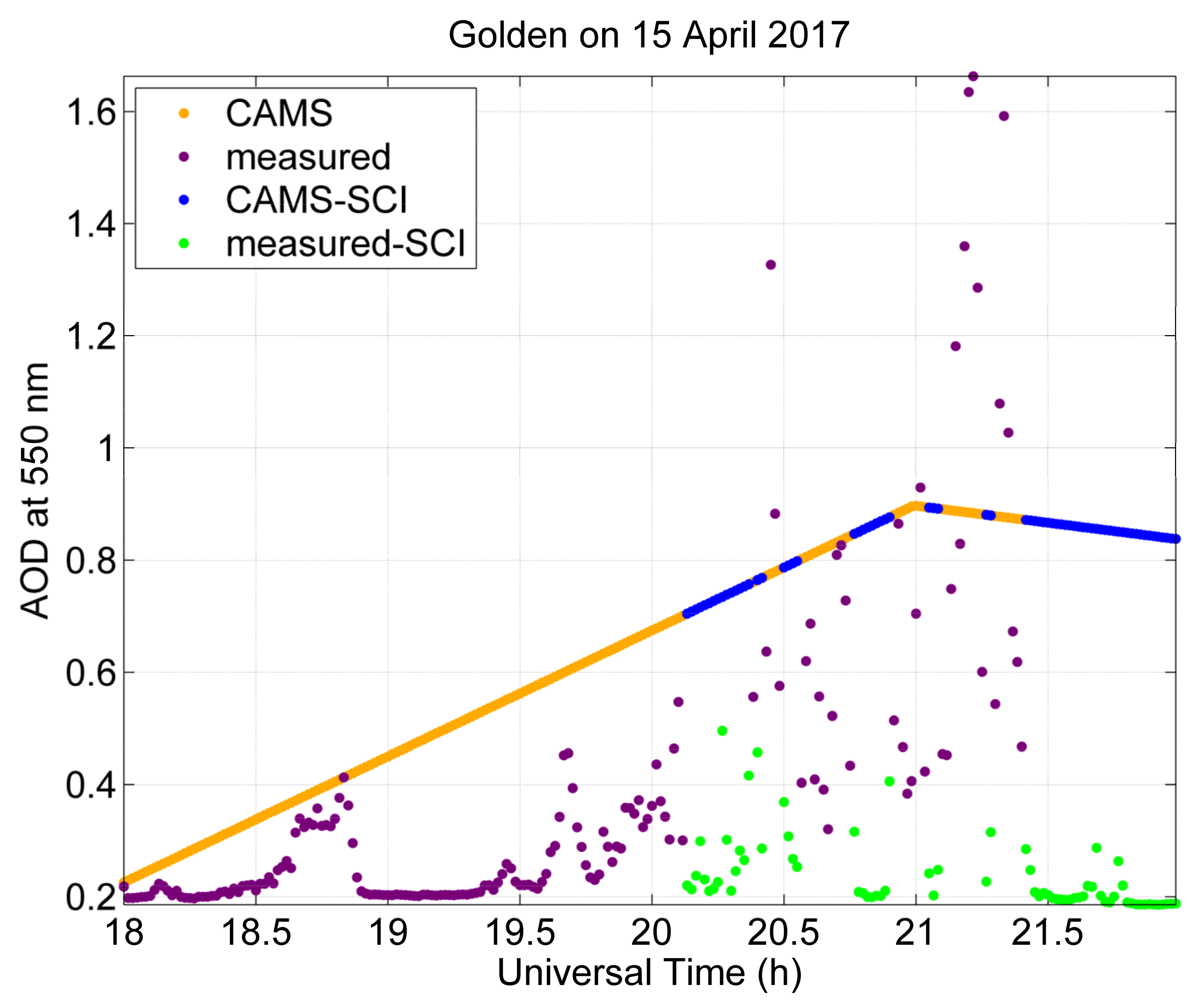
2. Description of Measurements Used for the Validation

Measurements of illuminance used for validation were collected from two stations: Vaulx-en-Velin and a station of National Renewable Energy Laboratory (NREL) in Golden, Colorado, located in France and the United States, respectively.

Table 1. Description of stations used for validation.

Station	Country	Lat. (°)	Long. (°)	Altitude a.s.l (m)	CAMS Mean Altitude (m)	Period
Vaulx-en-Velin	France	45.78	4.92	170	634	1 January 2006 to 30 June 2020
Golden, CO	United States	39.74	−105.18	1829	2200	5 May 2005 to 31 December 2019

gives the geographical coordinates, the altitude of the CAMS cell containing the station from which atmospheric inputs are extracted, and the temporal period of measurements. At both stations, measurements are illuminances provided every minute. The station of Vaulx-en-Velin is located in the eastern part of Lyon urban community and is part of the International Daylight Measurement Program network of the CIE. The environment surrounding the station is made up of 70% urban housing and 30% of cultivated fields and parks. The climate is temperate with a maritime influence. Diffuse and global illuminances on horizontal surface were measured by two independent LMT BAP 30 FCT photometric sensors. One of these sensors is equipped with a shadow ring for measuring the diffuse component. The relative uncertainty of the global or diffuse illuminance is estimated at 5% ([20]). These measurements are freely/publicly accessible and can be downloaded from the website http://idmp.entpe.fr/mesfr.htm, last access: 1 December 2020.

The direct illuminance at normal incidence L_BN is derived from the global and diffuse illuminances L_G and L_D measured on a horizontal surface as follows:

$$L_{BN}^{}=\frac{L_G-L_D}{\mathit{cos}\left({Ɵ}_s\right)}$$

(1)

where ϴ_s is the solar zenith angle, which is calculated with the SG2 algorithm [21].

The station at Golden is a high–altitude site experiencing a quite dry climate located in the Colorado state of the United States. The station field is flat and is covered by natural grasses without trees. Only measurements of the global illuminance on a horizontal surface were available and measured by a Global Photometric sensor model LI-210. These measurements have been downloaded from the website midcdmz.nrel.gov/apps/sitehome.pl?site=BMS, accessed on 1 December 2020. The relative uncertainty of the measurements is approximately 8% ([22]).

In addition, measurements of broadband diffuse and global irradiances received on a horizontal surface and of direct irradiance at normal incidence were collected at both stations with 1 min of temporal resolution. With the assumption that cloudless instants identified by scrutinizing broadband irradiances are also cloudless instants in the illuminance measurements, the three datasets of broadband irradiances have served to select the cloudless instants instead of a single dataset of global illuminance at Golden or two datasets at Vaulx-en-Velin. When applied to the time series of the broadband direct, diffuse, and global irradiances at each site, the algorithm of Lefèvre et al. [13] yields a series of detected cloudless instants. The first of the two filters in this algorithm only retains those values for which the ratio of the diffuse to the global irradiance is under 0.3. The second filter uses the product of the clearness index KT by a typical air mass and inspects the temporal variability of this quantity, which should be steady for three hours under cloudless conditions. It may happen that in certain circumstances, the illuminance may be affected by scattered cloudiness, which may go undetected in the broadband measurements. Consequently, the retained series of cloudless periods may include cloudy periods for the illuminance. Given the high selectivity of the Lefèvre et al. [13] algorithm, the authors believe that such cases are rare and that the conclusions are unaffected as a whole. An additional test rejects cloudless instants for which the measurements of the global or diffuse illuminance are less than or equal to 0.

3. Description of the Method

In a nutshell, the method applies a spectral resampling technique, including a spectral disaggregation and a spectral linear interpolation, to the 13 KB-integrated clearness indices for providing a detailed set of clearness indices at 1 nm of spectral resolution over the whole range 380–780 nm. These detailed clearness indices are converted into spectral irradiances and then weighted by the standardized CIE action spectrum for human eye for assessing the global illuminance on horizontal surface and the direct illuminance at normal incidence.

3.1. Data Exploited by Libradtran

Under cloudless conditions, illuminances at the surface level depend mostly on the solar zenithal angle ϴ_s, aerosol optical properties that may be characterized by the Angström exponent, aerosol type and aerosol optical depth (AOD), total amount of water vapor (TWV) and ozone (TOC), ground albedo, vertical profiles of temperature, pressure, density, volume mixing ratio for gases as a function of altitude, and altitude of the ground above mean sea level. As previously mentioned, this study participates in the development of an operational method, and the sources of data to be input to libRadtran should be chosen to ease the estimation of illuminance at any location and any time. A convenient way to fulfill this operational constraint is the exploitation of the atmospheric products delivered by CAMS. The SoDa service (http://www.soda-pro.com/, accessed on 1 December 2020) provides an access to the CAMS aerosol optical properties together with TOC and TWV. ϴ_s is calculated with the SG2 algorithm [21]. libRadtran offers several solar spectra; that of Gueymard [23] was selected for computing the solar spectral irradiance Io_Nλ received at the top of atmosphere at normal incidence at any time, λ being the wavelength. Air Force Geophysics Laboratory (AFGL) vertical profiles are used and selected at any location using the map of Gschwind et al. [14]. The Shuttle Radar Topography Mission dataset is used to extract the ground altitude.

The albedo of the ground in the daylight spectral band denotes the portion of the incident sunlight reflected by the ground in this band and is unknown in most cases. To solve this problem, it was assumed that the “daylight” albedo is equal to the PAR albedo because their spectral ranges are fairly similar. The acronym PAR stands for Photosynthetically Active Radiation, which is the part of solar radiation that lies in the wavelength range of 400–700 nm. The PAR albedo itself is assumed to be 0.47 times the broadband albedo [24]. The broadband albedo is defined as the integral of the bidirectional reflectance distribution function (BRDF), depending on the surface type and its roughness. Here, the broadband albedo is given by the series of maps of Blanc et al. [25] that provide the MODIS-derived BRDF parameters for each calendar month with no missing values at a spatial resolution of 0.05°. One-min values of the inputs listed above are conveniently retrieved by machine-to-machine requests made in the verbose mode to the McClear web service on the Soda website (Gschwind et al. [26], http://www.soda-pro.com/, accessed on 1 December 2020).

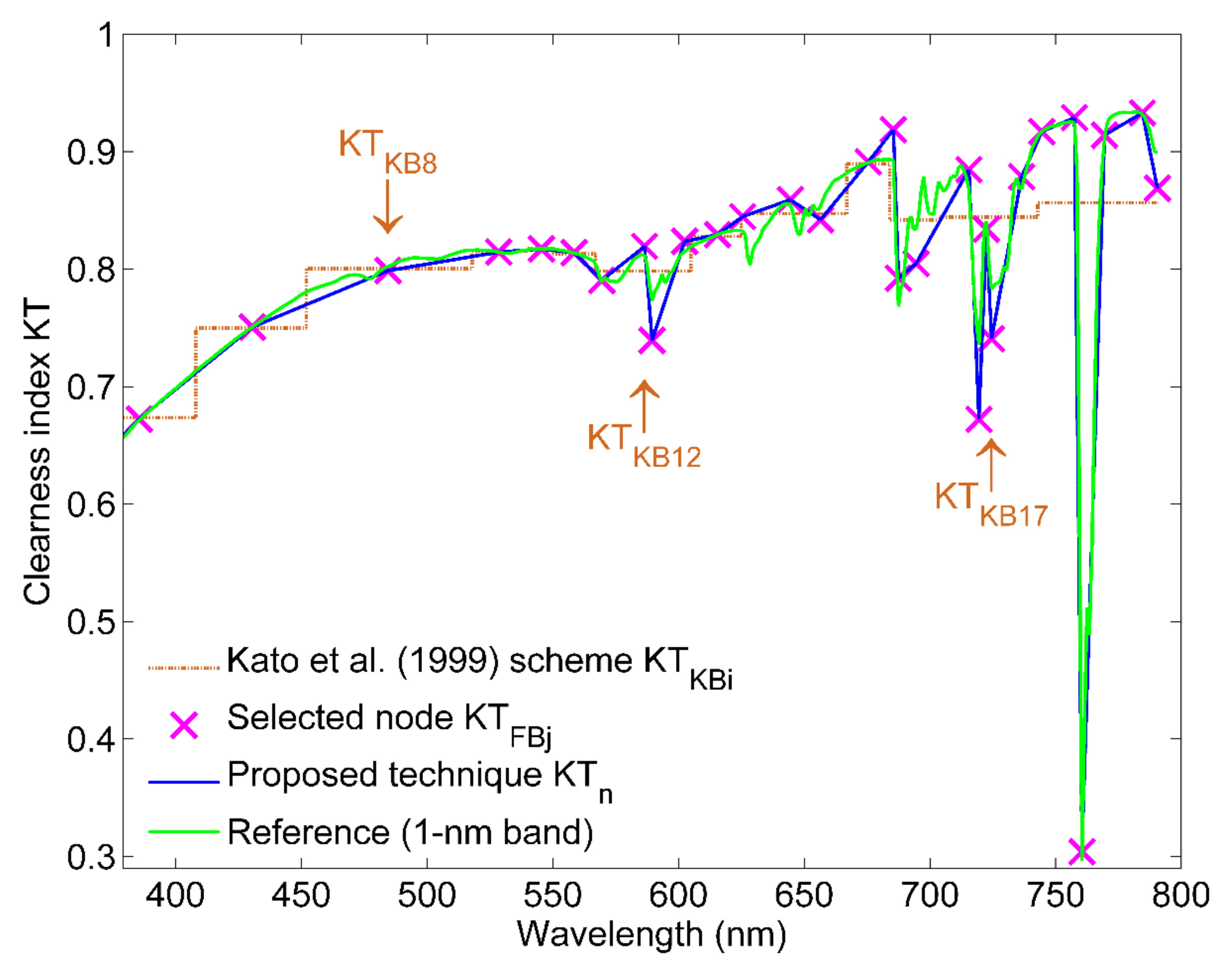
3.2. Spectral Resampling Technique

Let L_G and G_λ be the global illuminance and the global spectral irradiance received on a horizontal surface at ground level, where λ is the wavelength (in nm). L_G is given by:

$$L_G=K_{max }\underset{380}{\overset{780}{{\displaystyle \int }}}{S}_{\lambda }{G}_{\lambda } d\lambda$$

(2)

where $K_{max }$ is a constant defined as the maximum luminous efficacy and equal to 683 lm W⁻¹, and $S_{\lambda }$ is the standardized CIE action spectrum for human eye. In the same way, the direct illuminance at normal incidence L_BN is given by:

$$L_{BN}=K_{max }\underset{380}{\overset{780}{{\displaystyle \int }}}{S}_{\lambda }{B}_{N\lambda } d\lambda$$

(3)

where B_Nλ is the direct spectral irradiance at normal incidence.

Let KT_λ and KT_Bλ be the spectral clearness index and the direct clearness index. They are given by:

$$K{T}_{\lambda }=\frac{G_{\lambda }}{I{o}_{N\lambda }\mathit{cos}\left({Ɵ}_s\right)}$$

(4)

$$K{T}_{B\lambda }=\frac{B_{\lambda }}{I{o}_{N\lambda }}.$$

(5)

The libRadtran runs provide the clearness indices KT_KBi and KT_{B_KBi} in each of the 32 spectral bands. Altogether, the thirteen KBs, from KB₆ to KB₁₈, do not precisely overlay the daylight spectral range 380–780 nm, since the KB₆ 363–408 nm and KB₁₈ 743–791 nm only partially cover the daylight spectral range.

The method that has been developed overcomes this issue and takes into account the CIE standardized action spectrum. The driving idea is to find a reasonable small number of spectral bands of 1 nm in width, noted FB_j for fine band, whose spectral clearness indices KT_FBj and KT_{B_FBj} are calculated from the integrated ones in the KB_i by affine functions. This is the spectral disaggregation step. Then, a complete and detailed set of clearness indices at 1 nm of spectral resolution over the whole range 380–780 nm is obtained by a linear interpolation of these FB_j clearness indices. The 1 nm clearness indices are converted into 1 nm irradiances G_λ and B_Nλ that are then weighted by the standardized CIE action spectrum for human eye for assessing the global illuminance L_G on horizontal surface and the direct illuminance at normal incidence L_BN.

By assuming that the spectral clearness indices and the irradiances are constant over 1 nm, the integrals in Equations (2) and (3) can be approximated by finite sums, called Riemann sums. For instance, L_G and L_BN can be computed as follows:

$$L_G=K_{max }{\displaystyle \sum }_{n=380}^{780}{S}_n G_n$$

(6)

$$L_{BN}=K_{max }{\displaystyle \sum }_{n=380}^{780}{S}_n B_{Nn} .$$

(7)

or using the clearness index KT_n and the direct clearness index KT_Bn:

$$L_G=K_{max }\mathit{cos}\left({Ɵ}_s\right) {\displaystyle \sum }_{n=380}^{780}{S}_n I{o}_{Nn} K{T}_n$$

(8)

$$L_{BN}=K_{max } {\displaystyle \sum }_{n=380}^{780}{S}_n I{o}_{Nn} K{T}_{Bn} .$$

(9)

The spectral resampling technique has been described in Wandji Nyamsi et al. [16,18,19] for the UV and PAR ranges respectively and is outlined here for a better understanding. The proposed method is a pure modeling concept with radiative transfer simulations made with libRadtran. No measurements have been used for its development. First, a set of 60,000 atmospheric condition parameters under cloudless conditions has been built with Monte Carlo draws, following the statistical distribution of each input, as reported in

Table 2. KB_i covering the daylight range and selected fine bands FB_j, slopes and intercepts of the affine functions between the clearness indices in KB_i and 1 nm FB_j.

KBi	Interval Δλ, nm	Fine Band FBj, nm	Clearness Index		Direct Clearness Index
			$\mathbf{Slope} \left({\mathit{a}}_{\mathit{F}\mathit{B}\mathit{j}}\right)$	$\mathbf{Intercept} \left({\mathit{b}}_{\mathit{F}\mathit{B}\mathit{j}}\right)$	$\mathbf{Slope} \left({\mathit{c}}_{\mathit{F}\mathit{B}\mathit{j}}\right)$	$\mathbf{Intercept} \left({\mathit{d}}_{\mathit{F}\mathit{B}\mathit{j}}\right)$
6	363–408	385–386	1.0030	−0.0032	0.9987	−0.0023
7	408–452	430–431	0.9995	0.0013	1.0026	−0.0004
8	452–518	484–485	0.9979	0.0000	1.0034	0.0005
9	518–540	528–529	1.0008	−0.0013	0.9998	−0.0005
10	540–550	545–546	1.0003	−0.0003	1.0001	0.0003
11	550–567	558–559	0.9997	0.0012	1.0004	0.0004
		569–570	1.0024	−0.0100	0.9960	−0.0119
12	567–605	586–587	0.9929	0.0267	1.0123	0.0064
		589–590	0.9804	−0.0434	0.9568	−0.0109
		602–603	1.0051	0.0212	1.0150	0.0167
13	605–625	615–616	0.9977	0.0033	1.0004	0.0009
		625–626	1.0622	−0.0551	1.0104	−0.0174
14	625–667	644–645	0.9960	0.0154	1.0072	0.0029
		656–657	0.9698	0.0205	0.9915	0.0068
15	667–684	675–676	0.9978	0.0036	1.0006	0.0007
		685–686	0.9681	0.1036	1.0473	0.0212
16	684–704	687–688	1.0041	−0.0531	0.9602	−0.0130
		694–695	1.0323	−0.0642	0.9828	−0.0153
		715–716	0.9771	0.0596	1.0262	0.0121
		719–720	1.1197	−0.2733	0.899	−0.0704
17	704–743	722–723	1.0457	−0.0491	1.0049	−0.0118
		724–725	1.1046	−0.1921	0.9484	−0.0478
		736–737	0.9663	0.0626	1.0156	0.0212
		744–745	1.0401	0.0262	1.0629	−0.0036
		757–758	1.0169	0.0580	1.0622	0.0096
		760–761	0.7613	−0.3480	0.4914	–0.0805
18	743–791	769–770	0.9975	0.0598	1.0459	0.0137
		784–785	0.9688	0.1032	1.0492	0.0300
		790–791	1.0135	0.0008	1.0158	0.0078

in [16]. For each condition, libRadtran is run twice for both the direct and global irradiances: one with the detailed spectral calculations every 1 nm and the other with the Kato et al. [12] scheme. Then, the irradiances are converted into clearness indices in order to eliminate the influence of the daily and annual variations in ϴ_s and the solar spectrum. For both the global and direct irradiances, this ensemble of runs provides two sets of clearness indices: the detailed indices at 1 nm resolution and the indices spectrally integrated over each KBi.

For a given KBi, 2D histograms were drawn for the 1 nm clearness indices KT_n, respectively KT_Bn, and KT_KBi, respectively KT_{B_KBi}, for the range 380–780 nm. A visual inspection of each 2D histogram clearly shows a straight line with a squared correlation coefficient greater than 0.99 in all cases. Therefore, affine functions were established between the clearness indices by a least-square fitting technique. There is a considerable number of affine functions, and for operational purposes, a limited set of 29 intervals of 1 nm in width, the fine bands FBj, was selected and then used in a linear interpolation process to obtain the clearness indices at each 1 nm without losing accuracy to compute the illuminance. The current approach is empirical with no guarantee that the selected set of FBj is the optimum. It could have been possible to use some mathematical optimization tools. For each FBj in a given KBi, two affine functions have been established:

$$K{T}_{FBj}=a_{FBj} K{T}_{KBi}^{}+b_{FBj}$$

(10)

$$K{T}_{B\_FBj}=c_{FBj} K{T}_{B\_KBi}^{}+d_{FBj}$$

(11)

where the parameters a_FBj, b_FBj, c_FBj, and d_FBj are given in Table 2. These two sets of affine functions are obtained once for all. The operational method is as follows. For a given set of inputs, libRadtran with the Kato et al. [12] scheme is run to provide the set of thirteen KT_KBi and KT_B__KBi from which the set of 29 KT_FBj and KT_{B_FBj} is calculated using the affine functions. Then, KT_n and KT_Bn are estimated at each 1 nm between 380 and 780 nm using spectral linear interpolation of KT_FBj and KT_{B_FBj}. Then, this complete set of 1 nm clearness indices is converted into a set of spectral irradiances G_n and B_Nn, which in turn are multiplied by the standardized CIE action spectrum for human eye, yielding the illuminances L_G and L_BN.

Figure 1 exhibits the clearness index obtained between 363 and 791 nm by runs of libRadtran with the following inputs: ${Ɵ}_s$ of 37.56°, the midlatitude winter atmospheric profile, TOC of 305 DU, TWV of 38.74 kg m⁻², AOD of 0.22 at 550 nm for a maritime tropical aerosol model with an Ångström exponent of 1.14, ground elevation of 0 m, and surface albedo of 0.07. The graph illustrates the spectral resampling technique starting from clearness indices calculated by the Kato et al. [12] scheme (in brown) up to those at the 1 nm band (in blue). The green line is the result of the detailed calculations made at 1 nm resolution with libRadtran; it is given here to show how the clearness indices resulting from the detailed calculations and from the interpolation (blue line) are very close. A visual inspection shows that in most cases, $K{T}_{FBj}$ and KT_KBi, are approximately equal at the middle wavelength of the KB_i range. Exceptions are for KB₁₂, KB₁₄, KB₁₆, KB₁₇, and KB₁₈, where KT_n exhibits a nonlinear behavior that cannot be accounted for with a single $K{T}_{FBj}$. That is the reason for selecting more than one FB_j (magenta crosses). The linear interpolation of $K{T}_{FBj}$ (in blue line) provides a fairly accurate estimate of KT_n. Overall, the graph illustrates the high capability of the spectral resampling technique to reproduce the spectral variation of the clearness index throughout the daylight spectral band.

4. Results and Discussion

The validation of the presented method was carried out by comparing the estimates to the 1 min measurements of illuminance. The errors were as follows: estimates minus measurements, were synthetized by usual statistical quantities such as the bias (mean error), the root mean square error (RMSE), and their relative values rBias and rRMSE with respect to the average of the measurements. The squared correlation coefficient also known as the coefficient of determination (R²) was also computed.

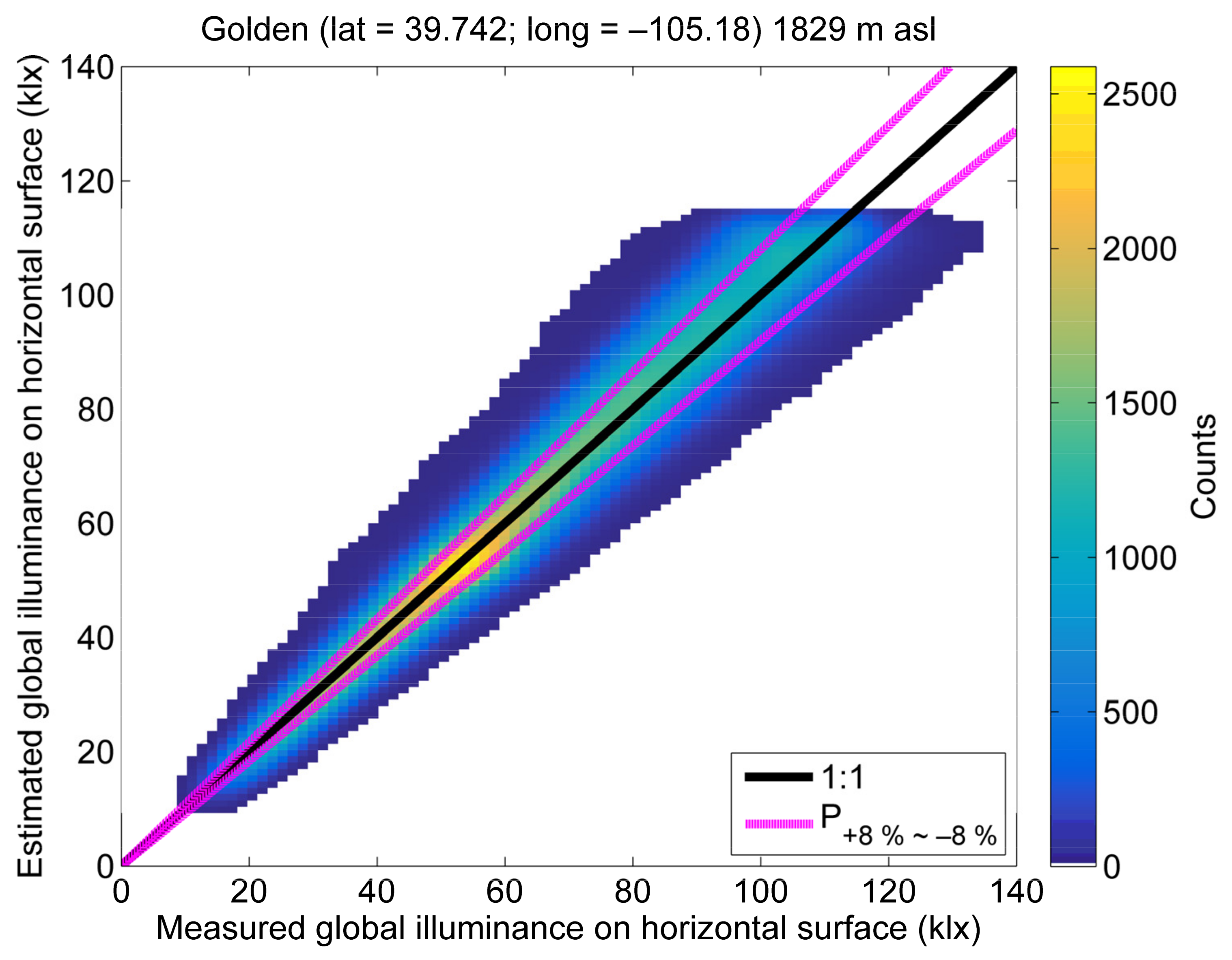
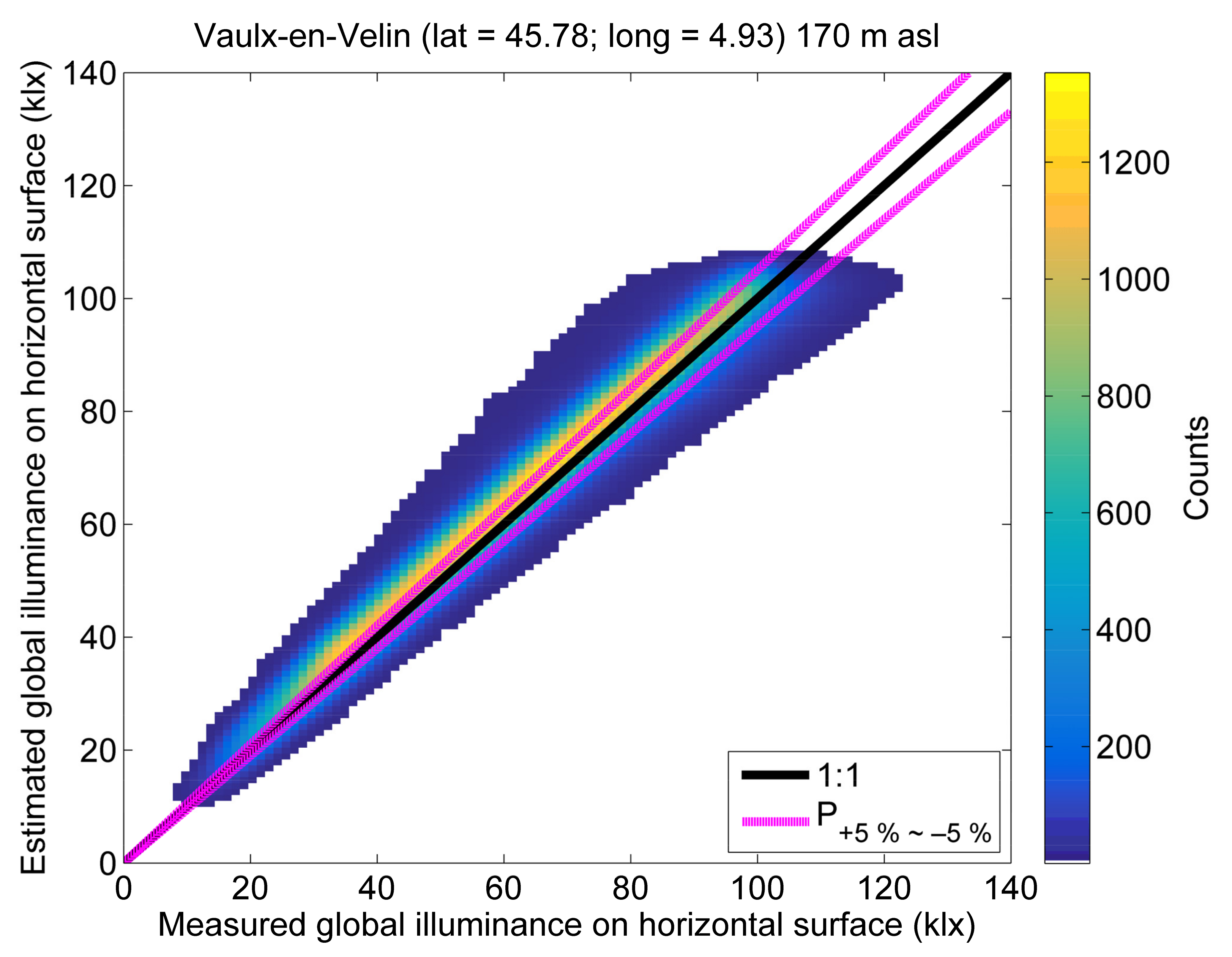
4.1. Validation on Global Illuminance on Horizontal Surface

Figure 2 exhibits the 2D histogram between 1 min measured and estimated global illuminances on horizontal surface at Golden. The 2D histogram displays the number of data pairs, also known as a count, between measured and estimated illuminances within a given bin of area 1.5 klx × 1.5 klx. Counts increase from blue to yellow. In other words, the yellower the color, the greater the count; the bluer the color, the lower the count. The cloud of points is well elongated along the 1:1 line with a limited scattering, although the spread of points increases with increasing magnitude of global illuminance.

The coefficient of determination is 0.95, denoting that more than 95% of the variability in measurements, expressed by the variance, is reproduced by the presented method. The method reveals a small positive bias and rbias of 1 klx and 1% respectively meaning a small overestimation. The RMSE is 6 klx; i.e., 9% of the average value of measurements. Statistics of errors for each station are reported in

Table 3. Statistics from the validation of the method. Mean, bias, and RMSE are expressed in (klx). rBias and rRMSE are expressed relative to the mean of the measurements. Ndata is the number of cloudless instants.

Station	Ndata	Mean	Bias	RMSE	rBias (%)	rRMSE (%)	R2
Golden	1,295,585	67	1	6	1	9	0.95
Vaulx-en-Velin	650,431	63	3	5	4	8	0.97

, together with the number of cloudless instants Ndata. With respect of the accuracy of the instrument, the method shows a good performance in assessing global illuminance on a horizontal surface. In addition, one observes that the vast majority of the points drops within the area delimited by the two thin magenta lines representing the uncertainty of the Global Photometric sensor model LI-210 estimated here to be approximately ±8% from the measurements.

In order to investigate the sources of errors, the ratio of estimated and measured global illuminances was plotted as a function of the CAMS inputs and the solar zenithal angle (ϴ_s). The investigation has been done on deviations as well. Figure 3 shows the ratio (top) and deviation (bottom) as function of ϴ_s, daylight albedo, TOC, TWV, and AOD for Golden. The dependence of the errors is graphically shown with the boxplot aiming to understand the distribution of errors and to measure the degree of dispersion and skewness of the errors for a specific interval based on a given CAMS input. The boxplot exhibits both upper and lower quartiles and the median. The results are displayed on the panels referring to one CAMS input. A boxplot is shown for a given range of values.

Overall, there is no obvious influence of the investigated inputs on the errors. An exception is made on AOD where the ratios and deviations tend to become respectively less than 1 and more negative when the AOD increases beyond 0.6. For the ratios and deviations, the magnitudes of boxes in the panel are quite small, denoting a very limited scattering of errors. These magnitudes are fairly identical in the panel of each investigated input denoting a weak influence of inputs on errors except at high AOD. Nevertheless, it is interesting to explore these strong underestimations for which AOD is greater than 0.7 in somewhat more detail.

Most of these cases occurred on 15 April 2017 between 20:08 and 22:00 UTC. Figure 4 illustrates the diurnal variability of measured and CAMS AOD at Golden over a longer period i.e., from 18:00 to 22:00 UTC. The graph provides a closer look on the temporal matching between measured and CAMS AOD. As used in this study, the original 3-h CAMS AOD has been interpolated for providing 1 min CAMS AOD estimates. For the selected cloudless instants (SCI) in this longer period, CAMS AOD (blue dot) is always much greater than the measured AOD (green dot), clearly explaining the observed strong underestimations. In addition, the graph reveals the issue of interpolated CAMS AOD, which might not adequately describe the high temporal variability of measured AOD.

Similarly to Figure 2, Figure 5 exhibits the 2D histogram at Vaulx-en-Velin. The points follow quite well the 1:1 line with a limited spread. The plot shows an overestimation close to a systematic bias. The spread of points is more limited compared to the previous case of Golden. R² is very large, up to 0.98, meaning that 98% of the variability contained in the measurements is well captured by the method. The bias is still small and is 3 kx, i.e., +4% of the average of the measurements. The RMSE is small with a value of 5 klx (8%).

At this station, the investigation of the influence of CAMS inputs on the errors yields observations that are similar to those made at Golden. In addition, the dependency of statistical quantities with the month were explored. It was found that the relative bias as well as relative RMSE are greater around the wintertime i.e., between November and February compared to other months. The sources of errors are discussed later in more details.

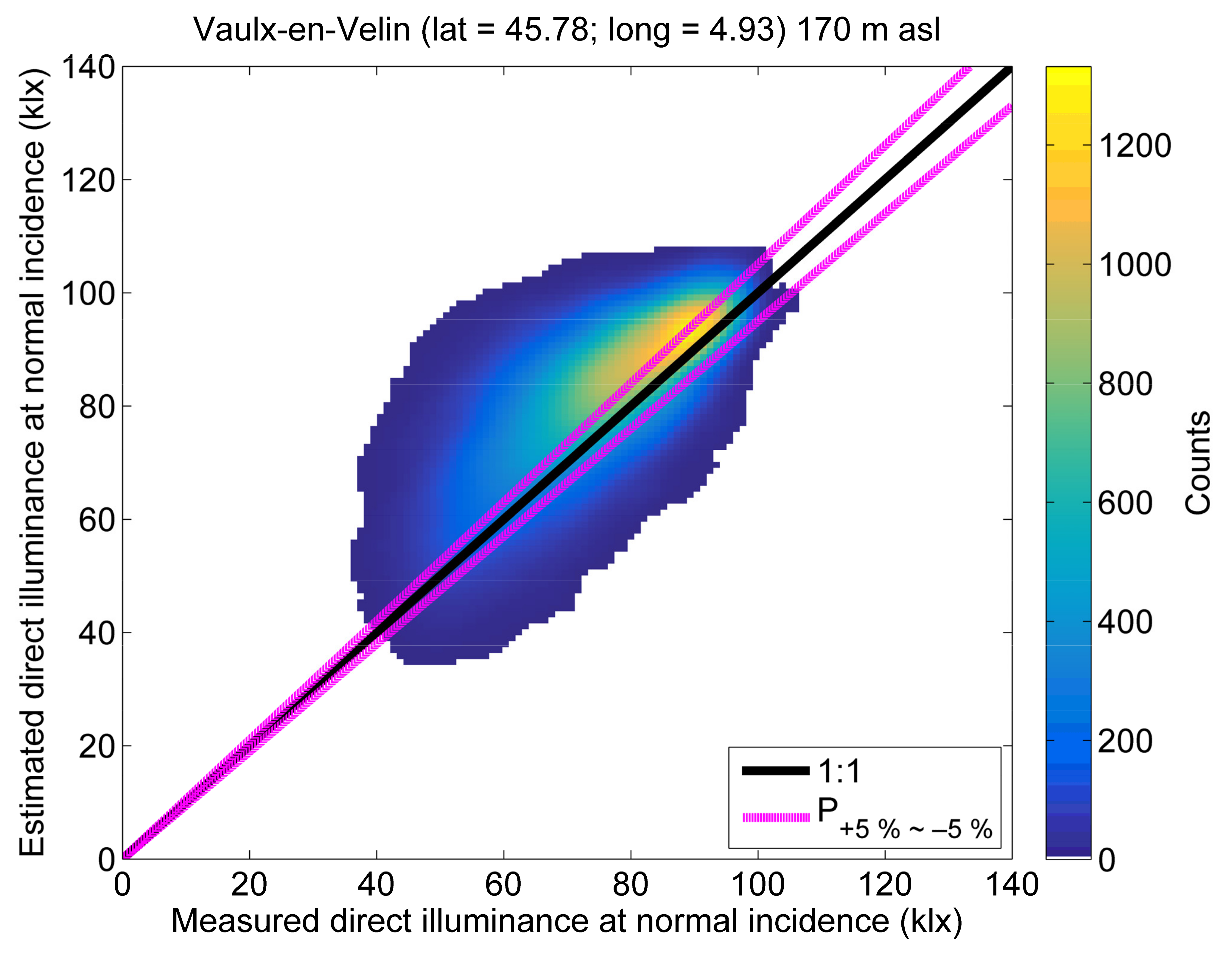
4.2. Validation on Direct Illuminance at Normal Incidence

The validation of the direct illuminance at normal incidence L_BN is only carried out at Vaulx-en-Velin. Similarly to Figure 2, Figure 6 shows the 2D histogram between measurements of L_BN and estimates for Vaulx-en-Velin while the statistics are reported in

Table 4. Same as Table 3 but for direct illuminance at normal incidence.

Station	Ndata	Mean	Bias	RMSE	rBias (%)	rRMSE (%)	R2
Vaulx-en-Velin	650,431	76	7	12	9	15	0.53

. R² is low, with a value of 0.53 denoting that the variability in L_BN is only fairly well reflected by the estimates. This small coefficient of determination may be partly explained by the restrained range of variations of the direct illuminance at normal incidence in case of cloudless conditions, and the small values do not strictly imply weaknesses in the method. The bias is 7 klx, i.e., 9% of the average of the measurements. The RMSE and rRMSE are 12 klx and 15%, respectively.

The investigations on the influence of the inputs on the errors (not shown) do not reveal an obvious dependency except for AOD at 550 nm, where the influence of aerosols is more visible in direct illuminance at normal incidence than in global illuminance. It is clearly seen that both ratio and deviation decrease from greater to less than 1 and from positive to negative respectively with increasing AOD.

The statistical quantities show that the performance of the method is worse during the period from November to February compared to other months. These observations are similar from one year to another.

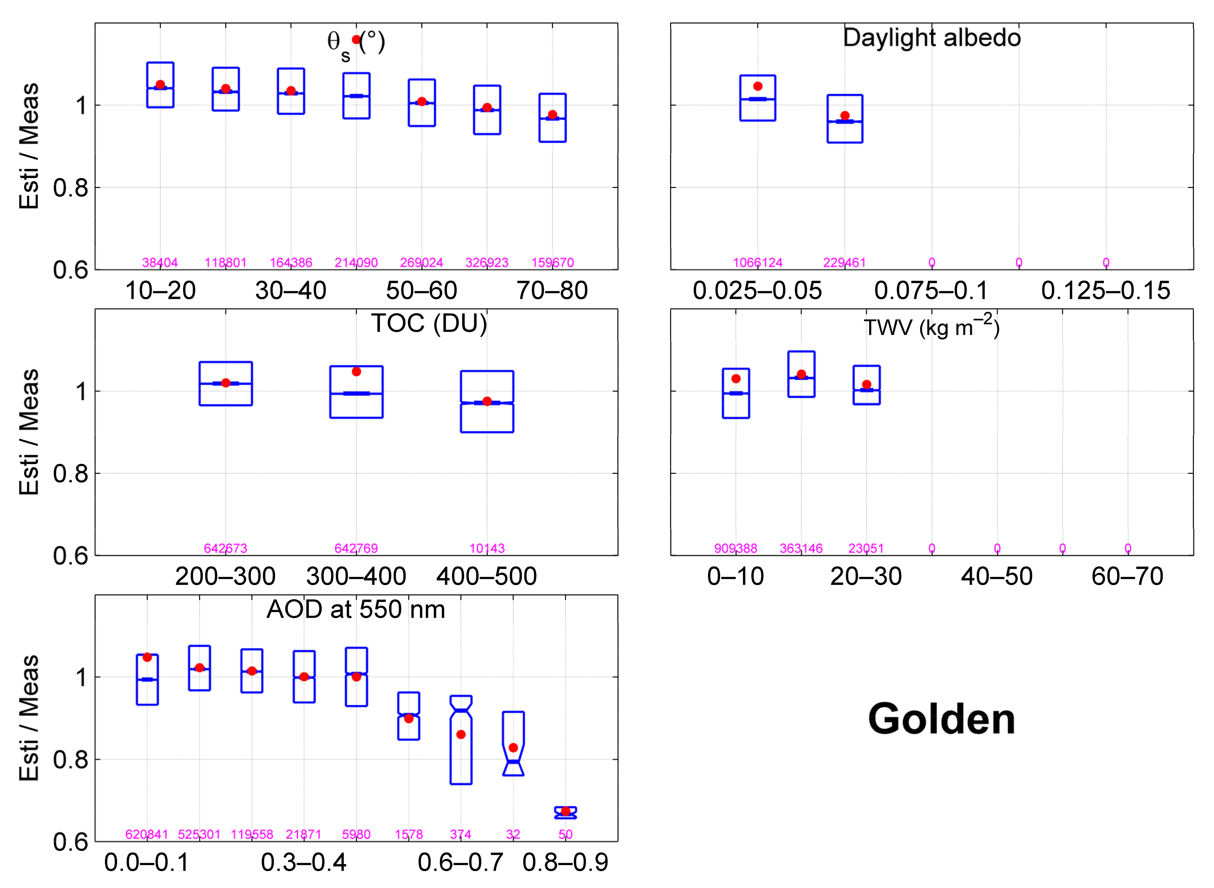
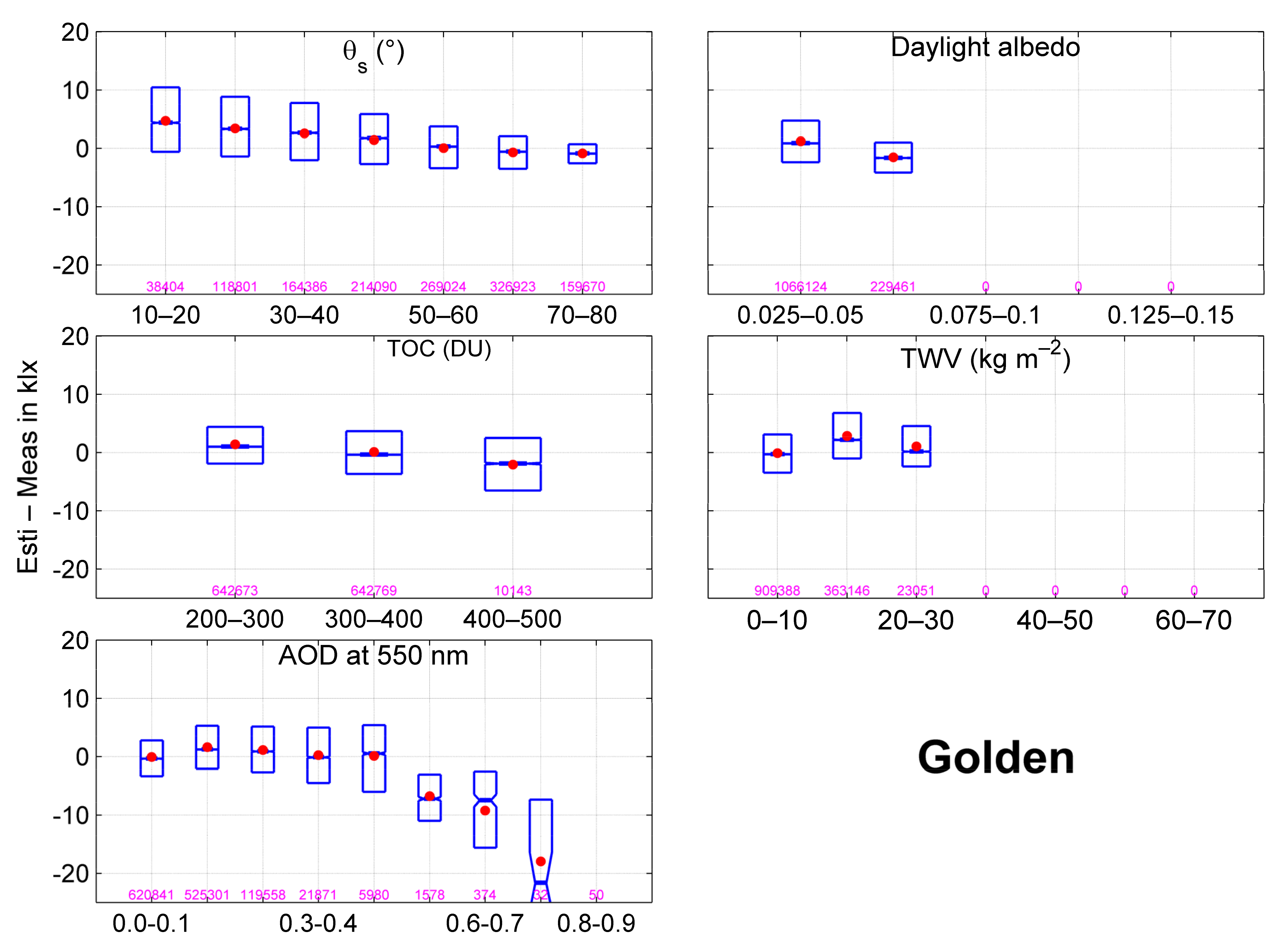
4.3. Error Analysis on Estimated Illuminances

Despite data being available at two stations only, it is worth investigating the sources of errors resulting in an overall overestimation by the presented method: slightly positive bias on the global illuminance at horizontal surface and higher positive bias on direct illuminance at normal incidence at Vaux-en-Velin. We recall that there was no measured illuminance at normal incidence. The values were derived from the measured global and diffuse illuminances at horizontal surface following Equation (1). As a positive bias is observed on validations of global illuminance, it is somehow understandable to see an overestimation on direct illuminance at normal incidence for this site. In general, four sources of errors are possible: either the main CAMS inputs, or ground albedo, or the method itself, or errors in connection with the ground-based measurements.

The accuracy of CAMS AOD and TWV were explored in more details by validating the CAMS AOD and TWV estimates to AOD and TWV measured at the closest AErosol RObotic NETwork stations. The comparison does not reveal any noticeable bias, even at the closest site Aubiere_LAMP located at 140 km. This finding is exactly in line with the worldwide performance of CAMS AOD, including Europe ([27]). The ground albedo used here reasonably represents the type of surface over year and does not exhibit any seasonality. This is confirmed by a visual analysis of images of the surface throughout the year obtained from the website: https://worldview.earthdata.nasa.gov/, accessed on 24 April 2021). Furthermore, an additional sensitivity analysis performed with libRadtran by modifying the daylight albedo does not remarkably reduce the bias. For aerosol type, “urban” and “continental average” types from OPAC (Optical Properties of Aerosols and Clouds: The Software Package OPAC, [28]) were used at Vaux-en-Velin and Golden respectively. This could affect the estimates and particularly the RMSE, as the local atmosphere may experiment other aerosol types.

An additional numerical validation was carried out by comparing the outputs of the presented method against those from detailed spectral calculations by libRadtran serving as reference to assess the accuracy of the method itself on both global illuminance at horizontal surface and direct illuminance at normal incidence. An independent sample of 10,000 atmospheric states has been randomly built following the marginal distribution variables described earlier in Section 3.2. Overall, squared correlation coefficient of 1.00 was found. In addition, both bias and RMSE (rbias and rRMSE) are less than 0.3 klx (less than 0.3%). These statistics denote the very good level of accuracy of the presented method and therefore indicate that the errors do not originate from the method itself.

It is possible that the illuminance measurements face some issues, especially at Vaux-en-Velin. However, measurements seem to be of good quality, since similar errors were found when validating both global irradiance and illuminance on the horizontal surface at this site, and since a positive bias on global irradiance on horizontal surface was also found at the close site of Payerne with the McClear model ([13]). Therefore, it might be possible that the CAMS products may not capture all atmospheric features at the regional scale particularly around Vaux-en-Velin.

5. Conclusions

A novel method for deriving the global illuminance on the horizontal surface and its direct component at normal incidence under cloudless conditions has been described here, and its accuracy has been assessed against high quality 1 min measurements. It is a preliminary and necessary step to complete an operational method for deriving illuminances in any sky conditions at any location and any time.

For global illuminance on a horizontal surface, the method exhibits a coefficient of determination greater than 0.95 at both stations, demonstrating that more than 95% of the temporal variability contained in the measurements is very well represented by the method. In general, the method exhibits a small overestimation characterized by a relative positive bias less than 5% of the average of the measurements. The relative RMSE is close to the relative bias, denoting a small standard deviation of errors. This proves a good level of performance of the presented method in assessing the global illuminance with CAMS products as inputs. The level of accuracy from the method is quite similar to the uncertainty of the measurements.

For direct illuminance at normal incidence and only limited to one station, the performance of the method is still good but less when compared to the performance for global illuminance on horizontal surface. Nevertheless, the relative bias is small. The relative RMSE is close to the relative bias denoting a limited scattering of cloud of points. As for global illuminance on a horizontal surface, this also proves the good level of accuracy of the method to estimate direct illuminance at normal incidence.

In their extensive numerical study with two RTMs, Oumbe et al. [29] observed that the influence of the cloud effects on the solar radiation received at ground level may be accurately approximated by the product of the irradiance under cloudless conditions by a cloud modification factor, which is also known as the clear-sky index. This approximation has been used at several occasions for operational computations of the broadband irradiances [30,31] or UV fluxes [32,33,34] for example. Since the proposed method delivers accurate illuminance estimates under cloudless conditions, a clear advantage is that any model assessing the influence due to clouds can be associated to this method to estimate illuminance in all-sky conditions.

References

1. Oteiza, P.; Pérez-Burgos, A. Diffuse illuminance availability on horizontal and vertical surfaces at Madrid, Spain. Energy Convers. Manag. 2012, 64, 313–319. [Google Scholar] [CrossRef] [Green Version]
2. Council, E. Directive 2010/31/EU of the European Parliament and of the Council of 19 May 2010 on the energy performance of buildings. Off. J. Eur. Union 2010, 153, 13–35. [Google Scholar]
3. Ayoub, M. 100 Years of daylighting: A chronological review of daylight prediction and calculation methods. Sol. Energy 2019, 194, 360–390. [Google Scholar] [CrossRef]
4. Galasiu, A.D.; Reinhart, C.F. Current daylighting design practice: A survey. Build. Res. Inf. 2008, 36, 159–174. [Google Scholar] [CrossRef]
5. Darula, S.; Kittler, R.; Gueymard, C.A. Reference luminous solar constant and solar luminance for illuminance calculations. Sol. Energy 2005, 79, 559–565. [Google Scholar] [CrossRef]
6. Blanc, P.; Gschwind, B.; Lefèvre, M.; Wald, L. The HelioClim project: Surface solar irradiance data for climate applications. Remote Sens. 2011, 3, 343–361. [Google Scholar] [CrossRef] [Green Version]
7. Lefèvre, M.; Blanc, P.; Espinar, B.; Gschwind, B.; Ménard, L.; Ranchin, T.; Wald, L.; Saboret, L.; Thomas, C.; Wey, E. The HelioClim-1 database of daily solar radiation at Earth surface: An example of the benefits of GEOSS Data-CORE. IEEE J. STARS 2014, 7, 1745–1753. [Google Scholar] [CrossRef] [Green Version]
8. López, G.; Gueymard, C.A. Clear-sky solar luminous efficacy determination using artificial neural networks. Sol. Energy 2007, 81, 929–939. [Google Scholar] [CrossRef]
9. Dieste-Velasco, M.I.; Díez-Mediavilla, M.; Alonso-Tristán, C.; González-Peña, D.; Rodríguez-Amigo, M.D.C.; García-Calderón, T. A new diffuse luminous efficacy model for daylight availability in Burgos, Spain. Renew. Energy 2020, 146, 2812–2826. [Google Scholar] [CrossRef]
10. Emde, C.; Buras-Schnell, R.; Kylling, A.; Mayer, B.; Gasteiger, J.; Hamann, U.; Kylling, J.; Richter, B.; Pause, C.; Dowling, T.; et al. The libRadtran software package for radiative transfer calculations (version 2.0.1). Geosci. Model Dev. 2016, 9, 1647–1672. [Google Scholar] [CrossRef] [Green Version]
11. Mayer, B.; Kylling, A. Technical note: The libRadtran software package for radiative transfer calculations-description and examples of use. Atmos. Chem. Phys. 2005, 5, 1855–1877. [Google Scholar] [CrossRef] [Green Version]
12. Kato, S.; Ackerman, T.; Mather, J.; Clothiaux, E. The k-distribution method and correlated-k approximation for shortwave radiative transfer model. J. Quant. Spectrosc. Radiat. Transf. 1999, 62, 109–121. [Google Scholar] [CrossRef]
13. Lefevre, M.; Oumbe, A.; Blanc, P.; Espinar, B.; Gschwind, B.; Qu, Z.; Wald, L.; Schroedter-Homscheidt, M.; Hoyer-Klick, C.; Arola, A.; et al. McClear: A new model estimating downwelling solar radiation at ground level in clear-sky conditions. Atmos. Meas. Tech. 2013, 6, 2403–2418. [Google Scholar] [CrossRef] [Green Version]
14. Gschwind, B.; Wald, L.; Blanc, P.; Lefèvre, M.; Schroedter-Homscheidt, M.; Arola, A. Improving the McClear model estimating the downwelling solar radiation at ground level in cloud-free conditions–McClear-v3. Meteorol. Z. 2019, 28, 147–163. [Google Scholar] [CrossRef]
15. Wandji Nyamsi, W.; Espinar, B.; Blanc, P.; Wald, L. How close to detailed spectral calculations is the k-distribution method and correlated-k approximation of Kato et al. (1999) in each spectral interval? Meteorol. Z. 2014, 23, 547–556. [Google Scholar] [CrossRef] [Green Version]
16. Wandji Nyamsi, W.; Pitkänen, M.; Aoun, Y.; Blanc, P.; Heikkilä, A.; Lakkala, K.; Bernhard, G.; Koskela, T.; Lindfors, A.; Arola, A.; et al. A new method for estimating UV fluxes at ground level in cloud-free conditions. Atmos. Meas. Tech. 2017, 10, 4965–4978. [Google Scholar] [CrossRef] [Green Version]
17. Wandji Nyamsi, W.; Arola, A.; Blanc, P.; Lindfors, A.V.; Cesnulyte, V.; Pitkänen, M.R.A.; Wald, L. Technical Note: A novel parameterization of the transmissivity due to ozone absorption in the k-distribution method and correlated-k approximation of Kato et al. (1999) over the UV band. Atmos. Chem. Phys. 2015, 15, 7449–7456. [Google Scholar] [CrossRef] [Green Version]
18. Wandji Nyamsi, W.; Espinar, B.; Blanc, P.; Wald, L. Estimating the photosynthetically active radiation under clear skies by means of a new approach. Adv. Sci. Res. 2015, 12, 5–10. [Google Scholar] [CrossRef] [Green Version]
19. Wandji Nyamsi, W.; Blanc, P.; Augustine, J.A.; Arola, A.; Wald, L. A new clear-sky method for assessing photosynthetically active radiation at the surface level. Atmosphere 2019, 10, 219. [Google Scholar] [CrossRef] [Green Version]
20. Dumortier, D. Mesure, Analyse et Modélisation du Gisement Lumineux. Application à l’évaluation des Performances de l’éclairage Naturel des Bâtiments. Ph.D. Thesis, Université de Savoie, Savoie, France, 1995. [Google Scholar]
21. Blanc, P.; Wald, L. The SG2 algorithm for a fast and accurate computation of the position of the Sun. Sol. Energy 2012, 86, 3072–3083. [Google Scholar] [CrossRef] [Green Version]
22. Light Measurement. Available online: https://www.licor.com/documents/3bjwy50xsb49jqof0wz4 (accessed on 1 December 2020).
23. Gueymard, C.A. The sun’s total and the spectral irradiance for solar energy applications and solar radiations models. Sol. Energy 2004, 76, 423–452. [Google Scholar] [CrossRef]
24. Bosch, J.L.; López, G.; Batlles, F.J. Global and direct photosynthetically active radiation parameterizations for clear-sky conditions. Agric. For. Meteorol. 2009, 149, 146–158. [Google Scholar] [CrossRef]
25. Blanc, P.; Gschwind, B.; Lefèvre, M.; Wald, L. Twelve monthly maps of ground albedo parameters derived from MODIS data sets. In Proceedings of the IGARSS 2014, Quebec, QC, Canada, 13–18 July 2014; pp. 3270–3272. [Google Scholar] [CrossRef]
26. Gschwind, B.; Ménard, L.; Albuisson, M.; Wald, L. Converting a successful research project into a sustainable service: The case of the SoDaWeb service. Environ. Model. Softw. 2006, 21, 1555–1561. [Google Scholar] [CrossRef] [Green Version]
27. Gueymard, C.A.; Yang, D. Worldwide validation of CAMS and MERRA-2 reanalysis aerosol optical depth products using 15 years of AERONET observations. Atmos. Environ. 2020, 225, 117216. [Google Scholar] [CrossRef]
28. Hess, M.; Koepke, P.; Schult, I. Optical properties of aerosols and clouds: The software package OPAC. Bull. Am. Meteorol. Soc. 1998, 79, 831–844. [Google Scholar] [CrossRef]
29. Oumbe, A.; Qu, Z.; Blanc, P.; Lefèvre, M.; Wald, L.; Cros, S. Decoupling the effects of clear atmosphere and clouds to simplify calculations of the broadband solar irradiance at ground level. Geosci. Model Dev. 2014, 7, 1661–1669, Corrigendum, 2014, 7, 2409. [Google Scholar] [CrossRef] [Green Version]
30. Huang, G.H.; Ma, M.G.; Liang, S.L.; Liu, S.M.; Li, X. A LUT-based approach to estimate surface solar irradiance by combining MODIS and MTSAT data. J. Geophys. Res. Atmos. 2011, 116, D22201. [Google Scholar] [CrossRef] [Green Version]
31. Qu, Z.; Oumbe, A.; Blanc, P.; Espinar, B.; Gesell, G.; Gschwind, B.; Klüser, L.; Lefèvre, M.; Saboret, L.; Schroedter-Homscheidt, M.; et al. Fast radiative transfer parameterisation for assessing the surface solar irradiance: The Heliosat-4 method. Meteorol. Z. 2017, 26, 33–57. [Google Scholar] [CrossRef]
32. Calbó, J.; Pages, D.; González, J.A. Empirical studies of cloud effects on UV radiation: A review. Rev. Geophys. 2005, 43, RG2002. [Google Scholar] [CrossRef] [Green Version]
33. Den Outer, P.N.; Slaper, H.; Kaurola, J.; Lindfors, A.; Kazantzidis, A.; Bais, A.F.; Feister, U.; Junk, J.; Janouch, M.; Josefsson, W. Reconstructing of erythemal ultraviolet radiation levels in Europe for the past 4 decades. J. Geophys. Res. Atmos. 2010, 115, D10102. [Google Scholar] [CrossRef]
34. Krotkov, N.A.; Herman, J.R.; Bhartia, P.K.; Fioletov, V.; Ahmad, Z. Satellite estimation of spectral surface UV irradiance:2. Effects of homogeneous clouds and snow. J. Geophys. Res. Atmos. 2001, 106, 11743–11759. [Google Scholar] [CrossRef]
Figure 1. Illustration of the spectral resampling technique. The clearness indices obtained between 363 and 791 nm by two runs of libRadtran are shown in green and brown respectively for detailed calculations at 1 nm resolution and for the Kato et al. [12] scheme. The selected fine bands FB are shown by crosses in magenta. The linear interpolation provides the clearness indices every 1 nm drawn in blue.
Atmosphere 12 00643 g001
Figure 2. Two-dimensional (2D) histogram between measurements and estimates of global illuminance on horizontal surface at Golden. The color bar depicts the number of points in the area of 1.5 klx × 1.5 klx. The two thin magenta lines delimit the area of relative errors of ±8% from the measurements.
Atmosphere 12 00643 g002
Figure 3. Box plots of the ratio (top) of the estimated (Esti) to the measured (Meas) global illuminance on horizontal surface and difference (bottom) between estimated and measured global illuminance on horizontal surface with CAMS input data at Golden. The mean of the box is marked with a red dot. The 1st, 2nd, and 3rd quartiles are marked with a blue line. The notch in the box shows the 95% confidence interval around the median. The number of data for a given range are reported in pink number.
Atmosphere 12 00643 g003aAtmosphere 12 00643 g003b
Figure 4. Diurnal variability of AOD at 550 nm from CAMS and measurements at Golden on 15 April 2017. SCI stands for selected cloudless instant.
Atmosphere 12 00643 g004
Figure 5. Two-dimensional (2D) histogram between measurements and estimates of global illuminance at Vaulx-en-Velin. The color bar depicts the number of points in the area of 1.5 klx × 1.5 klx. The two thin magenta lines delimit the area of relative errors of ±5 % from the measurements.
Atmosphere 12 00643 g005
Figure 6. Two-dimensional (2D) histogram between measurements and estimates of direct illuminance at normal incidence at Vaulx-en-Velin. The colorbar depicts the number of points in the area of 1.5 klx × 1.5 klx. The two thin magenta lines delimit the area of relative errors of ±5% from the measurements.
Atmosphere 12 00643 g006