Improving Air Pollutant Metal Oxide Sensor Quantification Practices through: An Exploration of Sensor Signal Normalization, Multi-Sensor and Universal Calibration Model Generation, and Physical Factors Such as Co-Location Duration and Sensor Age

Abstract

As low-cost sensors have become ubiquitous in air quality measurements, there is a need for more efficient calibration and quantification practices. Here, we deploy stationary low-cost monitors in Colorado and Southern California near oil and gas facilities, focusing our analysis on methane and ozone concentration measurement using metal oxide sensors. In comparing different sensor signal normalization techniques, we propose a z-scoring standardization approach to normalize all sensor signals, making our calibration results more easily transferable among sensor packages. We also attempt several different physical co-location schemes, and explore several calibration models in which only one sensor system needs to be co-located with a reference instrument, and can be used to calibrate the rest of the fleet of sensor systems. This approach greatly reduces the time and effort involved in field normalization without compromising goodness of fit of the calibration model to a significant extent. We also explore other factors affecting the performance of the sensor system quantification method, including the use of different reference instruments, duration of co-location, time averaging, transferability between different physical environments, and the age of metal oxide sensors. Our focus on methane and stationary monitors, in addition to the z-scoring standardization approach, has broad applications in low-cost sensor calibration and utility.

1. Introduction

1.1. Previous Gas-Phase Sensor Quantification Works

Low-cost sensors are increasingly utilized to monitor air quality in rural and urban spaces alike. Their decreased cost is generally in the $1000 range, as opposed to regulatory grade monitoring instruments, which can cost tens of thousands of dollars each. Using less expensive sensors means being able to study air quality in a variety of locations with a network of sensors with the same budget as employing one regulatory grade instrument. However, a lower cost also means lower quality data, as low-cost sensors generally rely on additional calibration methods, which can be lengthy and time-consuming. It can take up to a year to find a suitable sensor calibration model, yielding high enough data quality and low enough uncertainty. For gas phase pollutants, low-cost sensors are generally effective in elucidating spatial and temporal differences on neighborhood and regional scales alike [1,2,3,4,5].

Different types of low-cost sensors have been utilized depending on the pollutants of interest, price point, and physical setup. For ozone, one of our pollutants of interest, both metal oxide and electrochemical sensors have been studied extensively. One recent study found the differences in R² between metal oxide and electrochemical ozone sensors to be negligible, although the metal oxide sensors exhibited lower concentration limits than the electrochemical sensors, making them ideal for ambient concentrations lacking abnormally large spikes [6]. Other works have similarly shown small net gains and losses in R² and RMSE among sensor types [2,5,7,8,9], proving both electrochemical and metal oxide sensors to be effective in quantifying ozone depending on the application. Based on these previous findings, we use metal oxide sensors to quantify ozone and methane in this work.

The main drawback to low-cost sensors is their poor accuracy compared to their more expensive counterparts. Extensive in-situ field normalizations for metal oxide sensors are required to achieve more accurate concentration readings. This is typically accomplished by co-locating a low-cost instrument with a reference instrument and using machine learning techniques to match the low-cost sensor signals to the reference signals. Although artificial neural networks [10], Langmuir-type algorithms [11], and intelligent mathematical fits [12] have recently been employed, perhaps the most straightforward and one of the more commonly used is multivariate linear regression. While more complex methods may slightly outperform multivariate linear regression in goodness of fit [10], it is still widely used [1,2,3,4,5,7,10,13,14,15] and remains a less intensive yet reliable alternative, especially for reporting data quickly to stakeholders, who need to know their exposure level sooner rather than later.

1.2. Accepted Signal Normalization and Universal Calibration Methods

Although necessary to improve metal oxide sensor accuracy, the co-location process can be a burden, requiring additional time and resources. One of the most common forms of universal calibration for sensors, i.e., calibration modes that only require one sensor to be normalized with a reference instrument, is the multi-hop method, designed with mobile sensors in mind. In the first of these hops, or one-hop, a sensor is field normalized with a reference instrument. That sensor is then used as a secondary standard to calibrate the next sensor it will be co-located with. This method is typically utilized in mobile sensor networks, and this secondary co-location step is often referred to as a rendezvous. Additional hops would occur when the newly calibrated sensor meets another sensor in space and time, and is used as a tertiary standard to normalize the new sensor, and so on [16]. In multi-hop calibration schemes, the biggest challenge is error propagation, which can grow exponentially across each hop. To combat this, most multi-hop schemes have updated their calibration models from simple linear regression to other techniques, including ordinary least squares regression [17], geometric mean regression [18], and Bayesian-based methods [19]. If a reference instrument is available for prolonged periods of time, or can be moved upon request, automatic calibration techniques have also been developed to calibrate multiple sensors in real time and update their calibration models periodically [20]. Ozone is by far the most popular gas-phase pollutant to model and test these universal calibration models on; our inclusion of ozone using a low-cost metal oxide sensor will offer a direct comparison of how our models stack up against other measures.

Prior works relating to revamped calibration methods for methane focus on intelligent wireless sensor networks (WSN), where the sensors can communicate with each other directly [21,22]. While these maintenance-free, automated leak detection methods are considered cutting-edge, there is a need for universal calibration methods for low-cost sensors and simpler networks that are already in use. A previous Hannigan Lab study attempted a more elementary approach: using a single co-located pod to generate calibrations and applying that calibration to the rest of the pods. A three-step normalization process was required before exchanging the calibration among pods. First, linear regression matched the raw data for each sensor to those of the co-located pod used to generate the universal calibration model. Then, a linear regression model was used to fit the co-located pod to the reference data, and this model was applied to the rest of the pods. Finally, a simple trendline was subtracted out from each pod to make the dataset more uniform with respect to the calibrated pod [13]. We re-create this model in our study (more information in Section 2.4), which we will now refer to as the sensor-specific normalization model. As one of the only models previously tested for methane, we use it as benchmark for the goodness of fit of the new models proposed here.

1.3. Relevance of Oil and Gas

Each co-location site was located nearby oil and gas activities, and as such those activities were likely the dominant source of methane for each pod deployment described in this paper. The site in Los Angeles was less than 5 km from an active oil and gas facility, operating out of the Bandini Oilfield. This was also located just over a mile from inactive wells in the Boyle Heights Oilfield, which has the potential to release fugitive methane emissions [23]. There are over 5000 active oil wells in Los Angeles County alone [24]. To the northwest of Los Angeles in Shafter, CA, USA, the closest active well was only 1.5 km away from our sampling location, and pulled from the North Shafter oilfield. The two pod deployment sites in Colorado were each located within 400 m of an oil and gas facility. Greeley, Colorado is surrounded by over 20,000 active drilling locations, some of which are within the city limits [25]. Measurements in Wiggins, Colorado took place at a gas storage site. Both are derived from the Wattenberg Gas Field, which covers a sizeable portion of northeastern Colorado [26]. Although no drilling takes place in the City of Boulder, where our Colorado ozone measurements were procured, the closest active well is approximately 11 km and 12 km from the Boulder Campus and South Boulder Creek sites, respectively [26].

Since the sites in Colorado all pull from the same oilfield, we might expect to see somewhat similar chemical signatures from each of those two sites, although the extraction techniques and subsequent emissions at each may vary. In California, we sampled near two additional oilfields, so their specific characteristics may be different from one another as well as differing from those in Colorado. Overall, we expect the differences in methane levels to have more to do with proximity to oil and gas rather than the specific oilfields sampled near, since the distances between our monitors and the sites of interest vary a great deal across deployments.

Methane, the main component of natural gas, is emitted into the atmosphere during oil and gas production, collection, and processing [27]. This results from both direct emissions during these processes as well as fugitive emissions and leaks, which may be 60% higher than previously reported by the U.S. Environmental Protection Agency [28]. Many of the hydrocarbons released by oil and gas activities also exacerbate the production of ozone in the atmosphere, leading to smog and adverse health outcomes [29]. We will focus on these two pollutants in our analysis, as finding less-intensive ways to quantify them would be of interest to community members and other stakeholders living or working near oil and gas facilities.

1.4. Organizational Overview

We will first discuss our methods of data collection in Section 2.1 and Section 2.2, and present the linear regression models used throughout in Section 2.3. We then explain the sensor signal normalization (Section 2.4) and multi-pod calibration (Section 2.5) methods. The data analysis methods are presented in Section 2.6 before the results are shown for methane and ozone in Section 3.1.1 and Section 3.1.2, respectively. We then explore how the six calibration models studied perform under conditions where low-cost sensors tend to struggle: being co-located and deployed in different environments (Section 3.2.1) and using sensors of different ages (Section 3.2.2). After reviewing these results broadly, we shift focus to factors affecting specific calibration schemes: individual (Section 3.3) and universal (Section 3.4). Finally, we discuss our findings and the implications of this research within the field.

2. Methods

To explore several normalization and calibration approaches as well as the factors that impact their performance, we assembled data sets of simultaneous sensor signals and regulatory concentrations collected under various conditions, using some data as calibration and setting more aside as validation. Here, we leverage pre-existing data collected from 2015 to 2021 in both California and Colorado to test pre-existing calibration and standardization methods, in addition to proposing new methods. This large array of data ensured that the trends seen in calibration fits are reproducible, even under varying environmental conditions.

2.1. Overview

Low-cost air quality monitors dubbed U-Pods and Y-Pods were used for data collection. Both are built in-house by the Hannigan lab and represent two different generations of the same platform. Their specifications and a list of environmental and gas-phase sensors employed in each is described in detail by Collier-Oxandale and colleagues [13]. Briefly, a suite of metal oxide sensors is used to assess hydrocarbons (Figaro TGS 2600, 2602) and ozone (SGX MiCs-2611). Each Y-Pod is also equipped with an internal temperature and pressure sensor (SparkFun RHT03), and a humidity sensor (Bosch BMP085). Data are recorded locally and continuously approximately every ten seconds.

Various reference-grade instruments were also implemented at each calibration site (except for Wiggins, CO, USA) as listed in the timeline in Figure 1. Each calibration setup consisted of the pods stacked on top of each other within a meter of the reference instrument inlet on the roof of a one-story trailer. In California, the reference instruments were operated by South Coast Air Quality Management District and the California Air Resources Board in Los Angeles and Shafter, respectively. In Greeley, CO, USA, we made use of instruments run by the Colorado Department of Public Health and Environment. Data from Boulder, CO, USA was collected by the Hannigan Lab at the University of Colorado Boulder. The physical specifications of each reference site can be found in

Table 1. Physical specifications for co-location sites.

Location	Physical Specifications	Pod Configuration
South Boulder Creek	Ground mounted tripods, 1.5 m high	Tripod placements ~3–4 m below reference instrument inlet
Boulder Campus	Roof or balcony-mounted tripods	Tripod placements ~3–4 m below reference instrument inlet
Shafter, CA, USA	Roof of 2-story building	Pods stacked on top of a container at the base of the inlet
Los Angeles, CA, USA (2019–2020)	Roof of 1-story trailer	Pods stacked on top of a container at the base of the inlet
Wiggins, CO, USA	Ground mounted tripods, 1.5 m high	6 pods arranged 2 × 3 in an approximately 1 m × 0.5 m area
Greeley, CO, USA	Roof of 1-story trailer	Pods stacked on top of a container at the base of the inlet
Los Angeles, CA, USA (2020–2021)	Roof of 1-story trailer	Pods stacked directly on roof at the base of the inlet

. The concentration ranges fit on at each location are shown in the supplemental (Supplementary Figure S1).

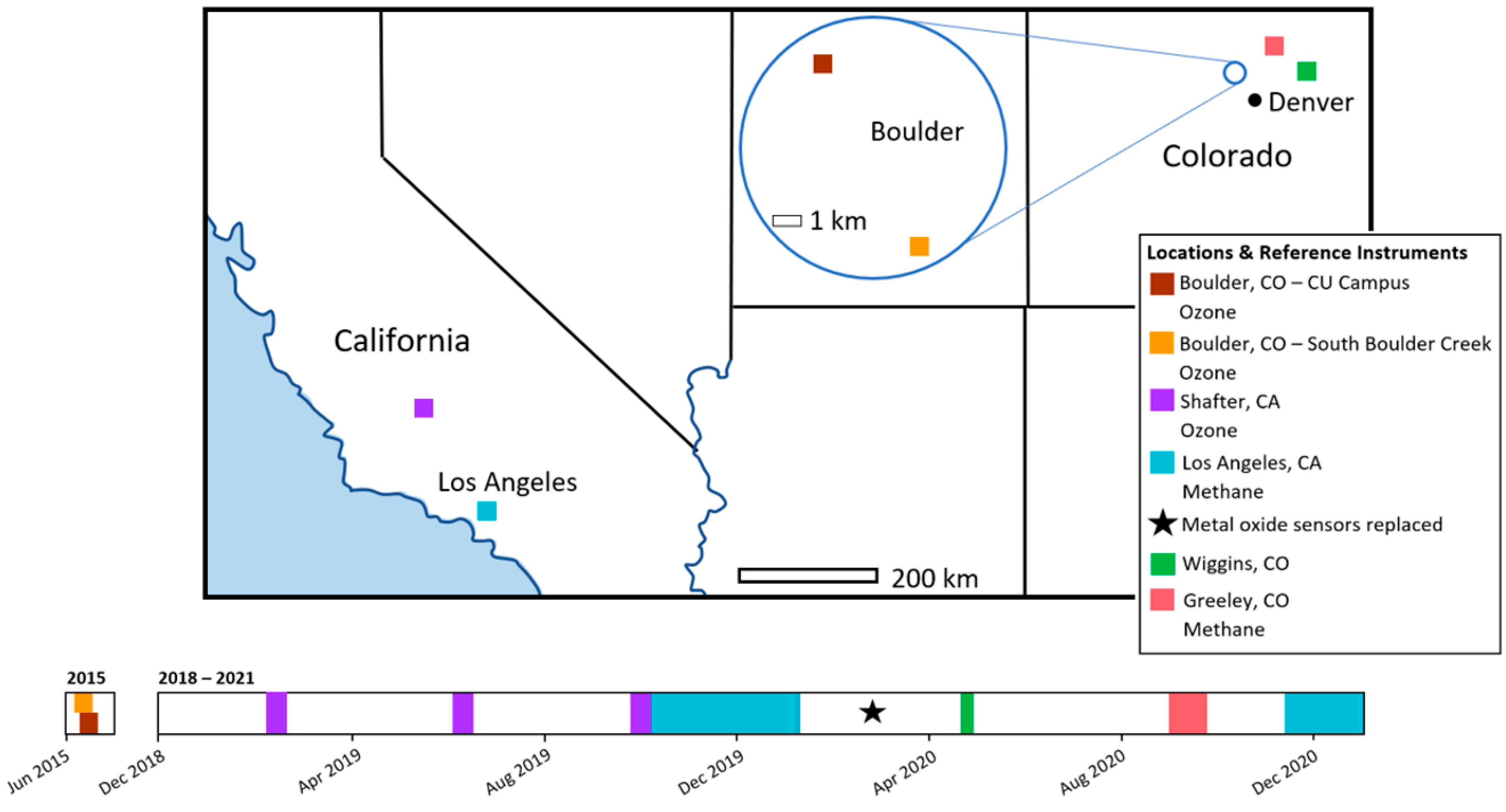
2.2. Sensor System Deployment Overview

Rather than distributing the sensors as a network, in this study, pods were stacked on top of each other or placed next to one another at each location to provide the most similar readings possible for comparing calibration techniques. In Los Angeles, the exact same location was used for calibration and validation, with different months of fall and winter being used for each. During the Colorado methane study, the calibration and validation spaces were approximately 60 km apart (Greeley and Wiggins, respectively). Both of these deployments had co-location periods lasting a month or longer in order to determine what conditions would produce the best calibration models. For the Colorado ozone study, however, we were only able to co-locate at the two reference locations for approximately a week each. Data collected at the South Boulder Creek site was used as calibration, while the pods located at the Boulder Campus site were used as validation. Note that this is also the only study that used two separate sets of pods for calibration and validation as we made use of data collected previously, rather than data collected with this particular study in mind as with the other co-locations.

2.3. Generalized Calibration Models

Regardless of the normalization approach, the same linear regression models were used to match the pod data to that of the reference instrument. Previous metal oxide sensor studies have shown the benefits of using temperature and humidity sensors to account for sensor sensitivities to environmental changes [1,2,3,4,5,10,13,14], as well as additional terms for each pollutant of interest. For methane, using both the heavy and light VOC sensors result in better calibrations [3,13]. Using an interaction term between the two VOC sensors [13], especially the ratio of light VOC signal to heavy VOC signal, has resulted in even better fits in a previous study [4]. For ozone, in addition to the inclusion of temperature and humidity sensors, previous studies have made use of a negative inverse temperature term to further improve fits [1,2,5]. The linear calibration models used for each pollutant of interest are listed in

Table 2. Linear Calibration Models.

Pollutant	Equation
Methane	CH4 (ppm) = p1 + p2*temperature + p3*humidity + p4*VOC1 + p5*VOC2 + p6*(VOC1/VOC2) + p7*elapsed time
Ozone	O3 (ppm) = p1 + p2*temperature +p3*1/temperature + p4*humidity + p5*o3 + p6*elapsed time

. In each equation, p represents the coefficients determined by the linear regression model, temperature is in Kelvin, humidity is absolute, and the metal oxide sensors are voltage in millivolts (mV).

Generally, the calibration-validation data splits were chosen due to data availability and intended purpose for each of the relevant analyses. For our initial test of all six calibration models, the 2019 Los Angeles data was split roughly in half into calibration and validation sets, with some slight seasonal change between the sets. The pair of Colorado deployments were used as calibration and validation, respectively. Finally, the Greeley data were used as calibration for the 2020–2021 Los Angeles validation data. A full description of how and why the data were split for each application can be found in Supplementary Table S2.

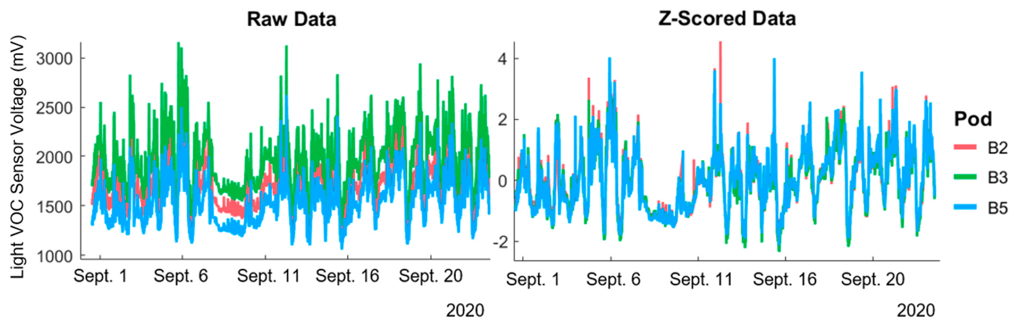
2.4. Sensor Signal Normalization Approaches

In the low-cost sensor world, either the voltage or calculated resistance of the metal oxide sensor has been used directly in calibration models, or a normalization has first been applied. We will focus on normalization techniques that ensure the signals among each pod are similar and therefore more transferable. The “individual” calibration model presented in Section 2.4 is the only one to utilize raw sensor signal data without normalizing it to the remainder of the pods first.

The rest of the normalization approaches studied here focus on transferability of data among pods. A sensor-specific normalization technique was utilized for methane by Collier-Oxandale et al., and will be revisited in this study as a comparison against the methods we develop here. For each of the raw signals used in the calibration model (temperature, humidity, light VOCs, heavy VOCs), a simple two-term linear regression was used to match the sensor signals of all but one of the pods to the remaining pod, which was selected to be used as a secondary standard [13]. These simple linear models are likewise applied to the raw signals for the validation data before proceeding with the overall model. This is the only approach we will explore that uses linear regression for the initial normalization process, and likewise the only approach that includes a separate normalization procedure matching individual sensors to their counterparts in another pod. Only one model in this work uses this approach, so we will refer to it as “sensor-specific normalization” for simplicity.

In this work, we attempt a z-scoring standardization approach. Each of the signals used from the pod was z-scored individually such that the mean of the sensor signal throughout the entire calibration period was subtracted out from each sample, and then divided out by the standard deviation over the same time frame. As a result, the new z-scored distributions of each sensor’s signals were centered to have a mean of zero and a standard deviation of one. Each sensor was z-scored individually; for example, one pod being used to quantify ozone would have three separate sets of z-scored data: one for the temperature sensor, one for humidity, and the ozone metal oxide sensor. If there were 1000 data points collected during the calibration period, we would use the z-score of each of those 1000 points in our models rather than using the raw voltages from the sensors. Signals from the reference instrument were not z-scored, and neither was the elapsed time imputed into each model. The remainder of the calibration models developed in this study utilize this approach. The specifications for each model are listed in

Table 3. Calibration Model Attributes, where X denotes a model having the selected attribute.

Model Attributes	Individual	Z-Scored Individual	Median	1-Cal	1-Hop	Sensor-Specific Normalization
All pods co-located at reference site	X	X	X
One pod co-located at reference site				X	X	X
Secondary co-location site					X	X
One quantification model			X	X		X
Quantification model for each pod	X	X			X
Quantification model for each sensor						X
Z-Score		X	X	X	X	X
Linear de-trending						X

.

Note that this method is different from the sensor-specific normalization in that each pod’s sensors are normalized with respect to themselves rather than attempting to match the signals to another pod. For instance, each individual ozone sensor reading is normalized based on its voltage relative to the voltage throughout the rest of the calibration period. Each sensor normalization is independent of all other sensors and pods.

We also explore log transform standardization in this work, applying it in a method like that used for z-scoring. The raw sensor signals from each pod were log transformed before applying each of the other sensor normalization or universal calibration models described in Table 1. In each case, model fits slightly worsened with the addition of this transformation. Even though the raw data exhibited diurnal trends and was approximately log normal, we hypothesize that transforming the data left it without enough variation to accurately capture the changes in concentration levels over time. Although this method was studied, we elected not to report the results in this work as this analysis proved to be worse than the other methods we have developed or improved.

2.5. Overview of Universal Calibration Models

In past field normalizations, linear regression has been used to fit the metal oxide, temperature, pressure, and humidity signals to that of a regulatory grade air quality monitor [1,2,3,4,5,10,13,14]. This approach requires every sensor-based instrument to be co-located with the reference instrument, and a unique set of model coefficients are generated for each sensor-based instrument (Figure 2a). In this study, we attempt universal calibration approaches, which only require one sensor-based instrument (for us, this is called a “pod”) to be co-located with the reference instrument, saving time and effort during the co-location stage of the process.

Since our pods are stationary, we focus on one-hop calibrations as opposed to multi-hop. Thus, only the one-hop calibration model includes a secondary co-location phase as our pods do not typically rendezvous in the field. Although calibration techniques other than linear regression have been proven to minimize error propagation over multiple hops, we do not take this into account since a simplistic, one-hop method best fits with stationary sensor platform deployment. Additionally, our version of a one-hop method only requires co-location with one reference instrument (one ground truth measurement) as opposed to more complicated schemes, which require frequent co-location with a reference instrument. It more realistic for research teams and citizen scientists that do not own a reference-grade instrument themselves and must seek access from a government facility to only have to do so once, rather than repeatedly, making it more accessible and applicable for small-scale projects.

2.5.1. Calibration Models Specific to Each Pod, Requiring Individual Co-Location

The individual approach (Figure 2a) is the simplest and most used calibration method, in which linear regression is used to create different calibration models for each pod. Every pod needs to be co-located with the reference instrument, and its models will have slightly different coefficients. In the z-scored individual model, we use this same physical setup, but opt to z-score the individual sensor signals to standardize the approach among pods.

2.5.2. Multi-Pod Calibration Models, Requiring One Pod to Be Co-Located with a Reference

In this work, we pilot a new multi-pod calibration approach, which we dub one-cal. After co-locating just one pod with the reference instrument, the pod sensor signals are z-scored, and a linear regression model is developed using this z-scored data only. For the remainder of the pods that were not co-located, their sensor signals are likewise z-scored, and the previously developed linear regression model is applied according to the physical setup in Figure 2b.

An already established multi-pod calibration model known as one-hop was also applied to our data in combination with our z-score standardization approach. For this approach, one pod was similarly co-located, all sensors z-scored, and a linear regression model was generated. In a secondary calibration step, the reference co-located pod is now treated as the reference instrument, and is co-located with the remainder of the pods. The reference co-located pod is often referred to as the secondary standard. The sensor signals of the remaining pods are then z-scored, and linear regressions are developed to match the z-scored signals of these additional pods to the secondary standard pod, as shown in the physical setup in Figure 2c.

An additional multi-pod calibration approach required the physical setup shown in Figure 2a, where all pods are co-located with the reference instrument. The signals of each pod are then z-scored, and the median z-score at each timestamp across all pods is chosen as the dataset to generate a calibration model on. This model is then applied to the z-scored signals of each of the pods. Figure 3 shows the increased uniformity of the z-scored pod signals, making the z-scoring signal standardization approach more transferable among pods.

The sensor-specific normalization process created by Collier-Oxandale et al. and revisited here also only requires one pod to be co-located with a reference instrument, although it is more involved than the other two methods listed here in that each pod requires multiple rounds of normalization. After the one co-located pod is co-located with the remainder of the pods, the raw signals of each sensor from the remaining pods are matched to the raw sensor signals of the pod that was co-located using a two-term linear regression model. Then, the linear regression model matching the co-located pod to the reference instrument is applied to each of the remaining pods. Even though only one pod is co-located in this process and one overarching calibration model is applied, the three or four two-term regressions required for each pod add complexity to the process overall.

While the sensor-specific normalization and one-hop calibration approaches require two separate co-location periods (Figure 2c), additional datasets of non-spatially dispersed pods were not available to us. Thus, we used data where all pods were co-located with the reference instrument as both a single pod reference calibration as well as a pod-to-pod calibration; we proceeded as if only one pod was located there during the first step, and then as if the reference instrument was not there during the second step. Since both calibration steps took place in the same location at the same time, it is possible that our results for these two approaches might be biased high in terms of model fits, since using two separate physical spaces and time periods would likely introduce more variability into all the sensor signals. While we do not expect that this would have affected fits dramatically, it is important to note that to use the same dataset as all the other models, we did not experience the benefits of only having to co-locate one pod with a reference instrument throughout these experiments.

2.6. Calibration Model Evaluation

To evaluate the quantification scheme performance, we rely on three main statistics: coefficient of determination (R²), centered root mean square difference (CRMSD), and centered mean bias error (cMBE, referred to in this work as MBE). Note that the CRMSD and MBE are normalized values and have been shown to be useful when evaluating models using quantification target plots [15]. The formulas used to determine each are listed below in

Table 4. Selected Statistics and Relevant Formulas.

Statistic	Formula	Relevant Terms
R2	$1-\frac{SSE}{TSS}$	SSE = sum of squared errors TSS = total sum of squares
CRMSE	$\sqrt{{{\displaystyle \sum }}^{ }\frac{n^N{\left[\left(p-\overline{p}\right)\left(r-\overline{r}\right)\right]}^2}{N}}$	N = total number of samples n = current sample p = concentration predicted using model
MBE	$\overline{p}-\overline{r}$	r = concentration from reference instrument

[30]. In our analysis, we will refer to R² as the correlation between a pod and the reference instrument, the CRMSE as the random error, and the MBE as the bias. Since only calibration and validation data were used in our analyses, data cleaning was minimal. All data was minutely averaged (one measurement per minute) unless otherwise stated, and minimal data smoothing and spike removal were utilized to ensure reasonable results.

3. Results

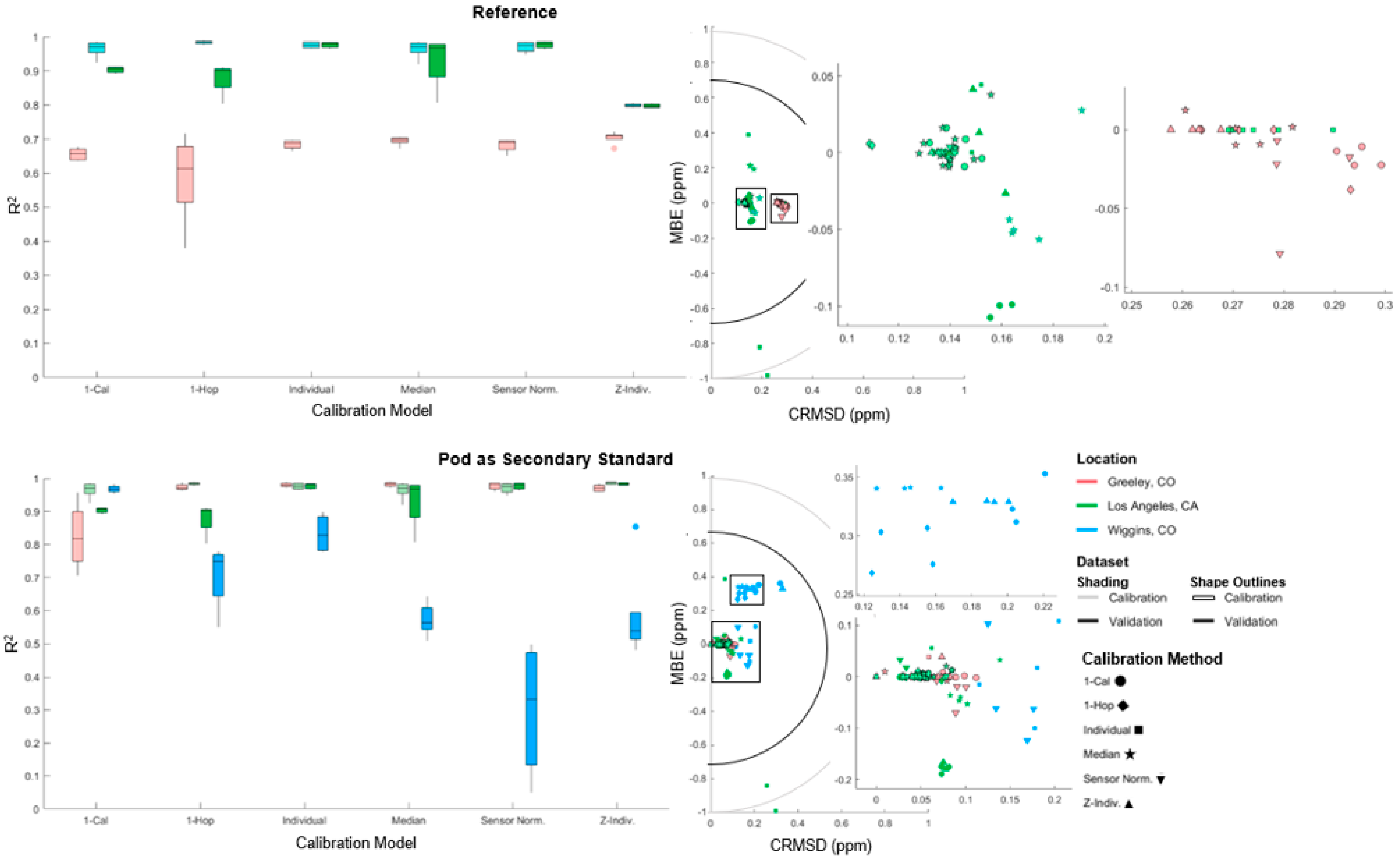
3.1. Applying Universal Calibration Models

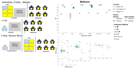
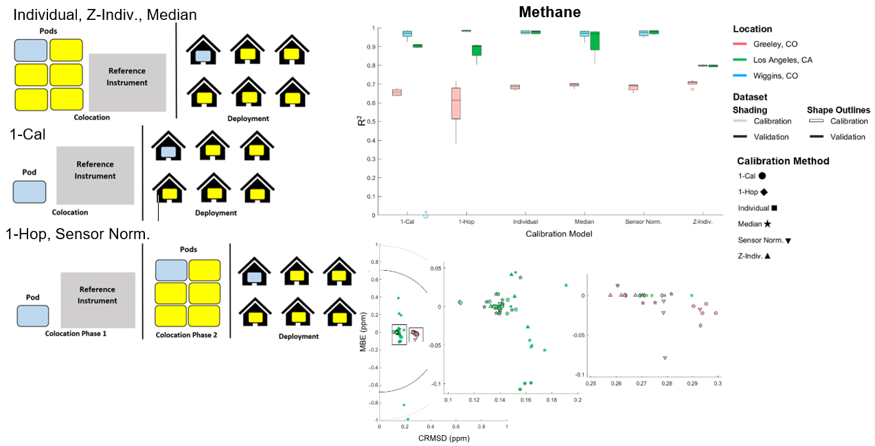
3.1.1. Methane Results

For studies where methane concentration is being measured, a slight decrease in accuracy and precision as assessed with goodness of fit statistics might be viewed as worthwhile if the ease of implementing that sensor quantification scheme is significantly reduced.

Here, the 1-Cal and 1-Hop quantification approaches each result in simplified quantification models as well as reduced time and energy for co-location. In Figure 4, we show the selected statistics for each calibration approach for the three deployments mentioned above (Los Angeles—calibration and validation, Greeley—calibration, and Wiggins—validation). These model performance statistics are also listed for each approach used in the supplemental (Supplementary Tables S3 and S4). The variation in the boxplots and the repeating points on the target plots represent the metrics for each individual pod, namely four in Los Angeles, and six in each Colorado location. At the Wiggins co-location site, a reference monitor was not available. Thus, we have included two different sets of statistics: one comparing the pod fits against reference instruments, where available, and another comparing pod fits against a pod that was co-located as a secondary standard.

From these results, the 1-Cal approach yields a reasonable trade-off between correlation, error, and bias. Calibration outcomes in the warm environment at sea level in Los Angeles, California mirrored those at high altitude in Boulder, Colorado, indicating that the method is successful so long as a similar range of sensor readings are reflected in the calibration and validation phases. Although the comparisons against the individually calibrated pod are undoubtedly less accurate than those with a regulatory-grade instrument, the same trends hold for both locations, further proving the utility of the 1-Cal method in the absence of a better reference in Wiggins. In Los Angeles, calibration and validation data were collected at the same location months apart, while in Colorado, the datasets were separated by approximately 60 km as well as a few months. The difference in location explains the worse validation fits in Colorado, since fitting and deploying on identical temperature and humidity spaces with the same range of pollutant concentrations makes the data more transferrable. The most obvious split of fits in the target plot of Figure 4 is between pods co-located in different environments. This is discussed in Section 4.3. The metrics included using a pod as a secondary standard show how closely a pod can imitate another pod even if there is more deviation from the reference instrument; errors do not seem to exhibit much additional propagation when translating from one pod to another. In lieu of reference data at the Wiggins site, the statistics calculated between each pod and the individually calibrated pod treated as a secondary standard still show the relative goodness of fit across different calibration models.

Beyond the clustering of different locations on the target plots, we notice that the points corresponding to specific normalization or calibration approaches are also generally clustered, with a few exceptions and patterns emerging. For the 1-Cal model, the Los Angeles co-location data shows that even as the CRMSD increases, the bias remains centered nearly at zero, demonstrating that bias is less significant for this specific application. However, the Greeley calibration data and Los Angeles validation data show more mixed results with both bias and CRMSD changing among pods, making it more difficult to come to concrete conclusions about the models’ ability to minimize errors. Interestingly, the individual models (“individual”, “z-indiv.”) show the most outliers outside of the two major clusters of points, suggesting that the standardization and multi-pod calibration approaches do their part to minimize error and make results more consistent across pods. Since the raw signals of individual pods are often similar for the majority with a few outliers, these outlying pods can be seen in the clusters that formed for the median model on the target plot. Errors for some pods may have been driven higher by their signals not being chosen as the median during model generation, placing some, but not all, median model pods in a statistical middle ground.

3.1.2. Ozone Results

Data collected in 2015 in Boulder, CO, USA was utilized to see how well the calibration models performed in another environment. Since this data was collected in years prior, it was not optimized for this exact use and thus performed worse than methane generally. As further discussed in Section 3.4, we recommend co-locating sensors with a reference instrument approximately two weeks to successfully field normalize using the universal calibration approach. In Boulder, only nine days of co-location data were available, resulting in worse fits than we would anticipate if designing an experiment specifically for the implementation of a universal calibration model. Additionally, the co-location and validation data represent two different sets of pods. No pod was both calibrated and validated, but rather the calibrations generated on one set were applied to a unique set of pods as validation. Thus, the 1-Hop and Sensor signal normalization approaches, which require the “main” pod co-located with the reference instrument to then be co-located with the remainder of the pods, were not utilized.

Aside from the issues stemming from the experimental setup, the R² results for ozone in both locations (Figure 5) mirror those observed for methane. Reference monitors were available at each co-location site, so measures of fit are all relative to the reference instruments rather than individual pods. Interestingly, most points on the target plot form a cross; models generally either suffered from random error or bias, but not both. The 1-Cal and Sensor signal normalization struggled more with bias, the Median results were not consistent, and the other models experienced random error but less bias. While there was still some clustering based on location, it was less obvious for ozone than for methane, perhaps because neither the California nor the Colorado data had been collected with this end-use in mind; the shortcomings of each were more similar. Given the experimental constraints, the 1-Cal approach still appears to be a viable option for co-locating just one pod with a reference instrument rather than the entire fleet, although given the increased bias might not be as suggestive as it is for methane. However, the viability of the standardization and multi-pod calibration models are demonstrated by the consistent measures of fit for ozone, although different patterns were observed on a smaller scale.

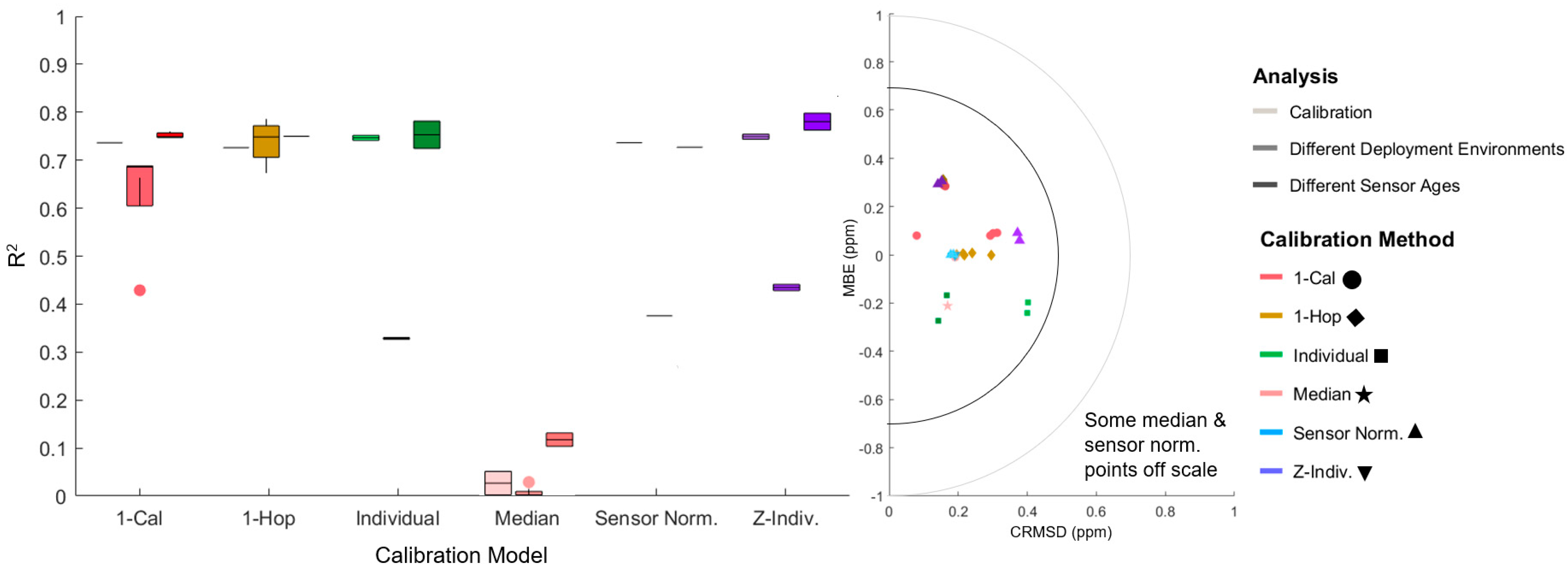
3.2. Ability of Universal Calibration to Correct otherIissues Plaguing Low-Cost Sensors

3.2.1. Co-Locating and Deploying Sensors in Different Environments

Ordinarily, pods need to be co-located and deployed in similar environments due to the significant influence of temperature, humidity, and pressure on sensor readings. In this portion of the analysis, we apply each of our calibration models from Los Angeles, CA, USA and apply them to the data collected in Greeley, CO, USA. Note that the Los Angeles data was collected from November 2020 to January 2021 at the same location as the previous Los Angeles co-location. The sensors in each of the pods were replaced with new ones just prior to the Colorado deployments in 2020, so data reflecting the new sensors were required to account for differences between the new sensors and ones that had already been in use for a few years during the previous Los Angeles collection.

In Figure 6, we see that the individual model may have struggled to translate from the warm environment at sea level in Los Angeles to the higher altitude in Colorado. The median model also fits particularly poorly, likely due to a lack of available co-location data. Only two pods were available for this additional co-location in Los Angeles, resulting in a less-than representative sample of pod data that struggled to capture both the different environment in Colorado as well as the four additional pods that data was not drawn from. The two additional universal calibration methods, however, performed reasonably well, especially the 1-Hop method. We hypothesize that by using the z-score standardization of all the sensor signals, especially the temperature and humidity, increased uniformity, making the calibration more transferable. Rather than attempting to fit vastly different temperature and humidity spaces, fitting on scaled-down versions of the same data makes the process much less dependent on the actual temperature and humidity spreads. On the target plot, calibration schemes with multiple pods saw those pods clustered together, but there were noticeable differences in bias and random error among different methods.

While co-locating in the same environment as deploying is still recommended, the use of the 1-Hop method can be a viable alternative when a reference instrument is not available in areas of interest. This greatly widens the ability to deploy sensors in areas that were previously avoided due to the lack of suitable reference instruments, all while still providing the benefits of universal calibration in terms of time and effort. The physical co-location and deployment schemes as well as the normalization approach are large factors in the transferability of data, but the z-score standardization approach is promising for scenarios when the physical setup is not optimal.

3.2.2. Age of Sensors

In past deployments, the age of the metal oxide sensors has been associated with data quality and model transferability. The sensor-specific normalization process developed by Collier-Oxandale et al. [13] and further studied here includes a detrending process thought to account for the sensors being different ages, which may result in differences in drift and the noise associated with signals [4]. In a multi-year study in Los Angeles, we noted that metal oxide sensor signals became noisier and less reliable after approximately three years of use in the field, recommending that the sensors be replaced after two years of use [4]. In a laboratory setting, the metal oxide sensors have shown noticeable drift in under a year [31]. To better understand how sensor age affects calibration fit, we collected an additional set of data at the Los Angeles site from late 2020 to early 2021, and applied calibration models generated here to the late 2019 set of Los Angeles methane data previously studied in this work. Note that the metal oxide sensors were replaced in the spring of 2020, making them about eight months old at the time of the most recent study. During the previous 2019–2020 deployment, the sensors were approximately three and a half years old.

The fits associated with applying the 2020–2021 models to the 2019 data are shown in Figure 6. Specifically, note the darkest shaded markers. The z-score standardization models (1-Cal, 1-Hop, Z-Indiv.) fit the best overall, suggesting that normalizing the data first can account for any increased noise experienced over time in the sensors. Of these, the 1-Hop demonstrated the most consistently low biases and random errors among each of its pods, with 1-Cal as close runner up. The Z-Indiv. experienced the most bias out of the three. Surprisingly, the individual calibration models fit similarly to the standardized models, despite exhibiting a wider range of fits. Small raw signal bias between co-located sensors (see Figure 3) has historically been attributed to differences in the sensors themselves, but the relative ease of transferability among replaced sensors even for non-standardized signals suggests that the differences observed among pods is likely attributed to the individual printed circuit boards (PCBs) rather than the sensors themselves, as the effectiveness of the copper traces may also vary by board with time.

Note that only two pods were re-co-located at the Los Angeles site in late 2020. Thus, for the models that require a pod-specific calibration (Individual, 1-Hop, Sensor Norm), the boxplots only reflect two pods, while those that apply the same model to every pod reflect the fits of all four pods available (Median, 1-Cal). This may be part of why the median model performed the worst for this application; the two available pods may not have been the most representative of the data, and differences among the two may have contributed to a slightly disjointed model. Rather than being railing-mounted or stacked on top of a container, as in all previous co-locations, the pods had to be stacked directly on the roof of the trailer for the 2020–2021 co-location due to physical constraints. Thus, the pod on the bottom of the stack may have had reduced airflow, which could have skewed the medians used in the model, resulting in worse fits. Throughout each of these analyses, the Median model has been one of the least robust in general and does not save time or effort as all pods still need to be co-located to implement it.

3.3. Factors Affecting Individual Calibration

3.3.1. Duration of Co-Location

When co-locating low-cost sensors, we encounter tradeoffs between simplicity and accuracy and sometimes struggle with resource needs. Since the regulatory-grade instruments are primarily employed to meet the regulatory framework, sensor system co-locations are often subject to suboptimal timelines and availability. Here, with long-term access to multiple reference instruments, we explore what co-location conditions are optimal so we can request the exact length of time and reference instruments in the future that will yield the best calibration results. Two different methane reference instruments were available at the co-location site in Los Angeles. The measures of fit of all the individually calibrated pods compared to each reference instrument is presented in Figure 7. Calibration and validation were randomly selected from the same six-week period when the two available reference instruments demonstrated the highest degree of data completeness and similarity. A three-fold algorithm was used for the randomized data selection. Validation 2 represents an earlier month of data in the same location (see Supplementary Table S2).

Although the shortest amount of time (one week) yielded the best calibration R² values regardless of the reference instrument for both the calibration and validation data, this is likely due to overfitting and would not necessarily translate the best to deployment data, for which we want to capture the largest range of sensor signals possible so as not to extrapolate. The validation data demonstrates this; the more calibration data used, the higher the correlations and the smaller the variability in fits. The target plot further exaggerates the differences between the calibration and validation data fits. All the calibration data is clustered near the origin, experiencing the smallest random error and bias alike. The validation data, however, is arranged in a nearly vertical line, demonstrating how random error is relatively constant regardless of the duration of co-location, but how bias changes across time. Longer calibration periods produced fits that were biased low, while shorter to more moderate calibration periods yielded data biased high. This might have been caused by small baseline shifts experienced by the reference instruments’ calibration during the co-location period.

3.3.2. Reference Instrument Calibrations

Two methane reference instruments developed by two different manufacturers, Picarro and Thermo, were available at the reference site in Los Angeles. The specifications of each can be found in the supplemental (Supplementary Table S1). For our analysis, we selected a six-week period that had the most data completeness for both analyzers. For instance, the Thermo experienced calibration issues early on, and then did not log for a few days while repairs and recalibration took place. We focused on later data to avoid these calibration issues confounding our results, as shown in Figure 8. In general, the Picarro instrument yielded concentrations that resulted in model fit statistics that were slightly better than the Thermo, likely due to small differences in calibration techniques (Figure 7). For the selected period, the two instruments had an R² of 0.97, and an RMSE of 0.07 ppm between them. Generally, avoiding periods of atypical spikes and data loss improved our calibration fits, although during most co-locations these may be unavoidable since the reference data cannot be analyzed until the end. If possible, we recommend co-locating for longer periods of time than required so that additional periods of data are available in the event of a power loss, calibration issue, or unusual air quality event. The target plot trends for each reference instrument mirrored each other; for the calibration data, a small shift in bias is the only noteworthy difference from the otherwise identical points, and both experienced the same issues with validation described in Section 3.3.1.

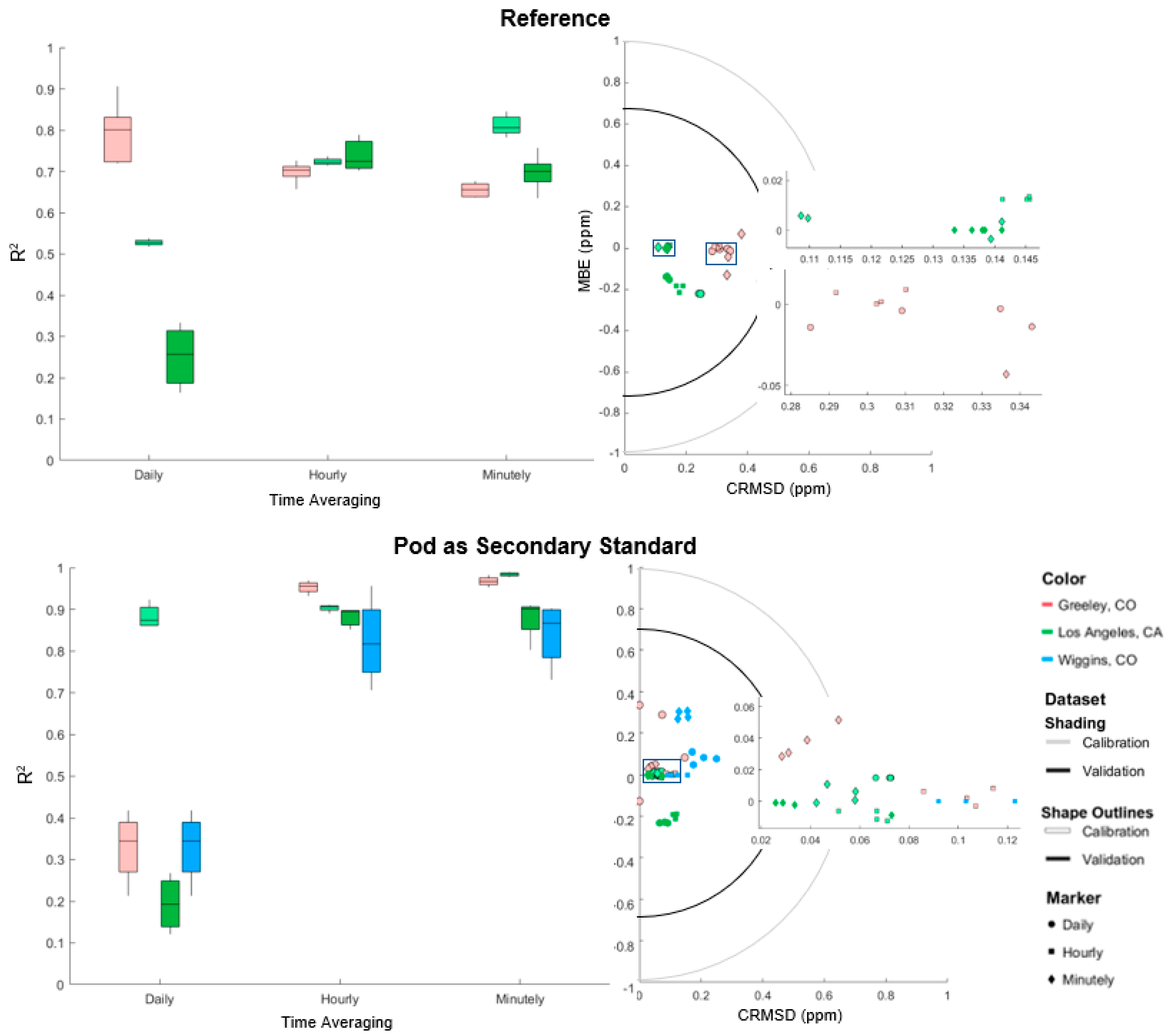
3.4. Factors Affecting Universal Calibration

3.4.1. Duration of Co-Location

For the first universal calibration approach, in which one model is generated and applied to all pods, the co-location process for that one pod occurs the most similarly to the individual calibration process. Since only one model is being generated, the same time length of co-location is recommended for this approach. For the second universal calibration method, which requires two distinct co-location phases, the time requirements will vary. The first step of the co-location process with one pod and the reference instrument should be carried out the same as for an individual pod and the first type of universal calibration. For the co-location between the secondary standard pod and the remainder of the pods, however, a separate analysis was conducted to determine the appropriate duration of “hop”. We will focus on methane in this section since ozone reference data was only available in one week increments for the Colorado deployment.

As shown in Figure 9, the results for this analysis were more mixed for the two different locations. In Los Angeles, the length of co-location between the pod being used as a secondary standard and the remainder of the pods informed the calibration fits to a great extent. The longer this secondary co-location, or “hop”, lasted, the better the models performed for the remainder of the pods. In Los Angeles, a minimum of two weeks is recommended to maximize correlation and minimize uncertainty using the 1-Hop method.

While the Los Angeles dataset showed a clear correlation between length of time and calibration fits, the goodness of fits of the Colorado data remained relatively constant regardless of how long the secondary co-location lasted. The only true differences are seen in the validation dataset, which similarly prove that using two weeks or more of co-location can improve fits dramatically. For the Colorado validation data, since there was no reference instrument available in Wiggins, the trends are harder to interpret. These measures of fit were calculated using one normalized pod as a secondary standard for each dataset to have a fair comparison. Since the calibration pods match the secondary standard pod so closely, the trends seen against the reference instrument become less obvious. For the Los Angeles dataset, the differences in the calibration fits become almost non-existent, while the validation improvements with time remain obvious. This may have to do with error propagation along hops that many groups have set out to minimize. Even though the calibration data does not appear significantly better or worse, the importance of the longer co-location is still evident in the validation data.

We observe similar trends in the Colorado calibration data, but the opposite for our validation data. Validation fits are comparatively more constant but experience small decreases in goodness of fit as co-location time increases. Fits were also biased low in an almost linear fashion. There are a few possible reasons for this disparity. Firstly, the Los Angeles calibration and validation datasets were in the exact same location, so any error associated with different environmental conditions in different locations would be nonexistent. With the calibration and validation co-location areas in Colorado were approximately 60 km apart, there is more room for error as the model may have fit on slightly different environmental parameters such as temperature and humidity between the two locations. We discuss the differences in concentrations and environmental parameters among locations further in Section 4.3. While this is the most likely explanation, it is also possible that the vastly different environmental conditions between urban Los Angeles and suburban-to-rural Colorado, including the absolute pressures at two very different altitudes, may have contributed to a lack of transferability between the two locations. However, without the possibility of comparison with a reference instrument in the Greeley, Colorado location, it is harder to determine how well the validation data performed, since error likely propagated in the secondary standard pod.

3.4.2. Time Averaging

We also explored the effects of different time averaging with the 1-Hop method to determine at what resolution reference data would be needed to produce adequate results. The calibration and validation results are shown in Figure 10 for methane. For some of the calibration data, lower resolutions result in better fits, although this is likely due to overfitting with fewer data points available. However, for the validation data, hourly averaged data or a higher resolution is necessary for this method to be effective. This is likely due to the smaller range of sensor and environmental signals experienced with increased time averaging. Within the target plot groupings based on location, the Los Angeles data is most in line with expectations; the minutely data lies closest to the origin with the most minimal fluctuations in bias and random error, while hourly and then daily experienced more error, but were not far off. The Greeley data, however, appears to be the opposite, with minutely data experiencing more bias and random error than the other time averaging approaches. It is worth noting that the Greeley co-location was slightly shorter than the one in Los Angeles, so having fewer data points available for the daily and even hourly schemes may have contributed to overfitting in individual models. The Greeley dataset’s matching validation data in Wiggins reinforces that overfitting was a major issue. Although fits look different when using a pod as a secondary standard in lieu of a reference instrument at this location, the calibration overfitting is obvious, with minutely time averaging performing best.

4. Discussion

4.1. Benefits of Standardizing Sensor Data

One of the major takeaways from utilizing a universal calibration method was the added precision of z-score standardization of each of the sensor signals. Since the sensors used are all inexpensive, they are not particularly accurate, and sensors deployed in the same exact location will still have differences in their numeric output. By switching to the z-score, we eliminated the bias between pods, resulting in an almost completely uniform sensor timeseries across all pods. This made our universal calibration efforts much more reproducible, even in vastly different physical environments and in sensors of varying ages. The main shortcoming may include less reliability in field data applications where elevated baselines are present, as discussed further in Section 4.4. Each of the signal normalization approaches studied in this work demonstrate an important step in the path from individual to multi-pod and even universal calibration model schemes.

4.2. Using a Field Normalized Pod as a Secondary Standard

At the location where a reference-grade monitor was not available, we used a field normalized pod as a secondary standard to quantify our results. Due to the inherent random error between the reference and the pod and the similarity among pods after the z-score standardization process, the model fit statistics for a pod (when compared to the secondary standard) appear much better than they actually are. While this approach to data validation is not ideal for this reason, the general trends in goodness of fit hold up regardless of the method used. To obtain a value closer to what the reference would have provided, the goodness of fit value calculated against the reference instrument can be divided by the goodness of fit value between the secondary standard pod and the actual reference instrument. While this is not a perfect approximation, in our study, this calculated value was less than 2% off from the actual reference-tabulated value for methane. While a regulatory-grade reference instrument is still preferred, the predictability and repeatability of these results make the pod as a secondary standard method more reliable and trustworthy for when a better reference is not available.

4.3. Influence of Location on Pod Fits

Regardless of the calibration or normalization approach used, model fit statistics tended to be better in some locations as opposed to others. For methane, model fit statistics were consistently better in Los Angeles than in Colorado. The range of concentrations as well as the environmental variability was generally smaller in California than in Colorado, making it easier for any singular model to fit the data. Co-location standard deviations from the reference instruments (LA = ±0.297 ppm, CO = ±0.537 ppm) as well as the temperature standard deviations, since the metal oxide sensors are sensitive to fluctuations in temperature (LA = ±4.75 K, CO = ±11.70 K) were larger in Colorado. The more consistent concentrations and environment in Los Angeles meant less variability for any singular model to attempt to capture, and thus better calibration fits. Furthermore, by moving the monitors to another location for validation in Colorado during a different season, even more variability was introduced, while calibrating and validation sensors in the same exact location in California kept the ranges of concentrations and temperatures more consistent, and easier for the models to replicate.

Aside from the variability, the proximity to oil and gas activity and differing oilfields may have contributed to the observed differences in calibration fits for methane. While each co-location site was in the vicinity of oil and gas operations, both sites in Colorado were markedly closer to active oil wells, and may have experienced more episodic spikes, which can be harder for models to capture. A portion of the Los Angeles reference data was only available as five-minute average rather than minutely, which may have contributed to better fits in this area. However, the remainder of the data was minutely averaged and was recorded for nearly the same amount of time at each site. The physical setup of pods at each co-location site was nearly identical, as a further control among studies.

For ozone, the differences in model fit statistics among the three locations studied also boils down to variability, but may have more to do with time of year and environmental factors than location. In Colorado, the calibration and validation sites were located mere kilometers apart, and data was collected during the same month, so environmental variability between the two was generally low. In California, although the same location was used for calibration and validation, the data spanned three weeks across seven months, introducing considerably more seasonal variability. Calibration data from both winter and summer were used to fit spring validation data. Although this “bookending” approach has been used to calibrate metal oxide sensors when better data is not available [4], the two different seasons had markedly different concentration standard deviations (winter = 13.01 ppb, summer = 20.49 ppb) and reasonably different temperature (winter = 5.14 K, summer = 8.99 K) standard deviations. Interestingly, the humidity space appears to be less important, exhibiting less variability and therefore less influence on the models. While this demonstrates that the models studied are appropriate in different concentration, temperature, and humidity spaces, we believe the inconsistencies among locations are due to these external differences rather than shortcomings of the models themselves. Too much variability is generally detrimental to metal oxide sensors regardless of the approach used.

4.4. Co-Location Recommendations

Since the individual, z-scored individual, and median models require every pod to be co-located with a reference instrument, they are more cumbersome physically despite the reliable fits of the individual model when co-locating and deploying in the same physical environment. As we have explored here, there are many reasons to shift to a multi-pod calibration approach, from reducing the burden of co-locating a full fleet of sensors to more reliability deploying in different environments or using sensors of different ages. While recommendations will vary depending on the goals and physical restrictions of an individual study, we have found that normalizing sensor signals using their z-score is a reliable method for making low-cost sensor data more transferrable among units. While the 1-Hop method is generally reliable, it does require at least two weeks of a secondary co-location among the individually calibrated pod and the rest of the fleet. In balancing the ease of physical setup and reliability of results, the 1-Cal checks most boxes as a fair tradeoff among methods.

4.5. Considerations for Field Applications

In this work, we have focused exclusively on field normalization techniques for co-located pods. While additional datasets serving as validation data effectively behaved as field data, the pods were still placed in the same location, with sensor signals that should be nearly identical to begin with. When pods are spatially distributed in the field, we expect to observe more variation. When using z-score standardization models, the pod sensor signals are centered around zero, unlike the raw voltage, which is typically in the hundreds for temperature in Kelvin, or the thousands of mV for metal oxide sensor signals. Due to the huge difference in scale between z-scored and raw pod data, the field data also needs to be z-scored if this approach is used so that the ppm-converted results will be the correct magnitude.

While this did not pose any major issues for the data studied in this work, we believe that this approach could cause field-deployed pods with elevated concentrations to be biased low, with a higher baseline still being centered at zero in the z-scored pod data. Since these effects have not been extensively studied yet, it is recommended that this method be used more for areas where significant baseline shifts will not be observed, focusing more on concentration spikes, which will be more adequately translated by this method.

4.6. Broader Implications

Since these calibration methods show similar results for both methane and ozone, they appear to be effective in calibrating metal oxide sensors regardless of the target gas, allowing for applications in other gases. Additionally, the reproducibility of results achieved using a z-score standardization approach vastly improve model fit statistics for pods calibrated in one environment and deployed in another, suggesting that low-cost sensor studies could now take place in areas without ample access to reference-grade monitors. Thus, the expansion of sensor normalization techniques and multi-pod or universal models for calibrating entire fleets of low-cost sensors could make their use easier and more geographically widespread.

5. Conclusions

Although individual calibration models still perform better than multi-pod or universal models when calibrated and deployed in a similar environment, sensor normalization techniques make single-pod calibration schemes more feasible and reliable. The z-score standardization approach specifically has great potential among sensors of varying ages and those deployed in different environments alike. While this method has not been tested for mobile sensors, which are prone to error propagation across multiple hops, the 1-Cal approach avoids error propagation all together by using a single calibration model. The 1-Cal method is only outperformed by the more widely used 1-Hop method when calibrating and deploying sensors in vastly different environmental spaces. Large extrapolations are still not recommended, but by designing experimental setups with the 1-Cal or 1-Hop in mind, easy and reliable calibration results can be achieved.

References

1. Collier-Oxandale, A.; Coffey, E.; Thorson, J.; Johnston, J.; Hannigan, M. Comparing Building and Neighborhood-Scale Variability of CO2 and O3 to Inform Deployment Considerations for Low-Cost Sensor System Use. Sensors 2018, 18, 1349. [Google Scholar] [CrossRef] [Green Version]
2. Cheadle, L.; Deanes, L.; Sadighi, K.; Gordon Casey, J.; Collier-Oxandale, A.; Hannigan, M. Quantifying Neighborhood-Scale Spatial Variations of Ozone at Open Space and Urban Sites in Boulder, Colorado Using Low-Cost Sensor Technology. Sensors 2017, 17, 2072. [Google Scholar] [CrossRef] [Green Version]
3. Collier-Oxandale, A.; Wong, N.; Navarro, S.; Johnston, J.; Hannigan, M. Using gas-phase air quality sensors to disentangle potential sources in a Los Angeles neighborhood. Atmos. Environ. 2020, 233. [Google Scholar] [CrossRef]
4. Okorn, K.; Jimenez, A.; Collier-Oxandale, A.; Johnston, J.; Hannigan, M. Characterizing methane and total non-methane hydrocarbon levels in Los Angeles communities with oil and gas facilities using air quality monitors. Sci. Total Environ. 2021, 146194. [Google Scholar] [CrossRef]
5. Sadighi, K.; Coffey, E.; Polidori, A.; Feenstra, B.; Lv, Q.; Henze, D.K.; Hannigan, M. Intra-urban spatial variability of surface ozone in Riverside, CA: Viability and validation of low-cost sensors. Atmos. Meas. Tech. 2018, 11, 1777–1792. [Google Scholar] [CrossRef] [Green Version]
6. Ripoll, A.; Viana, M.; Padrosa, M.; Querol, X.; Minutolo, A.; Hou, K.M.; Barcelo-Ordinas, J.M.; Garcia-Vidal, J. Testing the performance of sensors for ozone pollution monitoring in a citizen science approach. Sci. Total Environ. 2019, 651, 116–1179. [Google Scholar] [CrossRef]
7. Spinelle, L.; Gerboles, M.; Villani, M.G.; Aleixandre, M.; Bonavitacola, F. Field calibration of a cluster of low-cost available sensors for air quality monitoring. Part A: Ozone and nitrogen dioxide. Sens. Actuators B Chem. 2015, 215, 249–257. [Google Scholar] [CrossRef]
8. Suriano, D.; Cassano, G.; Penza, M. Design and Development of a Flexible, Plug-and-Play, Cost-Effective Tool for on-Field Evaluation of Gas Sensors. J. Sens. 2020, 2020. [Google Scholar] [CrossRef]
9. Sayahi, T.; Garff, A.; Quah, T.; Lê, K.; Becnel, T.; Powell, K.M.; Gaillardon, P.E.; Butterfield, A.E.; Kelly, K.E. Long-term calibration models to estimate ozone concentrations with a metal oxide sensor. Environ. Pollut. 2020, 267, 115363. [Google Scholar] [CrossRef]
10. Casey, J.; Collier-Oxandale, A.; Hannigan, M. Performance of artificial neural networks and linear models to quantify 4 trace gas species in an oil and gas production region with low-cost sensors. Sens. Actuators B Chem. 2019, 283, 504–514. [Google Scholar] [CrossRef]
11. Honeycutt, W.T.; Ley, M.T.; Materer, N.F. Precision and Limits of Detection for Selected Commercially Available, Low-Cost Carbon Dioxide and Methane Gas Sensors. Sensors 2018, 19, 3157. [Google Scholar] [CrossRef] [PubMed] [Green Version]
12. Zaidan, M.A.; Motlagh, N.H.; Fung, P.L.; Lu, D.; Timonen, H.; Kuula, J.; Niemi, J.V.; Tarkoma, S.; Petäjä, T.; Kulmala, M.; et al. Intelligent Calibration and Virtual Sensing for Integrated Low-Cost Air Quality Sensors. IEEE Sens. J. 2020, 20, 13638–13652. [Google Scholar] [CrossRef]
13. Collier-Oxandale, A.; Casey, J.G.; Piedrahita, R.; Ortega, J.; Halliday, H.; Johnston, J.; Hannigan, M. Assessing a low-cost methane sensor quantification system for use in complex rural and urban environments. Atmos. Meas. Tech. 2018, 11, 3569–3594. [Google Scholar] [CrossRef] [PubMed] [Green Version]
14. Piedrahita, R.; Xiang, Y.; Masson, N.; Ortega, J.; Collier, A.; Jiang, Y.; Li, K.; Dick, R.P.; Lv, Q.; Hannigan, M.; et al. The next generation of low-cost personal air quality sensors for quantitative exposure monitoring. Atmos. Meas. Tech. 2014, 7, 3325–3336. [Google Scholar] [CrossRef] [Green Version]
15. Casey, J.G.; Hannigan, M. Testing the performance of field calibration techniques for low-cost gas sensors in new deployment locations: Across a county line and across Colorado. Atmos. Meas. Tech. 2018, 11, 6351–6378. [Google Scholar] [CrossRef] [Green Version]
16. Maag, B.; Zhou, Z.; Thiele, L. Enhancing Multi-Hop Sensor Calibration with Uncertainty Estimates. In Proceedings of the 2019 IEEE SmartWorld, Ubiquitous Intelligence & Computing, Advanced & Trusted Computing, Scalable Computing & Communications, Cloud & Big Data Computing, Internet of People and Smart City Innovation (SmartWorld/SCALCOM/UIC/ATC/CBDCom/IOP/SCI), Leicester, UK, 19–23 August 2019; pp. 618–625. [Google Scholar] [CrossRef]
17. Maag, B.; Zhou, Z.; Saukh, O.; Thiele, L. SCAN: Multi-Hop Calibration for Mobile Sensor Arrays. In Proceedings of the ACM on Interactive, Mobile, Wearable and Ubiquitous Technologies; 2017. Available online: https://www.bibsonomy.org/bibtex/4d5cb6a006cc5a66367420c07cffafa1 (accessed on 18 May 2021).
18. Saukh, O.; Hasenfratz, D.; Thiele, L. Reducing multi-hop calibration errors in large-scale mobile sensor networks. In Proceedings of the 14th International Conference on Information Processing in Sensor Networks, Seattle, WA, USA, 14–16 April 2015; pp. 274–285. [Google Scholar] [CrossRef]
19. Xi, T.; Wang, W.; Ngai, E.C.-H.; Liu, X. Spatio-Temporal Aware Collaborative Mobile Sensing with Online Multi-Hop Calibration. In Proceedings of the International Symposium on Mobile Ad Hoc Networking and Computing (MobiHoc), Los Angeles, CA, USA, 26–29 June 2018; pp. 310–311. [Google Scholar]
20. Hasenfratz, D.; Saukh, O.; Thiele, L. On-the-Fly Calibration of Low-Cost Gas Sensors. In Proceedings of the 9th European Conference, Trento, Italy, 15–17 February 2012. [Google Scholar] [CrossRef]
21. Zhang, X. Automatic Calibration of Methane Monitoring Based on Wireless Sensor Network. In Proceedings of the 2008 4th International Conference on Wireless Communications, Networking and Mobile Computing, Dalian, China, 12–14 October 2008; pp. 1–4. [Google Scholar] [CrossRef]
22. Somov, A.; Baranov, A.; Savkin, A.; Spirjakin, D.; Spirjakin, A.; Passerone, R. Development of wireless sensor network for combustible gas monitoring. Sens. Actuators A Phys. 2011, 171, 398–405. [Google Scholar] [CrossRef]
23. California Department of Conservation. Available online: https://www.conservation.ca.gov/calgem/Pages/WellFinder.aspx (accessed on 1 February 2021).
24. Liberty Hill Foundation. Drilling Down: The Community Consequences of Expanded Oil Development in Los Angeles; Liberty Hill Foundation: Los Angeles, CA, USA, 2015. [Google Scholar]
25. Mayer, A.; Malin, S.; McKenzie, M.; Peel, J.; Adgate, J. Understanding Self-Rated Health and Unconventional Oil and Gas Development in Three Colorado Communities. Soc. Nat. Resour. 2021, 34, 60–81. [Google Scholar] [CrossRef]
26. Colorado Oil & Gas Conservation Commission: Interactive Map. Available online: https://cogcc.state.co.us/maps.html#/gisonline (accessed on 1 February 2021).
27. Allen, D.T.; Torres, V.M.; Thomas, J.; Sullivan, D.W.; Harrison, M.; Hendler, A.; Herndon, S.C.; Kolb, C.E.; Fraser, M.P.; Hill, A.D.; et al. Methane emissions at natural gas production sites. Proc. Natl. Acad. Sci. USA 2013, 110, 17768–17773. [Google Scholar] [CrossRef] [Green Version]
28. Alvarez, R.; Zavala-Araiza, D.; Lyon, D.; Allen, D.; Barkley, Z.; Brandt, A.; Davis, K.; Herndon, S.; Jacob, D.; Karion, A.; et al. Assessment of methane emissions from the U.S. oil and gas supply chain. Science 2018, 186–188. [Google Scholar] [CrossRef]
29. Olaguer, E.P. The potential near-source ozone impacts of upstream oil and gas industry emissions. J. Air Waste Manag. Assoc. 2012, 62, 966–977. [Google Scholar] [CrossRef]
30. Jolliff, J.K.; Kindle, J.C.; Shulman, I.; Penta, B.; Friedrichs, M.A.M.; Helber, R.; Arnone, R.A. Summary diagrams for coupled hydrodynamic-ecosystem model skill assessment. J. Mar. Syst. 2009, 76, 64–82. [Google Scholar] [CrossRef]
31. Masson, N.; Piedrahita, R.; Hannigan, M. Approach for quantification of metal oxide type semiconductor gas sensors used for ambient air quality monitoring. Sens. Actuators B Chem. 2015, 208, 339–345. [Google Scholar] [CrossRef]
32. Morel, P. Gramm: Grammar of graphics plotting in Matlab. J. Open Source Softw. 2018, 3, 568. [Google Scholar] [CrossRef]
Figure 1. Map and timeline of co-locations for methane.
Atmosphere 12 00645 g001
Figure 2. (a) Traditional co-location and deployment setup, used for the individual, z-scored individual, median, and sensor-specific normalization calibration approaches; (b) One-Cal method—generating one pod calibration model to apply to all pods; (c) One-Hop method—using one co-located pod as a reference to generate individual pod calibrations.
Atmosphere 12 00645 g002
Figure 3. Light VOC metal oxide co-location sensor readings in their raw format (left) and after being z-scored (right).
Atmosphere 12 00645 g003
Figure 4. R2 (left) and MBE vs. CRMSD target plot (right) for all sensor signal normalization and multi-pod calibration approaches studied for methane against: a reference-grade instrument (top); a pod as a secondary standard (bottom). The box-and-whiskers are each in the following order from left to right: Greeley calibration, Los Angeles calibration, Los Angeles validation, Wiggins validation* (* bottom only).
Atmosphere 12 00645 g004
Figure 5. R2 (left) and MBE vs. CRMSD target plot (right) for all sensor signal normalization and multi-pod calibration approaches studied for ozone against a reference-grade instrument. The box-and-whiskers are each in the following order from left to right: Boulder validation (Boulder Campus), Boulder calibration (South Boulder Creek), Shafter calibration, Shafter validation.
Atmosphere 12 00645 g005
Figure 6. Methane R2 boxplot (left) and MBE vs. CRMSD target plot (right) for calibration models applied to sensors of different ages (light) and deployed in different environments (dark shading). Within each boxplot column, calibration data is leftmost, different deployment environment data is center, and different sensor age data is rightmost.
Atmosphere 12 00645 g006
Figure 7. R2 (left) and MBE vs. CRMSD target plot (right) for individually calibrated pods as compared with two different reference instruments, using different durations of co-location. In each boxplot column, the leftmost box-and-whisker represents the Picarro data, while the rightmost is the Thermo data.
Atmosphere 12 00645 g007
Figure 8. Timeseries of Picarro and Thermo reference instruments, with the period of data used for analysis boxed in.
Atmosphere 12 00645 g008
Figure 9. Methane R2 boxplot (left) and MBE vs. CRMSD target plot (right) for duration of co-located “hop” using the one-hop approach as tabulated against a regulatory-grade reference instrument and an individually calibrated pod utilized as a secondary standard. Within each box-and whisker column, the data is as follows from left to right: Greeley calibration, Los Angeles calibration, Wiggins validation (bottom plot only), and Los Angeles validation.
Atmosphere 12 00645 g009
Figure 10. Methane R2 boxplot (left) and MBE vs. CRMSD target plot (right) for time averaging of co-located “hop” using the one-hop method as tabulated against a regulatory-grade reference instrument and an individually calibrated pod utilized as a secondary standard. Within each box-and whisker column, the data is as follows from left to right: Greeley calibration, Los Angeles calibration, Wiggins validation (bottom plot only), and Los Angeles validation.
Atmosphere 12 00645 g010