1. Introduction
Air pollution is one of the biggest public health hazards worldwide on account of its impact on public and individual health. Exposure to air pollutants is associated to chronic asthma, pulmonary insufficiency, cardiovascular diseases, and cardiovascular mortality. Air pollution kills an estimated seven million people worldwide every year [
1]. Moreover, it is associated with climate change and global planetary warming, which ultimately affect people’s health and well-being through food safety issues, damage to plants, floods, and forced migration.
Lockdown responses to COVID-19 triggered unprecedented falls in road traffic (15–91% between March and June 2020 in Madrid) and economic activity at a global scale between January and June 2020 due to mobility restrictions and social distancing [
2]. As a result, researchers started to assess the impact of COVID-19 induced partial and total confinements on air quality and the environment [
3,
4], especially focusing on major global cities [
5,
6,
7,
8,
9,
10,
11]. The interest on the topic stems from the fact the COVID-19 induced lockdown provides quasi-experimental evidence that can be used to simulate the impact of drastic policies aimed at reducing emissions and traffic pollution.
The literature documented very large and significant drops in particle pollution following the COVID-19 lockdown measures. Tobías et al. used daily data from three monitoring stations in Barcelona to assess the effect of the lockdown measures in Spain on a variety of pollution particles, including PM
10, PM
2.5, SO
2, O
3, NO
2, and black carbon [
12]. By comparing a pre-lockdown period (16 February–13 March 2020) with the first two weeks of lockdown (14 March–30 March 2020), they found that pollution particles decreased between 19% and 50%. Baldasano focused on NO
2 levels and employed hourly data from a larger set of monitoring stations in Barcelona and Madrid (9 and 24, respectively) [
13]. To account for the role of meteorological factors, he split the observation period (March 2020) into three subperiods according to precipitation and wind conditions. These subperiods were then compared with their counterparts in 2018 and 2019 to produce percentual variations of NO
2 hourly averages, hourly concentration, and maximum hourly peak values. Average decreases in NO
2 were found to be between 50% and 60%. Additionally based on Spanish data, Briz-Redón et al. investigated the impact of short-term lockdown during the period from 15 March to 12 April 2020 on the atmospheric levels of CO, SO
2, PM
10, O
3, and NO
2 in 11 Spanish cities [
14]. Their results pointed to significant differences across cities.
At the international level, Collivignarelli at al. examined a variety of pollutants in the Milan metropolitan area before and during the lockdown [
15]. A particularity of their analysis was that they discriminated between a partial lockdown period in Milan (9 March–22 March) and the total lockdown (23 March–5 April). A second refinement was that they took into account differences in meteorological conditions (wind speed, rainfall, relative humidity, temperature, and solar irradiance) when comparing the lockdown period with the reference period. Other papers adopted a broader scope by considering larger regions and multiple international cities. However, this comes at the cost of introducing additional heterogeneity in the results due to differences in intensity and timing of the lockdowns and diverging meteorological conditions. Chauhan and Singh gathered PM
2.5 data from nine cities (New York, Los Angeles, Zaragoza, Rome, Dubai, Delhi, Mumbai, Beijing, and Shanghai) and compared a lockdown period (March 2020) with data from previous years [
5]. The results ranged from some −10% up to −50%. Sicard et al. analyzed hourly O
3, NO, NO
2, PM
2.5, and PM
10 levels in five cities (Nice, Rome, Valencia, Turin, and Wuhan) before and during their respective lockdowns [
16]. In line with Chauhan and Singh, their results showed remarkable differences across cities, partly because of the different meteorological conditions and timing and intensity of lockdown measures across areas. Evangeliou et al. focused on black carbon (BC) emissions in Europe [
17]. They showed that BC emissions decreased by 32 %, 42%, and 29% in Western, Southern, and Northern Europe, respectively, as compared to the same period (January–April) in the last 5 years. Additionally covering a large geographical, Sharma et al. analyzed the lockdown effect on India and obtained reductions in the air quality index (AQI) of between 15% and 44% among different regions [
18].
In sum, researchers observed a substantial fall in NO2 levels during COVID-19 induced lockdown periods. NO2 concentration is related to reductions in light vehicle traffic and the closure of small business activities. They also reported declines in PM2.5 concentrations, even though such decreases were less intense than those of NO and NO2. A candidate explanation is that PM2.5 was emitted by diverse non-transportation activities that kept operating during the confinements, such as agroindustry, residential energy use, and power generation. On the other hand, tropospheric O3 concentration tended to increase in big cities due to lower NOx (NO + NO2) levels.
The present paper examined the effect of COVID-19 induced lockdown (LD) upon six pollutants, CO, NO, NO2, PM10, PM2.5, and O3 in the Spanish community of Madrid (CM). The data were taken from daily measurements from the 43 stations spread out among the region and covered the period between 1 January 2018 to 20 June 2020. The paper relied on multiple regression techniques to model pollution as a function of a variety of relevant factors, including meteorological conditions, Saharan dust intrusions episodes, calendar effects, anti-pollution traffic policies in the CM and, the crux of our analysis, the nationwide LD decreed on 13 March by the Spanish Government. This measure was deemed as one of the strictest quarantine regimes in Europe and lasted until June 2020.
The paper contributes to the literature along several dimensions. Firstly, most papers on the topic typically relied on a statistical comparison between pollution levels during the LD period (generally March 2020) and a previous reference period. While this approach is useful to assess the extent of variation in pollution following the LD, it does not control for other factors that may be also at work. Adjacent periods and identical calendar periods in different years may differ in characteristics other than the LD, including rain and temperature conditions, wind flows, and traffic intensity, among other factors. The multivariate approach adopted in the paper allowed us to control for such characteristics explicitly and to factor them out from the LD effect. In other words, the LD effect reported in the paper was ceteris paribus, i.e., holding all those other factors constant.
Secondly, following EU′s recommendations, Spain implemented a set of environmental policies to reduce traffic related pollution over the last years, including severe traffic restrictions in major city centers. One of the most far-reaching regulations was the creation of a low emission zone (LEZ) in Madrid, the so-called
Madrid Central, a traffic ban on high CO
2 emitting vehicles in Madrid city imposed by the city hall on 24 November 2018. While there is consensus that this initiative reduced pollution by between 10–20% in the city, there is an ongoing debate on how extending traffic restrictions to other areas would affect the entire community [
19]. Thus, the paper fit daily pollution data to a multivariate regression that included a battery of explanatory variables. By comparing the model′s coefficients, we could appraise the magnitude of the LD effect relative to the other determinants of pollution, including Madrid Central. This allowed us to shed light on to what extent a more severe and extensive traffic ban would affect the entire CM.
Thirdly, when analyzing the effects of the lockdown on air pollution, much of the focus was put on regions and countries. By relaying very detailed local data from 43 stations in a small region of Spain, this paper documented how and to what extent the results could be heterogeneous, even across adjacent sites.
Fourthly, we considered a battery of pollutants, including CO, NO, NO2, PM10, PM2.5, and O3. Previous research showed that confinement measures may have a differential effect on various pollution indicators. Therefore, we fit a distinct regression for each atmospheric pollutant. By comparing the coefficients across regressions, we could document the various effects of the LD measure (and the remaining explanatory variables) upon the various atmospheric pollutants. As we show, this strategy is crucial to highlight diverging patterns that some explanatory variables exert on the various pollutants.
Our paper is close in spirit to Briz-Redón et al., who relied on econometric regression to assess the impact of the COVID-19 induced lockdown on 11 Spanish cities, including Madrid [
14]. Still, while their paper used data from one monitoring station in the Madrid center, we based our analysis on 43 monitoring stations, 21 of which corresponded to Madrid city. This more differentiated analysis allowed us to examine the local level marginal impact of the lockdown and to identify the areas that, for the various pollutants, recorded the highest and the lowest impacts. We claim that the lockdown effect was heterogeneous across areas, however adjacent they can be. This pattern is suggestive of a complex behavior of CO, NO, NO
2, PM
10, PM
2.5, and O
3 pollutants within the CM.
The paper is organized as follows. In
Section 2, we describe the dataset that was considered as well as the statistical instrument used to manage it. In
Section 3, we outline our results. Finally, in
Section 4 and
Section 5, we discuss our main findings and present the conclusions.
2. Methodology
2.1. Data
The CM is one of the seventeen autonomous communities of Spain. In 2019, the Madrid metropolitan area had a population of 3.3 million (the population of the CM region is estimated to be about 6.5 million), which makes it an important city in terms of population and economic activity within the European Union. With an administrative territory formed by 40 surrounding municipalities with an extension of 5300 km2, it is composed of two areas of urbanization: an inner ring and an outer ring. In particular, the largest suburban areas are located on the southern zone along the roadways leading out of Madrid.
The number of circulating vehicles in this agglomeration increased significantly in recent years and, as in many other large European cities, road traffic became the main cause of atmospheric contamination, turning pollution into a major source of public concern [
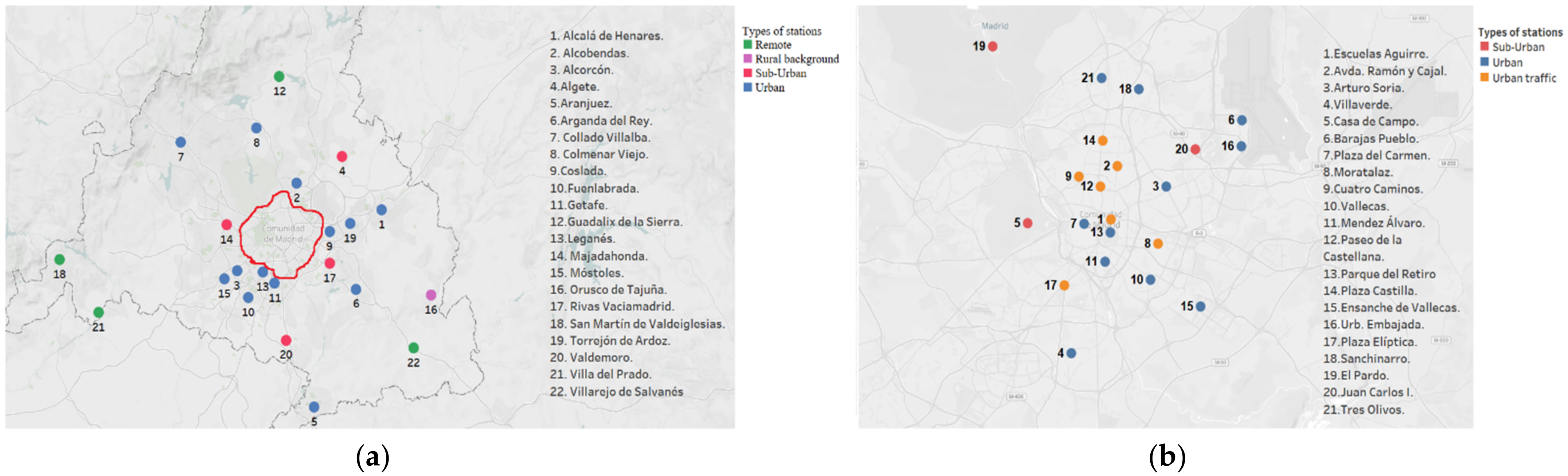
20]. To monitor and control air pollution in the city, the Madrid City Council created in 2014 the Integrated Air Quality System (IAQS). The IAQS is designed to produce a continuous flow of indicators regarding air pollution within the municipality. This information is then used for surveillance, forecasting, and information purposes. The surveillance system consists of automatic remote stations, which are spread all over the territory of the CM, as displayed in
Figure 1a,b (the latter represents an enlarged version of the area outlined by the blue line in
Figure 1a). The air quality monitoring stations are of five different kinds: urban (U), sub-urban (SU), remote (R), rural background (RB), and urban traffic (UT). Each air monitoring station is classified according to the area′s features (traffic levels, population, distance to the capital′s city center, etc.), and under no circumstances are biases among data collected at different stations according to this classification.
In this paper, we relied on air quality data collected at 43 stations of the CM, 22 of which corresponded to the network operating under the regional authority control, and the remaining 21 were monitored by the municipal air quality network of Madrid city. The data were issued, respectively, by the Atmospheric Quality Area-air Network of the autonomous region and the Atmospheric Protection Service of the Madrid Council. The time span of the sample was from 1 January 2018 to 20 June 2020, i.e., there were t = 902 observations for each air station pollutant analyzed.
Ozone was measured with ultraviolet absorption at 253.7 nm, nitrogen oxides by means of the chemiluminescence analyzer, and PM2.5 (in µg/m3) and PM10 (in µg/m3) via beta absorption technique. Chemiluminescence measurement method was applied on NO (µg/m3) and NO2 (µg/m3) pollutants, while non-dispersive infrared spectrometry was used to measure CO (µg/m3). The measurement and the processing of data were identical across stations. The daily average concentrations for CO, NO, NO2, PM10, PM2.5, and O3 were calculated throughout the 2018–2020 period using the hourly concentration of the different air pollutants.
In addition, meteorological data were downloaded from the Open Data platform of the Spanish Meteorological Agency (AEMET) via its Application Programming Interface (API). In order to associate meteorological stations with air quality monitoring stations, the closest one (using great circle distance) was chosen to obtain the meteorological variables of interest at the 41 localities where air quality monitoring stations were located: temperature (°C, minimum, mean, maximum), precipitation (mm), wind speed (kph), and Saharan dust episodes. Dust episodes were recorded at the regional level by the Ministry for Ecological Transition of Spain (MITECO) and are publicly available [
21].
2.2. Econometric Aproach
We modeled concentration of pollutant
k at station
s as a function of explanatory variables.
where
is the average daily level of pollutant
k at stations on day
t,
LDt is a binary variable that takes value 1 if the lockdown was in place, zero otherwise,
X is a full vector of control variables, and
is an error term. Parameter
βsk (marginal impact) captures the effect of
LD on pollutant
k in station s and therefore was the object of detailed analysis. The intercept and the effect of the remaining explanatory variables were captured by
and
, respectively.
We took logarithms of pollution levels because their distribution was highly right-skewed. That is, there were few days where the pollutant levels were considerably higher than the rest of the days, as we show in
Section 3.3. A second reason is that, by taking logs, all the estimated effects could be interpreted in percentage terms. A separate equation was estimated for the various pollutants considered in the paper (CO, NO, NO
2, PM
10, PM
2.5, and O
3).
Weather patterns (temperature, precipitation, wind speed) can considerably affect ground level pollutant concentrations and thereby compromise the observable effects of the LD [
2,
9,
22]. Therefore, meteorological factors were taken into account in the regression model. Specifically, vector
X included: daily maximum temperature (in °C), daily minimum temperature (in °C), daily average wind speed (in kph), and daily rainfall (in mm).
As with many other regions of the world, Spain can be affected by Saharan dust intrusion episodes, which can influence pollution levels. To capture this potential effect, X also included a dummy variable that took value 1 in the case of a Saharan dust episode. Vector X also included a binary variable to account for weekend days (Saturdays or Sundays), as economic activity and mobility were less intense during these days.
Finally, to control for the impact of Madrid Central, the low emission zone based on traffic restrictions at the very center of Madrid, an additional variable was introduced in vector X. This variable took value 1 after the creation of Madrid′s LEZ (24 November 2018) and zero otherwise. Although Madrid Central remained operational during the LD period, we set this variable to zero once the LD was decreed. This choice was intended to avoid capturing redundant characteristics, as confinement measures prevented, on their own, nearly all vehicle traffic in the Spanish capital’s city center. Moreover, municipal authorities decided not to sanction the entry into Madrid′s LEZ during the LD period in order to facilitate the mobility of workers within the area.
Finally, Equation (1) was fit to the data through ordinary least squares (OLS), a procedure that factored out, from the LD effect (, the effects of the remaining variables included in X. In other words, the LD effect reported in the paper was ceteris paribus, i.e., holding all those other factors constant.
2.3. Cluster Analysis
To obtain a typology of stations according to the initial levels of pollution and their evolution during LD, a cluster analysis was carried out. We used, as clustering variables, the average levels of pollutants in the period March–June of the years 2018 and 2019 and the percentage of variation in the LD period with respect to those average levels. The pollutants considered were NO, NO2, and O3, which were those recorded by the highest number of stations as possible. Consequently, the number of grouping variables considered was eight: average daily levels during the months of March to June of the years 2018 and 2019 of the pollutants aforementioned, relative change (in percentage) in the average daily levels of those pollutants, and comparing the average daily levels during the period of LD with the average levels during the months of March to June of the years 2018 and 2019.
The final clustering was obtained via k-means algorithm. A hierarchical cluster was made in the first place, and the optimal number of clusters was four.
2.4. Pollution Maps
Considering the average daily level of pollution before and during the COVID-19 containment period for each pollutant, the construction of pollution maps allowed us to carry out an exploratory analysis on the behavior of each of the pollutants within the CM.
Given a set of air quality stations, the pollution maps show the mean levels of NO, NO2, and O3 pollutants prior to the LD period (average daily levels in the period from 1 January 2018 to 13 March 2020) and the mean daily level during the LD period over the whole territory of Madrid region.
As the real values were limited to the stations (less than 40 points), in order to get the pollution maps, the average levels of each pollutant were estimated for the grid.
For each point in the grid, the level of each pollutant was estimated as a geographical weighted average of the pollution of all AIQ. The weights were calculated using a gaussian kernel, with adaptative bandwidth related to the distance of each grid point to the nearest monitoring station with real data [
23]. This way, the pollution level of each point depended more intensely on the closest stations and less on the farthest ones. In the case of the more isolated stations, the effect of decaying weights according to distance was less intense. A set of mathematical elements were defined.
I: Set of points in a grid of 200 × 200 points. i ∈ I.
K1: Set of pollutants upon which pollution maps are built; NO, NO2 and O3. k ∈ K1
Jk: Set of air monitoring stations that measure pollution levels of pollutant k. j ∈ Jk.
dij: Geographical distance between point i and j station.
hi: Geographical distance to the nearest monitoring station from the grid point i to j. Mathematically, it is defined as: Min{ dij }; k ∈ K, i ∈ I, j ∈ Jk.
wij: Weight associated with the distance between grid point i and air quality station j. It was calculated as: exp{−(dij/hi)2}; k ∈ K1, i ∈ I, j ∈ Jk.
w*ij: Relative weight associated with the distance between grid point i and air quality station j. It was calculated as: w*ij = w*ij/∑ wij; k ∈ K1, i ∈ I, j ∈ Jk.
Ŝik: Estimated average pollution level measured in µg/m3 of pollutant j in point k of the grid.
Analytically, for each pollutant
k, the estimated pollutant level for point
i was computed as a weighted average of the pollutant levels of the
Jk monitoring stations which had data for pollutant
k (Equation (2)).
The initial data processing was performed using the software MATLAB-R2020, while the pollution maps and clusters were developed using the R statistical package tidy, verse, and ggplot2 [
24]. The regression estimates and marginal effects were obtained using the map system and analysis tools provided by the Tableau V2020.3.1 information system/software.
2.5. Lockdown Period Determination
The CM was the area where the first COVID outbreak was detected on 6 March. By 9 March, the cases almost tripled in just 24 h, and the Madrid regional government decided to close educational institutions and delayed scheduled medical operations to stop the virus from spreading.
Faced with a growing number of deaths and the unwillingness by many citizens to follow social distancing measures, the Spanish government announced a nationwide lockdown on 13 March through the “state of alarm” [
25]. It was deemed as the strictest quarantine regime in Europe [
26]. The main objective of such drastic measures was flattening the infection curve and decreasing the disease′s reproduction number in highly populated areas [
27]. On 31 March, a further strengthening of the LD was enacted, banning all non-essential activities.
The strengthened lockdown was abandoned on 13 April, and confinement started to be relaxed between 26 April and 4 May when children and adults were allowed to perform leisure activities outdoors, and a four-stage de-escalation plan was proposed to progressively lift lockdown restrictions according to each region′s epidemiological situation. The “state of the alarm” was extended by the Spanish Congress until 21 June, when all citizens were allowed to move freely between the country′s regions, and each region took leads from the central government to decide which restrictions should remain locally.
3. Results
3.1. Meteorological Analysis
Relevant meteorological differences were evidenced in 2018, 2019, and 2020 when comparing the period between 14 March and 20 June relative to each year. According to AEMET, the average daily temperatures were approximately 3 °C lower in the north of the CM in comparison with Madrid capital and the southern regions. In year 2018, there were 31 days with daily temperatures below 10 °C in the north of the CM, while in 2019, there were 26, and in 2020, only 19 days. As for Madrid city center, year 2018 registered 21 days with average temperatures below 10 °C, while in 2019 and 2020, only 8 and 9 days were recorded, respectively. As for precipitations, year 2019 was drier in the capital′s city center than 2018 and 2020 (relative to the period between 14 March and 20 June), both in terms of total precipitation (86.9 mm in 2019, whereas in 2018 and 2020, there were 219.8 and 227.3 mm, respectively) and rainy days (in 2018, there were 29 days with daily precipitations exceeding 2 mm, 10 days in 2019, and 24 days in 2020). In northern regions, rains were heavier in 2018 and 2019, as during our study period, they recorded total precipitations of 270.6 and 100.3 mm, respectively. Nonetheless, through the 2020 “state of the alarm”, Madrid city center registered higher total precipitations (227.3 mm) than northern areas of the CM (223.2 mm). Rainy days were less frequent in northern regions in 2018 and 2020 (28 and 22 days with daily precipitations over 2 mm during the same period, respectively) than in the city center, while 2019 was characterized by a higher number of rainy days in the north (13 days).
When wind was considered, there were no huge differences, although, during the 2020 LD period, its average daily speed was slightly lower (2.79 kph) when compared to the previous two years (3 kph in 2018 and 3.25 kph in 2019).
These changes in daily mean precipitation levels in various areas of the CM during the past three years require controlling meteorological variables to properly analyze the LD measures′ impact on pollution levels [
28].
3.2. Spatial Analysis of Pollution Data
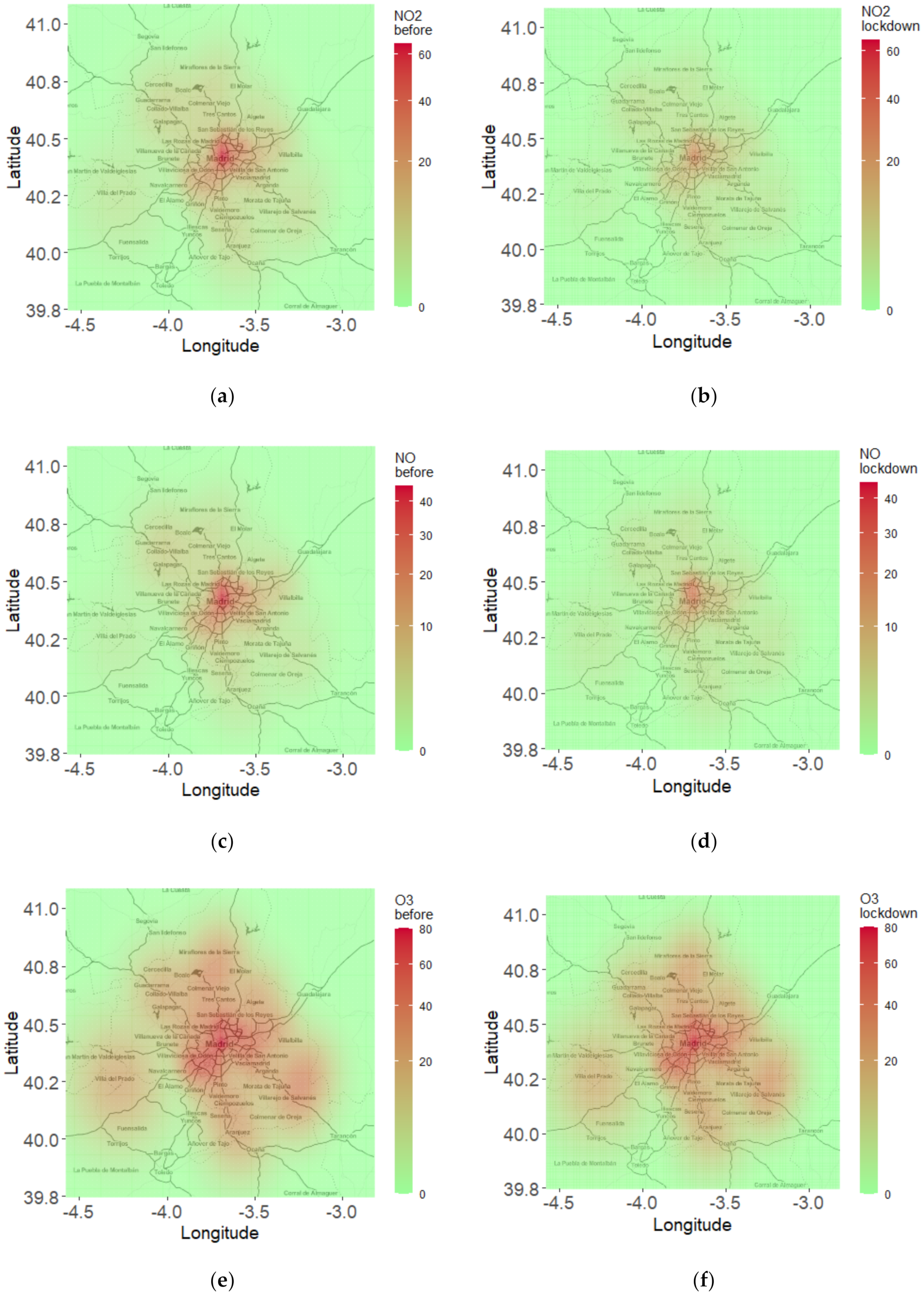
Equation (2) allowed us to represent pollution maps that outlined daily mean concentrations of NO and NO
2 pollutants. These showed a decline in pollution levels during the LD when compared to the same period in pre-COVID years (see
Figure 2a–d). These reductions were more pronounced in the central area of the CM. However, average daily concentrations of O
3 registered increased during the LD period, principally in central and southern regions of the CM (see
Figure 2e,f).
3.3. Time Trends in Pollution Levels
Figure 3 shows the evolution of NO
2 concentration in two selected stations over the sample period. The left chart corresponds to a site that is in the very center of Madrid (Plaza del Carmen), while the right chart corresponds to a distant, rural station (Villa del Prado). The creation of the LEZ in downtown Madrid and the onset of the LD period are identified by vertical lines.
The data from the urban station showed a slight decrease in NO2 concentration following the creation of the LEZ. As expected, the evolution of NO2 levels in the rural site appeared to be quite unrelated to the LEZ in Madrid center. A similar pattern was found when other urban and rural sites were considered and when we switched to other pollution particles, namely NO, NO2, PM10, and PM2.5. We interpreted these data as preliminary evidence that the LD possibly resulted in significant and asymmetric effects upon air pollutants. Still, weather conditions also play their role, and one needs to take them into account when isolating the true LD effect. In the next subsection, we turn to the full econometric setting, which allowed us to control for a variety of factors.
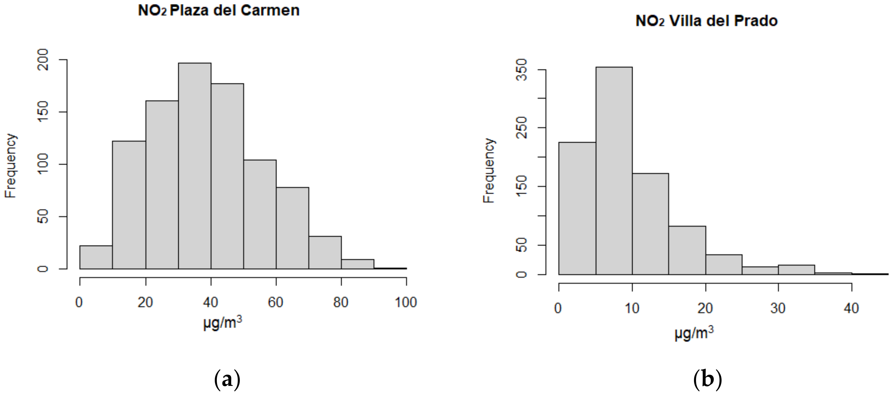
In the regression stage of the paper, the daily average of each pollutant was log transformed because their distribution was highly right-skewed. This can be seen in
Figure 4, which shows the histogram of daily levels of NO
2 at the two selected monitoring stations.
In this section, we characterize the relation between pollution levels and the explanatory variables of the model. In
Table 1, we report the results. To highlight general patterns, the estimates were averaged across stations. Since some stations do not monitor specific particles, the subsamples differed across columns. The R-squared coefficients shown in the bottom part of the table indicated that the set of explanatory variables used in the paper could account for a sizable share of the daily variation in pollution levels observed in the data. This share ranged from 37.0% (PM
2.5) up to 63.6% (NO
2).
The effect of the LD was highest on two pollutants, NO and NO2, with average reductions of 82% relative to the pre-LD period (1 January 2018–13 March 2020). Below the coefficients, we report the share of monitoring stations where the estimated parameter was found to be negative and significant at the 1% level. This condition applied to all but one station in the case of NO. Decreases in NO and NO2 were triggered by drastic reductions in social mobility during the reference period, characterized by a nearly inexistent use of means of transport (air and terrestrial).
The LD also had a significant impact on PM
10 and PM
2.5 concentrations, with average decreases of 23.4% and 18.9%, respectively. These effects were statistically significant at more than 80% of the stations. The concentration of CO was also negatively associated with the LD, although the average effect was relatively small (−3.5%). While
Table 1 is intended to capture average effects, it is also suggestive of substantial heterogeneity across stations. The LD effect on CO was negative and significant at 73% of the sample stations but positive and significant at the remaining stations. In the next section, we present a local level analysis to discuss the extent of heterogeneity with more detail. Finally, we detected an upsurge of ozone levels following the LD. The effect, 20.4% on average, was statistically significant on 73% of the sites. The increase in tropospheric O
3 pollution was due to this pollutant′s complex formation process, which was inversely influenced by changes in NO and NO
2 levels.
As for the remaining variables of the model, the daily maximum temperature was associated with higher pollution levels. This effect tended to be significant on most sites and was relatively larger when it came to tropospheric O3. Specifically, a 1 degree increase in the daily maximum temperature was associated, ceteris paribus, with a 3.2% increase in O3 concentration. This effect ranged from 0.9% (PM2.5) to 2.7% (PM10) when we inspected the remaining pollutants and turned to practically zero in the CO equation. In this case, the estimated coefficient was non-significant in most (73%) cases. These effects were practically reversed when we switched to daily minimum temperatures. Lower minimum temperatures may lead to pollution peaks, especially in winter, as they are correlated with temperature inversions during the night and with shallow depths of mixing layer during the day, also leading to very weak winds near the surface and high levels of air pollution in cities.
Wind speed was associated with significant improvements in air quality. A 1 km/h increase in wind speed induced a decrease in pollution levels that ranged from 23.1% (NO) to 2.1% (CO), the effect being negative and significant at most stations. The exception to the overall pattern was, again, O
3. In this case, air recirculation was associated with a higher concentration, a pattern that could be observed at all surveyed stations. This result matched a priori expectations, as wind transferred O
3 from those areas where it was produced (regions surrounded by heavy economic activities and intense traffic) to areas far away from metropolitan areas (rural areas), many times covering great distances [
29]. In Madrid, the highest O
3 levels were historically observed in rural areas, as the conjunction of wind and the city′s orographic features led to the displacement of this particle from urban zones (where it was generated) to areas located more than 20 km away from the city [
30].
The quantum of rain tended to be negatively associated with NO, PM2.5, and PM10, the effect being significant in at least 50% of the stations. Rain was also negatively related to CO levels, although this effect was significant in only 27% of the areas and was mildly positively related to O3 levels. Reversely, Saharan dust episodes exerted a negative effect upon air quality. The coefficient of this variable was statistically significant at most stations and ranged from 52.2% (PM10) to 2.6% (NO).
As expected, the creation of Madrid′s LEZ translated into lower average pollution levels. However, the effects were heterogeneous across pollutants and geographical areas. NO, NO
2, and O
3 concentration decreased by an average between 6.3% and 8.5%. Still, only at between 36% and 52% of the sample stations was this effect found to be significant. Moreover, Madrid′s LEZ was associated with slightly higher, not lower, average concentrations of CO, PM
2.5, and PM
10 particles. Although this effect was significant at less than one third of the monitoring stations, the positive relationship might seem surprising. However, it should not be so if we consider that CO, PM
2.5, and PM
10 are three compounds that come from different chemicals generated from direct sources (construction sites, un-paved roads, fields, smokestacks, fires, or waste incineration) but also from complex reactions of chemicals such as sulfur dioxide and nitrogen oxides in the case of PM
2.5 and PM
10 [
31,
32]. As becomes apparent in the next subsection, Madrid′s LEZ reduced pollution levels very significantly in the city center but resulted in sensitive increases in pollution in adjacent areas.
Finally, pollution decreased substantially during weekends due to lower vehicle use on Saturdays and Sundays relative to ordinary weekdays. The effect was particularly evident in the case of NO (−44.2%) and very moderate when accounting for CO and PM2.5 concentrations. On the flip side, due to the reduction in NO and NO2, tropospheric O3 levels increased by an average of 12.4% during weekends.
3.4. Local Analysis
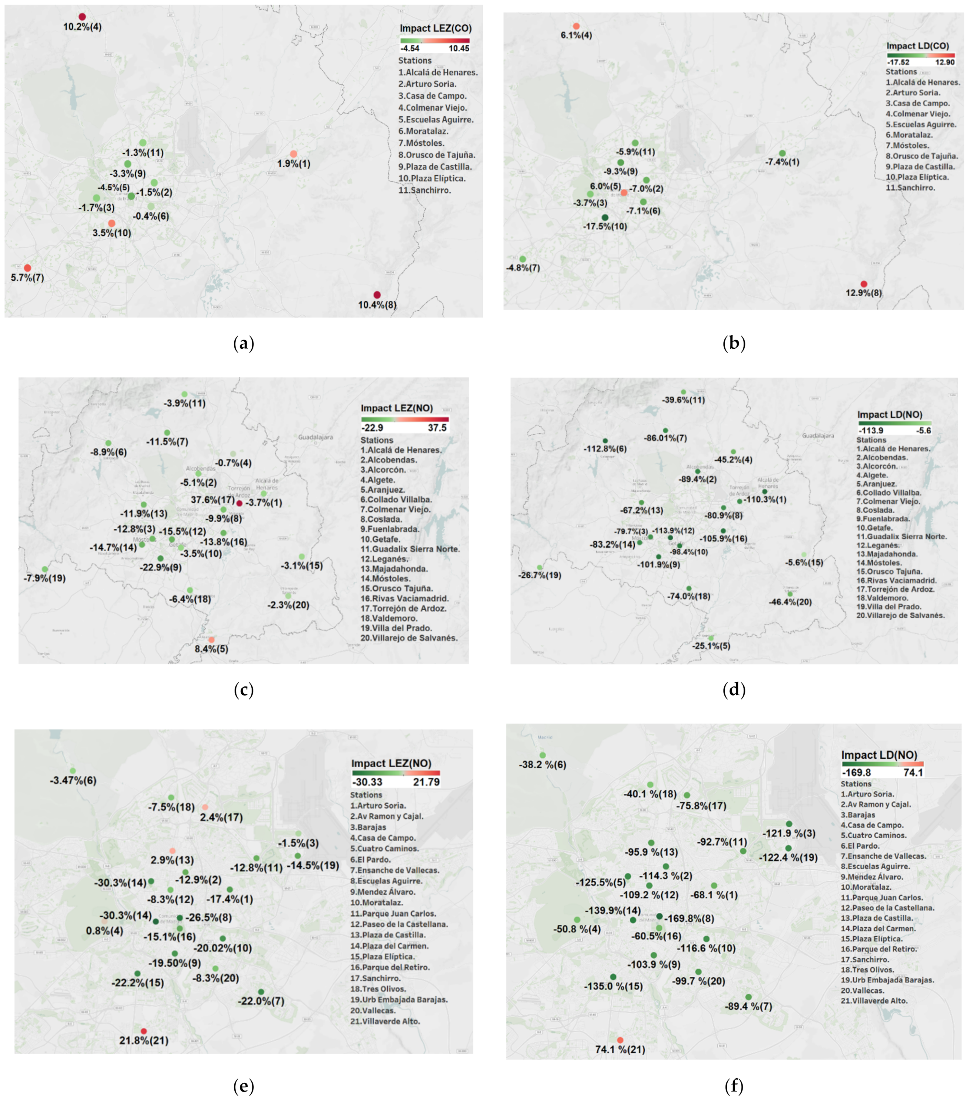
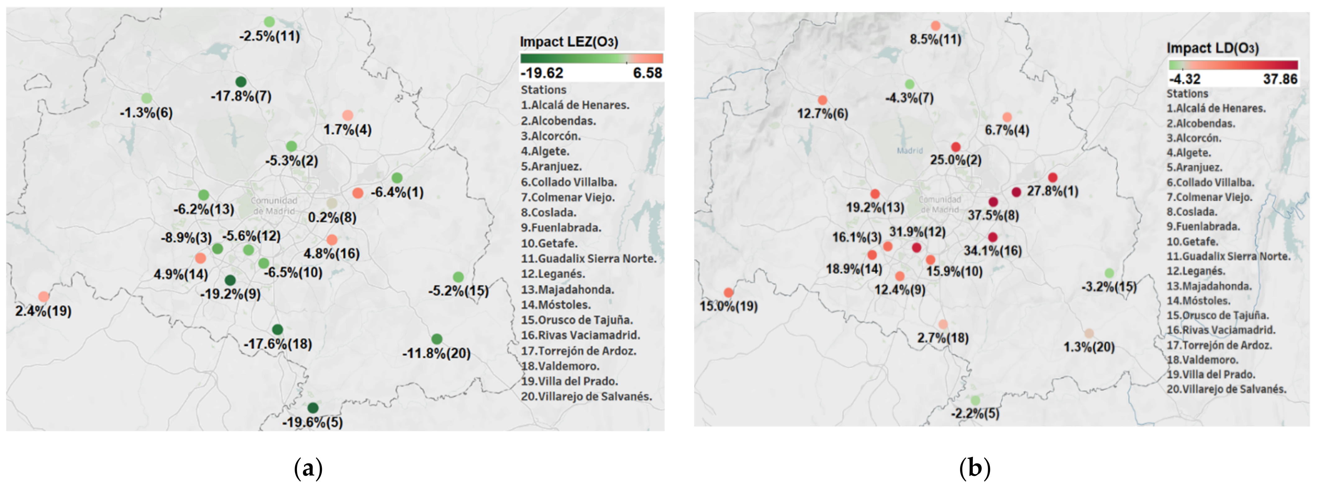
In this section, we present a local level analysis to examine to what extent the relation between pollution levels and the key variables of the model differed across sites. To provide a geographical perspective, we report the information on the maps depicted in
Figure 5 and
Figure 6. The left-hand side contains the estimates of the LEZ effect by monitoring station, while the right-hand side captures the LD effect. Dark green is used for large negative effects, while dark red denotes large positive effects.
By taking the LEZ variable as a reference against which LD effect was compared, we could contextualize the pollution-reducing scope of current traffic restrictions in Madrid. Panel (a) of
Figure 5 shows that the creation of Madrid′s LEZ resulted in very modest decreases of CO concentration within the city of Madrid and nearby areas. On two relatively distant sites (Colmenar Viejo and Orusco de Tajuña), the effect turned out to be positive and above 10%. These effects (and other unexpected effects contained in
Figure 5 and
Figure 6) were probably due to the reconfiguration of traffic patterns and human activity following the LEZ and the LD. We must recall that only 11 out of the 43 stations used in this study measured carbon monoxide levels. Using the same map, Panel (b) focuses on the LD effect upon CO. This ranged from −17.5% to −3.7% and turned to positive in three cases. The most remarkable reduction corresponded to Plaza Elíptica, a very central site characterized by heavy traffic, while changes were barely noticeable in peripheral areas. This was probably due to the intensive use during the LD period of household appliances such as stoves, heaters, and domestic biomass boilers.
The remaining panels offer a similar comparison between the LEZ and the LD effect. In these cases, we made use of the larger set of available stations and provide two maps, one for sites located outside the city of Madrid, at one for stations located within the metropolitan area. Thus, for instance, Panel (g) of
Figure 5 shows that the creation of Madrid′s LEZ resulted in large decreases of NO
2 concentration in nearby surrounding areas of Madrid. Such decreases ranged from −20.2% to −0.2%, and turned positive in only three cases. Therefore, the NO
2-reducing scope of Madrid′s LEZ was remarkable, taking into account that it comprised a small area of the city center (4.7 km
2) and that some of the stations included in the map were more than 25 km away from Madrid. However, this was not the case when we considered other pollutants such as PM
10 and PM
2.5 (Panels (e) and (i) in
Figure 5). In these cases, the LEZ effect was very limited, if not positive, in locations nearby Madrid city.
Panel (i) of
Figure 5 reports the effect of the LEZ on NO
2 concentration within the city. As expected, these estimates were larger than in Panel g), ranging from −21.1% to −0.5%. At one station (Casa de Campo), the creation of Madrid’s LEZ resulted in higher NO
2. Panels (h) and (j) also focused on NO
2 levels but now refer to the LD effect. This ranged from −105.8% to −34.8% outside the city of Madrid and from −47.5% to −124.8% within the city. The large reduction in economic activity and vehicular traffic (passenger cars, heavy duty vehicles, and buses) in central Madrid accounted for these relatively larger effects. Although Barajas (the Airport zone) and Coslada are outside Madrid, these two sites also registered considerable declines. This was so because of the plunge in air traffic during the first settlement and a reduction in road traffic in the second one.
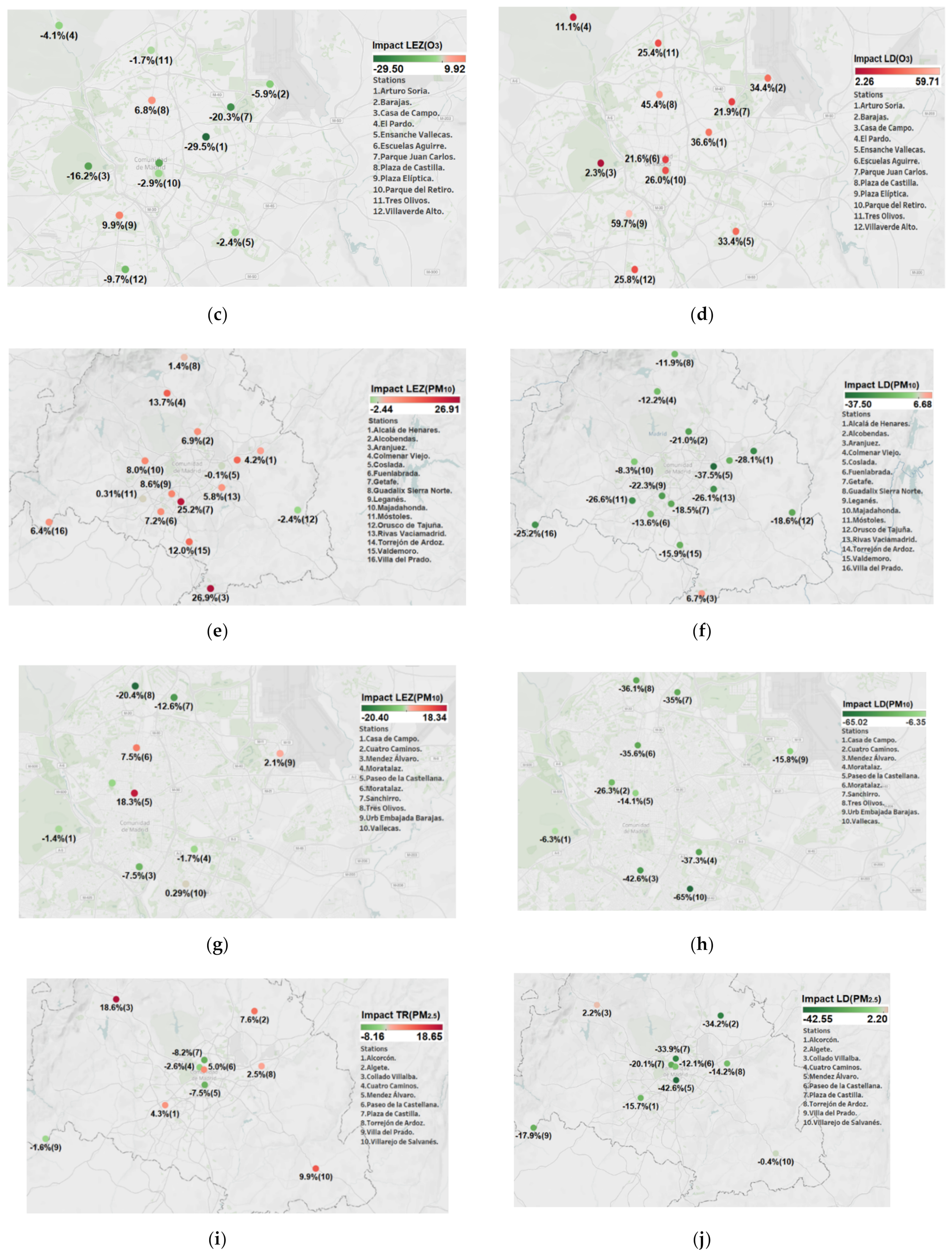
All in all, these results suggest that, first, the LD effect was, in some cases, one order of magnitude above the LEZ effect and, second, that there was substantial heterogeneity across sites. This can also be seen in
Figure 6, which focuses on O
3, PM
2.5, and PM
10. In contrast to the patterns exhibited by NO and NO
2, the largest increases in O
3 were registered within the capital and in regions traditionally affected by heavy air or road traffic, such as Barajas, Coslada, and Plaza Elíptica (Panels (b) and (d)). O
3 concentration rose only slightly in rural areas, where ozone levels were regularly high before the LD [
33].
According to the results, the behavior of CO, NO, and NO2 differed from the patterns of O3, PM10, and PM2.5 observed. The largest reductions of the first set of pollutants were found in areas characterized by intense economic activity, high social mobility, and heavy traffic. In contrast, it was mainly in rural areas where the second set of pollutants registered the most significant drops. This diverging pattern demonstrates the complexity faced by environmental policies, which typically intend to reduce the concentration of all air pollutants simultaneously.
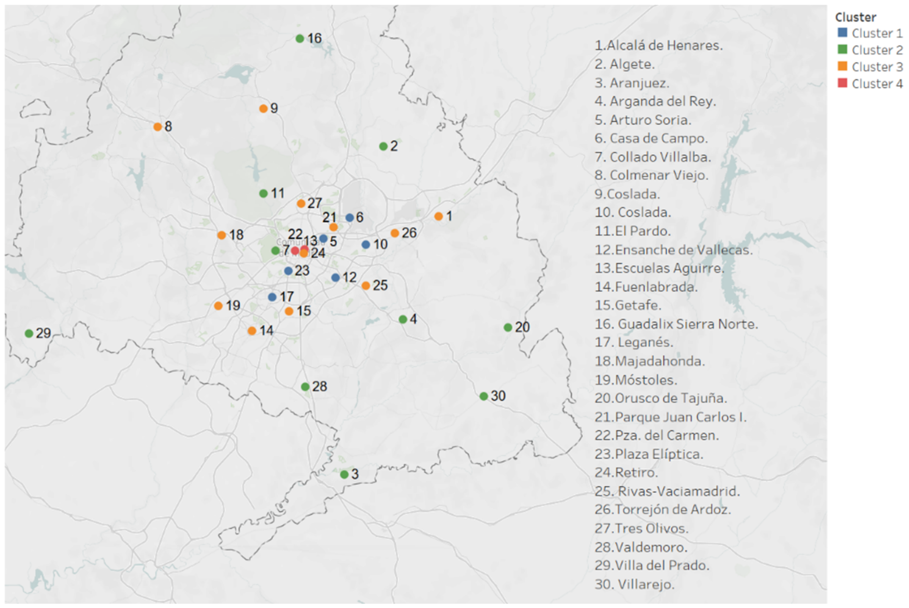
3.5. Cluster Analysis
Using clustering techniques [
34], we detected in the data four areas of pollution. Cluster 1 (blue color points on the
Figure 7) detects the area of Madrid capital characterized by reductions in NO and NO
2, whose average decreases were 21.3%, 43.6%, and a 56.9% increase in O
3 levels.
Cluster 2 (green color points on the
Figure 7) identifies basically the areas with very low emission levels due to limited traffic; among them, we included rural settlements and metropolitan areas with abundant vegetation, such as Casa de Campo and El Pardo. This means that declines in NO and NO
2 were lower and, consequently, the rise in O
3 was less pronounced than in Cluster 1 (by 13% on average).
Cluster 3 (orange color points on the
Figure 7) detects the northeast of the CM, characterized by significant percentual falls in NO and NO
2 (by 24.7% and 51%, respectively).
In Cluster 4 (red color points on the
Figure 7), two areas stand out: Escuela Aguirre and Plaza Elíptica, both with a very heavy traffic under normal circumstances, where the LD led to a plunge in NO levels by 150.8% on average.
Finally, we would like to express that, here, we characterized the changes produced in air quality during the LD. We do not pretend to attribute specifically nor quantify the effects of the LD, since other factors possibly influenced these changes, such as meteorology and regional and long transport of pollutants. An in-depth analysis is required to obtain this information accurately.
4. Discussion
This paper provides evidence that the COVID-19 induced LD resulted in significant decreases in a battery of pollutants, including NO, NO
2, PM
10, and PM
2.5. The estimates ranged from approximately −82% (NO and NO
2) to −19% (PM
2.5). Reversely, we found that the LD led to significant increases of approximately 20% in average O
3 levels. These estimates were within the range of earlier estimates reported in the literature. Thus, for instance, the previous estimates on PM
10 and PM
2.5 ranged from −50% to −5% in international studies [
4,
15] and from −28% to −8% when we considered Madrid-based data [
11,
13]. Perhaps the most remarkable difference with earlier estimates was the somewhat large effect of the LD upon NO and NO
2 found in this study of about 82%. Previous estimates ranged from −53% to −25% in international studies [
7,
15,
35] and from −56% to −30% in Spain [
12,
13,
14]. A possible explanation is that, while earlier papers were mostly based on data from March and the first fortnight of April 2020, this paper covered the entire lockdown period in Spain (March 2020–June 2020). A second difference is that the results reported here were based on econometric regression and, therefore, were controlling for potentially confounding factors. Finally, we made use of a large set of stations within the region (43), covering a 5300 km
2 surface, many of them located in Madrid city center and subject to very intense traffic and social mobility before the LD.
The reduction of pollution was more prominent in the Madrid metropolitan area than in peripheral areas, except for tropospheric ozone. This pattern was consistent with the notion that, in the metropolitan area, the disruption of economic activity induced by the LD was more intense than in other areas. Urban NO
2 is emitted by combustion processes, mostly by road traffic in urban areas, particularly by diesel engines and, to a lesser extent, gasoline vehicles, industry, power generation, and shipping [
12,
36].
Decreases in PM
10 and PM
2.5 were less pronounced than variations in NO and NO
2. This was so because particulate matter tends to persist in the air for long periods and are emitted in large quantities [
37]. Particulate matter is made up of hundreds of different chemicals that are generated from direct sources (construction sites, unpaved roads, fields, smokestacks, or fires) but also from complex reactions of chemicals such as sulfur dioxide and nitrogen oxides. While the LD had a clear impact on direct sources, its impact on indirect sources is less clear-cut [
38].
O
3 concentration increased in most settlements of the CM, except in Colmenar Viejo, Aranjuez, and Orusco Tajuña. These sites were precisely those with lowest NO and NO
2 reductions following the LD. These observations were consistent with evidence showing that decreases in NO and NO
2 levels foster O
3 formation in urban areas [
12,
30]. Moreover, decreases in NO reduce O
3 consumption (titration, NO + O
3 = NO
2 + O
2) and trigger increases in O
3 concentrations. At the same time, the usual increase of insolation and average daily temperatures from March to June led to an increase in O
3 [
31]. Such increases were exacerbated by three Saharan dust episodes in 2020 (the first from 18 March to 21 March, the second from 7 April to 9 April, and the third from 1 June to 3 June) [
12].
One of the main contributions of the paper is documenting existing differences between adjacent local areas when appraising the LD effect. The simultaneous use of ground-level data from 43 stations covering a large time span provides a clear picture of remarkable heterogeneity among sites. The effect of the LD on air quality cannot be summarized in an average sense. This also refers to Madrid′s LEZ. The results, which point to a sizable average effect ranging between −21.6% to −0.5% on NO2 at Madrid city, also suggest that the creation of Madrid′s LEZ resulted in large decreases of NO2 concentration in nearby surrounding areas of Madrid. Such decreases ranged from −20.2% to −0.2%. The NO2-reducing scope of Madrid′s LEZ was remarkable, taking into account that it comprised a small area of the city center (4.7 km2) and that some of the stations included in the map were more than 25 km away from Madrid. However, this was not the case when we considered other pollutants such as PM10 and PM2.5. This observation highlights the importance of considering a battery of pollutants when conducting this type of research.
The results were based on hourly, ground-based air quality data, while other related papers used satellite-based data [
39]. In our view, although satellites allow one to consider the spatial variability of pollutants, they have a time-limited measurement that is representative only when the satellite passes overhead and a concentration of pollutants within a vertical column, rather than those in the breathing zone [
35]. In contrast, hourly measurements fully capture temporal variability throughout the day.
5. Conclusions
The present paper examined the effect of the COVID-19 induced lockdown upon a battery of pollution particles in the Spanish community of Madrid. The average estimates ranged from approximately −82% (NO and NO2) to −3% (CO). Reversely, the COVID-19 induced lockdown raised O3 levels by an average of 20%. The data covered the period from 1 January 2018 to 20 June 2020 and, therefore, comprised the full length of the first Spanish lockdown, decreed on 13 March 2020 by the Spanish Government and lifted on June 21. This measure was deemed as the strictest quarantine regime in Europe.
One of the main contributions of the paper was to show that the lockdown effect upon pollution cannot be described as an average, for it is clearly heterogeneous across pollutants and across geographical areas. By relying on a large number (43) of monitoring stations in the region and by considering six pollutants simultaneously, the paper sheds light on the extent of heterogeneity. The reduction of pollution was more prominent in the Madrid metropolitan area than in peripheral areas, except for tropospheric ozone. This pattern, particularly evident for NO and NO2, was consistent with the notion that, in the metropolitan area, the disruption of economic activity induced by the lockdown was more intense than in other areas. Differences between urban and rural areas were smaller in the cases of PM10 and PM2.5 due to the more favorable condition or rural areas in terms of wind regimes, height, and air mass influence. Still, the results are suggestive of important differences between adjacent areas.
The results also showed that the effect of Madrid′s low emission zone (the so-called Madrid Central) upon NO2 within the city was significant, between −20% to −10%, and that surrounding areas also benefited from the initiative. However, the pollution-reducing scope of this initiative was dubious and even counterproductive in other cases, namely O3, PM10, and PM2.5 in Madrid periphery.
We can derive two policy implications from the results. Firstly, existing differences among geographical areas in the CM in terms of the evolution of air quality following the LD and the creation of Madrid′s LEZ should warn environmental policymakers that tackling the negative effects of pollution on the entire region requires a comprehensive view. There are conspicuous and heterogeneous effects that can be overlooked if the emphasis is put on the very center of Madrid. Moreover, the reduction in non-essential economic activities and mobility following the LD triggered unprecedented declines in a battery of air pollutants. However, the effects were asymmetric across pollution indicators and sites. Again, this gives further support to the notion that any successful approach to improve air quality in the region must be multidimensional.
Secondly, by comparing the LD and the LEZ effect, the paper shows that traffic restriction policies limited to the very center of Madrid can fall short when tackling pollution, especially in the cases of PM10 and PM2.5. In other words, the regional government and the City Hall should differentiate between areas characterized by permanent high concentrations of atmospheric pollutants with very harmful effects on human health (Madrid city center and its adjacent areas) and other regions where these concentrations represent a lower risk according to our cluster analysis (rural areas).
As a limitation, the paper did not control for the demographic or the orographic characteristics of the different areas. Arguably, population size, terrain contour, and wind direction are expected to play their role in determining pollutant levels. Similarly, the stance of the economic cycle may impact economic activity. During the first semester of 2020, Spain′s GDP decreased by more than 11%, where 1.5 million people lost their jobs [
40,
41]. It is likely that this unprecedented impact on household income and the labor market impacted significantly economic and pollution dynamics of the region.


 ,
, 


