Article

Ensemble Dispersion Simulation of a Point-Source Radioactive Aerosol Using Perturbed Meteorological Fields over Eastern Japan

by
Tsuyoshi Thomas Sekiyama
1,*,
Mizuo Kajino
1,2 and
Masaru Kunii
3
1
Meteorological Research Institute, Tsukuba 3050052, Japan
2
Faculty of Life and Environmental Sciences, University of Tsukuba, Tsukuba 3058572, Japan
3
Japan Meteorological Agency, Tokyo 1058431, Japan
*
Author to whom correspondence should be addressed.
Submission received: 14 April 2021 / Revised: 16 May 2021 / Accepted: 19 May 2021 / Published: 22 May 2021
(This article belongs to the Special Issue Aerosol Pollution in Asia)

Abstract

:
We conducted single-model initial-perturbed ensemble simulations to quantify uncertainty in aerosol dispersion modeling, focusing on a point-source radioactive aerosol emitted from the Fukushima Daiichi Nuclear Power Plant (FDNPP) in March 2011. The ensembles of the meteorological variables were prepared using a data assimilation system that consisted of a non-hydrostatic weather-forecast model with a 3-km horizontal resolution and a four-dimensional local ensemble transform Kalman filter (4D-LETKF) with 20 ensemble members. The emission of radioactive aerosol was not perturbed. The weather and aerosol simulations were validated with in-situ measurements at Hitachi and Tokai, respectively, approximately 100 km south of the FDNPP. The ensemble simulations provided probabilistic information and multiple case scenarios for the radioactive aerosol plumes. Some of the ensemble members successfully reproduced the arrival time and intensity of the radioactive aerosol plumes, even when the deterministic simulation failed to reproduce them. We found that a small ensemble spread of wind speed produced large uncertainties in aerosol concentrations.

1. Introduction

Ensemble simulation is a set of multiple numerical simulations that have slightly different initial conditions, boundary conditions, parameters, or models that are all geophysically plausible. Such a simulation enables the estimation of the predictability or reliability of the model simulation by providing a spread of ensemble forecasts. The simulation is most certain if the ensemble members are close to each other; otherwise, the ensemble provides a possible range of different events. Thus, probabilistic model information can be obtained from an ensemble simulation. Additionally, an ensemble simulation provides an ensemble average that is often more accurate than a deterministic single simulation because the model errors tend to be averaged out.
From a scientific viewpoint, the model predictability indicates not only the imperfection of simulation models but also the Lorenz’s deterministic chaos of Earth systems. The error growth and propagation in the model simulation depend on the chaotic advection, diffusion, precipitation, thermodynamics, and chemistry, which all should be explored in detail. From a practical perspective, probabilistic model information complements deterministic model information, especially for atmospheric forecasts. Therefore, ensemble prediction systems (EPSs) have been developed worldwide by operational weather forecast centers. These systems have adopted initial-condition ensemble simulations that are suitable for error growth evaluation.
However, it is difficult to generate the ensemble perturbations of initial conditions because randomly chosen (Monte Carlo) perturbations are likely to fade away or fail to grow through the simulations [1]. Therefore, more sophisticated perturbation methods are generally used for weather forecasts, e.g., the singular vector method or the ensemble Kalman filter method. The singular vector (SV) method was developed and implemented initially by the European Centre for Medium-range Weather Forecasting (ECMWF) [2]. This method inevitably requires the adjoint code of the forecast model. In contrast, the ensemble Kalman filter (EnKF) method, which is newer than the SV method, e.g., [3], does not require the adjoint code of the forecast model and hence has been used throughout this decade. In the EnKF method, the generation of initial perturbations is united with the data assimilation for building the initial conditions.
By contrast, atmospheric environmental EPSs have not been developed as extensively as weather EPSs, and hence the application of ensemble dispersion simulations (EDSs) has not been thoroughly explored. Most previous EDS studies were sensitivity tests validated by parameter/model ensembles, e.g., [4,5,6,7,8] that were relatively easily executable with a very small number of ensemble members, or they were Monte Carlo tests that were simply conducted with an offset modification of the initial/boundary conditions, e.g., [9,10,11,12]. Only a few EDS studies have been conducted with sophisticated initial perturbations, e.g., the ozone predictability experiments performed by Holt et al. [13] using an ensemble transform method, the CO2 source/sink inversion experiments performed by Lauvaux et al. [14] using the SV method, the schematic dispersion experiments performed by Lattner and Cervone [15] using an ensemble particle filter method, and the global aerosol dispersion experiments performed by Haszpra et al. [16] using the ECMWF global ensemble forecasts.
Here, we have investigated the model uncertainty of a regional aerosol dispersion simulation with the meteorological initial perturbation generated by the EnKF. The knowledge of the dispersion model uncertainty will provide insight regarding what model configuration is suitable for scientific and operational model usage. Unfortunately, the dispersion model uncertainty has not been well explored with ensemble simulations because (1) it is difficult to prepare meteorological perturbations with sophisticated methods like the SV and EnKF methods and (2) even if ensemble simulations are performed, it is difficult to examine the probabilistic results in detail when tracer concentration observations and emission inventories are not sufficiently available.
Therefore, we introduced two original approaches to resolve these difficulties. (1) We generated the meteorological initial ensembles ourselves using an EnKF data assimilation system with an arbitrary model resolution and domain. (2) We examined the dispersion process of the radioactive aerosol tracer (Cs-137) stemming from a point source, i.e., the Fukushima Daiichi nuclear power plant (FDNPP). Point-source pollution data are ideal for the validation of dispersion models. Especially in the case of the FDNPP accident, the emission location is exactly identified, the emission time and strength can be estimated within a reasonable range to some extent, and the aerosol tracer concentration has been accurately observed using radiation measurements. The model uncertainty will be effectively investigated with these approaches. Meanwhile, the emission term was unperturbed and thus not investigated in this study.

2. Methodology

The EnKF is an approximate treatment of the Kalman filter for application to high-dimensional systems such as the atmosphere cf. [17,18]. The Kalman filter defines an analysis as an arithmetic weighted mean of forecasts and observations, imposing a minimum variance estimation of the analysis error on the weight optimization [19]. We simultaneously obtain data assimilation products (i.e., analysis) and perturbations (i.e., ensemble members) by repeating the EnKF procedure. The analysis is the mean of the ensemble members. The perturbations generated by the EnKF are qualitatively superior to a random perturbation because they reflect the model uncertainty distribution and are flow-dependent, similar to the SV method. Furthermore, Wang et al. [20] reported that when the ensemble size is small, the EnKF method has a statistical advantage because the other methods consistently generate symmetric positive–negative paired ensemble members to keep the average value and thus cannot make statistical full use of the ensemble dimension. In contrast, the EnKF does not generate symmetric pairs but keeps the overall average. While the EnKF has several numerical implementation methods, the square root EnKF is implemented in this study. In the square root EnKF, each ensemble member retains its identity through the data assimilation cycle because its relative position in the state space among the ensemble members is invariant.
Prior to calculating the radioactive aerosol dispersion, we prepared the ensemble analysis and forecast of the meteorological variables to drive the dispersion model using an EnKF data assimilation system that was developed by Kunii [21]. This data assimilation system consists of the local ensemble transform Kalman filter (LETKF), i.e., one of the square root EnKF implementations [22], and the Japan Meteorological Agency’s non-hydrostatic regional weather forecast model (JMA-NHM) [23,24]. The LETKF method has been applied to weather forecast modeling, e.g., [21,25,26,27,28,29,30] and tracer dispersion modeling, e.g., [31,32,33,34,35,36,37,38,39,40,41].
In this study, the model domain covered eastern Japan as shown in Figure 1 and its horizontal resolution was set to 3 km, which represented a typical grid scale for the regional simulations implemented for the FDNPP accident cf. [37,39]. The model settings, such as map projection, vertical coordinate, turbulence scheme, convective scheme, and terrain features, were the same as those of the 3-km grid simulation performed by Sekiyama et al. [37,39]. The domain consists of 215 × 259 horizontal grid points in the Lambert conformal projection and 60 vertical levels including 11 levels below 1 km above ground level. The terrain features were generated from the global digital elevation data with a horizontal grid spacing of 30 arc seconds (GTOPO30) provided from the U.S. Geological Survey. The turbulence scheme was based on the improved Mellor-Yamada level 3 closure model [42,43]. A cumulus parameterization was not used in this study.
The data assimilation system was initiated at 06:00 UTC on 10 March 2011 with 20 ensemble members and a 3-h time window. The assimilation settings, such as time slots (3 h), prognostic variables (three wind components, temperature, pressure, water vapor mixing ratio, and water/ice microphysics variables), inflation scheme (adaptively multiplicative factors at each grid point), and covariance localization (1/e0.5 within 150 km in the horizontal and 0.2 natural-logarithmical p-coordinate in the vertical), were the same as those of the 3-km grid simulation performed by Sekiyama et al. [37,39]. We obtained the initial condition and the boundary conditions from the JMA operational global 15-km grid analysis.
We assimilated JMA’s operational observation dataset, which was integrated and quality-controlled for the JMA mesoscale Non-hydrostatic-model four-dimensional Variational data Assimilation system (JNoVA) [44], similarly to Kunii [21] and Sekiyama et al. [37]. Additionally, we assimilated surface wind observations acquired by the Automated Meteorological Data Acquisition System (AMeDAS) similarly to Sekiyama et al. [39]. AMeDAS is a nationwide meteorological observation network managed by JMA. The data assimilation system generated 20 ensemble members every 3 h (hereafter called ensemble analysis members) and simultaneously calculated the mean value of the ensemble members as a deterministic analysis. The forecasts were calculated by the identical JMA-NHM using these 20 ensemble members and a deterministic analysis as the initial conditions. Hereafter, these forecasts are called ensemble forecast members and a deterministic forecast, respectively.
Using the meteorological analysis or forecast outputs, Eulerian dispersion simulations were conducted with the Regional Air Quality Model version 2 (RAQM2) [45,46,47,48,49,50]. All of the radioactive Cs-137 was contained in sulfate-organics-mixed aerosol particles when it was transported in the atmosphere. The details of the modeled aerosol physics are described in work of Kajino et al. [46] and Sekiyama et al. [37,39]. Note that the RAQM2 used in this study implements simplified aerosol dynamics compared with those of Kajino et al. [46] by assuming perpetual particle size distribution similarly to Sekiyama et al. [37,39]. The combination of the JMA-NHM, the LETKF, the JNoVA+AMeDAS observations, and the RAQM2 has been successfully used for the Fukushima radioactive pollution simulation [37,39,40,41,51,52,53,54].
We used the emission scenario of the radioactive Cs-137, which was released from the FDNPP, estimated by the Japan Atomic Energy Agency (JAEA) [55,56,57]. Cs-containing sulfate-organics-mixed aerosol particles [58] were injected at every time step into a grid cell above the FDNPP. The emission scenario has been revised by JAEA several times after 2012, e.g., [59]. However, the difference between the previous ones and the revised ones is not very large in comparison with the dispersion model uncertainty (i.e., ensemble spread) of Cs-137 concentrations in this study. Since we focus on the quantification of the dispersion model uncertainty, the revision of the Cs-137 emission scenario scarcely affects the results of the uncertainty evaluation in this study.
The data assimilation cycle and the dispersion simulations were performed continuously from 11 March to 1 April 2011. The “analysis” run contained 20 ensemble simulations and one deterministic simulation. Although the analysis is only provided every 3 h, the dispersion simulations require the meteorological variables at much smaller time intervals. Therefore, the meteorological variables were generated between the 3-h analysis points by the 3-h forecast runs using the identical JMA-NHM. The variables were stored at every 10 min of simulation time and inputted into the RAQM2, and the variables were linearly interpolated during each 10-min interval. Additionally, we performed a “forecast” run for 24 h in two specific periods (15 March and 21 March, see Section 3). Each forecast was started at 21:00 local time (JST) of the previous day using the “analysis” run as the initial condition. The “forecast” run also contained 20 ensemble simulations and one deterministic simulation.

3. Results and Discussion

Here, we focused on March 15 (Period 1) and 21 (Period 2), 2011 local time to investigate the radioactive plumes that were carried landward. Nakajima et al. [60] pointed out that the plume intrusion inland occurred twice on a large scale; i.e., 15 March and 20–21 March. The comparison of the radioactive aerosol concentration was performed at the model grid corresponding to the location of Tokai, where JAEA has been operationally monitoring radionuclide concentrations and clearly detected highly radioactive plumes on both 15 and 21 March, 2011 [61]. The JAEA Tokai facilities are located approximately 100 km south of the FDNPP (Figure 1). The meteorological components were compared at the model grid corresponding to the location of Hitachi (Figure 1), where the nearest AMeDAS station (10 km north) to Tokai was located.

3.1. Period 1 (15 March 2011)

Figure 2a shows the time series of the meteorological ensemble analysis at the model surface layer (below 40 m) of the Hitachi AMeDAS station from 21:00 14 March to 21:00 15 March 2011 JST. The ensemble members are illustrated with the deterministic analysis, AMeDAS observations, and the JMA operational 5-km gridded analysis. The wind speed (u and v) ensemble had a small spread and was almost synchronized with the JMA operational analysis winds. The wind errors of the analysis members (i.e., the distance from filled circles to a bunch of black lines) were larger than the difference between the wind ensemble members (i.e., the spread width of a bunch of black lines). Figure 2b shows the forecast (initiated at 21:00 14 March 2011 JST) in which the wind ensemble had a large spread. However, the wind forecast spread was still smaller than the wind forecast error (i.e., the averaged distance from filled circles to a bunch of black lines).
The Cs-137 concentrations at the model surface layer (below 40 m) of the Tokai JAEA station are shown in Figure 3a with the JAEA observations from 21:00 14 March to 21:00 15 March 2011 JST. In contrast to the wind speed ensemble, the Cs-137 ensemble concentrations had a large spread. Some of the ensemble members successfully represented the real peak concentration but failed to represent the peak timing, appearing two hours early. The deterministic analysis underestimated the real concentration. In Figure 3b, the Cs-137 forecast members presented a larger ensemble spread for the concentration. Some of the Cs-137 forecast members presented large overestimations before and after the peak.
In this period, the radioactive aerosol plume projected from the FDNPP to the south, coastwise, and then swept across Tokai (Figure 4). The percentile distribution of the 20 ensemble members was narrow in the analysis (Figure 4a) but relatively broad in the forecast (Figure 4b), which was in agreement with the time series of the ensemble analysis/forecast concentrations at Tokai that are shown in Figure 3. The threshold (15 Bq/m3) used here was defined as the half value of the air quality standard of Japan’s radioisotope regulations. The percentile distribution of aerosol concentrations can be usefully applied to probabilistic forecasts such as the chance-of-rain forecast. The probabilistic forecasts provide multiple scenarios for environmental pollution or disasters. Generally, the accuracy of the forecast decreases with time, and consequently the percentile distribution tends to diffuse with time. Figure 4 shows that the forecast percentile distributions were very similar to the analysis percentile distributions in the short forecasts (02:00 15 March and 06:00 15 March), indicating the high accuracy of the forecast. However, the distributions were less similar in the longer forecast (10:00 15 March), in which the forecast percentile distribution was diffused.
The ensemble analysis of the surface wind speed (u and v) exhibited a relatively small spread, which was usually less than 1 m/s even though the analysis errors (i.e., analysis minus observation) were generally 1 or 2 m/s. For example, the relative standard deviation (RSD) of the ensemble analysis for the specific 4 h during Period 1 (02:00–08:00 15 March) was 5% on average (Table 1). By contrast, the ensemble of the surface Cs-137 concentration had a large spread, in which some members occasionally presented almost zero concentrations, whereas others presented very high concentrations. The RSD of the Cs-137 concentration analysis for the same time periods was 93 % on average (Table 1). This result indicates that a small ensemble spread in meteorology produces a large ensemble spread for aerosol concentration. Thus, the uncertainty on the concentration is amplified in comparison with that on the wind field.
The ensemble forecast exhibited the same behavior as the analysis. The ensemble spread was relatively small in the meteorological simulation and very large in the dispersion simulation. The forecast RSD of the wind speed for the same time periods mentioned above (02:00–08:00 15 March) was 7% on average (Table 1). In contrast, the forecast RSD of the Cs-137 concentration was 82% (Table 1). A comparison of the analysis and forecast RSDs indicates that the errors of the dispersion models are not linearly correlated with the errors of the meteorological models.

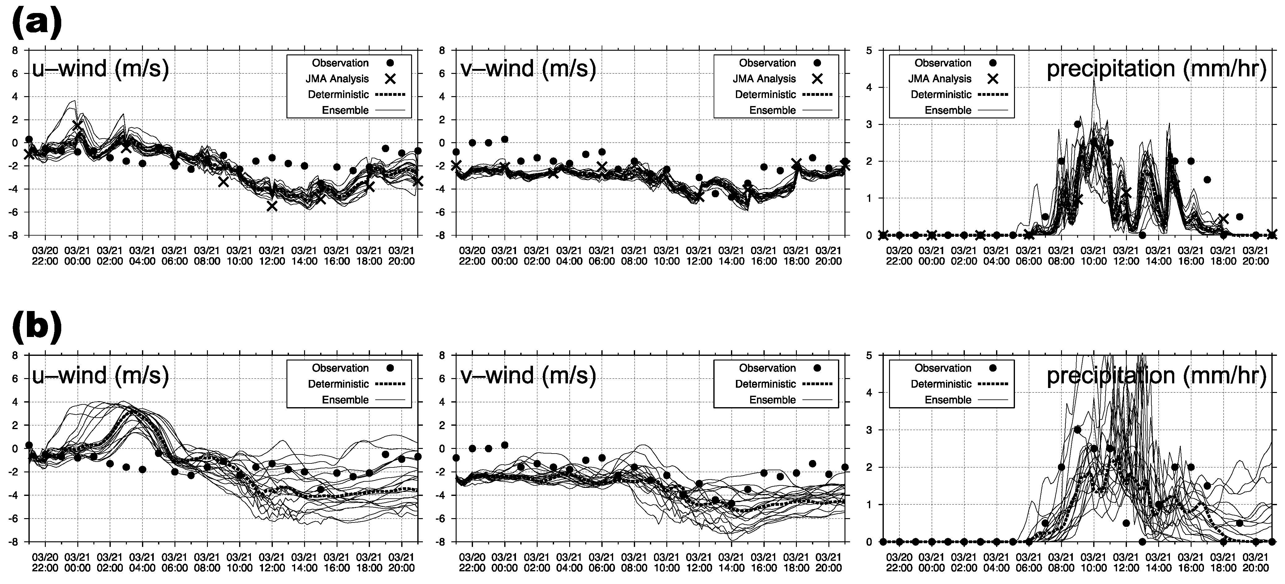
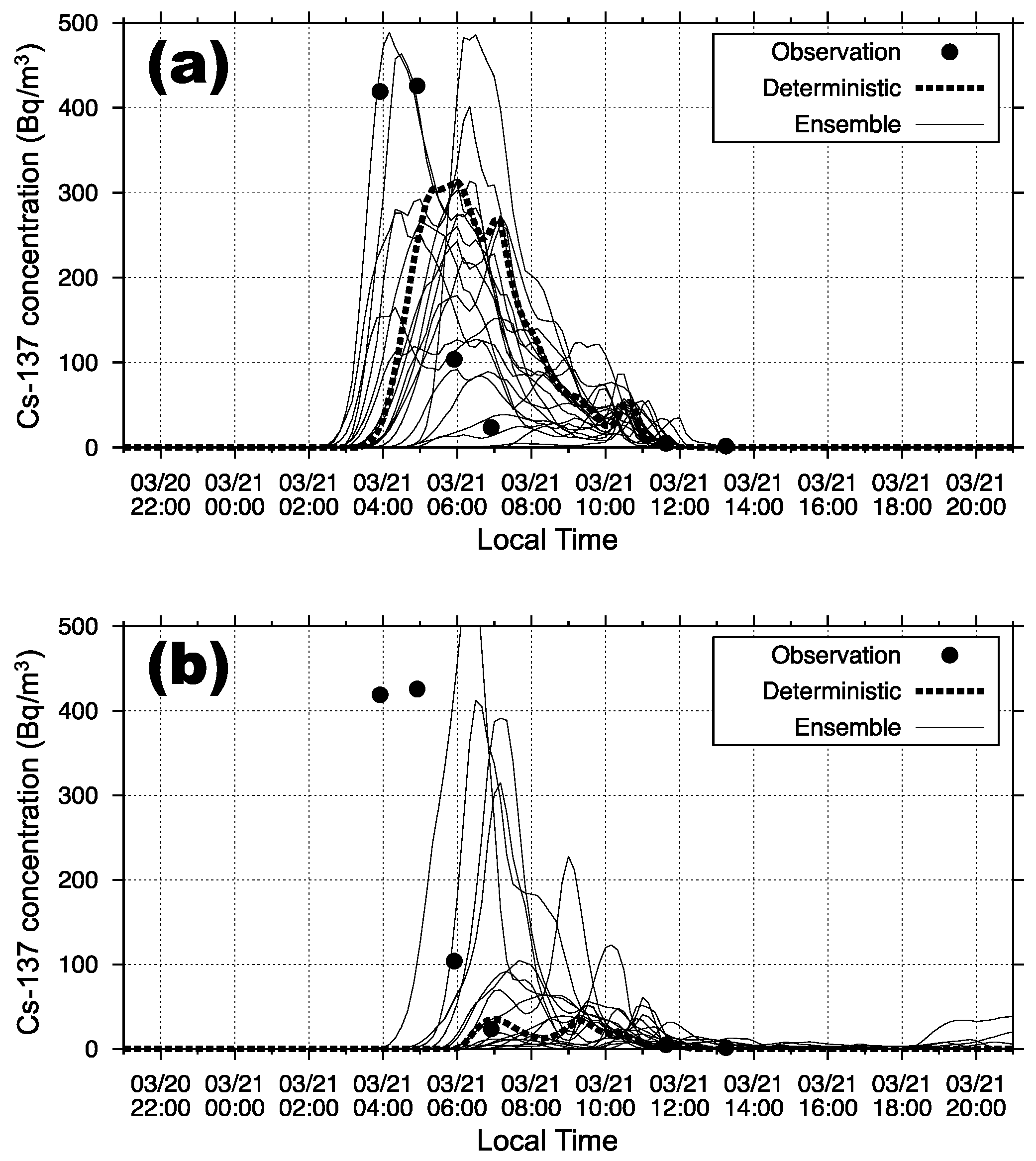
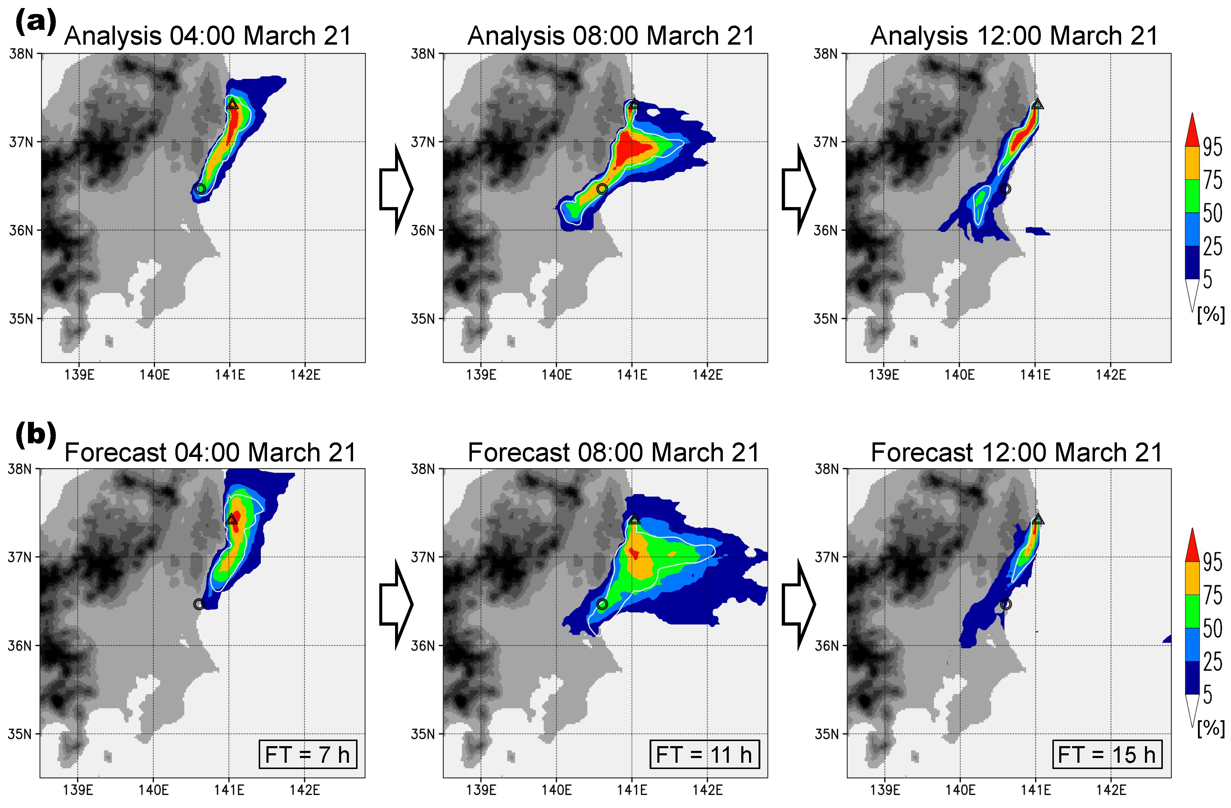
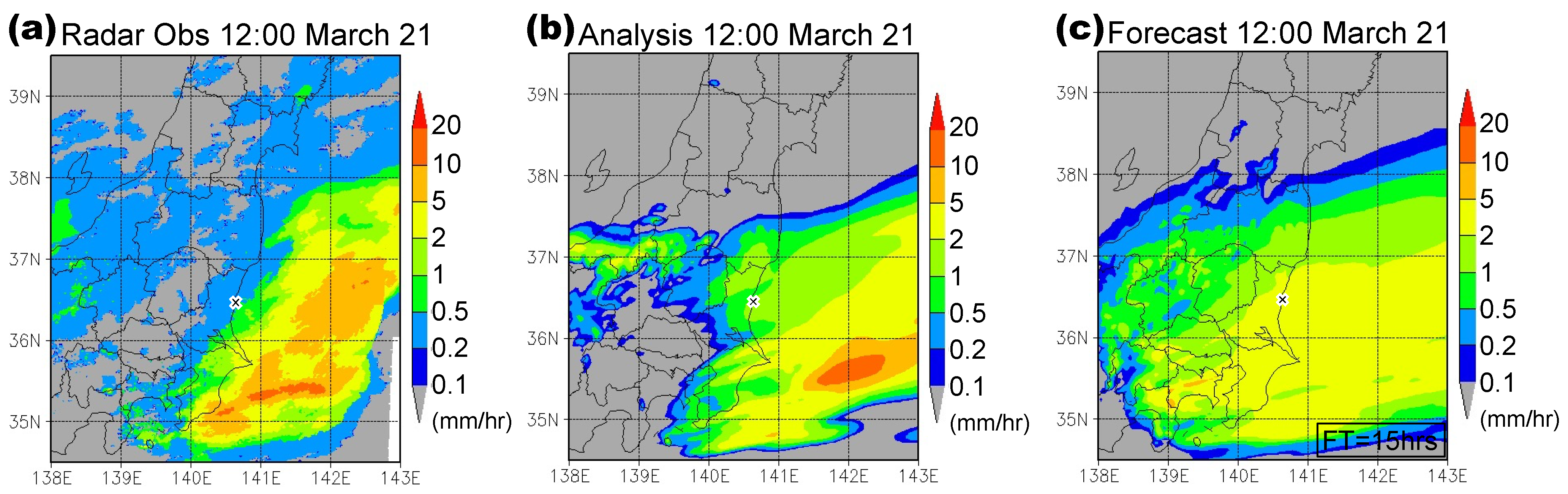
3.2. Period 2 (21 March 2011)

In comparison with Period 1, the ensemble spreads tended to be larger in Period 2. Figure 5 shows time series of the meteorological ensembles at the Hitachi AMeDAS station similar to those in Figure 2 but for the time period from 21:00 20 March to 21:00 21 March, 2011 JST. Note that it was raining or snowing on this day in a wide area of eastern Japan. As seen in Figure 5b, the ensemble forecast (initiated at 21:00 20 March 2011 JST) presented chaotic motions of the wind speed (u and v). Furthermore, the ensemble spread of the precipitation forecast was extremely large.
The time series of the Cs-137 concentrations at the Tokai JAEA station are shown in Figure 6 similar to those in Figure 3, except that they are in the time period from 21:00 20 March to 21:00 21 March 2011 JST. The ensemble spreads were very large, similar to those in Period 1. As shown in Figure 6a, the deterministic analysis failed to represent the peak timing with a two-hour delay. However, some of the ensemble analysis members successfully represented the real peak timing and concentration. In contrast to the deterministic analysis, the deterministic forecast completely failed to represent the plume arrival (Figure 6b). Many of the ensemble forecast members behaved similarly to the deterministic forecast. This failure was caused by the wet deposition (below-cloud scavenging) that occurred before the plume arrived at Tokai in the forecast simulations.
In Period 2, the RSD of the wind speed analysis for the specified 4 h (04:00–10:00 21 March) was 10% on average (Table 1). However, the RSD of the Cs-137 concentration analysis for the same time periods was 77% on average (Table 1). These scores also indicate that the uncertainty on the concentration is amplified as shown in Period 1. This finding implies that if we deterministically pursue an accurate dispersion, it is necessary to unrealistically increase the accuracy of the meteorological simulation. As expected, the percentile distributions of the Cs-137 concentration (Figure 7) tended to be broader than those in Period 1 in both the analysis and forecast before raining (approximately 08:00 JST). The percentile distributions rapidly shrank after the rain because the radioactive aerosols were deposited through precipitation. In the forecast, the precipitation area or timing was slightly shifted from the actual values, and consequently, the distribution of wet deposition was inadequately distorted.
The forecast RSD of the wind speed for the same time periods was 23% on average and that of the Cs-137 concentration was 235% (Table 1). The extremely large forecast errors of the Cs-137 concentration were caused by the forecast errors of the precipitation (not only the strength but also the timing). Specifically, the deterministic forecast almost completely failed to reproduce the Cs-137 plume arriving at Tokai (Figure 6b). In comparison with the extreme error of the Cs-137 concentration, the precipitation error was moderate as shown in the right panel of Figure 5b.
On this day, light precipitation was widespread over Japan (Figure 8a; derived from the JMA Radar/rain-gauge Analyzed Precipitation data [62]) and reasonably reproduced by the deterministic analysis (Figure 8b). The deterministic forecast (Figure 8c) produced a different distribution from the observed values (Figure 8a) and the analyzed values (Figure 8b). This difference caused the Cs-137 concentration to have a high error, indicating that the error of the dispersion models is not only amplified in comparison with the error of the wind speed but also crucially magnified by the error of the precipitation because of the high sensitivity of aerosol deposition on precipitation. However, even so, some of the ensemble members were successful in reproducing the high concentration at Tokai. This is the advantage of ensemble simulations.

4. Conclusions

We conducted ensemble simulations for the dispersion of a point-source aerosol using perturbed meteorological fields. The ensemble simulations provided probabilistic information and multiple case scenarios for the aerosol dispersion. We found that a small ensemble spread of wind speed resulted in a large uncertainty in aerosol concentrations, i.e., the uncertainty on the aerosol dispersion was amplified in comparison with that on the wind simulation. This finding implies that a high accuracy of dispersion modeling requires much higher accuracy of meteorological modeling, thus representing a limitation of deterministic dispersion simulations for analyzing/predicting the location and intensity of aerosol plumes. Therefore, the probabilistic information of ensemble simulations exhibits great potential for aerosol analysis and prediction.
The deterministic simulation did not provide the best analysis/prediction in this study. However, some of the ensemble members successfully reproduced the arrival time and intensity of the aerosol plumes. With only a deterministic simulation, it is not possible to account for another event. Regrettably, in the field of atmospheric chemistry modeling, too much emphasis has been placed on deterministic simulations uncritically. The usefulness of ensemble simulations should be recognized to a greater extent.
The errors in the aerosol simulation were not only cumulative with the errors in wind speed simulation but also crucially magnified by the errors in the precipitation simulation because of the dependence of aerosol deposition on precipitation. Although the single-model initial-perturbed ensemble simulation as used in this study is a powerful tool to explore probabilistic analysis/prediction, the limitations of the single-model simulation should also be considered because the single-model simulation implements only a single module for the precipitation.

Author Contributions

Conceptualization, T.T.S.; Methodology, T.T.S., M.K. (Mizuo Kajino), and M.K. (Masaru Kunii); Software, M.K. (Mizuo Kajino) and M.K. (Masaru Kunii); Validation, T.T.S.; Formal Analysis, T.T.S.; Investigation, T.T.S.; Data Curation, T.T.S. and M.K. (Mizuo Kajino); Writing—Original Draft Preparation, T.T.S.; Writing—Review & Editing, T.T.S.; Visualization, T.T.S.; Funding Acquisition, T.T.S. and M.K. (Mizuo Kajino). All authors have read and agreed to the published version of the manuscript.

Funding

This work was supported by the Environment Research and Technology Development Fund (1-1802) at the Environmental Restoration and Conservation Agency and by JSPS KAKENHI Grant Numbers 24340115, 17K00533, 19H01155, and 21H03593.

Institutional Review Board Statement

Not applicable.

Informed Consent Statement

Not applicable.

Data Availability Statement

We thank M. Chino of JAEA for providing Cs-137 emission inventory data from their published papers [55,56,57]. We thank JAEA for providing their Cs-137 observation data from their published technical note [61]. The JMA data are available freely at their website or can be purchased via the Japan Meteorological Business Support Center. The numerical model source codes used in this study are available under a collaborative framework between MRI and related institutes/universities. The ensemble analysis and forecast data generated in this study is available on request to the corresponding author.

Acknowledgments

We greatly acknowledge K. Saito of JMA and T. Iwasaki of Tohoku University for their help and encouragement. We deeply thank S. Koizumi for his technical support.

Conflicts of Interest

The authors declare no conflict of interest.

References

  1. Hoffman, R.N.; Kalnay, E. Lagged average forecasting, an alternative to Monte Carlo forecasting. Tellus A 1983, 35, 100–118. [Google Scholar] [CrossRef]
  2. Molteni, F.; Buizza, R.; Palmer, T.N.; Petroliagis, T. The new ECMWF ensemble prediction system: Methodology and validation. Q. J. R. Meteorol. Soc. 1996, 122, 73–119. [Google Scholar] [CrossRef]
  3. Houtekamer, P.L.; Mitchell, H.L.; Deng, X. Model Error Representation in an Operational Ensemble Kalman Filter. Mon. Weather Rev. 2009, 137, 2126–2143. [Google Scholar] [CrossRef]
  4. Galmarini, S.; Bianconi, R.; Klug, W.; Mikkelsen, T.; Addis, R.; Andronopoulos, S.; Astrup, P.; Baklanov, A.; Bartniki, J.; Bartzis, J.C.; et al. Ensemble dispersion forecasting, Part 1: Concept, Approach and indicators. Atmos. Environ. 2004, 38, 4607–4617. [Google Scholar] [CrossRef]
  5. Monache, L.D.; Deng, X.; Zhou, Y.; Stull, R. Ozone ensemble forecasts: 1. A new ensemble design. J. Geophys. Res. 2006, 111, D05307. [Google Scholar]
  6. Hegarty, J.; Draxler, R.R.; Stein, A.F.; Brioude, J.; Mountain, M.; Eluszkiewicz, J.; Nehrkorn, T.; Ngan, F.; Andrews, A. Evaluation of Lagrangian Particle Dispersion Models with Measurements from Controlled Tracer Releases. J. Appl. Meteorol. Clim. 2013, 52, 2623–2637. [Google Scholar] [CrossRef]
  7. Angevine, W.M.; Brioude, J.; McKeen, S.; Holloway, J.S. Uncertainty in Lagrangian pollutant transport simulations due to meteorological uncertainty from a mesoscale WRF ensemble. Geosci. Model Dev. 2014, 7, 2817–2829. [Google Scholar] [CrossRef] [Green Version]
  8. Draxler, R.; Arnold, D.; Chino, M.; Galmarini, S.; Hort, M.; Jones, A.; Leadbetter, S.; Malo, A.; Maurer, C.; Rolph, G.; et al. World Meteorological Organization’s model simulations of the radionuclide dispersion and deposition from the Fukushima Daiichi nuclear power plant accident. J. Environ. Radioact. 2015, 139, 172–184. [Google Scholar] [CrossRef] [PubMed]
  9. Dabberdt, W.F.; Miller, E. Uncertainty, ensembles and air quality dispersion modeling: Applications and challenges. Atmos. Environ. 2000, 34, 4667–4673. [Google Scholar] [CrossRef]
  10. Hanna, S.R.; Lu, Z.; Frey, H.C.; Wheeler, N.; Vukovich, J.; Arunachalam, S.; Femau, M.; Hansen, D.A. Uncertainties in predicted ozone concentrations due to input uncertainties for the UAM-V photochemical grid model applied to the July 1995 OTAG domain. Atmos. Environ. 2001, 35, 891–903. [Google Scholar] [CrossRef]
  11. Draxler, R.R. Evaluation of an Ensemble Dispersion Calculation. J. Appl. Meteorol. 2003, 42, 308–317. [Google Scholar] [CrossRef]
  12. Zhang, F.; Bei, N.; Nielsen-Gammon, J.W.; Li, G.; Zhang, R.; Stuart, A.; Aksoy, A. Impacts of meteorological uncertainties on ozone pollution predictability estimated through meteorological and photochemical ensemble forecasts. J. Geophys. Res. 2007, 112, D04304. [Google Scholar] [CrossRef]
  13. Holt, T.; Pullen, J.; Bishop, C.H. Urban and ocean ensembles for improved meteorological and dispersion modelling of the coastal zone. Tellus A 2009, 61, 232–249. [Google Scholar] [CrossRef]
  14. Lauvaux, T.; Pannekoucke, O.; Sarrat, C.; Chevallier, F.; Ciais, P.; Noilhan, J.; Rayner, P.J. Structure of the transport uncertainty in mesoscale inversions of CO2 sources and sinks using ensemble model simulations. Biogeosciences 2009, 6, 1089–1102. [Google Scholar] [CrossRef] [Green Version]
  15. Lattner, A.D.; Cervone, G. Ensemble modeling of transport and dispersion simulations guided by machine learning hypotheses generation. Comput. Geosci. 2012, 48, 267–279. [Google Scholar] [CrossRef]
  16. Haszpra, T.; Lagzi, I.; Tél, T. Dispersion of aerosol particles in the free atmosphere using ensemble forecasts. Nonlinear Process. Geophys. 2013, 20, 759–770. [Google Scholar] [CrossRef] [Green Version]
  17. Evensen, G. The Ensemble Kalman Filter: Theoretical formulation and practical implementation. Ocean Dyn. 2003, 53, 343–367. [Google Scholar] [CrossRef]
  18. Kalnay, E. Atmospheric Modeling, Data Assimilation and Predictability; Cambridge University Press: Cambridge, UK, 2003. [Google Scholar]
  19. Kalman, R.E. A New Approach to Linear Filtering and Prediction Problems. Trans. ASME J. Basic Eng. 1960, 82D, 35–45. [Google Scholar] [CrossRef] [Green Version]
  20. Wang, X.; Bishop, C.H.; Julier, S.J. Which Is Better, an Ensemble of Positive–Negative Pairs or a Centered Spherical Simplex Ensemble? Mon. Weather Rev. 2004, 132, 1590–1605. [Google Scholar] [CrossRef]
  21. Kunii, M. Mesoscale Data Assimilation for a Local Severe Rainfall Event with the NHM–LETKF System. Weather Forecast. 2014, 29, 1093–1105. [Google Scholar] [CrossRef]
  22. Hunt, B.R.; Kostelich, E.J.; Szunyogh, I. Efficient data assimilation for spatiotemporal chaos: A local ensemble transform Kalman filter. Phys. D 2007, 230, 112–126. [Google Scholar] [CrossRef] [Green Version]
  23. Saito, K.; Fujita, T.; Yamada, Y.; Ishida, J.; Kumagai, Y.; Aranami, K.; Ohmori, S.; Nagasawa, R.; Kumagai, S.; Muroi, C.; et al. The operational JMA nonhydrostatic mesoscale model. Mon. Weather Rev. 2006, 134, 1266–1298. [Google Scholar] [CrossRef]
  24. Saito, K.; Ishida, J.; Aranami, K.; Hara, T.; Segawa, T.; Narita, M.; Honda, Y. Nonhydrostatic atmospheric models operational development at JMA. J. Meteorol. Soc. Jpn. 2007, 85B, 271–304. [Google Scholar] [CrossRef] [Green Version]
  25. Miyoshi, T.; Aranami, K. Applying a four-dimensional local ensemble transform Kalman filter (4D-LETKF) to the JMA nonhydrostatic model (NHM). SOLA 2006, 2, 128–131. [Google Scholar] [CrossRef] [Green Version]
  26. Miyoshi, T.; Yamane, S. Local ensemble transform Kalman filtering with an AGCM at a T159/L48 resolution. Mon. Weather Rev. 2007, 135, 3841–3861. [Google Scholar] [CrossRef] [Green Version]
  27. Miyoshi, T. The Gaussian approach to adaptive covariance inflation and its implementation with the local ensemble transform Kalman filter. Mon. Weather Rev. 2011, 139, 1519–1535. [Google Scholar] [CrossRef]
  28. Miyoshi, T.; Kunii, M. The local ensemble transform Kalman filter with the Weather Research and Forecast Model: Experiments with real observations. Pure Appl. Geophys. 2012, 169, 321–333. [Google Scholar] [CrossRef]
  29. Kunii, M.; Miyoshi, T.; Kalnay, E. Estimating the impact of real observations in regional numerical weather prediction using an ensemble Kalman filter. Mon. Weather Rev. 2012, 140, 1975–1987. [Google Scholar] [CrossRef]
  30. Kunii, M.; Miyoshi, T. Including uncertainties of sea surface temperature in an ensemble Kalman filter: A case study of Typhoon Sinlaku (2008). Weather Forecast. 2012, 27, 1586–1597. [Google Scholar] [CrossRef]
  31. Miyazaki, K.; Eskes, H.J.; Sudo, K.; Takigawa, M.; van Weele, M.; Boersma, K.F. Simultaneous assimilation of satellite NO2, O3, CO, and HNO3 data for the analysis of tropospheric chemical composition and emissions. Atmos. Chem. Phys. 2012, 12, 9545–9579. [Google Scholar] [CrossRef] [Green Version]
  32. Nakamura, T.; Akiyoshi, H.; Deushi, M.; Miyazaki, K.; Kobayashi, C.; Shibata, K.; Iwasaki, T. A multimodel comparison of stratospheric ozone data assimilation based on an ensemble Kalman filter approach. J. Geophys. Res. Atmos. 2013, 118, 3848–3868. [Google Scholar] [CrossRef]
  33. Yumimoto, K.; Murakami, H.; Tanaka, T.Y.; Sekiyama, T.T.; Ogi, A.; Maki, T. Forecasting of Asian Dust Storm during 10-13 May in 2011 with an Ensemble-based Data Assimilation System. Particuology 2016, 28, 121–130. [Google Scholar] [CrossRef]
  34. Sekiyama, T.T.; Tanaka, T.Y.; Shimizu, A.; Miyoshi, T. Data assimilation of CALIPSO aerosol observations. Atmos. Chem. Phys. 2010, 10, 39–49. [Google Scholar] [CrossRef] [Green Version]
  35. Sekiyama, T.T.; Deushi, M.; Miyoshi, T. Operation-oriented ensemble data assimilation of total column ozone. SOLA 2011, 7, 41–44. [Google Scholar] [CrossRef] [Green Version]
  36. Sekiyama, T.T.; Tanaka, T.Y.; Maki, T.; Mikami, M. The effects of snow cover and soil moisture on Asian dust: II. Emission estimation by lidar data assimilation. SOLA 2011, 7A, 40–43. [Google Scholar] [CrossRef] [Green Version]
  37. Sekiyama, T.T.; Kunii, M.; Kajino, M.; Shimbori, T. Horizontal Resolution Dependence of Atmospheric Simulations of the Fukushima Nuclear Accident Using 15-km, 3-km, and 500-m Grid Models. J. Meteorol. Soc. Jpn 2015, 93, 45–60. [Google Scholar] [CrossRef] [Green Version]
  38. Sekiyama, T.T.; Yumimoto, K.; Tanaka, T.Y.; Nagao, T.; Kikuchi, M.; Murakami, H. Data Assimilation of Himawari-8 Aerosol Observations: Asian Dust Forecast in June 2015. SOLA 2016, 12, 86–90. [Google Scholar] [CrossRef] [Green Version]
  39. Sekiyama, T.T.; Kajino, M.; Kunii, M. The Impact of Surface Wind Data Assimilation on the Predictability of Near-Surface Plume Advection in the Case of the Fukushima Nuclear Accident. J. Meteorol. Soc. Jpn 2017, 95, 447–454. [Google Scholar] [CrossRef] [Green Version]
  40. Sekiyama, T.T.; Iwasaki, T. Mass flux analysis of 137Cs plumes emitted from the Fukushima Daiichi Nuclear Power Plant. Tellus B 2018, 70, 1–11. [Google Scholar] [CrossRef] [Green Version]
  41. Sekiyama, T.T.; Kajino, M. Reproducibility of Surface Wind and Tracer Transport Simulations over Complex Terrain Using 5-, 3-, and 1-km-Grid Models. J. Appl. Meteor. Climatol. 2020, 59, 937–952. [Google Scholar] [CrossRef] [Green Version]
  42. Nakanishi, M.; Niino, H. An improved Mellor-Yamada level 3 model with condensation physics: Its design and verification. Bound. Layer Meteorol. 2004, 112, 1–31. [Google Scholar] [CrossRef]
  43. Nakanishi, M.; Niino, H. An improved Mellor-Yamada level-3 model: Its numerical stability and application to a regional prediction of advection fog. Bound. Layer Meteorol. 2006, 119, 397–407. [Google Scholar] [CrossRef]
  44. Honda, Y.; Nishijima, M.; Koizumi, K.; Ohta, Y.; Tamiya, K.; Kawabata, T.; Tsuyuki, T. A pre-operational variational data assimilation system for a non-hydrostatic model at the Japan Meteorological Agency: Formulation and preliminary results. Q. J. R. Meteorol. Soc. 2005, 131, 3465–3475. [Google Scholar] [CrossRef]
  45. Adachi, K.; Kajino, M.; Zaizen, Y.; Igarashi, Y. Emission of spherical cesium-bearing particles from an early stage of the Fukushima nuclear accident. Sci. Rep. 2013, 3, 2554. [Google Scholar] [CrossRef] [Green Version]
  46. Kajino, M.; Inomata, Y.; Sato, K.; Ueda, H.; Han, Z.; An, J.; Katata, G.; Deushi, M.; Maki, T.; Oshima, N.; et al. Development of the RAQM2 aerosol chemical transport model and predictions of the Northeast Asian aerosol mass, size, chemistry, and mixing type. Atmos. Chem. Phys. 2012, 12, 11833–11856. [Google Scholar] [CrossRef] [Green Version]
  47. Kajino, M.; Sekiyama, T.T.; Mathieu, A.; Irène, K.; Périllat, R.; Quélo, D.; Quérel, A.; Saunier, O.; Adachi, K.; Girard, S.; et al. Lessons learned from atmospheric modeling studies after the Fukushima nuclear accident: Ensemble simulations, data assimilation, elemental process modeling, and inverse modeling. Geochem. J. 2018, 52, 85–101. [Google Scholar] [CrossRef] [Green Version]
  48. Kajino, M.; Deushi, M.; Sekiyama, T.T.; Oshima, N.; Yumimoto, K.; Tanaka, T.; Ching, J.; Hashimoto, A.; Yamamoto, Y.; Ikegami, M.; et al. NHM-Chem, the Japan Meteorological Agency’s Regional Meteorology-Chemistry Model: Model Evaluations toward the Consistent Predictions of the Chemical, Physical, and Optical Properties of Aerosols. J. Meteorolo. Soc. Jpn 2019, 97, 337–374. [Google Scholar] [CrossRef] [Green Version]
  49. Kajino, M.; Sekiyama, T.T.; Igarashi, Y.; Katata, G.; Sawada, M.; Adachi, K.; Zaizen, Y.; Tsuruta, H.; Nakajima, T. Deposition and dispersion of radio-cesium released due to the Fukushima nuclear accident: Sensitivity to meteorological models and physical modules. J. Geophys. Res. 2019, 124, 1823–1845. [Google Scholar] [CrossRef]
  50. Kajino, M.; Adachi, K.; Igarashi, Y.; Satou, Y.; Sawada, M.; Sekiyama, T.T.; Zaizen, Y.; Saya, A.; Tsuruta, H.; Moriguchi, Y. Deposition and Dispersion of Radio-Cesium Released Due to the Fukushima Nuclear Accident: 2. Sensitivity to Aerosol Microphysical Properties of Cs-bearing microparticles (CsMPs). J. Geophys. Res. 2021, 126, e2020JD033460. [Google Scholar] [CrossRef]
  51. Sato, Y.; Takigawa, M.; Sekiyama, T.T.; Kajino, M.; Terada, H.; Nagai, H.; Kondo, H.; Uchida, J.; Goto, D.; Quélo, D.; et al. Model intercomparison of atmospheric 137Cs from the Fukushima Daiichi Nuclear Power Plant accident: Simulations based on identical input data. J. Geophys. Res. 2018, 123, 11748–11765. [Google Scholar] [CrossRef] [Green Version]
  52. Sato, Y.; Sekiyama, T.T.; Fang, S.; Kajino, M.; Quérel, A.; Quélo, D.; Kondo, H.; Terada, H.; Kadowaki, M.; Takigawa, M.; et al. A model intercomparison of atmospheric 137Cs concentrations from the Fukushima Daiichi Nuclear Power Plant accident, Phase III: Simulation with an identical source term and meteorological field at 1-km resolution. Atmos. Environ. X 2020, 7, 100086. [Google Scholar] [CrossRef]
  53. Kitayama, K.; Morino, Y.; Takigawa, M.; Nakajima, T.; Hayami, H.; Nagai, H.; Terada, H.; Saito, K.; Shimbori, T.; Kajino, M.; et al. Atmospheric modeling of 137Cs plumes from the Fukushima Daiichi Nuclear Power Plant—Evaluation of the model intercomparison data of the Science Council of Japan. J. Geophys. Res. 2018, 123, 7754–7770. [Google Scholar]
  54. Iwasaki, T.; Sekiyama, T.T.; Nakajima, T.; Watanabe, A.; Suzuki, Y.; Kondo, H.; Morino, Y.; Terada, H.; Nagai, H.; Takigawa, M.; et al. Intercomparison of numerical atmospheric dispersion prediction models for emergency response to emissions of radionuclides with limited source information in the Fukushima Dai-ichi Nuclear Power Plant accident. Atmos. Environ. 2019, 214, 116830. [Google Scholar] [CrossRef]
  55. Chino, M.; Nakayama, H.; Nagai, H.; Terada, H.; Katata, G.; Yamazawa, H. Preliminary estimation of release amounts of 131I and 137Cs accidentally discharged from the Fukushima Daiichi Nuclear Power Plant into the atmosphere. J. Nucl. Sci. Technol. 2011, 48, 1129–1134. [Google Scholar] [CrossRef]
  56. Katata, G.; Ota, M.; Terada, H.; Chino, M.; Nagai, H. Atmospheric discharge and dispersion of radionuclides during the Fukushima Dai-ichi Nuclear Power Plant accident. Part I: Source term estimation and local-scale atmospheric dispersion in early phase of the accident. J. Environ. Radioact. 2012, 109, 103–113. [Google Scholar] [CrossRef] [Green Version]
  57. Terada, H.; Katata, G.; Chino, M.; Nagai, H. Atmospheric discharge and dispersion of radionuclides during the Fukushima Dai-ichi Nuclear Power Plant accident. Part II: Verification of the source term and analysis of regional-scale atmospheric dispersion. J. Environ. Radioact. 2012, 112, 141–154. [Google Scholar] [CrossRef] [PubMed] [Green Version]
  58. Kaneyasu, N.; Ohashi, H.; Suzuki, F.; Okuda, T.; Ikemori, F. Sulfate Aerosol as a Potential Transport Medium of Radiocesium from the Fukushima Nuclear Accident. Environ. Sci. Technol. 2012, 46, 5720–5726. [Google Scholar] [CrossRef]
  59. Katata, G.; Chino, M.; Kobayashi, T.; Terada, H.; Ota, M.; Nagai, H.; Kajino, M.; Draxler, R.; Hort, M.C.; Malo, A.; et al. Detailed source term estimation of the atmospheric release for the Fukushima Daiichi Nuclear Power Station accident by coupling simulations of an atmospheric dispersion model with an improved deposition scheme and oceanic dispersion model. Atmos. Chem. Phys. 2015, 15, 1029–1070. [Google Scholar] [CrossRef] [Green Version]
  60. Nakajima, T.; Misawa, S.; Morino, Y.; Tsuruta, H.; Goto, D.; Uchida, J.; Takemura, T.; Ohara, T.; Oura, Y.; Ebihara, M.; et al. Model depiction of the atmospheric flows of radioactive cesium emitted from the Fukushima Daiichi Nuclear Power Station accident. Prog. Earth Planet. Sci. 2017, 4, 2. [Google Scholar] [CrossRef] [Green Version]
  61. Ohkura, T.; Oishi, T.; Taki, M.; Shibanuma, Y.; Kikuchi, M.; Akino, H.; Kikuta, Y.; Kawasaki, M.; Saegusa, J.; Tsutsumi, M.; et al. Emergency Monitoring of Environmental Radiation and Atmospheric Radionuclides at Nuclear Science Research Institute, JAEA following the Accident of Fukushima Daiichi Nuclear Power Plant, JAEA-Data/Code 2012-010; Japan Atomic Energy Agency: Tokai, Japan, 2012.
  62. Makihara, Y.; Uekiyo, N.; Tabata, A.; Abe, Y. Accuracy of Radar-AMeDAS Precipitation. IEICE Trans. Commun. 1996, 79, 751–762. [Google Scholar]
Figure 1. Model domain of the JMA-NHM and the RAQM2 used in this study, in which the model resolution is 3 km. The distance between the Fukushima Daiichi nuclear power plant (FDNPP) and Tokai is approximately 100 km.
Atmosphere 12 00662 g001
Figure 2. (a) Ensemble analysis members and a deterministic analysis member of east-west wind (u component), north-south wind (v component), and precipitation at the model surface layer (below 40 m) of the grid corresponding to Hitachi from 21:00 14 March to 21:00 15 March local time. (b) Same as (a) except for forecast members, which were initiated at 21:00 14 March local time. Circles indicate AMeDAS observations. Crosses indicate the JMA operational 5 km gridded analysis for the daily weather forecast.
Atmosphere 12 00662 g002
Figure 3. (a) Ensemble analysis members and a deterministic analysis member of Cs-137 concentration at the model surface layer (below 40 m) of the grid corresponding to Tokai from 21:00 14 March to 21:00 15 March local time. (b) Same as (a) except for forecast members, which were initiated at 21:00 14 March local time. Circles indicate the measurements at Tokai.
Atmosphere 12 00662 g003
Figure 4. (a) Percentile distributions of the 20 ensemble analysis members, where the surface Cs-137 concentration is higher than the threshold (15 Bq/m3). White contour lines indicate the 15 Bq/m3 concentration of the deterministic analysis member. The open triangle and circle illustrate the locations of the FDNPP and Tokai, respectively. The local time of the snapshots was 2:00, 6:00, and 10:00 on 15 March, respectively. (b) Same as (a) except for the forecast, which was initiated at 21:00 14 March local time. The forecast duration was 5, 9, and 13 h, respectively.
Atmosphere 12 00662 g004
Figure 5. Same as Figure 2 but for the time period from 21:00 20 March to 21:00 21 March local time. The forecasts were initiated at 21:00 20 March local time.
Atmosphere 12 00662 g005
Figure 6. Same as Figure 3 but for the time period from 21:00 March 20 to 21:00 21 March local time. The forecasts were initiated at 21:00 20 March local time.
Atmosphere 12 00662 g006
Figure 7. Same as Figure 4 but for 21 March. The local time of the snapshots was 4:00, 8:00, and 12:00 on 21 March, respectively. In the lower panels, the forecast duration was 7, 11, and 15 h, respectively.
Atmosphere 12 00662 g007
Figure 8. Precipitation (mm/hr) from 11:00 to 12:00 21 March local time derived from (a) the JMA operational radar/rain-gauge analyzed observations, (b) the deterministic analysis, (c) and the deterministic 15-h forecast. The cross mark illustrates the location of Tokai.
Atmosphere 12 00662 g008
Table 1. Relative Standard Deviations (RSD) a of the 20-member Ensembles.
2:00–8:00 15 March 4:00–10:00 21 March
AnalysisForecastAnalysisForecast
Wind speed5%7%10%23%
Cs-137 concentration93%82%77%235%
a RSD was calculated for the specified 4 h during Period 1 or Period 2 at Hitachi (wind speed) or Tokai (Cs-137 concentration).
Publisher’s Note: MDPI stays neutral with regard to jurisdictional claims in published maps and institutional affiliations.

