Article

Evaluating the Impact of a Wall-Type Green Infrastructure on PM10 and NOx Concentrations in an Urban Street Environment

1
ENEA, Italian National Agency for New Technologies, Energy and Sustainable Economic Development, SSTP-MET-INAT, 40129 Bologna, Italy
2
ENEA, Italian National Agency for New Technologies, Energy and Sustainable Economic Development, SSTP-MET-INAT, 21017 Ispra, Italy
3
ARIANET S.r.l., Via Gilino n.9, 20128 Milano, Italy
4
Istituto di Scienze dell’Atmosfera e del Clima, ISAC-CNR, 73100 Lecce, Italy
5
Istituto di Scienze dell’Atmosfera e del Clima, ISAC-CNR, 40129 Bologna, Italy
6
ENEA, Italian National Agency for New Technologies, Energy and Sustainable Economic Development, TERIN-PSU-ABI, 40129 Bologna, Italy
7
PROAMBIENTE S.c.r.l., CNR Research Area, 40129 Bologna, Italy
8
Green City Solutions GmbH, 15741 Bestensee, Germany
*
Authors to whom correspondence should be addressed.
Submission received: 29 April 2021 / Revised: 11 June 2021 / Accepted: 28 June 2021 / Published: 29 June 2021

Abstract

:
Nature-based solutions can represent beneficial tools in the field of urban transformation for their contribution to important environmental services such as air quality improvement. To evaluate the impact on urban air pollution of a CityTree (CT), an innovative wall-type green infrastructure in passive (deposition) and active (filtration) modes of operation, a study was conducted in a real urban setting in Modena (Italy) during 2017 and 2018, combining experimental measurements with modelling system evaluations. In this work, relying on the computational resources of CRESCO (Computational Centre for Research on Complex Systems)/ENEAGRID High Performance Computing infrastructure, we used the air pollution microscale model PMSS (Parallel Micro-SWIFT-Micro SPRAY) to simulate air quality during the experimental campaigns. The spatial characteristics of the impact of the CT on local air pollutants concentrations, specifically nitrogen oxides (NOx) and particulate matter (PM10), were assessed. In particular, we used prescribed bulk deposition velocities provided by the experimental campaigns, which tested the CT both in passive (deposition) and in active (filtration) mode of operation. Our results showed that the PM10 and NOx concentration reductions reach from more than 0.1% up to about 0.8% within an area of 10 × 20 m2 around the infrastructure, when the green infrastructure operates in passive mode. In filtration mode the CT exhibited higher performances in the abatement of PM10 concentrations (between 1.5% and 15%), within approximately the same area. We conclude that CTs may find an application in air quality hotspots within specific urban settings (i.e., urban street canyons) where a very localized reduction of pollutants concentration during rush hours might be of interest to limit population exposure. The optimization of the spatial arrangement of CT modules to increment the “clean air zone” is a factor to be investigated in the ongoing development of the CT technology.

1. Introduction

With the proportion of the European population living in urban areas expected to rise to over 80% by 2050 [1], making European cities sustainable for human health has become a key challenge. This challenge includes efforts to improve air quality not only by reducing emissions, but also by modifying the urban morphology to reduce the exposure of the population to air pollution [2,3].
Beyond urban measures addressing air pollution mitigations, such as those aimed at reducing emissions from traffic, residential heating, industry and secondary particle formations [4], urban green infrastructures have proved to be promising in mitigating air pollution in urban areas of several cities around the world [5,6,7,8]. The work presented in [5] concerned modelling the annual potential of particulate matter and ozone removal from urban forests in Florence, amounting to 0.009–0.031 t/ha depending on the pollutant and the forest type. The results in [6] identified six specific policy interventions, underpinned by research, allowing green infrastructures to improve air quality with unambiguous benefits. The works of [7] analyzed a case study area in Melbourne, Australia, finding that trees provide the highest air pollution removal capability, but green roofs and green walls allow higher building energy savings. Finally, [8] provided in 2019 a scientific review of the link between air pollution, green infrastructure and human health, highlighting that the deployment of green infrastructure is critical to avoid unintended consequences such as trapping air pollution in street canyons or increasing the presence of bio allergens in the air. Therefore, it is crucial to develop design guidelines, vital for promoting and optimizing greening benefits.
Urban green infrastructures are networks of green spaces, water or other natural features within urban areas offering several important services to the urban population, such as reducing the risk of flooding [9], cooling high urban temperatures [10,11] and reducing human exposure to pollutants [8]. In particular, trees and vegetation can abate air pollution directly by trapping and removing fine particulate matter [12], and they may indirectly influence the urban climate by decreasing air temperatures [13,14]. The strength of the effect may depend on meteorological parameters, pollutants concentration, the type and state of vegetation, and the urban design [2,3,5,6,7,8,15]. As the actual impact of the green infrastructures on air quality is highly context-dependent, it is very important to assess such effects in realistic urban settings.
With the aim of addressing specific green infrastructure capability in relation to deposition and filtration processes, the Project CityTree Scaler [16] took place in Modena, Italy, during the years 2017 and 2018. A green infrastructure, the CityTree (hereafter indicated as “CT”), consisting of a vertical panel, sized 3 × 0.6 × 4 m3 [L × W × H], with vertical deposition and filtration mechanisms [17], was placed in viale Verdi-Modena (Italy), a road segment having the characteristics of a street canyon, close to a heavily polluted area of the city where traffic represents the main source of pollution. CTs are standalone units suitable for placement on curbsides and represent the ideal solution in architectural contexts in which the lack of free-soil space can prove problematic.
The Institute of Atmospheric Sciences and Climate of the Italian National Research Council (CNR-ISAC) and the Consorzio PROAMBIENTE, in collaboration with the CT manufacturer, Green City Solutions [17], examined the operational modes of the infrastructure during three field campaigns taking place in 2017 and 2018 and reported in [16]. In the cited work, the filtering and depositing capability of the urban green infrastructure were fully characterized. In particular, during these campaigns the bulk deposition coefficients (as in [18]) employed in our study were calculated. Hereafter, the field campaigns and observational datasets will be labelled “CNR”.
As a companion paper of [16], the present study further examines the reduction of air pollutants, particularly PM10 and NOx concentrations, operated by the green infrastructure. We looked into the air pollution spatial distribution, by means of a Lagrangian dispersion and transportation numerical model. We chose this modelling approach as Lagrangian dispersion models have been successfully deployed to study the air flow within vegetation and forested environments [19,20,21,22,23,24], as well as within complex urban environments (see as an example: [25,26,27,28]).
The modelling tool we chose for this type of assessment is a fit-for-purpose model capable of reproducing passive deposition processes. We used the modelling system PMSS (Parallel Micro-SWIFT-SPRAY) [29,30,31,32,33,34], which has a demonstrated ability to reconstruct air transport in complex city environments, particularly in street canyons (please refer to: [35,36,37,38,39,40,41,42,43]).
The PMSS model operates at very high spatial resolution (meters), and it is able to simulate the effect of the presence of the infrastructure both on the pollutant concentration and on the reconstructed air flow within a street canyon. It is also able to consider the CT structure as an obstacle with measured deposition characteristics [44,45]. In fact, although our Lagrangian model cannot yet simulate filtration by obstacles directly, it can account for the porosity of the vegetation covering the vertical surfaces of the CT and the complex effects between air motion and the CT structure, already effectively included in the bulk deposition velocity values [18,44,45] used as input. In relation to the derivation of the deposition coefficients [16], these do represent a sort of “total deposition” as they include several effects such as particle interception, absorption and throughflow (please refer to [18]).
In the literature, a recent study [46] examined the impact of a similar CT studied in our work. This study aimed at investigating with a computational fluid dynamic model (CFD), the impact of a CT on the yearly pollutant abatement (particulate matter and nitrogen dioxide) in the city of Amsterdam. This study also considered different numbers of green structures and their configurations. However, it only involved CFD simulations based on statistics of pollutant concentrations and wind speed to guarantee realistic results, considering factory values of deposition efficiencies. The distinctive feature of our work, besides a different time period, is to rely on measurements available at the CT location, as well as on the adoption of a Lagrangian approach. The choice between an Eulerian and a Lagrangian approach depends highly on the objective of the study and on the characteristics of the problem under investigation [47]. The Lagrangian method, which describes the motion of the fluid by following individual fluid parcels, is typically used to predict the overall particle dispersion pattern [47,48] and the temporal variation of the mean concentration [47,49,50], with detailed particle spatial distributions [47]. On the other hand, the Eulerian approach is more suitable when the details of the air flux properties are relevant in a particular location, since it is based on the mass conservation equation and it can incorporate second and higher order chemical kinetic equations necessary to describe photochemical smog generation [51].
In this work we examine the abatement of air pollutants due to the green infrastructure focusing on two timeframes (12–31 May 2017 and 5–17 April 2018) when the CNR experimental campaigns provided a complete characterization of the deposition velocities and filtration efficiency of the CT.
Our study has three main objectives to assess: (i) the effective PM10 and NOx concentration reductions due to the CT; (ii) the characteristics of the area where the air pollutants abatement takes place; (iii) how well our model PMSS is able to reproduce the observed concentrations. In fact, the last objective (iii) represents a fundamental aspect to evaluate the model performances and is the basic step for objective (i) and (ii).
In this study, several simulations were performed and this required the implementation of the calculations on the High Performance Computing (HPC) infrastructure ENEAGRID/CRESCO [52], whose clusters are distributed over six sites and have been running since 2008. CRESCO started with co-funding by the Italian Ministry of Education, University and Research (MIUR), in the framework of the 2001–2006 PON (European Regional Development Funds Program).
The methodology section describes the green infrastructure CT and the field campaigns performed by the CNR and Consorzio PROAMBIENTE. We explain the PMSS setup in details, including the urban settings (obstacles and buildings), the prescribed CT location and meteorological and emission features coherent with the experimental campaigns [16].
The results section focuses on the abatement of air pollutants produced by the CT and presented as percentage reductions in PM10 and NOx concentrations, with the description of their spatial characteristics. In Appendix A, we analyze the ability of the model to reproduce the measured concentrations. As will be explained in Section 3.1, the comparison is presented for only one of the pollutants (NOx), exploring the role of the background NO2 concentrations and of the wind conditions.

2. Methodology

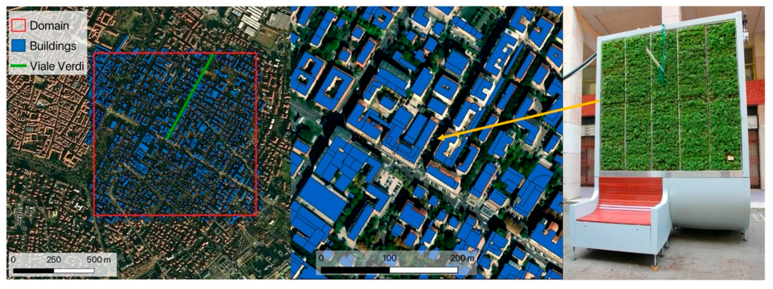
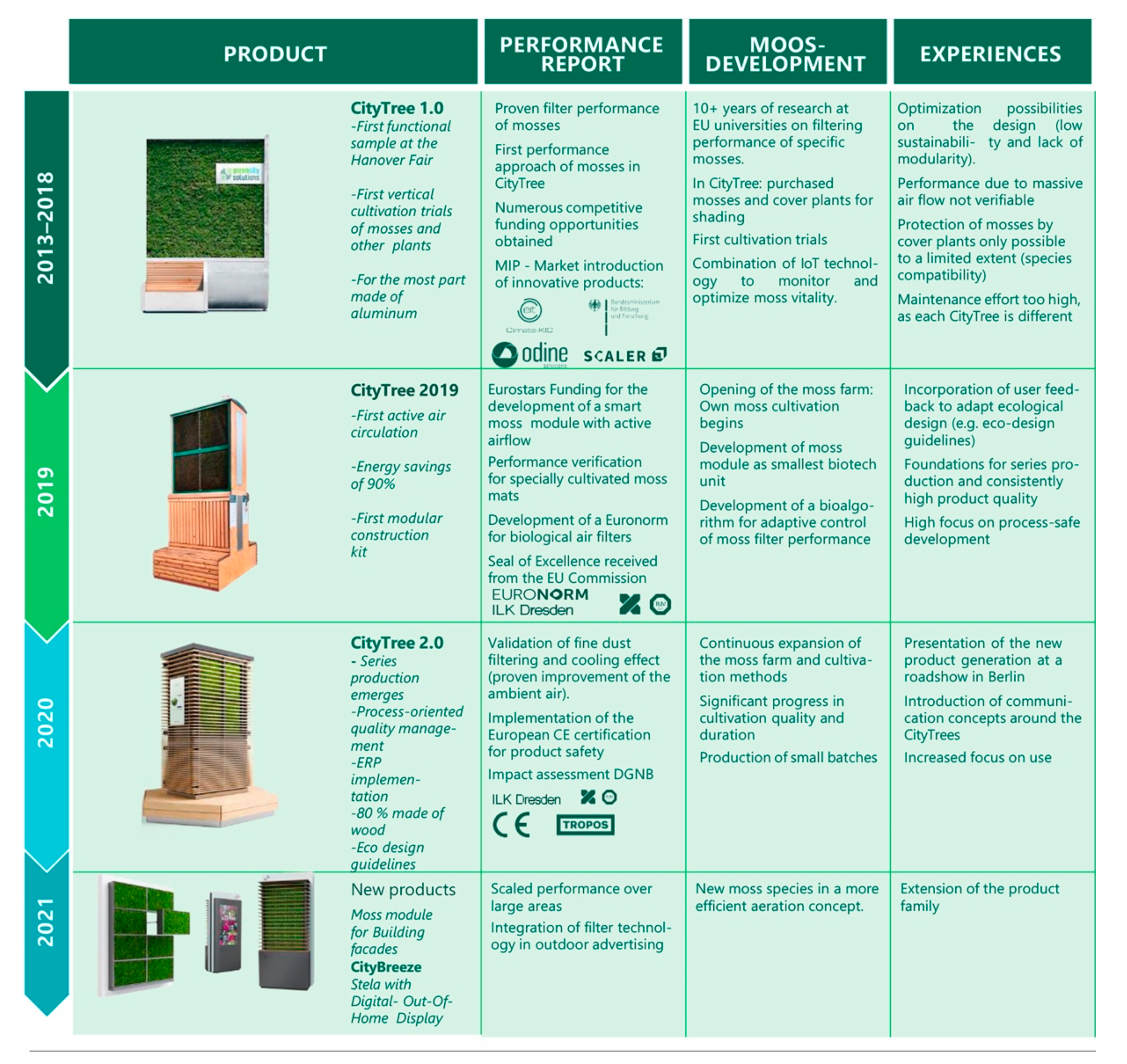
2.1. Green Infrastructure–CityTree Structure

The CT is a 3 × 0.6 × 4 m3 (L × W × H) panel with the two largest vertical sides covered with a combination of hydroponic cultures of mosses and non-vascular plants that act as depositing surfaces for particulate matter and pollutant gases (see [17] for details). The mosses were predominantly Amblystagium varium “Plattenmoos” and Lucobryum Glaucum “Polstermoos” types. The first type was placed in the inner side of the panel since it benefits from reduced sunlight. The second type, better suited for withstanding direct sunlight, was placed on the external part of the panel. Irrigation in CTs is provided by a fully automated system that relies on temperature and relative humidity measurements to ensure the highest efficiency for moss cultures. The newest types of CT host hydroponic cultures of mosses only. Being permeable to air and with their mesh-like texture, mosses can capture atmospheric particulate matter by impaction and deposition when flowed with ambient air. Air flow can be forced in CTs by the internal venting system. As discussed in the companion paper, the “filtration mode” results in enhanced removal of PM but not of NOx with respect to when the venting system is switched off (“passive mode”), most likely due to an increased probability of impact and deposition of solid particles induced by the higher flow rate, not involving the gaseous species [16]. Since filtration requires an energy supply, CTs were operating most of the time in passive mode during the field campaigns in Modena.

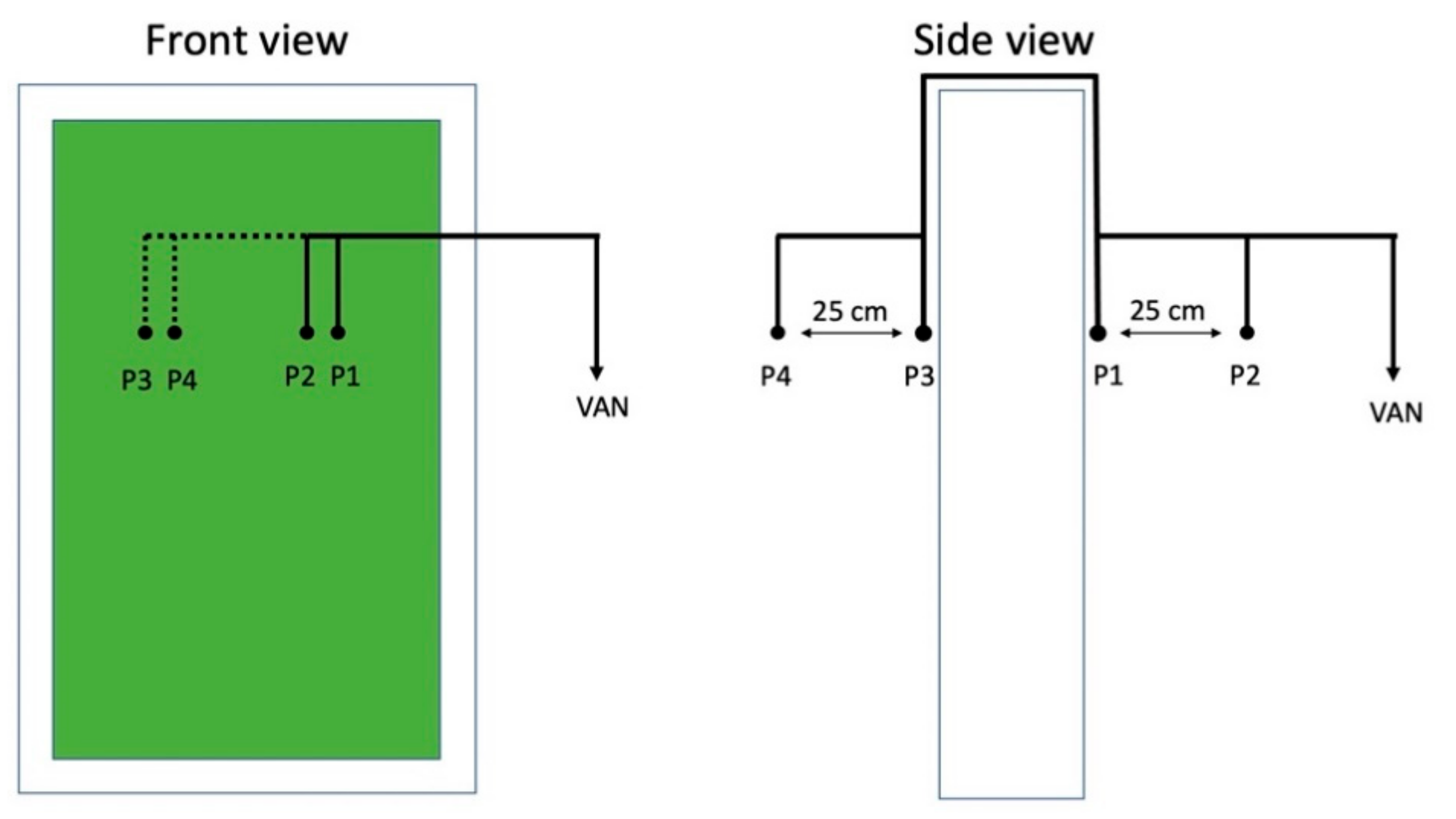
2.2. Experimental Activities

Since 2017, three field campaigns have been performed in order to obtain a complete characterization of the filtration efficiency and deposition velocities of the CT in a real environment, consisting of a urban street canyon, and different meteorological conditions. We considered the western side of the road named viale Verdi (44° 38′ 34.94″ N and 10° 56′ 07.81″ E) in Modena (Italy), (see Figure 1).
In the companion paper [16], data and results from the experimental activities are fully described. For the reader’s convenience, here we report a brief description of the experimental activities. The first measurement campaign was performed between 12 May and 27 June 2017, for a total duration of 37 days. This campaign focused on the determination of the CT deposition velocities for selected air pollutants in spring-summer meteorological conditions. The second measurement campaign was performed from 9 November to 25 November 2017. This campaign aimed at the determination of the CT filtration efficiency when the ventilation system was active.
The last campaign was performed from 27 March to 17 April 2018. The measurements in deposition mode were performed from 6 April to the end of the period for a total duration of 12 days. This campaign focused on studying the removal rates of particulate and gaseous pollutants in winter-spring conditions both in deposition and filtration modes.
The mobile laboratory was equipped with state-of-the-art instrumentation for air quality and meteorological observations. Particle concentrations were measured using a condensation particle counter (CPC, Grimm Aerosol Model 5.403, 1 Hz) for total particle number concentration (PNC) and an optical particle counter (OPC, Grimm 1.109, 31 channels) for particle number size distribution and particle mass size distribution. Both CPC and OPC collected samples with 1 min resolution. The system was able to measure PNC in the range between 0.009 and 1 µm. The OPC was used to measure the particle number size distribution in the size range between 0.25 and 32 µm. The OPC provides estimates of the particulate mass in the PM10, PM2.5 and PM1 size ranges. Gaseous concentrations of NO, NO2, and NOx were measured with a temporal resolution of 1 min. NO, NO2, and NOx were measured using a Teledyne-API (200E analyzer). Black Carbon (BC) was measured by a Thermo Fisher Scientific Multi-Angle Absorption Photometer (MAAP). The instrument provides the atmospheric concentration of the equivalent black carbon (BC) with 1 min time resolution. Furthermore, the mobile laboratory was equipped with a three-dimensional ultrasonic anemometer (R3, Gill Instruments), installed at about 3 m above the ground on a telescopic mast, and a slow response thermo-hygrometer Rotronic MP100A (Campbell Scientific).
Statistically significant passive deposition velocities (first quartile, median, and third quartile of the distribution were provided) for PM10 and NOx, measured during the first and the third field campaigns were used in the PMSS model to evaluate potential reductions of air pollutants concentration in the area nearby the CT. In addition, traffic observations (consisting of vehicle counting) were used to estimate the traffic emission input for the simulation.

2.3. Micro-SWIFT-SPRAY (PMSS)

The modelling system Micro-SWIFT-SPRAY (PMSS) is a suite for simulations of primary pollutant transport and dispersion. PMSS is the parallelized version of the MSS model suite, which is fully described in [29,30,31,32,33,34]. The system is composed of two main model units: PSWIFT, an analytically modified mass consistent interpolator over complex terrain [30], and PSPRAY, a three-dimensional Lagrangian particle dispersion model. The modelling suite can be used for both local scale and microscale simulations, with complex terrain or obstacles such as buildings, which are represented as filled cells in the meteorological field [32,33]. PSWIFT produces mass-consistent wind fields using data from a dispersed meteorological network or from simulated meteorological data at lower resolution.
In PSPRAY the pollutant concentration is simulated by generating a certain number of “virtual” particles, each of them carrying a portion of the pollutant mass. The velocity of the particles is composed by a mean velocity component defined by the local wind computed by PSWIFT, and a stochastic velocity component, characteristic of the atmospheric turbulence. PSPRAY can compute mean and instantaneous concentrations on a three-dimensional grid defined by the user, differentiating the calculation both by “chemical species” and by “source”.
PSPRAY can simulate the dispersion of pollutants from point, area or line sources. The model reproduces the transport, the dispersion and the dry and wet deposition of the airborne chemical species emitted. In particular, PSPRAY is also able to compute dry deposition due to interactions with roofs, walls and ceilings, by inserting species dependent deposition velocities into the model [33].
In its current version and differently from a CFD model [15,53], our model cannot compute the air flow through a porous medium, such as a tree, since the porosity of obstacles has not yet been implemented. However, as already mentioned in the introduction, the bulk deposition coefficients measured in [16] represent a sort of “total deposition” as they include the main effects such as particle interception, absorption and throughflow (see [18]). Moreover, they already take into account the porosity of the vegetation and the complex effects between air motion and vegetation as found in the literature [18,44,45].
In our model simulations, the CT structure was represented as an obstacle with deposition characteristics, which we can parametrize in PMSS. When the filtration mode was activated in the CT, the calculated bulk “effective filtration” deposition velocity was assumed to be the deposition velocity capable of producing the impact of the CT measured in filtration mode. In this way, we could use PMSS to study the spatial characteristics of the filtration efficiency.
As a Lagrangian dispersion model, PSPRAY performs the dispersion of chemical compounds (NOx) in the urban environment. However, chemical reactions occur at this scale, affecting the concentrations of the chemical species [33]. In order to represent this, recent developments have addressed the implementation of several chemical models into PSPRAY (see [33] for more details). However, in the present work, we decided to consider only the dispersion characteristic of the PMSS system, and the chemical models were not implemented.
The PMSS modelling system is a commercial software developed by ARIANET [54]: PSWIFT and PSPRAY codes, in the versions PSWIFT-2.1.1 and PSPRAY-3.7.3, compiled with Intel16 compiler, using OPENMPI library.

2.4. Simulation Set-Up

As mentioned in the introduction, we focused on two-time frames: 12–31 May 2017; and 5–17 April 2018. In these time frames the CNR experimental campaigns provided a complete characterization of the bulk deposition velocities for NOx and PM10. Since these measurements did not show a significant variation during the campaigns, their average values were used for the simulations. Only for the PM10 concentrations was the filtration efficiency retrieved of the CT operating in active mode. The reason for selecting PM10 lies in the fact that [16] reported neglectable abatement for the NOx concentrations when the CT operated in active mode.
We performed two sets of simulations:
1.
For the year 2017, we ran PMSS to simulate vertical deposition due to the CT operating in passive mode (only deposition).
2.
For the year 2018 we reproduced the air pollution abatement linked to the deposition vertical velocities when the CT operated in passive mode (as in 2017). In addition, we studied the PM10 concentration abatement produced when the CT filtration mode was activated. Here we used the passive deposition velocity, calculated from measurements analysis, able to produce the same pollutant deposition measured with the CT in filtration mode (see [16]).

2.4.1. Input Meteorological Data

Meteorological data used to feed the diagnostic model PSWIFT for 2017 and 2018 periods were provided by RAMS (Regional Atmospheric Modelling System, [55]), the meteorological model driving the national Air Quality modelling system MINNI [56,57,58] and the air quality forecast system FORAIR-IT [59,60].
Hourly data of meteorological fields were used by PSWIFT to reconstruct the three-dimensional wind, temperature and turbulent flow at 2 m resolution.
The meteorological parameters that are used in the model (such as relative humidity and precipitation) affect only the state of the atmosphere and cannot change the deposition characteristics of the CT, which are described by the bulk deposition velocity that is constant for each pollutant.

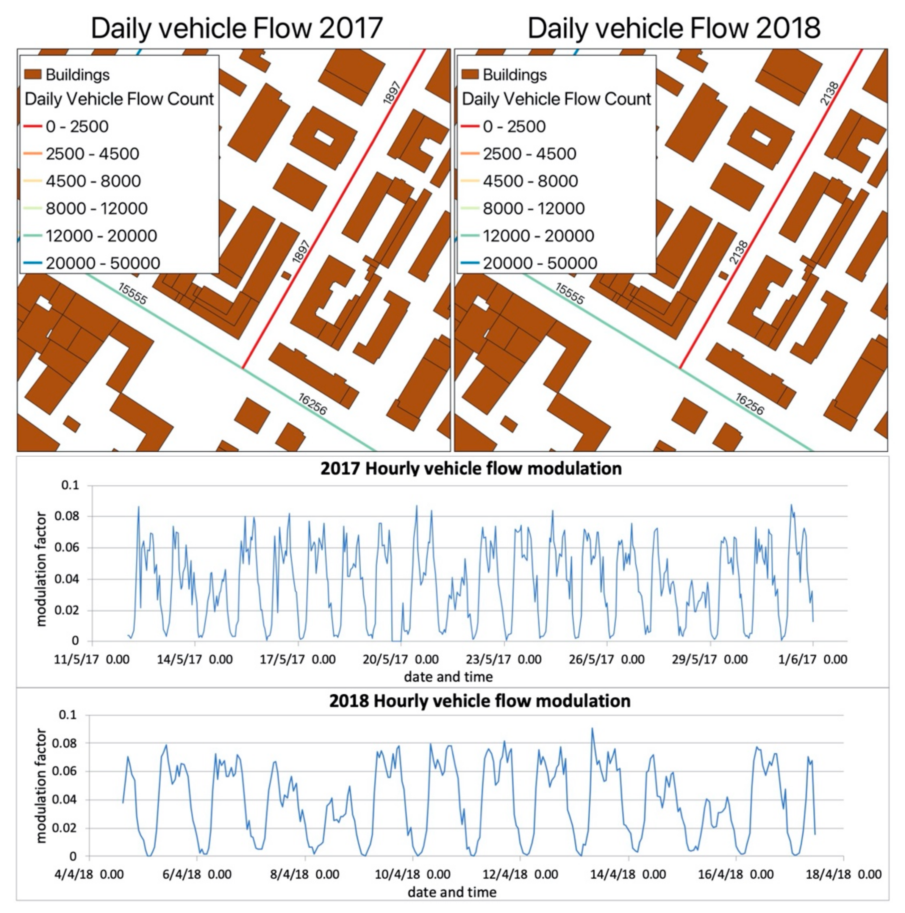
2.4.2. Simulation Domain, Area and Obstacles

We set a 1 × 1 km2 horizontal domain that was centered in viale Verdi, where the CT was located (Figure 1). The domain is shown by the red square in Figure 1 and covered an adequate fraction of the emissions of the city while providing that the CT unit was far enough from the domain border, where the model uncertainty is generally higher. The spatial resolution of 2 m was chosen to ensure that the model represented the CT as closely as possible while keeping computational time within acceptable values. For the vertical grid, we chose the following 25 levels above the ground: 0, 1.5 m, 3 m, 4 m, 6 m, 8 m, 10 m, 13 m, 16 m, 19 m, 22 m, 25 m, 30 m, 35 m, 42 m, 50 m, 60 m, 80 m, 120 m, 160 m, 200 m, 240 m, 300 m, 380 m, and 700 m. Since buildings are represented by the model as filled cells in the computational grid, vertical levels were chosen in order to properly describe the range of the heights of the buildings within the domain.
As mentioned in the introduction, in our simulations the CT was represented as an obstacle with deposition characteristics. This is a sound assumption, as [44] showed that, rather than representing every leaf, air flow and particle-leaf interactions are represented statistically by using a continuum approach. As for the case of the CT that contains a sufficiently large number of single vegetated elements, the effects of individual vegetated items are irrelevant in the average transport through the volume. Moreover, each vegetation item of the CT surfaces has dimensions much smaller than our model grid size. On this basis, we represented the CT as a barrier with proper measurable parameters describing vegetation (see for example [44,45]), which are fully provided in our modelling study by the measurement campaigns of [16].

2.4.3. Bulk Deposition Velocities for PM10 and NOx

The bulk deposition velocities used in our simulations are of two kinds:
  • Bulk Deposition Velocities with the CT in passive mode (filtration switched off)
We considered the main statistical parameters of deposition velocities resulting from the measurements of both the 2017 and 2018 campaigns. Upon observing that the values did not change significantly, the results from both campaigns were included for a more robust statistic.
Measurements of air pollutants were performed, alternatively, through a computer-controlled valve switching system, at two different horizontal distances on both sides of the CT (at the front and at the rear of the wall). Figure 2 shows the sampling system that was composed of four identical conductive silicon sampling tubes connected to a common inlet through four electronic valves for automatically switching the inlet (P1, P2, P3 and P4) every 7 min, resulting in a complete cycle of 28 min. Inlet P1 and P2 were positioned in proximity (at 5 and 30 cm respectively) of the surface of moss and leaves on the roadside of the CT panel. Inlet P3 and P4 were in a specular position on the curb side of the CT panel.
The statistical parameters considered for the estimate of the deposition velocity were the first quartile, the median and the third quartile, and are presented in Table 1. These values are consistent with the deposition velocity values found in the literature [61].
  • Bulk Deposition Velocities for PM10 with the CT in filtration mode
The filtration mechanism occurs in the CT by means of fans operating inside the structure, and it is a more efficient mechanism than the passive deposition (e.g., [16,62,63]). In particular, [16] showed that the aerosol removal efficiency of the CT was from ~3 to almost 20 times higher in filtration than in deposition mode.
We provided an estimate of the effect of the CT in filtration mode on particulate matter concentrations to study its influence at increasing distance from the structure. Considering PM10 measured concentrations, CNR and Consorzio PROAMBIENTE calculated an “equivalent deposition velocity” as the bulk deposition velocity that the CT should have in order to produce the observed pollutant reduction in the active filtration mode. The average value of about 0.024 m/s was obtained and is consistent with the largest values of deposition velocity intervals found in the literature.

2.4.4. Emissions

We computed the traffic emissions in viale Verdi from the hourly vehicle flows measured during the campaigns from 12–31 May 2017 and from 5–17 April 2018. Hourly modulations of buses passages were calculated according to the public transportation timetable at the bus stop. In all the other roads of the simulation domain, total daily vehicle flows generated by a flow assignment model run for 2017 by the Municipality, combined with hourly traffic modulation measured in viale Verdi, were used (e.g., Figure 3).
The composition of the vehicle fleet, in terms of age, emission standard, displacement, and fuel, was retrieved from the public registry of motor vehicles for the year 2017 (which was the latest published online at the time of the study) and for the city of Modena. The emission input for PSPRAY has been calculated by TREFIC (Traffic Emission Factors Improved Calculation), a software designed by ARIANET [64] for the calculation of road emissions. TREFIC calculates emission factors (EFs) using the COPERT 4 methodology [65], based on vehicle type, fuel consumption, average travelling speed and road type.

2.4.5. Parallel Run Details CRESCO

PMSS allows for parallelization in time for PSWIFT and for PSPRAY, both with respect to the domain, referring to a multi tiles domain, and to sources/particles decomposition [31]. Our domain is an area of 1 × 1 km2 at the resolution of 2 × 2 m2, which is suited to be represented by a single tile [32]. Therefore, our PSPRAY simulations were handled by a single tile of 501 × 501 cells, and the computation was parallelized with respect to particles.
We conducted the simulations on the CRESCO/ENEAGRID High Performance Computing infrastructure funded by ENEA [52]. As the model system was structured, each 12-day-simulation consisted of 12 single model runs, each simulating 24 h. The restart option was applied, i.e., for each simulated day the values of the pollutant concentrations calculated for the last hour were saved and used as initial condition for the following run.
The simulation duration depends also on the number of emitted particles and on the concentration resolution required. In our simulations, the total number of emitted particles reached peaks of about 34.3 million particles per day, with a typical particle number per time step of 4000. Here we used 264 cores and for PSPRAY, which represents the most CPU demanding part of the system, the CPU time per core per simulated day was 470 s. A summary of the whole simulation set-up is provided in Table 1.

2.4.6. NOx and PM10 Reduction Operated by the CT

In order to quantify the abatement due to the presence of the CT on PM10 and NOx concentrations, we set up two simulations for each mode (deposition for 2017 and 2018, and filtration-like mode for 2018) that were equivalent to considering the cases with and without the CT. In particular, we considered the measured deposition properties of the CT as an on and off parameter in the model runs, similarly to what was done in the study [46]. Then, we calculated the percentage difference of the PM10 and NOx concentrations with and without the deposition on the CT as metrics of its impact on the air quality.

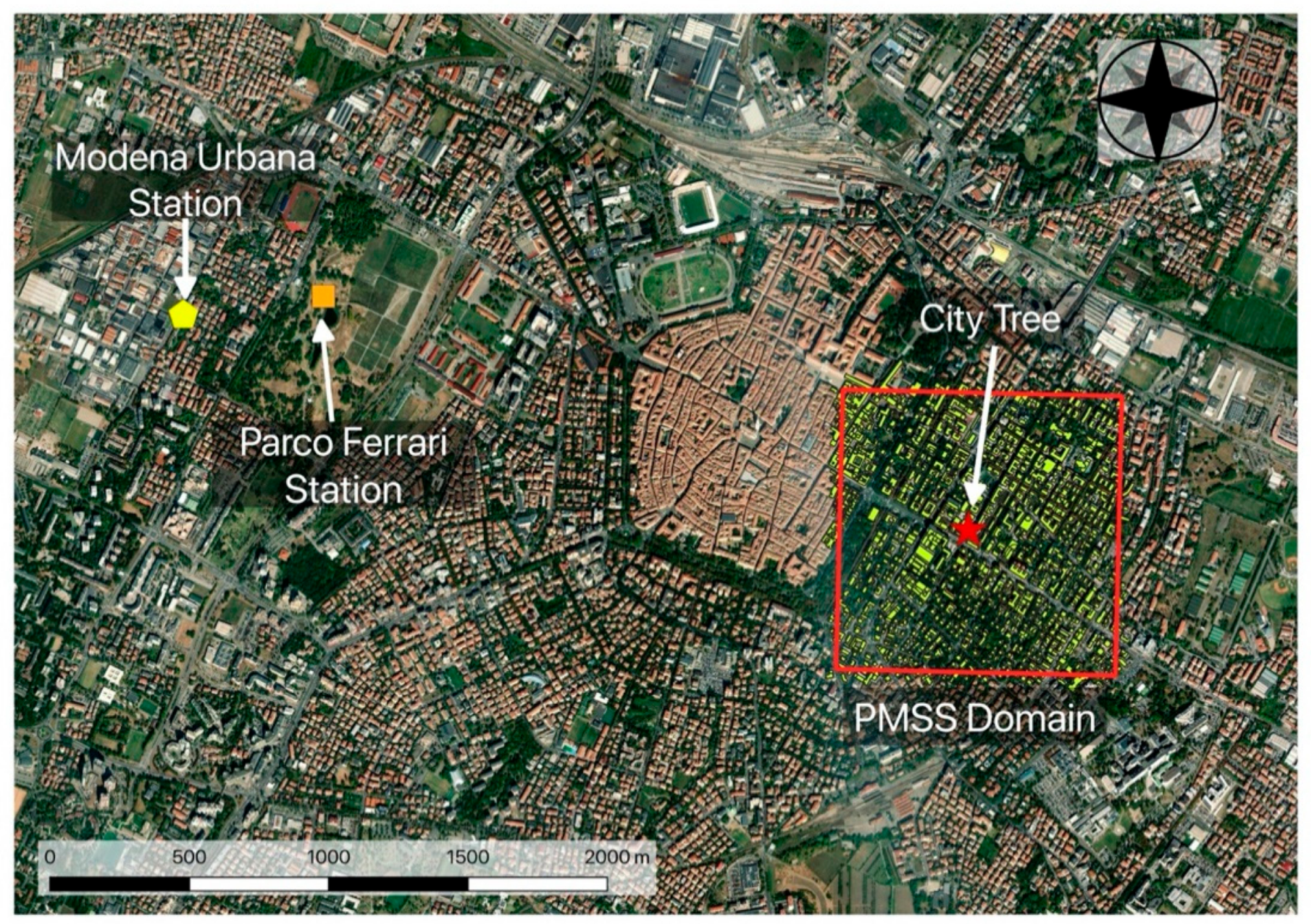
2.5. Reference Air Quality and Meteorological Data

The model validation represents a key factor to evaluate the model performances, and thus to assess the reliability of the results. Since our simulation took into account only primary emissions, to analyze how well our model reproduces NOx concentrations, we needed to estimate the secondary contribution due to atmospheric chemicals processes. Our best indicator available for secondary contribution to NOx concentrations were the measurements of urban background NO2 concentrations, consisting of NO2 hourly concentrations measured in the air quality station of Parco Ferrari (10° 54′ 22.8″ Lon, 44° 39′ 2.2″ Lat, 34 m a.s.l (see [66]).
Concerning the meteorological data, we used wind speed and direction data measured by ARPAE station located in (10° 55′ lon, 44° 39′ lat, 35 m altitude a.s.l.). Both stations are presented in Figure 4.

2.6. Tools for the Analyses

For the analyses performed, we used the FAIRMODE IDL-based DELTA software tool version 5.4 [67,68] provided by the Forum for Air Quality Modelling in Europe [67], and R-cran based scripts [69,70].

3. Results

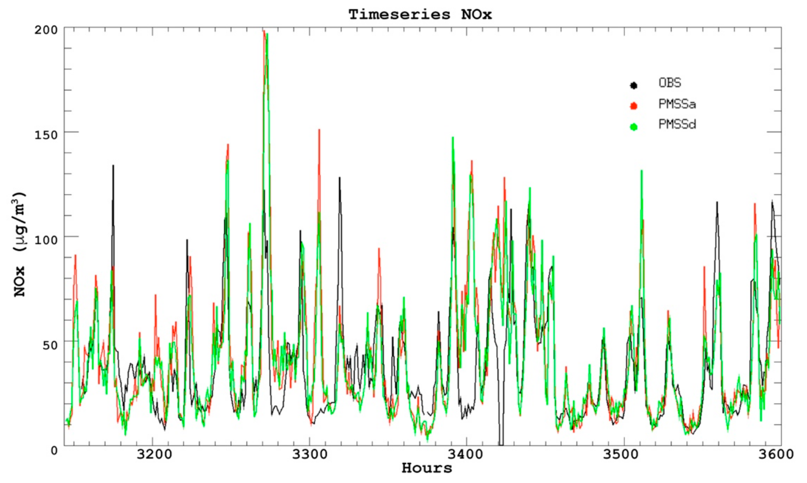
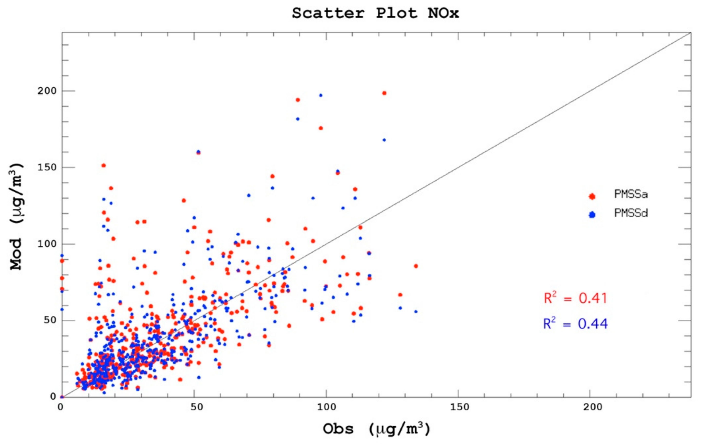
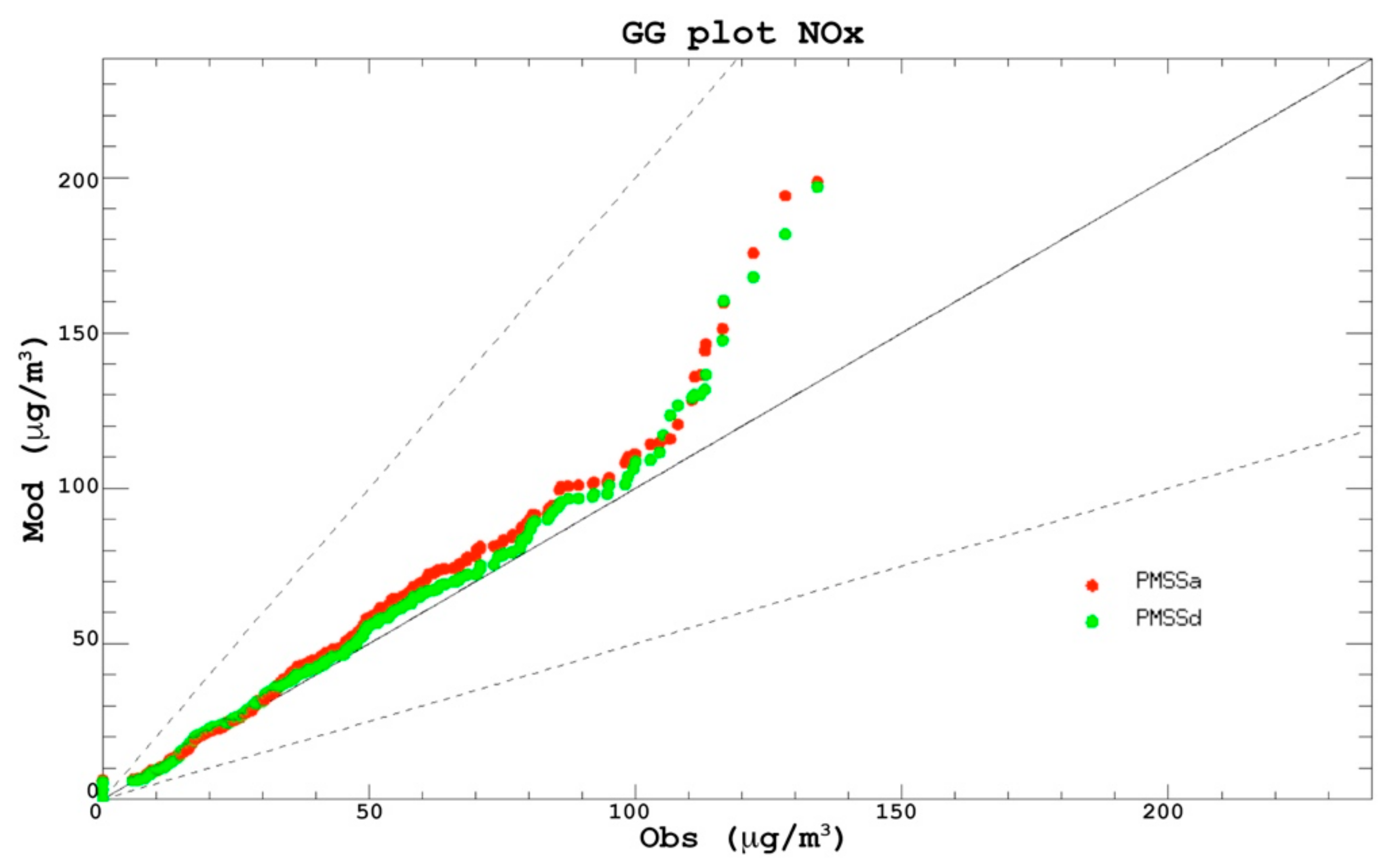
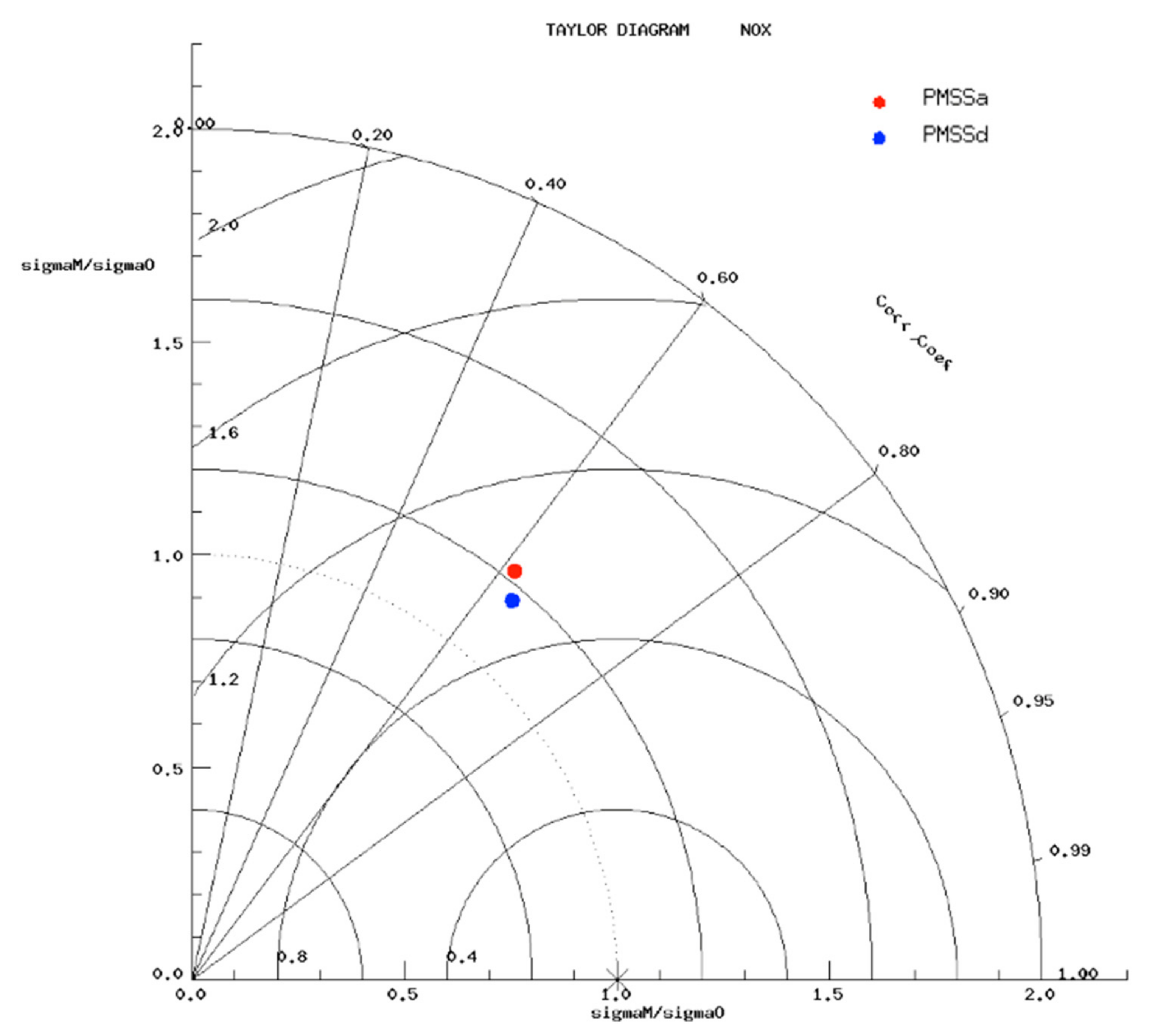
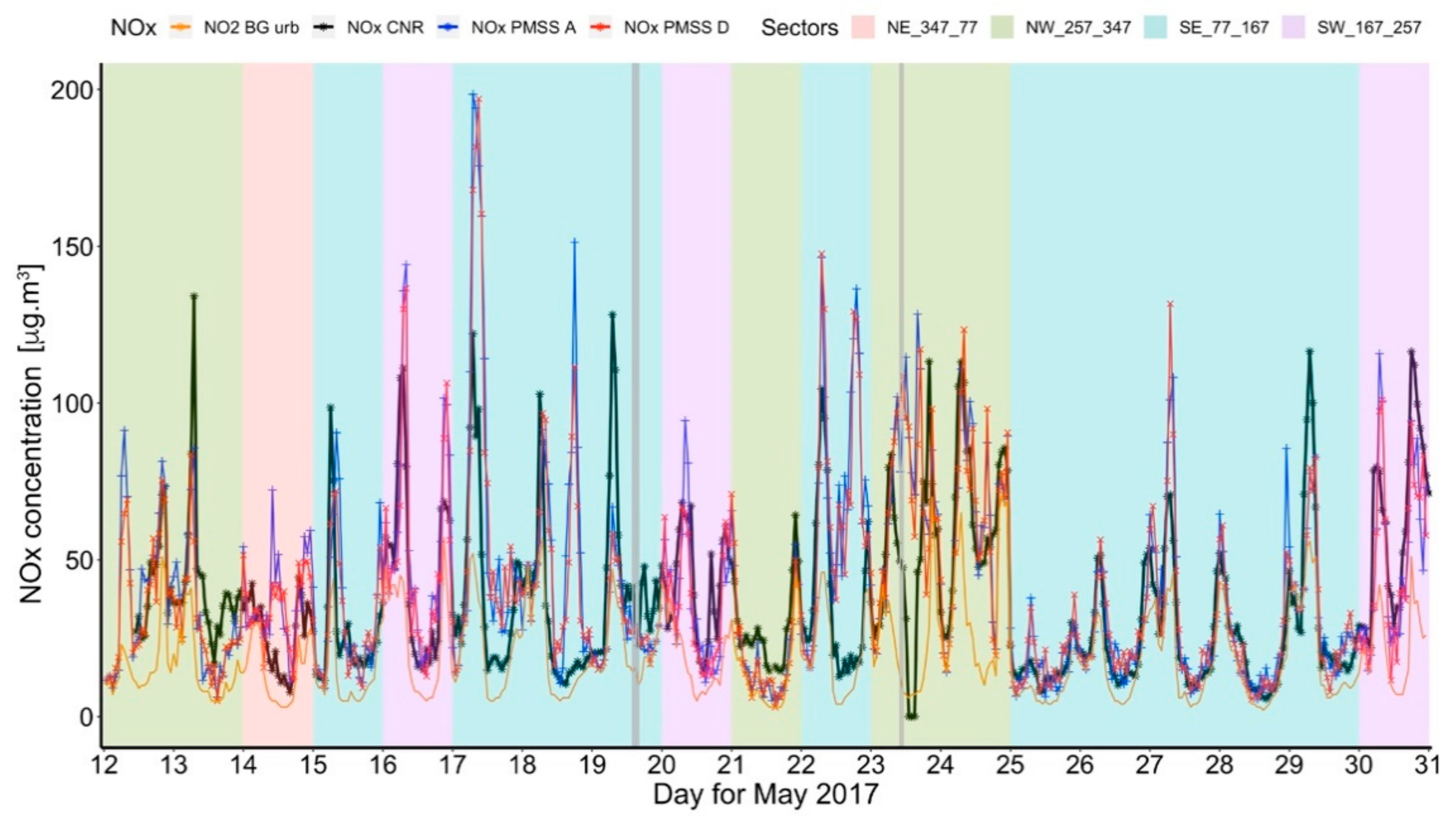
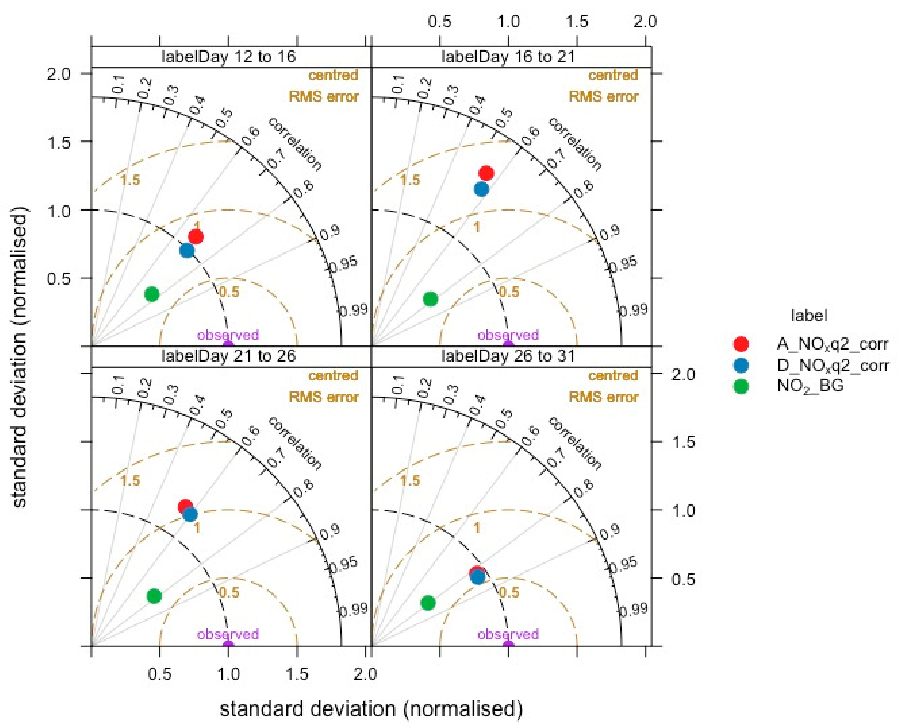
3.1. NOx Modelled and Measured Data Evaluation

To evaluate the PMSS performances, we studied the NOx concentration time series for the year 2017. We focused on this time period since the measurement campaign from 12 May to 27 June 2017 was the longest (37 days). We compared hourly NOx concentrations measured during the CNR campaign with the simulated NOx after adding the background concentrations. The reason for choosing the pollutant NOx relies on the fact that we used our PMSS modelling system studying the dispersion of pollutants, neglecting chemical reactions (see Section 2.3). Therefore, it was possible to properly represent air pollutions from primary sources only. In our case, the NOx concentration is produced mostly by traffic, thus the approximation that is made neglecting the chemistry has a smaller influence on the simulated concentration that can be corrected by adding a background concentration, which represents most of the secondary contribution.
Hourly measurements of NO2, provided by the urban background air quality station located in Parco Ferrari (see Section 2.5), at a distance of about 2 km from viale Verdi, were used as background concentration values, since data for the concentrations of NO and NOx were not available at this station.
In Appendix A we present detailed analyses to assess our model performances.

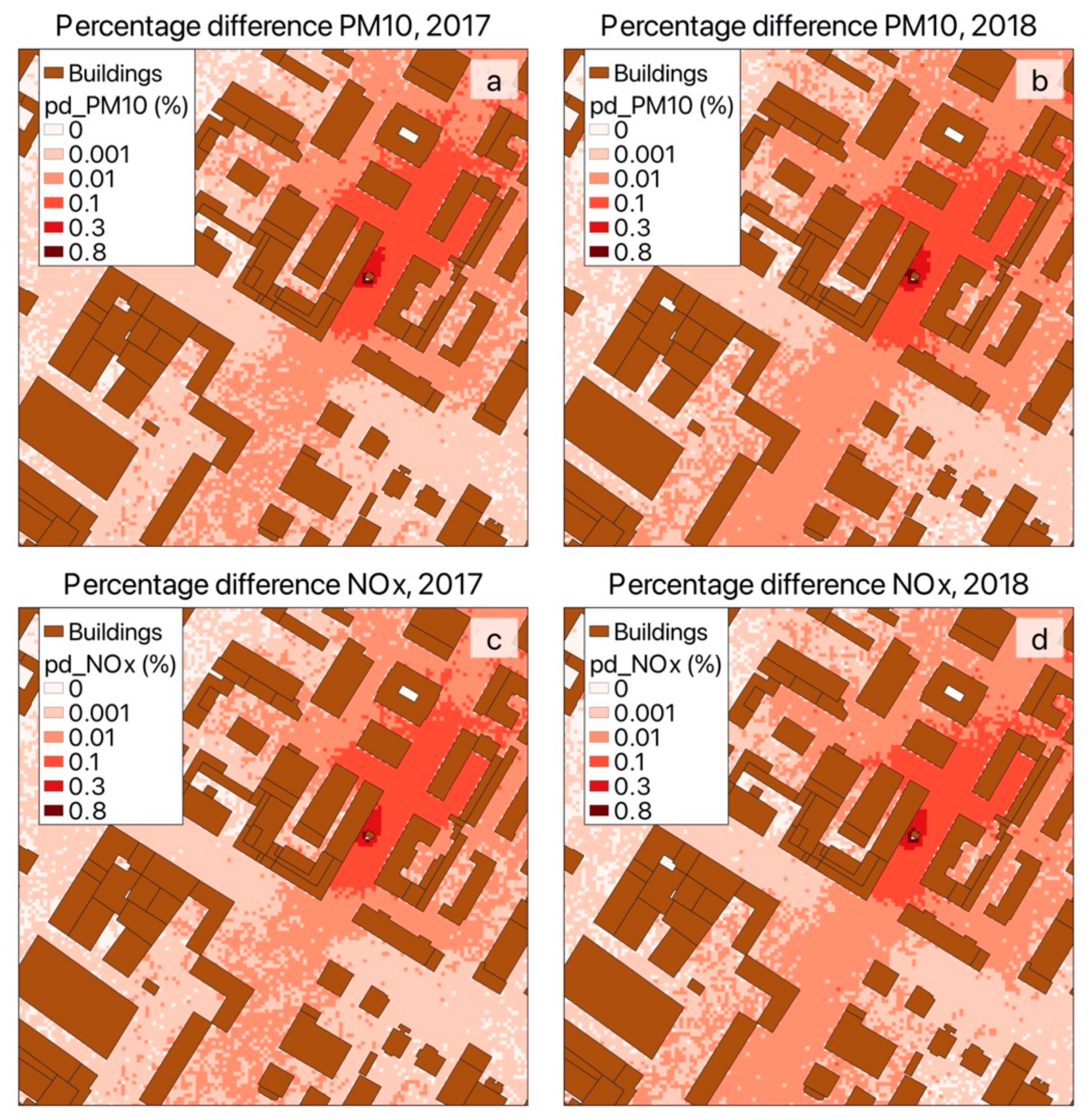
3.2. Green Infrastructure Abatement

The results of the simulations are presented here as averages over the two simulation periods (19 days for 2017 and 12 days for 2018), in order to show the pattern of the area interested by the effect of the presence of the CT.
Here the differences between the simulations with and without the CT are presented as mean PM10 and NOx percentage concentration differences. All the graphics reported show results using the median of the measured deposition velocities. Similar maps corresponding to the values obtained using the first and third quartile of the deposition velocity distributions for each case simulated did not differ significantly, therefore they are not shown.

3.2.1. CT in Passive Mode-Deposition

Median values of the deposition velocities were 0.0012 m/s and 0.0011 m/s for PM10 and NOx, respectively (see Table 1).
From Figure 5, the effect of the CT in passive mode (deposition) translates into a maximum concentration reduction of about 0.8% for both PM10 and NOx concentrations. Though our simulations are not directly comparable to the CFD simulations in the TNO study, nevertheless our results for PM10 are in agreement with those found in Amsterdam [46]. For a given deposition velocity, we can define a “region of influence” of the CT as the area where the concentration reductions are larger than 10% of the maximum value reached. For the CT operating in passive mode, the region of influence has concentration reductions larger than 0.1%, and it is found in proximity to the CT, with an extension of about 10 × 20 m2 more or less centered on the CT position, as shown in Figure 6.
Figure 6 also indicates the location of the two points (Figure A1), A and D, in which we studied the NOx concentration comparisons with measurements (presented in detail in Appendix A) and in which we extracted the vertical profiles shown in Figure 7 and Figure 8.

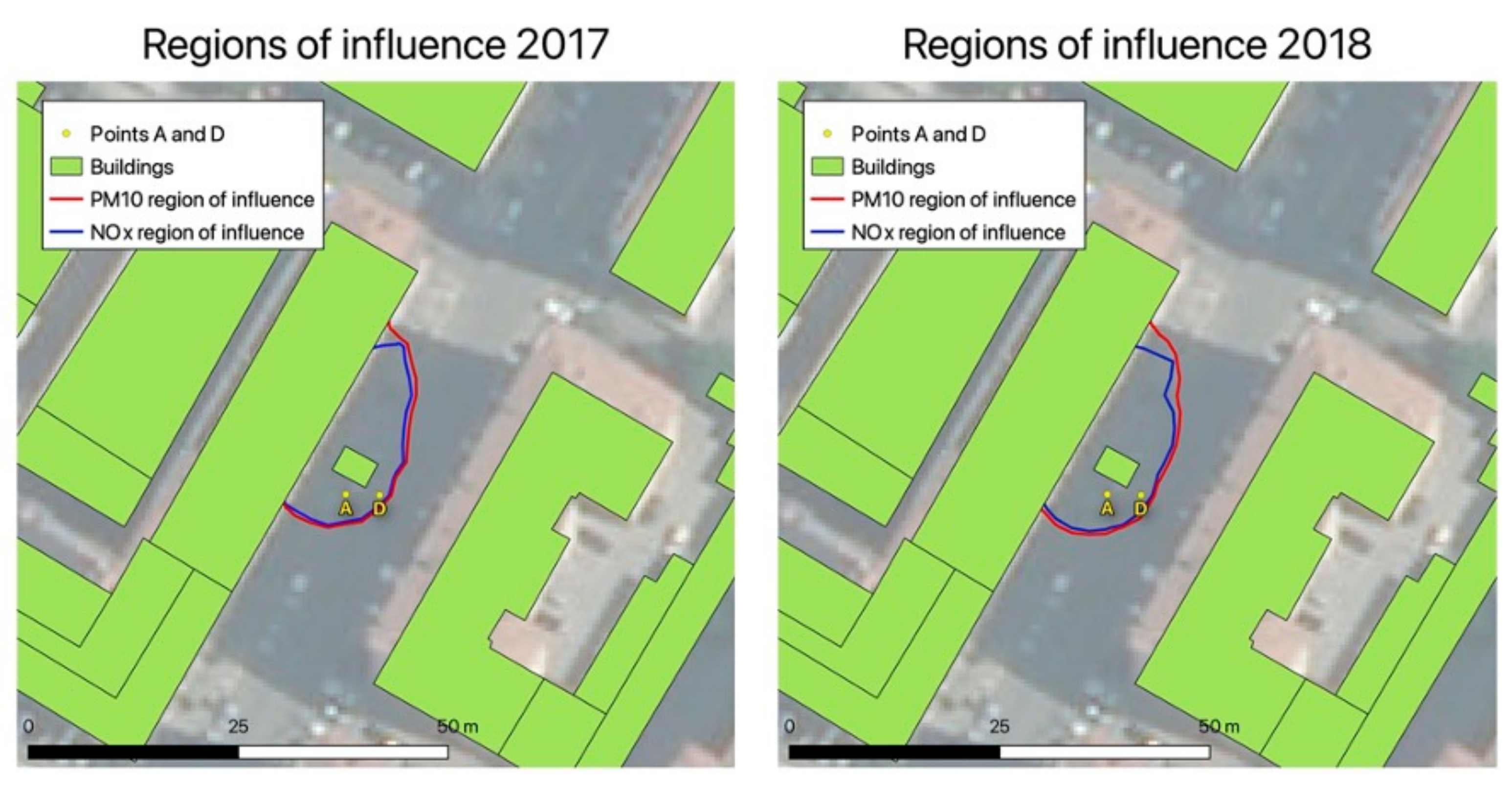
3.2.2. Vertical Profiles of Pollution Reduction in Passive Mode

The mean vertical profiles for the pollutant reduction are reported in Figure 7. In particular, we took into consideration two points, A and D, which were close (point A) and 4 m away (point D) from the structure (see Figure A1).
We observe:
  • Reduction profiles for PM10 and NOx have the same characteristics. They have the maximum reduction values in the first few meters above the ground. The reduction decreases significantly at heights above the green infrastructure (above 6 m).
  • For both NOx and PM10, the maximum pollutant reduction is obtained very close to the green infrastructure, at point A, with values of about 0.5%. At point D, the maximum pollutant reduction decreases to 0.1–0.2%.
  • Air pollutant reduction decreases rapidly, moving away from the green infrastructure, both in the vertical and in the horizontal directions.

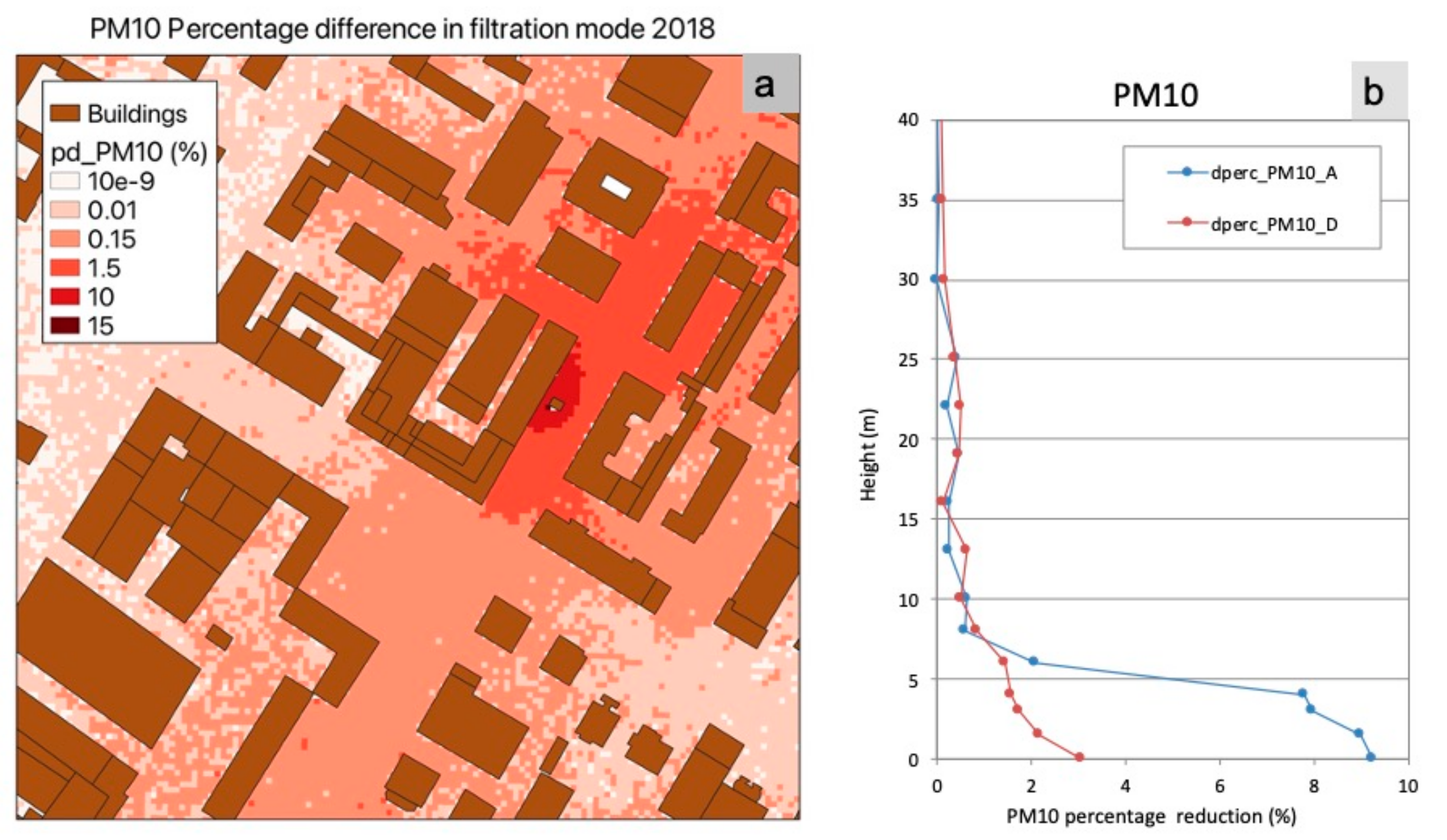
3.2.3. CT in Active Mode (Filtration) for PM10 Concentrations in 2018

The results for the CT in active mode of operation (filtration) for PM10 concentrations in 2018 are shown in Figure 8.
The space distribution of the impact did not significantly change with respect to the previous simulations with lower deposition velocities (here the value is 0.024 m/s, instead of about 0.001 m/s). However, the values of the maximum PM10 concentration reduction increased to 15% very close to the CT. In analogy with CT in passive mode (deposition) cases, we observe a very similar region of influence with different values and largest concentration reductions at the southwest CT corner. Here, in the areas where the percentage difference is higher than 1.5%, we observe a much larger extension covering most of viale Verdi and some of the lateral roads (approximately 10 × 30 m2). The vertical distribution of the impact of the CT (Figure 8b) has not significantly changed with respect to the passive deposition case (Figure 7).

4. Discussion

When we take into consideration the pollutant abatement caused by the CT in passive mode (deposition), we observe that reductions of NOx and PM10 concentrations are smaller than 1% in an area of about of 10 × 20 m2 around the CT and at the same height as that of the green wall. Comparing our results to those obtained in other studies is not an easy task. The only other modelling study published on a similar CT as that deployed in Modena, was performed by TNO [46]. The simulations in this study were performed by considering a realistic situation using factory specifications for the CT, therefore not considering input measurements for the model, as done in the study presented here. Although our modelling results are not directly comparable to those of the TNO study, nevertheless our results for PM10 in the case of passive mode of operation are in agreement with those found by TNO [46].
When the CT operated in active mode (filtration), our modelling estimate of the impact suggests pollutant reductions of a larger order of magnitude, reaching values of about 15%. As for the previous result, in this case finding similar results in the literature for comparison was not an easy task. A recent study [71] involving a similar type of green wall with filtering capabilities placed at the edge of a highway showed measurements that can be compared to the filtration efficiency measured during the CNR campaigns. These measurements are in some agreement, in the experimental estimate of the filtration efficiency for PM2.5, with the results of the CT experimental campaigns [16].
We observed that the region of influence has about the same shape and dimensions for both 2017 and 2018, with the CT in passive mode, as well as for the case with the CT in active mode of operation. Given the differences in the setups for the 2017 and 2018 simulations, especially regarding emissions and meteorological conditions, we expect that this area is more significantly influenced by the building pattern and distribution than by CT position in relation to the buildings. Indeed, in preliminary studies conducted for the year 2017, with the same setup with the exception of the CT position, the area of influence showed a shape which did not significantly differ from the one here presented in terms of contours, size and pollutants abatement.
We can conclude that a single CT will not have a significant impact in the reduction of particulate matter and nitrogen oxide concentrations in the whole urban extension. This finding is consistent with the work of [46] where several hypothetical configurations were analysed, including set ups with many CT structures. When more units of CT were represented, [46] obtained pollutant removal in the area considered was less than 20–30%. However, when looking at air pollution in hotspots and/or considering specific building arrangements, these abatements could be achieved.
In the present work, the reliability of the simulated reduction operated by the CT depends on the quality of our model simulations, e.g., we assumed that our model could represent absolute concentrations well, given our specific traffic primary emissions as input. The analyses of the measured and observed NOx concentrations in Appendix A aim to investigate the soundness of our results. The validation of a pollutant such as particulate matter is more complex, not having considered as input all the precursors of the PM secondary components, nor the chemical reactions in the atmosphere that generate these components.
In Appendix A.2, we observed that the values of the NO2 background concentrations were generally close to 20 μg/m3, and they were associated with prevailing easterly winds (up to 6 m/s). These concentration values were possibly generated by air being transported from Modena city center that, due to strict traffic regulations, is less affected by traffic than peripheral areas of the city. Differently, larger NO2 background concentrations (above 50 μg/m3) were measured with SW-SE winds of less than 3 m/s, and they were possibly brought from major traffic roads located southward, some kilometers away from Parco Ferrari.
The NOx observed and modelled concentration analyses reported an overall good agreement (see Figure A4, Figure A5, Figure A6 and Figure A7). The modelled values are generally close to the observations (see Figure A4). However, in specific cases the simulated concentrations are higher than the measurements (Figure A5 and Figure A6). In particular, the measured and modelled hourly data show a dispersion that changes with the concentration values: for concentrations of less than 50 μg/m3, the two distributions are very similarly normally distributed (e.g., Figure A6), while for higher values (specifically for more than 100 μg/m3) the model tends to overpredict the NOx concentrations.
To further investigate the comparisons of the NOx concentrations, we took into account groups of days (Figure A9) and local and urban wind directions classified according to four sectors (Figure A10 and Figure A11) (Appendix A.1). We found that:
  • Wind measurements taken at the urban scale (at Modena Urbana) and close to the CT (CNR measurements inside the urban canyon) are significantly “decoupled” as already well documented in the literature (e.g., [72]). It was very difficult to establish a relation between the urban and local wind datasets, likely to be due to the air circulation specific to the street.
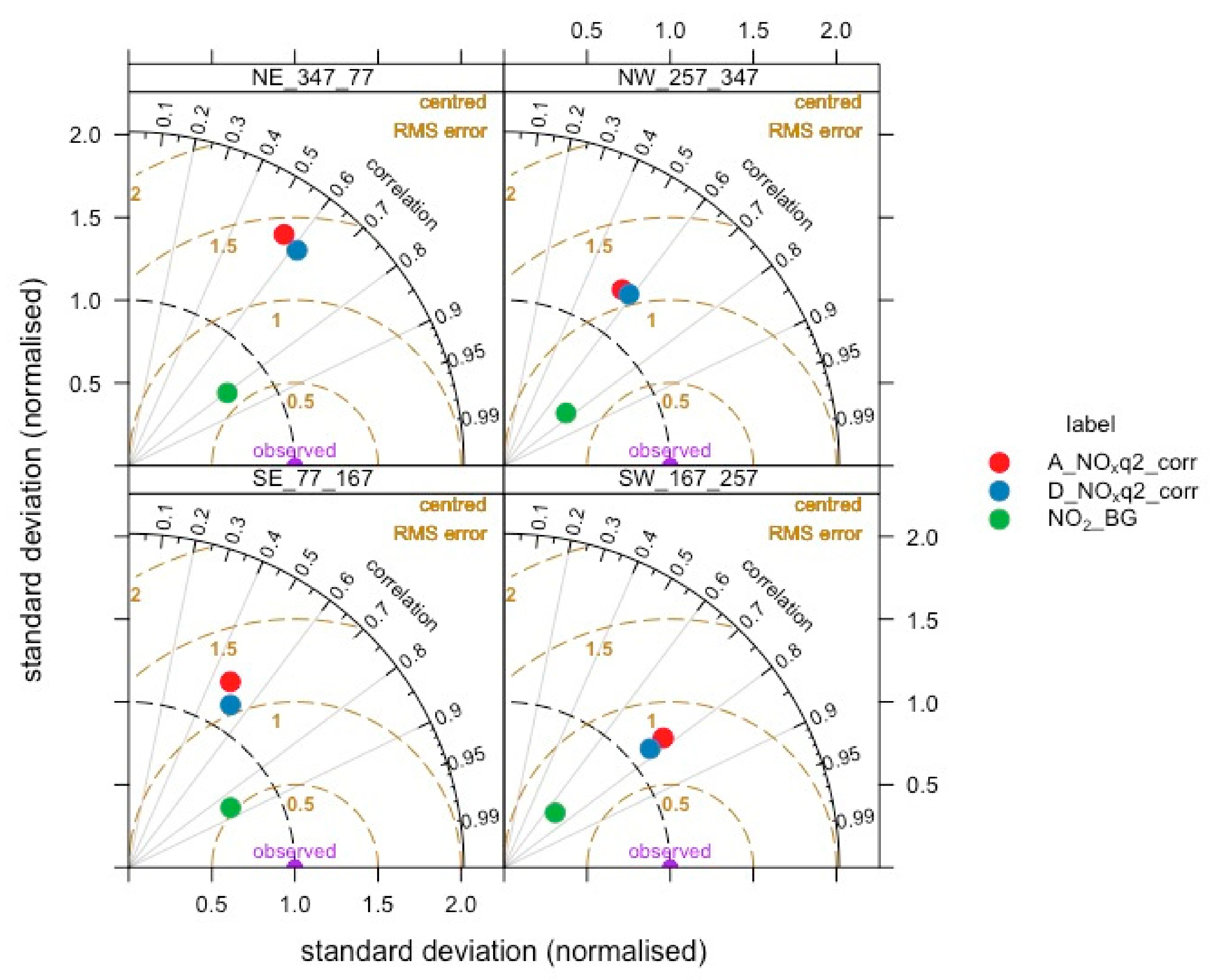
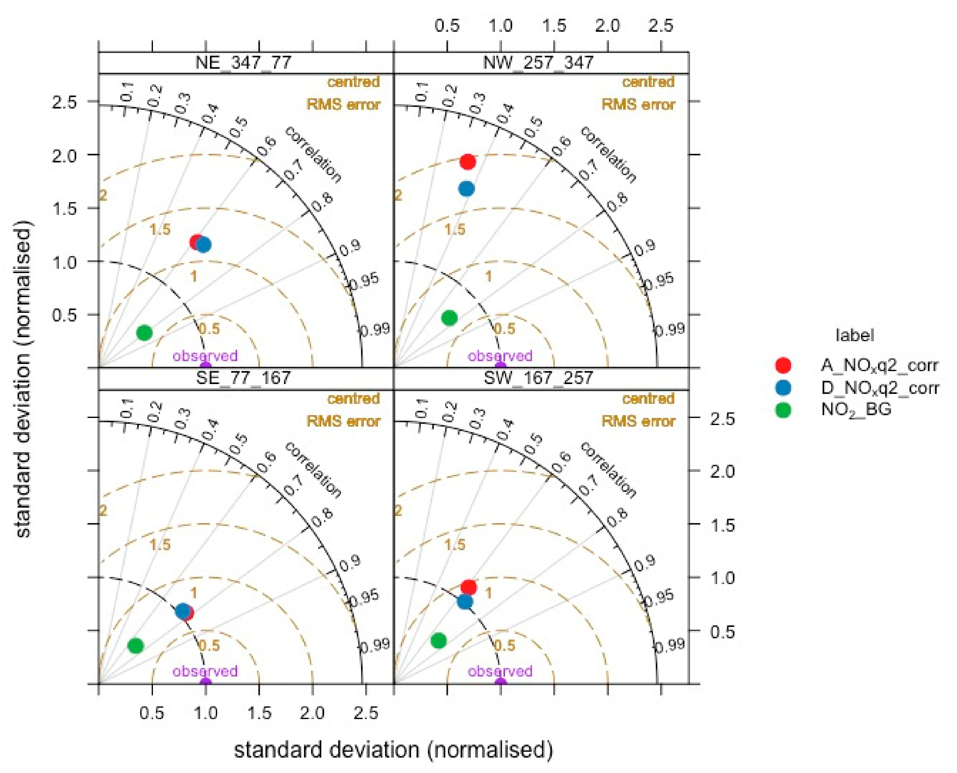
  • The agreement between modelled and measured data is significantly more evident during the days 25–31 May, characterized by urban south-easterly wind and NOx concentrations between 20–100 μg/m3. During the days 26–31 May, the Taylor diagram shows the best agreement with correlation values of about 0.85 and normalized standard deviations close to one.
In the previous settings, to assess if the NOx concentration distributions would spatially differ close to the CT, we analysed the concentrations at the points A and D (see Appendix A.1). However, we concluded that the distributions at the two locations did not differ significantly (e.g., we obtained similar statistical scores for both A and D, from the Taylor diagrams).
We did not identify the reasons for the good agreement obtained during 26–31 May. In addition, we need to further investigate the reasons why our model tends to overpredict NOx concentrations higher than 100 μg/m3.
Note that the NO2 background concentration measurements did show a very good correlation with the CNR local measurements. This represented a key factor for the overall good agreements between measured and simulated NOx concentrations at the local scale.

5. Conclusions

We presented an application of the modelling suite Micro-SWIFT-SPRAY (PMSS) as a reasonable tool for an estimate of the impact of a single CityTree (CT) on the abatement of air pollution concentrations, such as PM10 and NOx, in viale Verdi, Modena (Italy).
We applied the Lagrangian model Spray considering:
  • The specific urban setting centered in viale Verdi, Modena (obstacles and buildings);
  • A prescribed location of the CT consistent with the experimental field CT installation;
  • Meteorological data and emission features coherent with the first and the third research campaigns;
  • Values of bulk deposition velocities deriving from the experimental campaigns (and in agreement with results obtained in the literature).
PMSS simulations showed that the passive operational mode of the CT may produce air pollutant concentrations abatement larger than 0.1% and up to about 0.8% in an area of 10 × 20 m2 around the CT and along the vertical extension of the green infrastructure (4 m). The area may depend on the urban infrastructures design.
When the CT operated in filtration mode, by using a value of bulk deposition that produced the same PM10 concentration abatement, in terms of concentration difference between the values measured in front and at the rear of the panel, we obtained a PM10 concentration reduction of about 15% close to the CT. This is the best estimate of the active CT mode operation on PM10 concentration abatement achievable with the PMSS suite. Furthermore, this finding suggests that active filtration mode can abate particulate matter concentrations at least one order of magnitude more efficiently with respect to the only deposition removal and that the abatement is present along the entire vertical extension of the CT.
The novelty of our results lies in the use of measured passive deposition velocities during three intensive field campaigns in the city of Modena (Italy) [16]. In addition, an assessment of model performance was developed with reference to NOx modelled and measured concentrations. For the year 2017, good agreement resulted between observations and modelled data reporting overall correlation indexes of about 0.6 and normalized standard deviations of about 1.25.
The results of the present study indicate that a single CT will not have a significant impact in improving the air quality of a street along its full length. These findings, tested with different meteorological conditions and different emissions input for the experimental time periods in 2017 and 2018, show that, according to the value of the deposition velocity, the major reduction effect occurs in a specific area in the neighborhood of the infrastructure (the “region of influence”) in both deposition and filtration modes. Therefore, an effect in reducing particulate matter and nitrogen oxides concentrations, and thus population exposure, can still be achieved for specific environments (e.g., sidewalk benches, small gathering areas, bus stops, school or hospital entrances).
On the basis of these results, we expect that a cluster of CT modules, properly located in an urban context, could design restricted densely populated areas with consistent air pollution reduction, the so-called “clean air zones”, where citizens are expected to spend time during rush hours. For practical applications, parameters such as energy and water consumption per operating hour are important. Such technical parameters of CTs were not optimized at the time of our field campaigns, while later generation CTs have been accurately engineered to account for power and water supply. A comparison of the technical features of the new CT model with respect to the one deployed in Modena (a CT 1.0 version) is available in Appendix B (Figure A12). In new CT 2.0 models, energy consumption is around 120–150 W per operating hour and water consumption is between 2 and 8 L per operating hour depending on local climate conditions. In recent experimental evaluations the filtration capacity for CT 2.0 has been estimated as 31 mg of fine particulate matter per hour. These results support the potential of CT technologies for protecting air quality in local urban contexts.

Author Contributions

Conceptualization, M.G.V., F.R., M.A., A.P., L.V., G.T., L.C. and S.D.; methodology, M.G.V., F.R., M.A., A.P., L.V., G.T. and L.C.; software, M.G.V., F.R. and G.T.; validation, M.G.V. and F.R.; formal analysis, M.G.V. and F.R.; investigation, M.G.V., F.R., L.C. and S.D.; resources, L.C., G.Z., S.D. and P.S.; data curation, M.G.V., F.R., M.A., A.P., L.V. and G.T.; writing—original draft preparation, M.G.V., F.R., L.C., A.D., M.R., C.C. and S.D.; writing—review and editing, M.G.V., F.R., L.C., A.D., M.R., C.C. and S.D.; visualization, M.A., A.P., L.V. and G.T.; project administration, L.C., G.Z., C.C., S.D. and P.S.; funding acquisition, G.Z., C.C., S.D. and P.S. All authors have read and agreed to the published version of the manuscript.

Funding

This research was funded by EIT (European Institute of Innovation and Technology) within the Climate-KIC project “CityTree Scaler”.

Institutional Review Board Statement

Not applicable.

Informed Consent Statement

Not applicable.

Data Availability Statement

Data set available on request to corresponding authors.

Acknowledgments

The computing resources and the related technical support used for this work have been pro-vided by CRESCO/ENEAGRID High Performance Computing infrastructure and its staff [52]. CRESCO/ENEAGRID High Performance Computing infrastructure is funded by ENEA, the Ital-ian National Agency for New Technologies, Energy and Sustainable Economic Development and by Italian and European research programs, see https://www.eneagrid.enea.it/CRESCOportal/ (accessed on 29 June 2021) for information.

Conflicts of Interest

The authors declare no conflict of interest. The funders had no role in the design of the study; in the collection, analyses, or interpretation of data; in the writing of the manuscript, or in the decision to publish the results.

Appendix A

In this section we assess the ability of the model to reproduce the measured NOx concentrations considering the urban background NO2 concentrations and the role of the wind conditions.

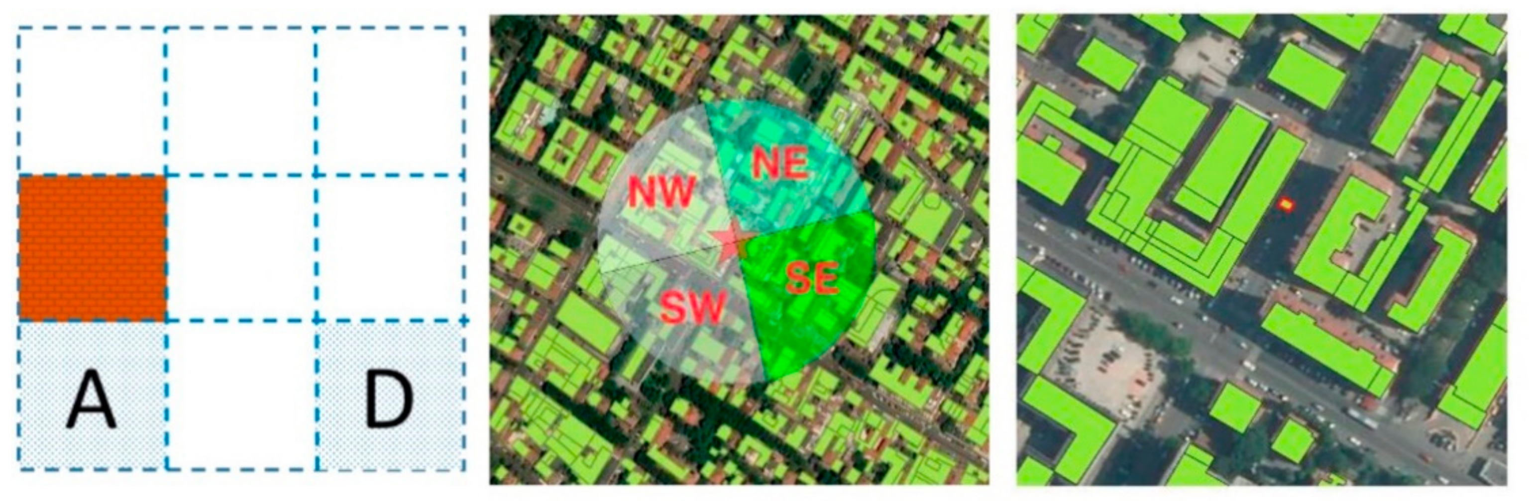
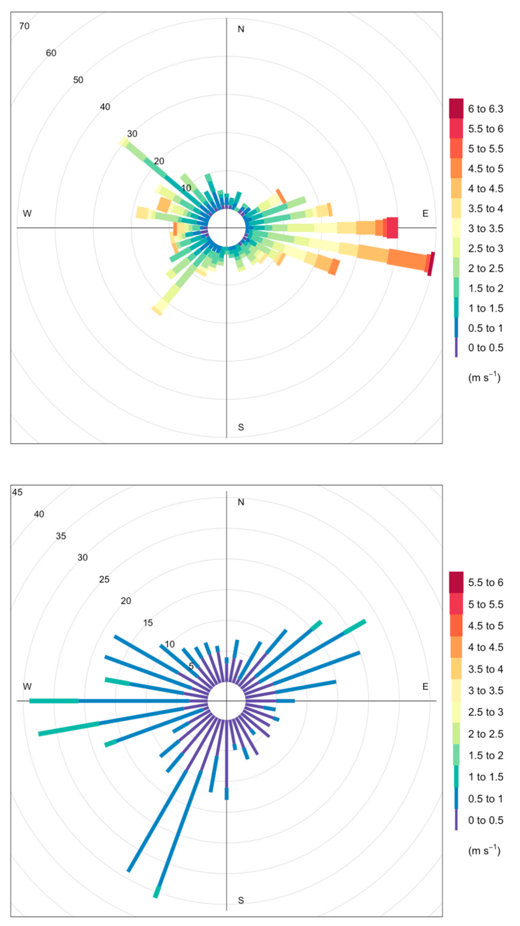
Appendix A.1. Viale Verdi Orientation and Geographical Sectors

To assess the model performances and to assess the pollutant reductions, we compared the simulated concentrations with measurements. In particular, we took into consideration features like the orientation of viale Verdi with respect to the northerly direction (about 32° northward) to define four sectors of wind direction, which are parallel to viale Verdi:
  • NE (347–77°),
  • SW (167–257°);
and perpendicular:
  • NW (257–347°),
  • SE (77–167°).
To examine the air pollutant reduction caused by the CT, we decided to study two cells of the simulation domain: A and D as indicated in Figure A1. The points were both close to the cell that represents the CT in the model grid: point A is adjacent to the CT and can be considered as representative of the air volume directly in contact with the CT, while point D is more related to the air volume within the street canyon. Point D is only four meters away from point A.
Figure A1. Left: positions of the A and D points with respect to the CT indicated here with the brown square. Centre: sectors considered according to the viale Verdi orientation. Right: position of the CT, in red, and the buildings and streets nearby.
Atmosphere 12 00839 g0a1

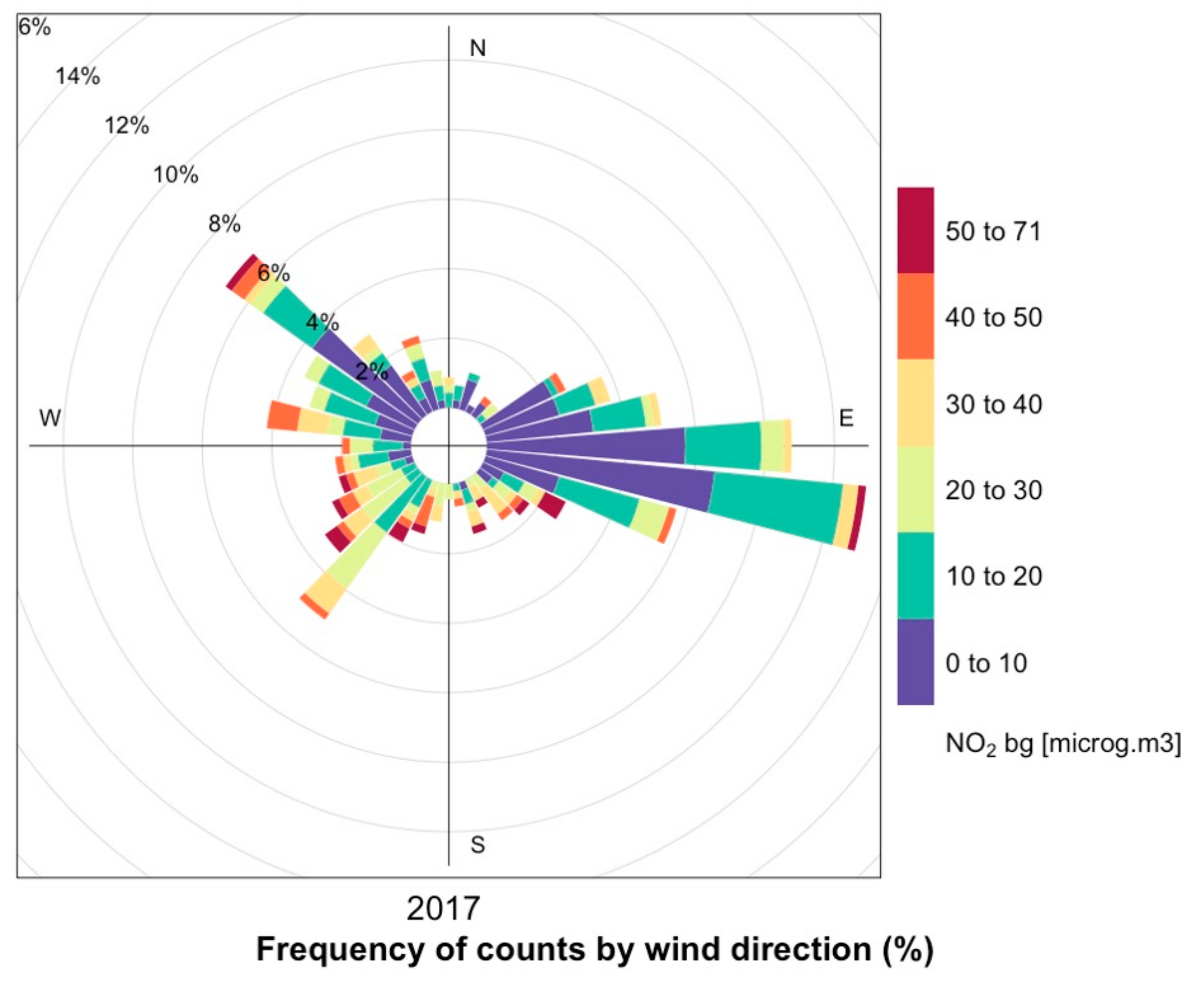
Appendix A.2. NO2 Background Concentration

We analysed the background NO2 concentration provided by the reference station in Parco Ferrari considering the wind observed at the background station Modena Urbana. The results are shown in Figure A2. According to the diagram we outline:
  • The prevailing wind directions were easterly. However, significant contributions were also from north-west and south-west directions.
  • Mean NO2 background concentrations were generally close to 20 μg/m3. These values were detected particularly with easterly winds, which were stronger (up to 6 m/s) than in the other directions where intensities were generally lower than 4 m/s (Figure A3).
Figure A2. Concentration wind rose diagrams expressing the dependence of Parco Ferrari background NO2 concentration on wind direction from Modena Urbana station (2017).
Atmosphere 12 00839 g0a2
The Modena city center is located in an eastward direction with respect to the station and, because of traffic restrictions, is usually affected by less traffic than the peripheral areas. Larger NO2 background concentrations, reaching hourly concentrations above 50 μg/m3, were measured with SW-SE winds of less than 3 m/s. Winds blowing from these directions carry pollutants from major traffic roads such as the motorway A1/E45, which is located about three km away from Parco Ferrari.

Appendix A.3. Wind Distributions

As a first step, we studied the wind distributions of the data measured at the stations of Modena Urbana (background station) and from the CNR and Consorzio ProAmbiente, in viale Verdi. The resulting wind rose diagrams are presented in Figure A3. When urban and local wind distributions are compared, many differences can be outlined relating to both wind directions and speed. The local wind directions were mainly between NE and SW, which was probably due to the microscale circulation driven by the presence of the buildings (see Figure A1). Wind speeds were generally lower than 2 m/s with the majority of the values below 1 m/s. Stronger wind speeds up to 2 m/s were measured with westerly and north-easterly winds, the latter corresponding to the north-related orientation of viale Verdi (see Figure A1).
Figure A3. Wind rose distribution for wind measured at Modena Urbana (top) and in viale Verdi (bottom).
Atmosphere 12 00839 g0a3

Appendix A.4. NOx Concentrations—Model Evaluation

We conducted the analyses in two steps:
  • Dataset exploration:
We applied the FAIRMODE IDL-based DELTA software tool version 5.4 [67,68] provided by the Forum for Air Quality Modelling in Europe (FAIRMODE) [67,73,74]. The tool was developed under the FAIRMODE framework specific evaluation protocols to support the use of air quality models when they are applied for officially reporting on national air pollution levels and for examining compliance with regulations (assessment, forecasting, planning) [73].
The FAIRMODE IDL-based DELTA software tool is based on an approach relying on paired modelled and monitored data to offer diagnostics of model performances using various statistical indicators and diagrams [73]. Given the nature and the time length of our case study, we applied the FAIRMODE IDL-based DELTA software tool for exploratory purposes [68] since the user can analyze different statistical metrics and diagrams.
Our dataset was composed of the measured data from the CNR group, and modelled data extracted in two points close to the green infrastructure, A and D, as seen in Figure A1.
We used the software to obtain: (i) timeseries plots, in order to analyze the dataset with respect to time; (ii) scatterplots, for the correlation between measured and modelled values, including their mean values; (iii) quantile plots, to compare the probability distributions by plotting their quantiles against each other; (iv) and Taylor diagrams, to quantify the degree of correspondence between the modelled and observed behaviour in terms of Pearson correlation coefficient, and the normalized standard deviation.
  • Further dataset Analysis:
We took into account hourly and daily meteorological data for a more detailed analysis by applying R-Cran library-based scripts [75], and the Taylor diagram package [70]. The meteorological measurements were provided by the station Modena Urbana (see Section 2.5), and the observed data from the CNR-Consorzio ProAmbiente measurement campaigns.
  • Exploration with the FAIRMODE IDL-based DELTA software tool
Regarding the exploration with the FAIRMODE IDL-based DELTA software tool, Figure A4, Figure A5, Figure A6 and Figure A7 show the diagrams resulting from the application of the software tool when applied in the exploratory mode to our datasets [68].
Figure A4. Timeseries diagram from FAIRMODE IDL-based DELTA software tool with hourly CNR observations (black), modelled data in A (red), and in D (green).
Atmosphere 12 00839 g0a4
The timeseries plot (Figure A4) reports on the x-axis the time in hours. The figure shows an overall good agreement in trend between observed and modelled values (e.g., see the values between the hours 3480–3570, 26 May up to 29 May 18:00). With the exception of few cases, such as the hours 3170–3180, (13 May 2017, 02:00–12:00 h), 3330 (19 May 2017, 18:00), 3560 (29 May 2017, 08:00), the modelled values are in line with the observations and in some cases they are higher than the observations (e.g., hours before 3170, 13 May 2017 02:00, and between 3390–3490, 22 May 2017 06:00 up to 26 May 2017 10:00).
From the scatterplot diagram in Figure A5 and the quantile distribution in Figure A6, measured and modelled hourly data show a dispersion that changes with the concentration values. For NOx values of less than 50 μg/m3 the two distributions are very similar and normally distributed. For higher values of NOx concentrations, the model tends to over predict, particularly when NOx concentrations are higher than 100 μg/m3. The overall R2 is quite low (0.4) in both the points A and D.
Figure A5. Scatterplot diagram from FAIRMODE IDL-based DELTA software tool with hourly modelled data in A (red), and in D (blue).
Atmosphere 12 00839 g0a5
Figure A6. Quantile plot from FAIRMODE IDL-based DELTA software tool with hourly modelled data in A (red), and in D (green).
Atmosphere 12 00839 g0a6
The Taylor diagram in Figure A7 summarizes the features of the modelled and observed distributions found in the previous plots. Here, we obtain correlation coefficients larger than 0.6 for both A and D points, the latter having R slightly larger. The ratio sigma modelled over sigma observed, e.g., normalized standard deviation is close to 1.25, indicating that the modelled values are more dispersed than the observations.
Figure A7. Taylor diagram from FAIRMODE IDL-based DELTA software tool with hourly modelled data in A (red), and in D (blue).
Atmosphere 12 00839 g0a7
  • NOx Concentration Comparisons considering Wind Directions
Figure A8 shows the comparisons between timeseries of modelled and measured CNR data with the urban wind directions in the background.
Figure A8. NOx concentrations (orange: NO2 concentration measured by the urban background station; black: observed NOx concentration; blue: NOx concentration simulated at point A, and red: NOx concentration simulated at point D) with daily prevailing wind directions from Modena Urbana according to the sectors specified in Appendix A.1. Grey vertical bands indicate rainy periods.
Atmosphere 12 00839 g0a8
Figure A9, Figure A10 and Figure A11 show the Taylor diagrams obtained for the datasets (modelled points A and D in red and blue, respectively, and the measured urban NO2 background, in green) taking the CNR data as reference measurements. Data were classified by:
  • day range within the month of May 2017 (12–16; 16–21; 21–26; and 26–31);
  • urban wind direction within four sectors (NE 347–77; NW 257–347; SE 77–167; SW 167–257);
  • local wind direction in the same four sectors as defined in Figure A1.
Figure A9. Taylor diagram with hourly modelled data in A (red), and modelled data in D (blue), and the measured background NO2 concentration (green), according to four different groups of days.
Atmosphere 12 00839 g0a9
The agreement between modelled and measured data (Figure A8) is much more evident after 25 May, where the days are generally characterized by south-easterly wind, and NOx concentrations are between 20–100 μg/m3, which are generally lower than on other days. During 26–31 May, the Taylor diagram shows the best agreement with correlation values of about 0.85 and normalized standard deviations close to one, indicating a very good agreement in the values distribution for modelled and measured data.
All the Taylor diagrams show a very good correlation with the urban background measured NO2 concentrations (green dot) which, the distribution being lower in value than the CNR observations, has a normalized standard deviation about half that of the measured one.
Figure A9 indicates that the best model performance is found during the period 12–16 May, with correlation of about 0.7 and normalized standard deviation about 1; and the period 26–31 with correlation R above 0.8 and normalized standard deviation close to 1. In the period between 16–21 and 21–26, the correlation R is between 0.5–0.6 and the normalized standard deviation is about 1.25, indicating a general over-prediction of the CNR standard deviations.
In Figure A10, NO2 concentration measured by the urban background station (green dot) is generally always well correlated with the CNR NOx measurements (correlation between 0.6 and 0.85), and it has normalized standard deviations between 0.3 (SW_167_257 sector) and 0.6 (NE 347-77 sector). With the modelled data (A in red, D in blue), the best agreement is obtained in the SW 167-257 sector with a correlation close to 0.8, and the normalized standard deviation of about 1.2. The other sectors are characterized by correlation values generally close to 0.6, and normalized standard deviation between 1.2 and 1.5.
Figure A10. Taylor diagram with hourly modelled data in A (red), and modelled data in D (blue), and the measured background NO2 concentration (green), according to the urban wind sectors defined as in Figure A1.
Atmosphere 12 00839 g0a10
Figure A11 shows background NO2 values for all the sectors (green dot) with correlations close to 0.8 and normalized standard deviation values in a limited range (0.4–0.5). Differently, the modelled data (red and blue dots) show a larger variability according to the wind sector. The best agreement is found in the SE 77–167 sector where the correlation is close to 0.8 and the normalized standard deviation is 1, followed by the SW 167–257 sector, with R close to 0.6 and normalized standard deviation slightly larger than one. Sector NE 347–77 has a correlation above 0.6, but the normalized standard deviation is larger than 1.2. The sector which shows the worst model performance is NW 257–347 where R is smaller than 0.4 and the normalized standard deviation is close to 1.8–2.
Figure A11. Taylor diagram with hourly modelled data in A (red), and modelled data in D (blue), and the measured background NO2 concentration (green), according to the local wind sectors defined as in Figure A1.
Atmosphere 12 00839 g0a11

Appendix B

Here we show a diagram (Figure A12) representing the evolution of the CT design from its first version (CT 1.0) that is the one studied in the work presented here, and the newest generations of CT (CT 2.0) available at the moment in which this paper was submitted. Different design features, such as for example the presence of a wooden cover to provide shade for the moss, have been improved and the development has been oriented at lowering the costs of operation, such as energy and water consumption. In the new CT 2.0 models, energy consumption is around 120–150 W per operating hour and water consumption is between 2 and 8 L per operating hour depending on local climate conditions. These results support the potential of CT technologies for protecting air quality in local urban contexts.
Figure A12. Timeline of the CT improvements from 2013 to present. Many design features have improved, included the use of wood in substitution of the cover plants.
Atmosphere 12 00839 g0a12

References

  1. United Nations, Department of Economic and Social Affairs, Population Division. Available online: https://population.un.org/wup/Publications/Files/WUP2014-PressRelease.pdf (accessed on 9 June 2020).
  2. Oke, T.R. Street Design and Urban Canopy Layer Climate. Energy Build. 1988, 11, 103–113. [Google Scholar] [CrossRef]
  3. Oke, T.R. Towards Better Scientific Communication in Urban Climate. Theor. Appl. Climatol. 2006, 84, 179–190. [Google Scholar] [CrossRef]
  4. AIRUSE. Air Quality Mitigation Measures in Urban Areas from Southern Europe, Report for Life Project: Airuse, Testing and Development of Air Quality Measures in South Europe, LIFE11/ENV/ES/584. Available online: https://ec.europa.eu/environment/life/project/Projects/index.cfm?fuseaction=home.showFile&rep=file&fil=LIFE11_ENV_ES_000584_LAYMAN.pdf (accessed on 11 June 2020).
  5. Bottalico, F.; Chiricia, G.; Giannetti, F.; De Marco, A.; Nocentini, S.; Paoletti, E.; Salbitano, F.; Sanesi, G.; Serenelli, C.; Travaglini, D. Air Pollution Removal by Green Infrastructures and Urban Forests in the City of Florence. Agric. Agric. Sci. Procedia 2016, 8, 243–251. [Google Scholar] [CrossRef] [Green Version]
  6. Hewitt, C.N.; Ashworth, K.; MacKenzie, A.R. Using green infrastructure to improve urban air quality (GI4AQ). Ambio 2020, 49, 62–73. [Google Scholar] [CrossRef] [PubMed] [Green Version]
  7. Jayasooriya, V.M.; Ng, A.W.M.; Muthukumaran, S.; Perera, B.J.C. Green Infrastructure Practices for Improvement of Urban Air Quality. Urban For. Urban Green. 2017, 21, 34–47. [Google Scholar] [CrossRef]
  8. Kumar, P.; Druckman, A.; Gallagher, J.; Gatersleben, B.; Allison, S.; Eisenman, T.; Hoang, U.; Hama, S.; Tiwari, A.; Sharma, A.; et al. The nexus between air pollution, green infrastructure and human health. Environ. Int. 2019, 133, 105181–105186. [Google Scholar] [CrossRef] [PubMed]
  9. Dige, G.; Eichler, L.; Vermeulen, J.; Ferreira, A.; Rademaekers, K.; Adriaenssens, V.; Kolaszewska, D. Green Infrastructure and Flood Management: Promoting Cost-Efficient Flood Risk Reduction via Green Infrastructure Solu-tions; European Environment Agency—European Union: Luxembourg, 2017; p. 14. ISBN 978-92-9213-894-3. [Google Scholar]
  10. Norton, B.A.; Coutts, A.M.; Livesley, S.J.; Harris, R.J.; Hunter, A.M.; Williams, N.S.G. Planning for cooler cities: A framework to prioritise green infrastructure to mitigate high temperatures in urban landscapes. Landsc. Urban Plan. 2016, 134, 127–138. [Google Scholar] [CrossRef]
  11. Wentworth, J. Urban Green Infrastructure. 2013. Available online: http://researchbriefings.parliament.uk/ResearchBriefing/Summary/POST-PN-448 (accessed on 20 April 2020).
  12. Chen, L.; Liu, C.; Zhang, L.; Zou, R.; Zhiqiang, Z. Variation in Tree Species Ability to Capture and Retain Airborne Fine Particulate Matter (PM2.5). Sci. Rep. 2017, 7, 3206. [Google Scholar] [CrossRef] [PubMed]
  13. Gkatsopoulos, P. A Methodology for Calculating Cooling from Vegetation Evapotranspiration for Use in Urban Space Microclimate Simulations. Procedia Environ. Sci. 2017, 38, 477–484. [Google Scholar] [CrossRef]
  14. Yu, Z.; Xu, S.; Zhang, Y.; Jørgensen, G.; Vejre, H. Strong contributions of local background climate to the cooling effect of urban green vegetation. Sci. Rep. 2018, 8, 6798. [Google Scholar] [CrossRef]
  15. Abhijith, K.V.; Kumar, P.; Gallagher, J.; McNabola, A.; Baldauf, R.; Pilla, F.; Broderick, B.; Di Sabatino, S.; Pulvirenti, B. Air pollution abatement performances of green infrastructure in open road and built-up street canyon environments—A review. Atmos. Environ. 2017, 162, 71–86. [Google Scholar] [CrossRef]
  16. Donateo, A.; Rinaldi, M.; Paglione, M.; Villani, M.G.; Russo, F.; Carbone, C.; Zanca, N.; Pappaccogli, G.; Grasso, F.M.; Busetto, M.; et al. An evaluation of the performance of a green panel in improving air quality, the case study in a street canyon in Modena, Italy. Atmos. Environ. 2021, 247, 118189. [Google Scholar] [CrossRef]
  17. Green City Solutions. Available online: https://greencitysolutions.de/en/ (accessed on 16 December 2020).
  18. Raupach, M.R.; Woods, N.; Dorr, G.; Leys, J.F.; Cleugh, H.A. The entrapment of particles by windbreaks. Atmos. Environ. 2001, 35, 3373–3383. [Google Scholar] [CrossRef]
  19. Bailey, B.N.; Stoll, R.; Pardyjak, E.R.; Mahaffee, W.F. Effect of vegetative canopy architecture on vertical transport of massless particles. Atmos. Environ. 2014, 95, 480–489. [Google Scholar] [CrossRef]
  20. Chen, H.; Zou, Q.-P. Eulerian–Lagrangian flow-vegetation interaction model using immersed boundary method and OpenFOAM. Adv. Water Resour. 2019, 126, 176–192. [Google Scholar] [CrossRef]
  21. Huai, W.; Yang, L.; Wang, W.-J.; Guo, Y.; Wang, T.; Cheng, Y.-G. Predicting the vertical low suspended sediment concentration in vegetated flow using a random displacement model. J. Hydrol. 2019, 578, 124101. [Google Scholar] [CrossRef]
  22. Liu, D.; Zheng, Y.; Chen, Q. Simulation of flow around rigid vegetation stems with a fast method of high accuracy. J. Fluids Struct. 2016, 63, 1–15. [Google Scholar] [CrossRef] [Green Version]
  23. Lu, J.; Dai, H.C. Three dimensional numerical modeling of flows and scalar transport in a vegetated channel. J. Hydro Environ. Res. 2017, 16, 27–33. [Google Scholar] [CrossRef]
  24. Martin, P.H. Exchanges between structured canopies and their physical environment: A simple analytical solution for a generic configuration. Ecol. Model. 1999, 122, 1–24. [Google Scholar] [CrossRef]
  25. Chang, T.-J.; Kao, H.-M.; Wu, Y.-T.; Huang, W.-H. Transport mechanisms of coarse, fine, and very fine particulate matter in urban street canopies with different building layouts. J. Air Waste Manag. Assoc. 2009, 59, 196–206. [Google Scholar] [CrossRef]
  26. Lonati, G.; Pepe, N.; Pirovano, G.; Balzarini, A.; Toppetti, A.; Riva, G.M. Combined Eulerian-Lagrangian Hybrid Modelling System for PM2.5 and Elemental Carbon Source Apportionment at the Urban Scale in Milan. Atmosphere 2020, 11, 1078. [Google Scholar] [CrossRef]
  27. Pepe, N.; Pirovano, G.; Balzarini, A.; Toppetti, A.; Riva, G.M.; Lonati, G. Enhanced Air Quality Modelling through AUSTAL2000 Model in Milan Urban Area. In IOP Conference Series: Earth and Environmental Science; IOP Publishing: Bristol, UK, 2019; p. 012012. [Google Scholar] [CrossRef]
  28. Wilson, J.D.; Yee, E.; Ek, N.; d’Amours, R. Lagrangian simulation of wind transport in the urban environment. Q. J. R. Meteorol. Soc. 2009, 135, 1586–1602. [Google Scholar] [CrossRef]
  29. Anfossi, D.; Tinarelli, G.; Trini Castelli, S.; Nibart, M.; Olry, C.; Commanay, J. A New Lagrangian Particle Model for the Simulation of Dense Gas Dispersion. Atmos. Environ. 2010, 44, 753–762. [Google Scholar] [CrossRef]
  30. Nibart, M.; Armand, P.; Duchenne, C.; Olry, C.; Albergel, A.; Moussafir, J.; Oldrini, O. Flow and Dispersion Modelling in a Complex Urban District Taking account of the Underground Roads Connections. In Proceedings of the 17th International Conference on Harmonisation within Atmospheric Dispersion Modelling for Regulatory Purposes, Budapest, Hungary, 9–12 May 2016. [Google Scholar]
  31. Oldrini, O.; Armand, P.; Duchenne, C.; Olry, C.; Moussafir, J.; Tinarelli, G. Description and Preliminary Validation of the PMSS Fast Response Parallel Atmospheric Flow and Dispersion Solver in Complex Built-Up Areas. Environ. Fluid Mech. 2017, 17, 997–1014. [Google Scholar] [CrossRef]
  32. Tinarelli, G.; Mortarini, L.; Castelli, S.T.; Carlino, G.; Moussafir, J.; Olry, C.; Armand, P.; Anfossi, D. Review and Validation of Microspray, a Lagrangian Particle Model of Turbulent Dispersion. Geophys. Monogr. Ser. 2012, 200, 311–327. [Google Scholar] [CrossRef]
  33. Tinarelli, G.; Gomez, F. PSPRAY General Description and User’s Guide, 2017. Version Code 3.7.3. ARIANET/ARIA Technologies. Unpublished work. 2017.
  34. Castelli, S.T.; Tinarelli, G.; Reisin, T.G. Comparison of Atmospheric Modelling Systems Simulating the Flow, Turbulence and Dispersion at the Microscale within Obstacles. Environ. Fluid Mech. 2017, 17, 879–901. [Google Scholar] [CrossRef]
  35. Bigi, A.; Veratti, G.; Fabbi, S.; Po, L.; Ghermandi, G. Forecast of the impact by local emissions at an urban micro scale by the combination of Lagrangian modelling and low cost sensing technology: The TRAFAIR project. In Proceedings of the 19th International Conference on Harmonisation within Atmospheric Dispersion Modelling for Regulatory Purposes, Harmo, Bruges, Belgium, 3–6 June 2019. [Google Scholar]
  36. Fabbi, S.; Asaro, S.; Bigi, A.; Teggi, S.; Ghermandi, G. Impact of vehicular emissions in an urban area of the Po valley by microscale simulation with the GRAL dispersion model. In IOP Conference Series: Earth and Environmental Science; IOP Publishing: Bristol, UK, 2019; Volume 296, p. 012006. [Google Scholar]
  37. Ghermandi, G.; Fabbi, S.; Bigi, A.; Veratti, G.; Despini, F.; Teggi, S.; Barbieri, C.; Torreggiani, L. Impact assessment of vehicular exhaust emissions by microscale simulation using automatic traffic flow measurements. Atmos. Pollut. Res. 2019, 10, 1473–1481. [Google Scholar] [CrossRef]
  38. Ghermandi, G.; Fabbi, S.; Veratti, G.; Bigi, A.; Teggi, S. Estimate of Secondary NO2 Levels at Two Urban Traffic Sites Using Observations and Modelling. Sustainability 2020, 12, 7897. [Google Scholar] [CrossRef]
  39. Gomez, F.; Ribstein, B.; Makké, L.; Armand, P.; Moussafir, J.; Nibart, M. Simulation of a dense gas chlorine release with a Lagrangian particle dispersion model (LPDM). Atmos. Environ. 2021, 244, 117791. [Google Scholar] [CrossRef]
  40. Oldrini, O.; Armand, P. Validation and Sensitivity Study of the PMSS Modelling System for Puff Releases in the Joint Urban 2003 Field Experiment. Bound. Layer Meteorol. 2019, 171, 513–535. [Google Scholar] [CrossRef]
  41. Oldrini, O.; Armand, P.; Duchenne, C.; Perdriel, S. Parallelization Performances of PMSS Flow and Dispersion Modeling System over a Huge Urban Area. Atmosphere 2019, 10, 404. [Google Scholar] [CrossRef] [Green Version]
  42. Tognet, F.; Turmeau, C.; Ha, T.L.; Tarnaud, E.; Rouïl, L.; Bessagnet, B.; Robine, E.; Morel, Y. Numerical modelling of microorganisms dispersion in Urban area: Application to Legionella, HARMO 2011. In Proceedings of the 14th International Conference on Harmonisation within Atmospheric Dispersion Modelling for Regulatory Purposes, Kos, Greece, 2–6 October 2011; pp. 746–750. [Google Scholar]
  43. Veratti, G.; Fabbi, S.; Bigi, A.; Lupascu, A.; Tinarelli, G.; Teggi, S.; Brusasca, G.; Butler, T.; Ghermandi, G. Towards the coupling of a chemical transport model with a micro-scale Lagrangian modelling system for evaluation of urban NOx levels in a European hotspot. Atmos. Environ. 2020, 223. [Google Scholar] [CrossRef]
  44. Bailey, B.N.; Stoll, R.; Pardyjak, E.R. A Theoretically Consistent Framework for Modelling Lagrangian Particle Deposition in Plant Canopies. Bound. Layer Meteorol. 2018, 167, 509–520. [Google Scholar] [CrossRef]
  45. Bailey, B.N.; Stoll, R. Turbulence in Sparse, Organized Vegetative Canopies: A Large-Eddy Simulation Study. Bound. Layer Meteorol. 2013, 147, 369–400. [Google Scholar] [CrossRef]
  46. Mack, A.; Duyzer, J. The Impact of City Trees on Air Quality in the Valkenburgerstraat (Amsterdam), TNO Report, TNO 2019 R10497. Available online: https://www.oudestadt.nl/wp-content/uploads/2019/06/TNO%202018%20R10613%20Rapport%20Luchtkwaliteit_6%20juni_finaal_tcm318-398657.pdf (accessed on 20 April 2020).
  47. Zhang, Z.; Chen, Q. Comparison of the Eulerian and Lagrangian Methods for Predicting Particle Transport in Enclosed Spaces. Atmos. Environ. 2007, 1, 5236–5248. [Google Scholar] [CrossRef]
  48. Béghein, C.; Jiang, Y.; Chen, Q.Y. Using Large Eddy Simulation to Study Particle Motions in a Room. Indoor Air 2005, 15, 281–290. [Google Scholar] [CrossRef] [Green Version]
  49. Lu, W.; Howarth, A.T.; Adam, N.; Rifat, S.B. Modelling and Measurement of Airflow and Aerosol Particle Distribution in a Ventilated Two-Zone Chamber. Build. Environ. 1996, 31, 417–423. [Google Scholar] [CrossRef]
  50. Zhang, Z.; Chen, Q. Numerical Analysis of Particle Behaviors in Indoor Air using Lagrangian Method. In Air Distribution in Rooms; Roomvent: Coimbra, Portugal, 2004; p. 134. ISBN 9729797323. [Google Scholar]
  51. Moreira, D.; Vilheno, M. Air Pollution and Turbulence: Modeling and Applications; CRC Press, Taylor and Francis Group: Milton Park, UK, 2009; p. 354. ISBN 978-1-4398-1144-3. [Google Scholar]
  52. Iannone, F.; Ambrosino, F.; Bracco, G.; De Rosa, M.; Funel, A.; Guarnieri, G.; Migliori, S.; Palombi, F.; Ponti, G.; Santomauro, G.; et al. CRESCO ENEA HPC clusters: A working example of a multifabric GPFS Spectrum Scale layout. In Proceedings of the 2019 International Conference on High Performance Computing Simulation (HPCS), Dublin, Ireland, 15–19 July 2019; pp. 1051–1052. [Google Scholar] [CrossRef]
  53. Buccolieri, R.; Santiago, J.L.; Rivas, E.; Sanchez, B. Review on urban tree modelling in CFD simulations: Aerodynamic, deposition and thermal effects. Urban For. Urban Green. 2018, 31, 212–220. [Google Scholar] [CrossRef]
  54. ARIANET. Available online: http://www.aria-net.it/ (accessed on 20 April 2020).
  55. Cotton, W.R.; Pielke, R.A.; Walko, R.L.; Liston, G.E.; Tremback, C.J.; Jiang, H.; McAnelly, R.L.; Harrington, J.Y.; Nicholls, M.E.; Carrio, G.G.; et al. RAMS 2001: Current Status and Future Directions. Meteorol. Atmos. Phys. 2003, 82, 5–29. [Google Scholar] [CrossRef]
  56. D’Elia, I.; Piersanti, A.; Briganti, G.; Cappelletti, A.; Ciancarella, L.; Peschi, E. Evaluation of Mitigation Measures for Air Quality in Italy in 2020 and 2030. Atmos. Pollut. Res. 2018, 9, 977–988. [Google Scholar] [CrossRef]
  57. Mircea, M.; Ciancarella, L.; Briganti, G.; Calori, G.; Cappelletti, A.; Cionni, I.; Costa, M.; Cremona, G.; D’Isidoro, M.; Finardi, S.; et al. Assessment of the AMS-MINNI System Capabilities to Simulate Air Quality Over Italy for the Calendar Year 2005. Atmos. Environ. 2014, 84, 178–188. [Google Scholar] [CrossRef]
  58. Mircea, M.; Grigoras, G.; D’Isidoro, M.; Righini, G.; Adani, M.; Briganti, G.; Ciancarella, L.; Cappelletti, A.; Calori, G.; Cionni, I.; et al. Impact of Grid Resolution on Aerosol Predictions: A Case Study over Italy. Aerosol Air Qual. Res. 2016, 16, 1253–1267. [Google Scholar] [CrossRef] [Green Version]
  59. Adani, M.; Piersanti, A.; Ciancarella, L.; D’Isidoro, M.; Villani, M.G.; Vitali, L. Preliminary Tests on the Sensitivity of the FORAIR_IT Air Quality Forecasting System to Different Meteorological Drivers. Atmosphere 2020, 11, 574. [Google Scholar] [CrossRef]
  60. FORAIT-IT. Available online: http://www.afs.enea.it/project/ha_forecast/ (accessed on 20 April 2020).
  61. Litschke, T.; Kuttler, W. On the Reduction of Urban Particle Concentration by Vegetation–A Review. Meteorol. Z. 2008, 17, 229–240. [Google Scholar] [CrossRef]
  62. GREENCITY SOLUTIONS. Deliverable Proof–Reports Resulting from the Finalisation of a Project Task, Work Package, Project Stage, Project as a Whole-EIT-BP17, Work Package 4: On Site Data Collection, Deliverable 1 (2018): Results of the Research Field Campaign 3; Green City Solutions GmbH: Bestensee, Germany, 2018. [Google Scholar]
  63. Splittgerber, V.; Saenger, P. The City Tree: A vertical plant wall. WIT Trans. Ecol. Environ. 2015, 198, 295–304. [Google Scholar] [CrossRef] [Green Version]
  64. Nanni, A.; Radice, P.; Smith, P. TREFIC (Traffic Emission Factors Improved Calculation) User’s Guide, Report ARIANET R2009.19, Unpublished work. 2009.
  65. Emisia, S.A. COPER-COmputer Programme to Calculate Emissions from Road Transport. 2018. Available online: https://www.emisia.com/utilities/copert/documentation/ (accessed on 11 June 2020).
  66. ARPAE. Arpae Emilia-Romagna. Available online: https://www.arpae.it/ (accessed on 20 April 2020).
  67. FAIRMODE. Forum for Air Quality Modelling in Europe. Available online: https://fairmode.jrc.ec.europa.eu/ (accessed on 20 April 2020).
  68. Thunis, P.; Cuvelier, C. DELTA Version 5.4, Concepts/User’s Guide/Diagrams, Joint Research Centre, Ispra (VA). April 2016. Available online: https://fairmode.jrc.ec.europa.eu/Document/fairmode/WG1/DELTA_UserGuide_V5_4.pdf (accessed on 9 June 2020).
  69. Carslaw, D.C.; Ropkins, K. Openair—An R Package for Air Quality Data Analysis. Environ. Model. Softw. 2012, 27, 52–61. [Google Scholar] [CrossRef]
  70. Lemon, J.; Bolker, B.; Oom, S.; Klein, E.; Rowlingson, B.; Wickham, H.; Tyagi, A.; Eterradossi, O.; Grothendieck, G.; Toews, M.; et al. R Cran Package ‘Plotrix’. Available online:https://cran.r-project.org/web/packages/plotrix/plotrix.pdf (accessed on 11 June 2020).
  71. Pettit, T.; Torpy, F.R.; Surawski, N.C.; Fleck, R.; Irga, P.J. Effective reduction of roadside air pollution with botanical biofiltration. J. Hazard. Mater. 2021, 414, 125566. [Google Scholar] [CrossRef]
  72. Rotach, M. Turbulence within and above an Urban Canopy. Ph.D. Thesis, Eidgenössischen Technischen Hochschule Zürich, Zürich, Switzerland, 1991. [Google Scholar] [CrossRef]
  73. Kushta, J.; Georgiou, G.K.; Proestos, Y.; Christoudias, T.; Thunis, P.; Savvides, C.; Papadopoulos, C.; Lelieveld, J. Evaluation of EU Air Quality Standards through Modeling and the FAIRMODE Benchmarking Methodology. Air Qual. Atmos. Health 2019, 12, 73. [Google Scholar] [CrossRef] [PubMed] [Green Version]
  74. Pisoni, E.; Guerreiro, C.; Lopez-Aparicio, S.; Guevara, M.; Tarrason, L.; Janssen, S.; Thunis, P.; Pfäfflin, F.; Piersanti, A.; Briganti, G.; et al. Supporting the Improvement of Air Quality Management Practices: The “FAIRMODE Pilot” Activity. J. Environ. Manag. 2019, 245, 122–130. [Google Scholar] [CrossRef]
  75. Carslaw, D. Openair: Tools for the Analysis of Air Pollution Data. 2020. Available online: https://cran.r-project.org/web/packages/openair/index.html (accessed on 11 June 2020).
Figure 1. Simulation domain and location of the CT unit within the urban area of Modena, which includes viale Verdi, indicated by a green line.
Atmosphere 12 00839 g001
Figure 2. Diagram showing the sampling points used to measure Bulk Deposition Velocities.
Atmosphere 12 00839 g002
Figure 3. Hourly vehicle flow modulation measured during the 2017 and the 2018 campaign.
Atmosphere 12 00839 g003
Figure 4. Map reporting PMSS domain, the CT position (red star symbol), the reference meteorological station Modena Urbana (yellow pentagon symbol) and the air quality station at Parco Ferrari (orange square symbol).
Atmosphere 12 00839 g004
Figure 5. Simulation results for the case of PM10 (top panels) and NOx (bottom panels) showing the percentage difference between the concentration simulated without and with the CT for the two simulation periods 2017 (a,c) and 2018 (b,d). The values in the legend indicate the upper limit of the corresponding interval.
Atmosphere 12 00839 g005
Figure 6. Maps for 2017 (left) and for 2018 (right) representing the areas where the percentage difference is larger than 0.1%.
Atmosphere 12 00839 g006
Figure 7. Vertical profiles for percentage difference reduction for PM10 (left panel) and NOx (right panel) in passive mode.
Atmosphere 12 00839 g007
Figure 8. Impact of the CT operating in filtration mode on the PM10 concentration (a) and an example of vertical dependence of such impact in the sampled points A and D (b). The map corresponds to the deposition velocity vd = 0.024 m/s. The numbers in the legend indicate the upper limit of the corresponding interval.
Atmosphere 12 00839 g008
Table 1. Summary of PMSS set-up.
Parameters20172018
Days Simulated12–31 May 20175–17 April 2018
Pollutant SimulatedPM10, NOxPM10, NOx
Horizontal Domain1 km × 1 km1 km × 1 km
Horizontal Resolution2 m2 m
Emissions:
Vehicle Input
Flow model for 2017 +
vehicle Measurements 2017
in viale Verdi
Flow model for 2017 +
vehicle Measurements 2018
in viale Verdi
Obstacle PositionViale Verdi 21Viale Verdi 21
Meteo InputRAMS [55]
4 km × 4 km, May 2017
RAMS [55]
4 km × 4 km, April 2018
Bulk Velocity Deposition (PM10) CT passive mode: 1st quartile, median, 3rd quartilevd ->0.0005 m/s,
0.0012 m/s,
0.003 m/s
vd -> 0.0005 m/s,
0.0012 m/s,
0.003 m/s
Bulk Velocity Deposition (PM10) CT active modeNot simulatedvd filtration ~ 0.024 m/s
Bulk Velocity Deposition (NOx) CT passive mode: 1st quartile, median, 3rd quartilevd -> 0.0004 m/s,
0.0011 m/s,
0.0025 m/s
vd -> 0.0004 m/s,
0.0011 m/s,
0.0025 m/s
Model VersionsPSWIFT-2.1.1, PSPRAY-3.7.3,
Intel16 compiler,
OPENMPI library
PSWIFT-2.1.1, PSPRAY-3.7.3, Intel16 compiler,
OPENMPI library
Publisher’s Note: MDPI stays neutral with regard to jurisdictional claims in published maps and institutional affiliations.

