Article

Quantifying the Impact of the COVID-19 Pandemic Restrictions on CO, CO2, and CH4 in Downtown Toronto Using Open-Path Fourier Transform Spectroscopy

1
Department of Physics, University of Toronto, Toronto, ON M5S 1A7, Canada
2
Jet Propulsion Laboratory, California Institute of Technology, Pasadena, CA 91109, USA
3
Air Quality Research Division, Environment and Climate Change Canada, Toronto, ON M3H 5T4, Canada
4
Climate Research Division, Environment and Climate Change Canada, Toronto, ON M3H 5T4, Canada
*
Author to whom correspondence should be addressed.
Submission received: 12 May 2021 / Revised: 21 June 2021 / Accepted: 29 June 2021 / Published: 30 June 2021
(This article belongs to the Special Issue Coronavirus Pandemic Shutdown Effects on Urban Air Quality)

Abstract

:
During the global COVID-19 pandemic, anthropogenic emissions of air pollutants and greenhouse gases (GHGs), especially traffic emissions in urban areas, have declined. Long-term measurements of trace gas concentrations in urban areas can be used to quantify the impact of emission reductions on GHG mole fractions. Open-path Fourier transform infrared (OP-FTIR) spectroscopy is a non-intrusive technique that can be used to simultaneously measure multiple atmospheric trace gases in the boundary layer. This study investigates the reduction of mole fractions and mole fraction enhancements above background for surface CO, CO 2 , and CH 4 in downtown Toronto, Canada (the fourth largest city in North America) during the 2020 and 2021 COVID-19 stay-at-home periods. Mean values obtained from these periods were compared with mean values from a reference period prior to the 2020 restrictions. Mean CO mole fraction enhancement declined by 51 ± 23% and 42 ± 24% during the 2020 and 2021 stay-at-home periods, respectively. The mean afternoon CO 2 mole fraction enhancement declined by 3.9 ± 2.6 ppm (36 ± 24%) and 3.5 ± 2.8 ppm (33 ± 26%) during the stay-at-home periods in 2020 and 2021. In contrast, CH 4 mole fraction enhancement did not show any significant decrease. Diurnal variation in CO during the stay-at-home period in 2020 was also significantly reduced relative to the reference period in 2020. These reductions in trace gas mole fraction enhancements coincide with the decline of local traffic during the stay-at-home periods, with an estimated reduction in CO and CO 2 enhancements of 0.74 ± 0.15 ppb and 0.18 ± 0.05 ppm per percentage decrease in traffic, respectively.

1. Introduction

The World Health Organization (WHO) declared COVID-19 a pandemic on 11 March, 2020. Since then, many countries and regions have implemented restrictions on travel and other activities to suppress the spread of the virus. As of 1 May 2021, almost 151 million cases have been confirmed around the world (https://covid19.who.int/, accessed on 29 June 2021). Emissions of air pollutants related to travel and industrial activities have declined, especially for urban regions, during the COVID-19 restrictions. These impacts are of interest to air quality and climate research, and have been investigated in many cities around the world [1]. Global data show that fossil fuel carbon dioxide (CO 2 ) and nitrogen oxides (NO x = NO + NO 2 ) emissions declined during the COVID-19 pandemic restrictions in 2020, with a maximum of 30% in mid-April 2020, due to reduced activity in the transport sector [2]. That study also noted that changes in methane (CH 4 ) emissions are mainly driven by reductions in the power sector emission, which have been smaller than those in the transport sector globally [2]. Nitrogen dioxide (NO 2 ) is an important air pollutant in urban and industrial regions. Due to the short atmospheric lifetime of NO 2 and fuel combustion as its major anthropogenic source, NO 2 reductions have been observed and quantified over urban regions around the world using satellite observations [3,4,5,6,7,8,9,10,11,12]. Reported NO 2 total column reductions vary by region and are as large as 69% compared to the period before the lockdowns or to the same period in 2019. NO 2 surface mole fractions in urban regions have been quantified using in situ data from ground stations [13,14,15,16,17,18,19,20,21,22,23,24,25,26,27,28,29,30,31,32,33,34], with reported mean reductions typically in the range from 30% to 83%. Fine particulate matter (PM 2.5 ) and surface ozone are also important air pollutants with negative health impact, but highly nonlinear atmospheric chemistry complicates determination of the impact of emission reductions due to COVID-19 lockdowns [35,36,37].
In addition to NO x , carbon monoxide (CO) is a major air pollutant in urban regions emitted by vehicular fossil fuel combustion processes. Studies have used satellite observations to investigate the impact of COVID-19 lockdowns on CO. Field et al. analyzed CO at at 500 hPa from the NASA Atmospheric Infrared Sounder (AIRS) observation over central east China [4]. They reported that CO in 2020 was 12% lower than the 2015–2019 mean, but only 2% lower than the projected CO level due to the decreasing trend in CO since 2005. Filonchyk et al. observed reduced CO at 400 hPa from AIRS after the lockdown in east China [5]. Metya et al. studied AIRS CO at 700 hPa and reported a significant 5–6% reduction in northern-central China in February-March 2020 [10]. Fan et al. investigated the COVID-19 impact on CO concentrations over populated areas in China [38]. They reported a small change (±20%) of CO column in 2020 using the TROPOspheric Monitoring Instrument (TROPOMI) observations, and found that CO surface mole fractions from in situ measurements in 2020 were not much different from those in previous years. Furthermore, using TROPOMI, Sannigrahi et al. studied 20 cities, mostly in Europe and America, and reported that CO tropospheric columns changed from −2.24% to +1.92% during the lockdown period compared to the same period in 2019 [39]. After removing the long-term historical trends, Elshorbany et al. found decreases of less than 10% in the CO total columns measured by the Measurement of Pollution in the Troposphere (MOPITT) instrument over most of the USA [40]. The decline of CO surface mole fractions in urban regions during COVID-19 lockdowns has been reported to range from not significant to 67%, using data from ground-based in situ measurements [7,9,13,15,16,17,18,19,20,22,23,26,27,28,29,30,31,34,41,42,43,44].
Toronto is the fourth largest city in North America, and over 6 million people live in the Toronto region. The Greater Toronto Area has been subject to varying restrictions since March 2020. Consistent with current terminology of the Ontario government, the periods with the strongest restrictions were in place in 2020 and 2021 are described as “stay-at-home” periods. The first stay-at-home order enacted in Ontario in 2020 was in place from 14 March to 18 May. A 50% drop in daily traffic counts was observed across the Greater Toronto Area over this period relative to pre-lockdown levels in 2020 (Figure 1). The second stay-at-home period was implemented from 14 January to 7 March 2021, resulting in a 30% drop in daily traffic counts compared to the same pre-lockdown period in 2020. Only a few studies have examined the effect of the COVID-19 restrictions on trace gases in Toronto. Adams quantified reductions of pollutants using in situ measurements from ground-based stations over Ontario [45]. This study reported an average reduction of NO 2 surface mole fraction of 2 ppb (22%) and no significant reduction of PM 2.5 mass concentration in 2020, compared to the same period of time in 2015–2020. Goldberg et al. quantified NO 2 total column reduction over 20 North American cities using TROPOMI data and reported a 30% decline in the NO 2 column over Toronto in 2020 [6]. Furthermore, using TROPOMI, Griffin et al. quantified an NO 2 column decrease of as much 60% during the lockdown in 2020 compared to previous months, with about 25% of this decrease due to the seasonalities of solar radiation and NO x emissions in Toronto region [46]. Tian et al. showed that the average CO mole fraction in six Canadian cities decreased in March 2020 (about 40% decrease in Toronto) using surface in situ data, and the average CO mole fraction in Toronto had a significant increase (about 60%) in June 2020 [47]. Interestingly in the same study, surface NO 2 in Toronto did not show a significant decrease during the lockdown in 2020 compared to the same periods in 2019 or 2018 [47].
In addition to monitoring air quality, it is important to estimating greenhouse gas (GHG) emissions of cities for attributing anthropogenic sources of GHGs and implementing strategies of mitigating global climate change. Quantification of GHG concentrations and enhancements using ground-based measurements can be used to optimize urban GHG emission estimates and detect emission changes [48,49,50]. About 35% of Toronto’s GHG emissions in 2018 were from on-road vehicles [51]. Toronto’s long term goals of GHG reduction are 65% by 2030 and net zero by 2050 [51]. To achieve this goal, public transit and personal vehicles are shifting to use low or zero-carbon energy sources [52]. Significantly reduced on-road traffic during the COVID-19 restrictions in 2020 and 2021 provides an opportunity to observe how air pollutants and GHGs may be reduced in the future as transportation switches to electric vehicles in Toronto.
OP-FTIR spectroscopy is a non-intrusive technique that can be used to simultaneously measure multiple atmospheric trace gases in the boundary layer almost continuously. Open-path measurements determine path-averaged concentrations and are less sensitive to immediate local sources compared to point measurements. Due to these characteristics, OP-FTIR has been used to monitor CO, CH 4 , CO 2 and nitrous oxide (N 2 O) from traffic emissions and other urban and rural sources [53,54,55,56,57]. The goal of this study is to quantify the changes in mole fractions and enhancements of CO, CO 2 , and CH 4 in downtown Toronto during the COVID-19 stay-at-home periods in 2020 and 2021, and to determine whether this system could detect the impact of changes in urban traffic emissions on CO and CO 2 .

2. Materials and Methods

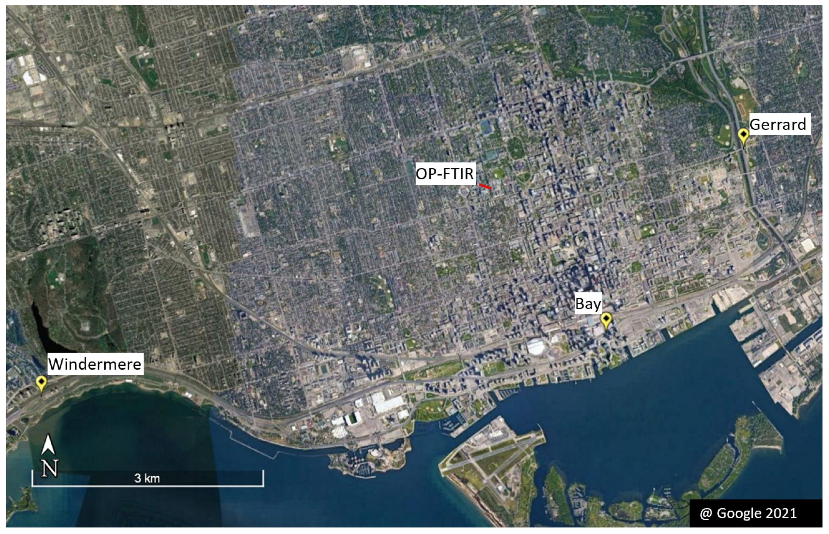
2.1. Measurements Location

The University of Toronto OP-FTIR system is located on the St. George campus in downtown Toronto, approximately 3.5 km to the north of Lake Ontario. The spectrometer, coupled with the telescope, sits in a laboratory on the twelfth floor (about 45 m above ground level (AGL)) of the McLennan Physical Laboratories building (MP). The building hosts a weather station (Vantage Pro2 Plus, Davis Instruments Corporation, Hayward, CA, USA) and a barometer (Model PTB330, Vaisala, Vantaa, Finland) on the roof (about 61 m AGL, 174 m above sea level, and located at 43.6604 N, 79.3983 W). The retro-reflector (PLX AR-30-5 corner cube array) is located on the roof of the four-storey Galbraith building (about 20 m AGL, 43.6600 N, 79.3964 W), co-located with a second weather station (Vantage Pro2 Plus, Davis Instruments Corporation). The two-way path length between the input aperture of the telescope and the retro-reflector is about 320 m. The details of this OP-FTIR instrument and the open-path optical system are described in Byrne et al. [58].

2.2. OP-FTIR Instrumentation

A Bruker IFS 125M with a CaF 2 beam-splitter (14,000–1850 cm 1 ) and an indium antimonide (InSb) detector (9600–1850 cm 1 ) records over the spectral range 1900–6000 cm 1 at 0.4 cm 1 resolution. Each measurement consists of 40 coadded scans recorded over 5 min. A 12.5-inch F/9 Ritchey-Chrétien telescope (RC Optical Systems) with gold-coated mirrors focuses the incoming infrared beam. The telescope is vertically oriented, and a 24 × 13 inch elliptical steerable mirror is located at the top of the telescope to acquire and direct the infrared beam. An infrared globar source is mounted at the top of the telescope. A shutter located in front of the globar source is alternatively raised or lowered to collect spectra with the source or from the atmosphere only. Spectra are 40 co-added scans for both shutter raised and shutter lowered measurements. Background spectra were measured when the infrared beam was directed to another retro-reflector that was previously placed at a distance about 2 meters from the steerable mirror. Measurements are made continuously day and night, with occassional gaps due to bad weather or instrumental issues.

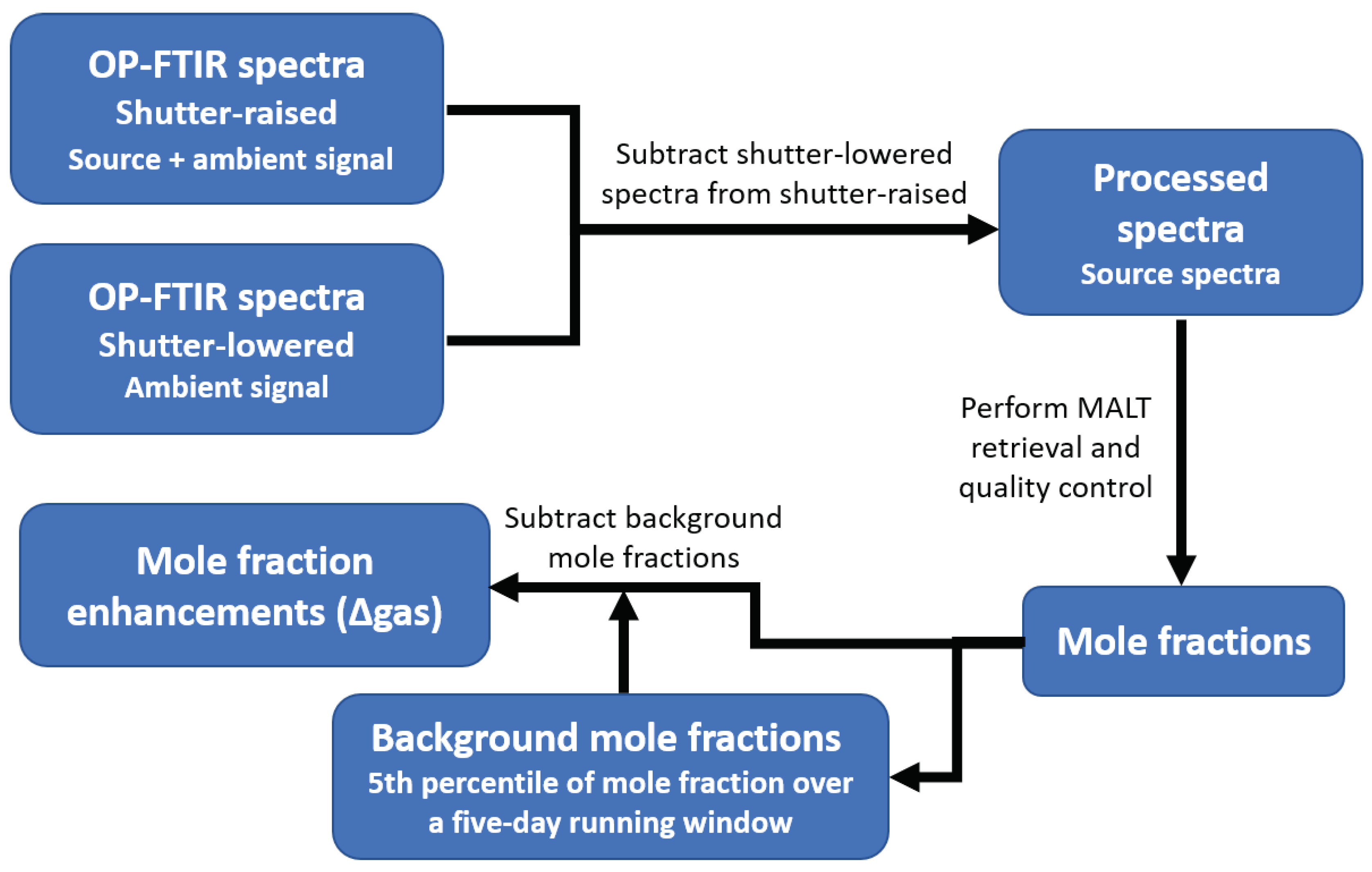
2.3. Data Processing and Gas Retrievals

The general steps of data processing in this study are shown in Figure 2. The spectra measured with the shutter raised include the globar signal as well as atmospheric emissions and scattered light from the atmosphere; the latter two signals should be subtracted from the measurement to get radiation solely from the globar source. To do this, two shutter-lowered spectra taken before and after each shutter-raised spectrum are first averaged, and then subtracted from the corresponding shutter-raised spectrum to calculate the absorption spectrum. The subtraction is similar to what is used in Byrne et al. [58], and is performed using the routine developed by Geddes et al. [59]. The transmission spectrum is then calculated by taking the ratio of this calculated absorption spectrum to a previously determined background spectrum, as described in Section 2.2.
Path-averaged mole fractions of trace gases are retrieved using the Multiple Atmospheric Layer Transmission (MALT) code version 5 [60]. In this study, the spectral line parameters are taken from the High Resolution Transmission (HITRAN) 2016 database [61]. The MALT inverse model uses non-linear least squares based on the Levenberg–Marquardt algorithm [62] to minimize root mean square (RMS) residual and obtain a best fit [63]. The input pressure is taken from the barometer measurement on the roof of MP and scaled to the height of the midpoint of the open path. The input temperature is taken from the linear interpolation of the temperature measurements on the roof of MP and beside the retro-reflector to the midpoint of the open path. There was no weather station beside the retro-reflector before November 2018, so for this period the input temperature was taken as the temperature measured on the roof of MP plus 0.45 K, considering the average temperature difference between the measurements on the roof of MP and beside the retro-reflector, and scaling to the midpoint of the open path.
In this study, CO, CO 2 and N 2 O mole fractions with respect to whole air are retrieved in the range 2141–2235 cm 1 (H 2 O is interfering gas) and CH 4 is retrieved in the range 2900–3027 cm 1 (H 2 O is interfering gas) as summarized in Table 1 [56,58]. H 2 O mole fraction is retrieved in the range 2713–2952 cm 1 [58] and used to calculate dry-air mole fractions of gases by
G A S d = G A S w 1 1 H 2 O w
where H 2 O w is the whole-air mole fraction of water retrieved by the OP-FTIR. The greatest number of the monthly 90th percentile of residual RMS (from November 2017 to March 2021) is used as the redidual RMS threshold of filtering poor measurements. The retrieved mole fractions with residual RMS > 0.0073 for CO, CO 2 and N 2 O, 0.0476 for CH 4 , and 0.0294 for H 2 O, are excluded from further analysis. Dry-air mole fractions of gases are calculated from the retrieved whole air mole fractions and H 2 O mole fractions. Dry-air mole fractions of CO, CO 2 and CH 4 are then calibrated against previous measurements using two cavity ring-down spectrometers at each end of the open-path, as described in Byrne et al. [58]. Allan deviations (ADs) are used to quantify the precision of the OP-FTIR gas retrievals [54,58], considering the atmospheric variability in mole fraction of those gases. The one hour ADs are 0.4 ppm (0.10%) for CO 2 , 1.6 ppb (0.95%) for CO, and 6.7 ppb (0.32%) for CH 4 over the entire studied period from November 2017 to March 2021. The AD results for these gases vary with the time-span of the data, because diurnal variation and short-term repeatability of mole fractions changes with time [54].

2.4. Calculating Enhancement above Background, Daily Results, and Diurnal Variation

Measured mole fractions are influenced by both local sources and long-range transport and dispersion. To investigate the impact due to changes in local sources, the mole fraction enhancement above the background is calculated for CO, CO 2 and CH 4 , since they all have significant atmospheric lifetimes [64]. In this study, the background mole fraction is defined as the 5th percentile of mole fraction of a gas over a five-day running window centered on each measurement. This running window method is used to account for the background variation from synoptic or seasonal changes. Similar running window methods have been used in previous urban studies [65,66,67]. Once the background mole fraction is calculated for each measurement, it is subtracted over the entire period of study to obtain the mole fraction enhancement above the background (e.g., Δ CO for CO) time series from 28 November 2017 to March 2021.
For the analysis in this work, three periods are defined based on the timeline of COVID-19 pandemic restrictions implemented in Toronto. Two nine-week intervals in 2018, 2019, and 2020 are defined as Period 1 and Period 2, and a seven-week interval in 2021 is defined as Period 3. The 2020 stay-at-home period from 14 March to 18 May is defined as Period 2, while Period 1 is a reference interval prior to the 2020 pandemic restrictions that has the same length as Period 2, corresponding to 13 January to 13 March. Exactly the same dates define Period 1 and Period 2 in 2018 and 2019 to enable comparisons. Finally, the 2021 stay-at-home period from 14 January to 7 March is defined as Period 3. The dates for those periods are listed in Table 2. For quantitative comparisons of CO, CO 2 and CH 4 in those periods, daily mole fractions and enhancements above background in the afternoon (from 12:00 to 16:00 local time) from the OP-FTIR measurements were extracted and averaged into daily results. The uncertainty of the difference between periods shown in this study is the 95% confidence interval of the difference in means (Table 3).
To quantify the amplitude of diurnal variations of Δ CO for these periods, the daily Δ CO peak on weekdays is calculated as
Δ CO peak = Δ CO ( h i g h ) Δ CO ( l o w )
where (all times are local time)
Δ CO ( h i g h ) = Δ CO ( average from 8 to 9 AM )
Δ CO ( l o w ) = Δ CO ( average from 3 to 6 AM )
except for 2020 Period 2, for which
Δ CO ( h i g h ) = Δ CO ( average from 7 to 8 AM )
Δ CO ( l o w ) = Δ CO ( average from 3 to 6 AM )

3. Results and Discussion

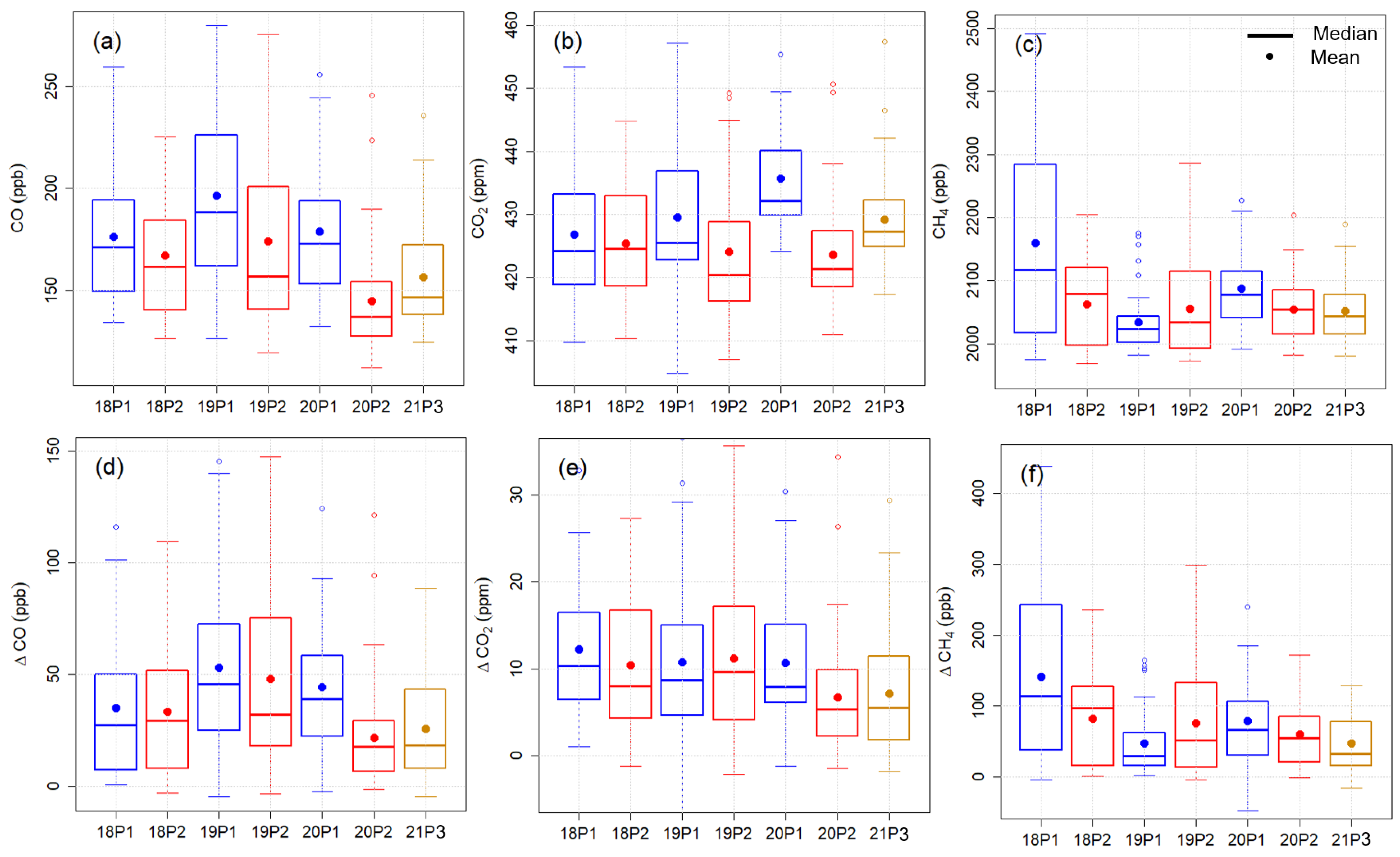
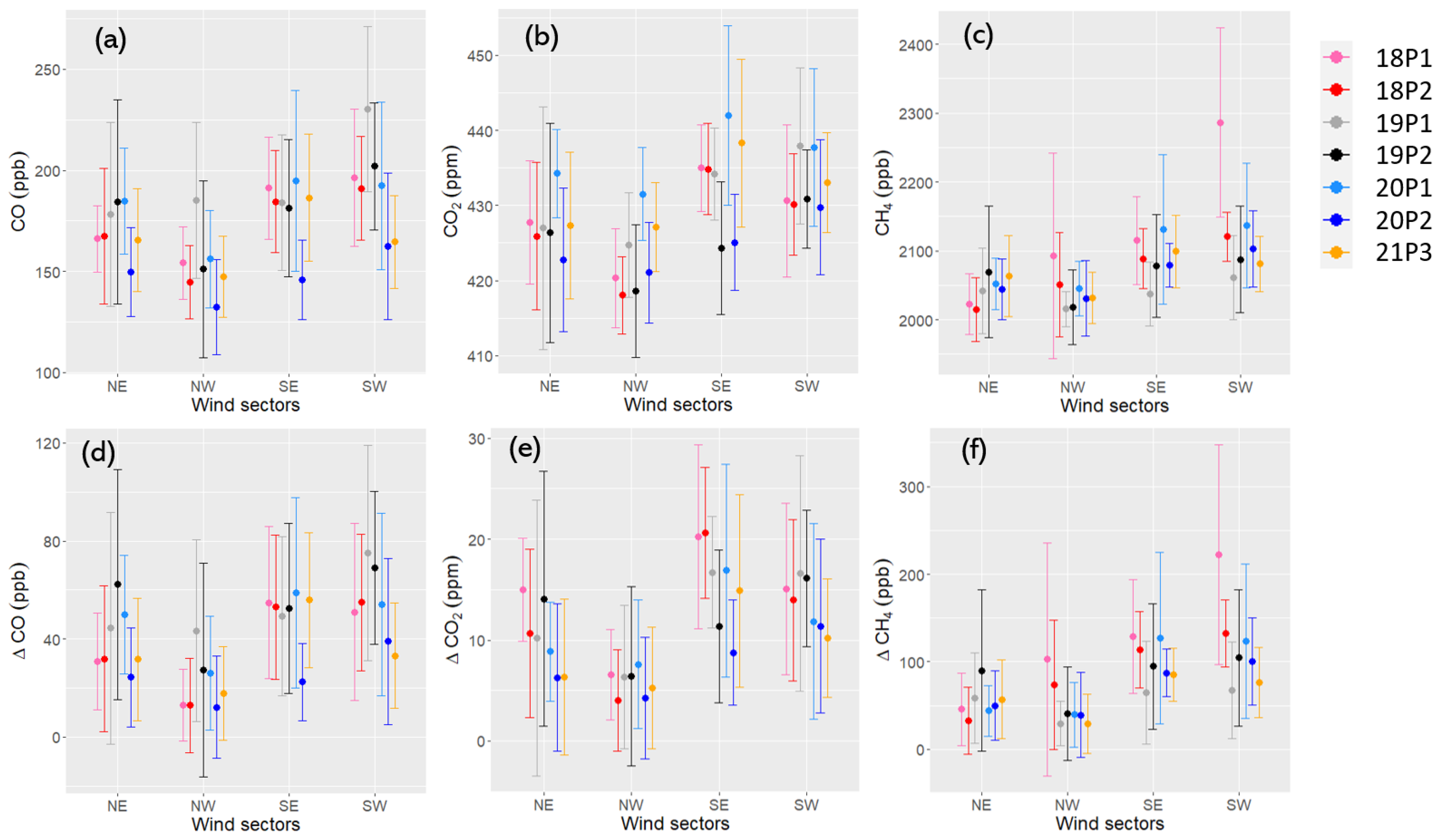
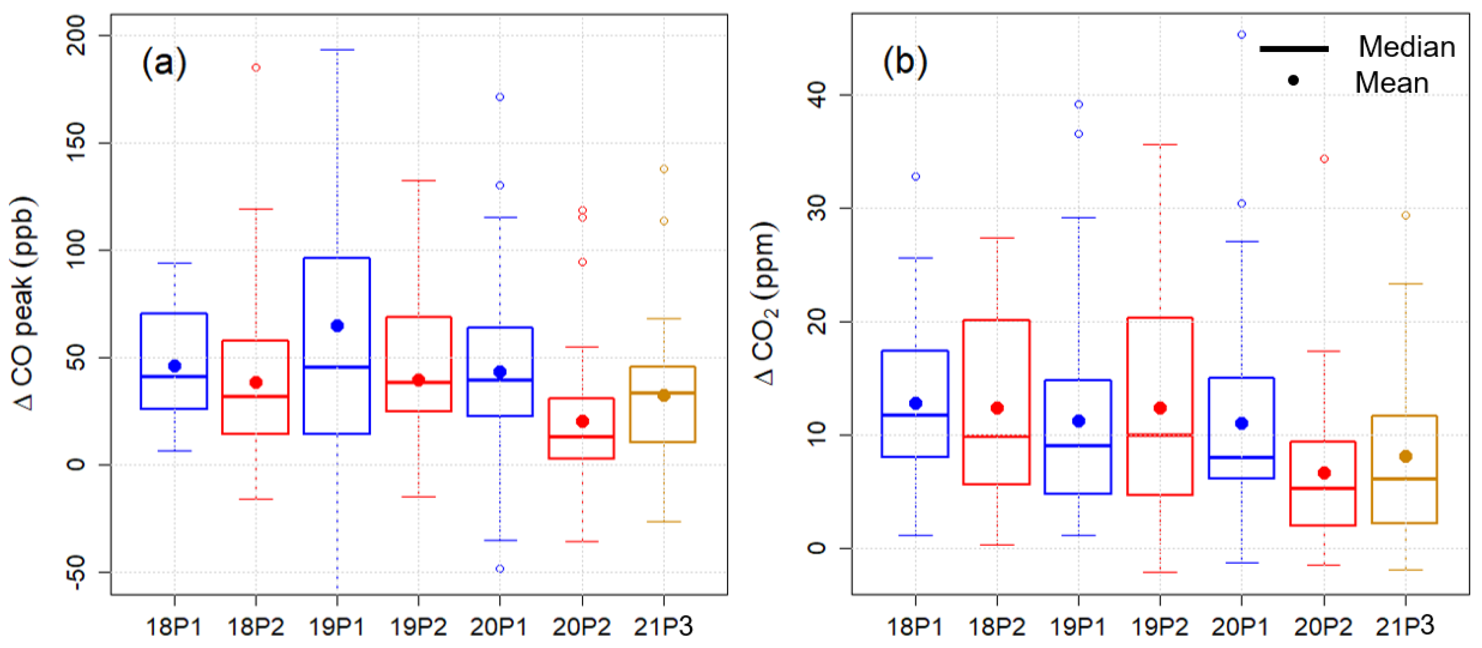
3.1. Daily Mole Fractions and Enhancements above Background

The mean daily afternoon CO mole fraction shows a decline of 19 ± 6% and 11 ± 9% for Period 2 relative to Period 1 in 2020 and 2019, respectively, (Figure 3a). The mean daily afternoon Δ CO for 2020 Period 2 declined by 51 ± 23% relative to 2020 Period 1 (Figure 3d), while the difference in Δ CO was not significant in 2019. Δ CO for 2020 Period 2 also shows declines by 55 ± 26% and 35 ± 30% relative to 2019 and 2018 Period 2, respectively. Although the mean afternoon CO during 2021 Period 3 (stay-at-home period) is greater than that during 2020 Period 2 (stay-at-home period), it still shows a significant decline of 12 ± 7% (42 ± 24% for Δ CO) relative to 2020 Period 1. This is consistent with more traffic during 2021 Period 3 than during 2020 Period 2, but is still about 30% less than 2020 Period 1 (Figure 1). The observed reductions of CO and Δ CO in this study during the two stay-at-home periods are close to previously reported urban surface CO reduction during similar periods, including a 17% reduction of mole fraction at a roadside station in Seattle, USA [30], a 25% average reduction of mole fraction enhancement from ground-based observations in California, USA [9], a 23% reduction of surface concentration in Wuhan, China [27], and a 35% reduction of surface concentration at a site located in the historical center of Athens, Greece [18].
As shown in Table 3 and Figure 3e, only in 2020 is the difference of mean Δ CO 2 between Period 1 and Period 2 significant. The mean Δ CO 2 declined by 3.9 ± 2.6 ppm (36 ± 24%) during Period 2 compared to Period 1 in 2020. The mean Δ CO 2 in the five periods before the 2020 stay-at-home period are statistically the same. Similar with Δ CO results, the mean Δ CO 2 during the two stay-at-home periods are statistically the same. Reduced traffic and other daily anthropogenic CO 2 emissions near the site during the stay-at-home period in 2020 probably contributed to this observed reduction in surface Δ CO 2 [47,68]. Changes of CO 2 during the COVID-19 pandemic restrictions were also investigated for other cities. Grivas et al. find CO 2 enhancement due to urban emission in Athens during the 2020 lockdown decreased by 58% (9 ppm) using the in situ measurements. In addition to the impact of the COVID-19 lockdown, this observed 58% decreased in Athens was also due to the seasonal cycle of residential heating emissions [18]. Liu et al. [69] reported a much greater reduction of 41 ± 1.3 ppm (63%) CO 2 mole fraction enhancement during the 2020 lockdown in Beijing compared to the period before the lockdown, using on-road mobile measurements. We observed a smaller reduction in Δ CO 2 than Liu et al. reported, likely because measurements in Liu et al. were on-road measurements on major roads and our measurements are 20–45 m above a smaller road. In contrast to these ground-level measurements, several studies have reported difficulty in detecting changes in CO 2 over urban areas using satellite observations of column-averaged dry-air mole fraction of CO 2 (XCO 2 ) [70,71]. The largest reduction in XCO 2 reported by Chevallier et al. were about 1 ppm during the February 2020 lockdown in eastern China [70]. This indicates that reductions in emission impart a relatively local signal on CO 2 , which can be detected by OP-FTIR measurement in the boundary layer but maybe more challenging to detect in XCO 2 .
The mean daily afternoon CH 4 during 2020 Period 2 and 2021 Period 3 declined by only 1.6 ± 1.2% and 1.7 ± 1.2% respectively relative to 2020 Period 1 (Table 3 and Figure 3c). Δ CH 4 showed no significant difference between the two periods in 2020 and a decline of 41 ± 29% during 2021 Period 3 compared to 2020 Period 1 (Figure 3f). The mean daily afternoon CH 4 and Δ CH 4 during the two stay-at-home periods (2020 Period 2 and 2021 Period 3) are statistically the same. The mean afternoon CH 4 and Δ CH 4 varied between examined periods and the variability in CH 4 between periods and years is likely influenced by local sources such as the steam plant immediately to the southwest of the site [58] and several buildings to the south of the site that use natural gas for physical plant infrastructure such as hot water boilers. CH 4 and Δ CH 4 showed elevation in southwest and southeast sectors (Figure 4c,f) in Period 1 in 2018.
The meteorology was investigated during the periods of interest to assess whether the observed changes in the gases might be affected by changes in meteorology. Wind speed is investigated because it is an indicator of surface turbulent mixing and greater wind speeds may associated with smaller gas mole fractions if other conditions are similar [58]. It was found that the mean daily afternoon wind speeds for the seven periods examined are not statistically different (Figure 5a). The variations in surface temperature and solar radiation may have complex effects on the planetary boundary layer height, cloud cover, and photochemical reactions of trace gases, all of which could affect surface mole fractions and trace gas enhancements. The mean afternoon temperature of 2019 Period 1 is significantly lower than those of Period 1 in 2018 and 2020 by 3.3 and 4.5 C, respectively, (Figure 5b). However, the lower temperature in 2019 Period 1 did not significantly affect Δ CO and Δ CO 2 , since the daily afternoon mean Δ CO and Δ CO 2 are not statistically different for Period 1 and Period 2 in the same year for 2018 and 2019. The mean solar radiation for Period 1 in all four years is not statistically different, nor is it for Period 2 in 2018, 2019, and 2020 (Figure 5c). Wind direction is also considered in this study, since trace gas enhancements may show weak dependence on local wind direction [58]. Figure 4a,d show that the means of CO and Δ CO in all of the four wind direction sectors consistently declined during 2020 Period 2 compared to that for 2020 Period 1. Figure 4e shows that the mean Δ CO 2 for 2020 Period 2 is consistently the smallest in all four wind direction sectors in the seven periods examined. Although Figure 5d shows that wind direction frequency in Period 2 shifted to more NE and less SW compared to Period 1 in every year from 2018 to 2020, the differences of the relative changes of CO and Δ CO in each wind direction sector between Period 1 and Period 2 in 2020 are within the 95% confidence interval of the relative decrease of CO and Δ CO for 2020 shown in Table 3. Therefore, the change in wind direction between the two periods in 2020 is not considered to significantly contribute to the observed decline in CO and Δ CO. In addition, the stay-at-home period in 2021 covered almost the same period as Period 1 in 2018–2020. Therefore, the observed declines of Δ CO and Δ CO 2 during the stay-at-home period in 2021 (2021 Period 3) relative to 2020 Period 1 also add confidence to our conclusion that reduced traffic activities during COVID-19 stay-at-home periods significantly contributed to the observed declines of CO and CO 2 in downtown Toronto.

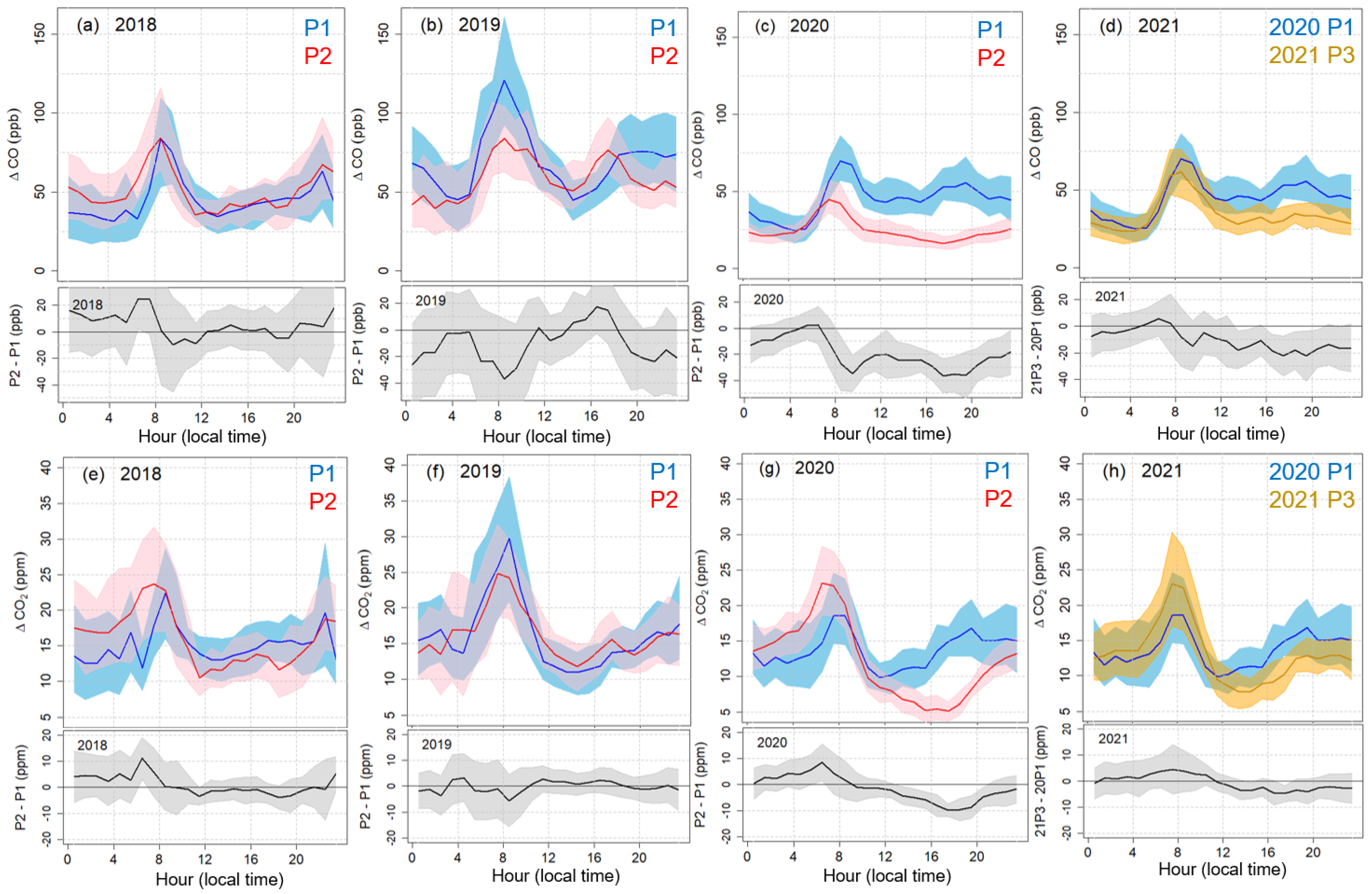
3.2. Changes in Diurnal Variations

The diurnal variation of Δ CO on weekdays for 2018 to 2021 is shown in Figure 6. Δ CO shows an early morning peak from 8 to 9 AM local time, corresponding to morning rush hour combined with low vertical mixing, and a weak enhancement after 4 PM due to the after-work rush hour in both Period 1 and Period 2 in 2018 and 2019, as well as during Period 3 (stay-at-home period) in 2021. In 2020, the diurnal cycle of Δ CO for Period 1 also showed an early morning peak from 8 to 9 AM. However, during Period 2 (the stay-at-home period) in 2020, Δ CO showed an early morning peak from 7 to 8 AM (one hour earlier) with reduced amplitude. A possible explanation for the shift of peak Δ CO during 2020 Period 2 is that the traffic count data used in this study are total counts and do not distinguish between different types of traffic. The greatest decline of traffic in downtown Toronto during the stay-at-home periods is probably in passenger commute traffic, which dominates the morning rush hour traffic counts under normal conditions. During the stay-at-home periods, traffic related to commercial or essential services may have played a bigger role, thus shifting the timing of peak Δ CO.
The statistics for the weekday daily Δ CO peak for the seven examined periods are shown in Figure 7a. Differences between any two periods are considered significant when t-test p < 0.05. The amplitude of the mean daily Δ CO peak declined by 23 ± 18 ppb (53 ± 42%) between 2020 Period 2 and 2020 Period 1, and only in 2020 is this amplitude difference significant. This reduction in the amplitude of the Δ CO early morning peak is comparable with the decline of the early morning traffic accounts on weekdays by 28–45% during the 2020 stay-at-home period (Section 3.3). Unlike 2020, the amplitude of the Δ CO early morning peak during 2021 Period 3 did not significantly decline compared to that in 2020 Period 1 (Figure 6d and Figure 7a), probably because of the smaller decline in early morning traffic (Section 3.3). 72% of CO emissions in Ontario are from transportation and mobile equipment and half of this sector is due to on-road vehicles, according to the Canada’s Air Pollutant Emission Inventory for 2018 [72]. Therefore, reduced early morning traffic during the 2020 stay-at-home period is likely to have had a significant impact on CO emissions and was coincident with the change of CO diurnal variation at our site. Tanzer-Gruener et al. observed a similar decline of CO morning peak by 50% during the lockdown in 2020 in Pittsburgh, USA using surface network data [43]. Wu et al. also reported a sharp reduction of the CO diurnal variation at all roadside and nonroadside stations in Shanghai during the COVID-19 full lockdown in 2020, with CO at roadside stations showed greater relative declines [44]. Mor et al. showed the diurnal variation of surface CO during different phases of lockdown in 2020 in Chandigarh India, and found that the period right after the lockdown started had consistently the lowest CO concentration over the entire day, including the morning rush hour [22].
The Δ CO 2 diurnal cycle in Figure 6g shows that the early morning peak is also one hour earlier during 2020 Period 2 compared to 2020 Period 1. The amplitude of peak Δ CO 2 in all periods are not significantly different. However, in 2020 Period 2 the mean Δ CO 2 in the afternoon has the smallest values of the seven examined periods and is different than that during 2020 Period 1 (Figure 6 and Figure 7b). The different diurnal variation of Δ CO 2 during 2020 Period 2 can be explained by the change in local CO 2 sources. On-road mobile emissions contribute about 50% of Δ CO 2 in Toronto during the midday in winter (Period 1) and most of the other Δ CO 2 is from natural gas combustion for residential and commercial heating [73]. Biogenic activities start to increase in the spring growing season and their overall effect on CO 2 in the afternoon is uptake. Biogenic uptake of CO 2 can significantly offset anthropogenic CO 2 emission in the afternoon at urban environments in the summer [74,75]. During the 2020 Period 2, CO 2 anthropogenic emissions declined due to the reduced on-road mobile and commercial heating sources, thus making biogenic uptake of CO 2 observable in the afternoon. In 2018 and 2019, CO 2 from traffic emission was greater than that during 2020 Period 2, counteracting the afternoon CO 2 biogenic uptake, so the latter is not visible. The mean afternoon Δ CO 2 on weekdays during the 2021 stay-at-home period lies between that of Period 1 and 2 in 2020 (Figure 7b), consistent with the comparison of traffic counts during the three periods shown in Section 3.3. The reduction of anthropogenic CO 2 emission during the COVID-19 restrictions in 2020 was also reported for the San Francisco Bay Area [75].
The diurnal variation in Δ CH 4 (not shown) was not significant during the seven periods examined. This indicates that local traffic emission is not a significant source of CH 4 .

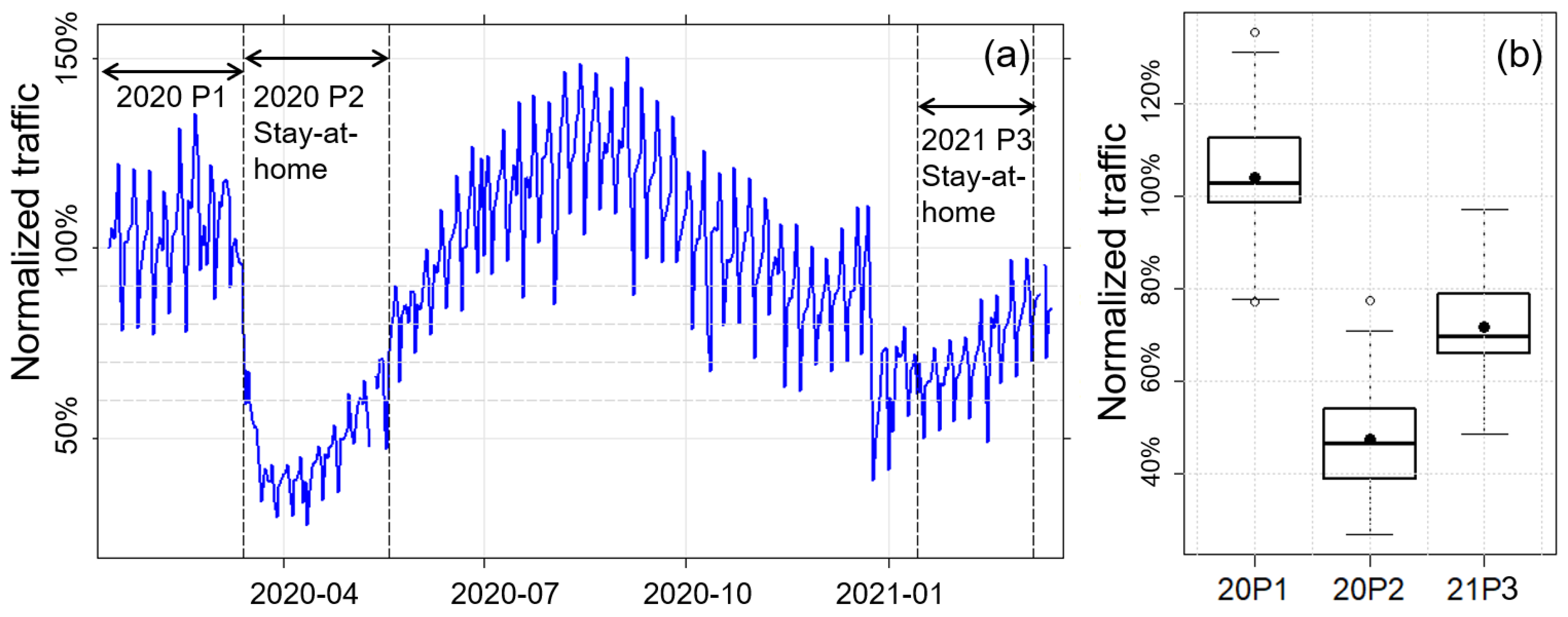
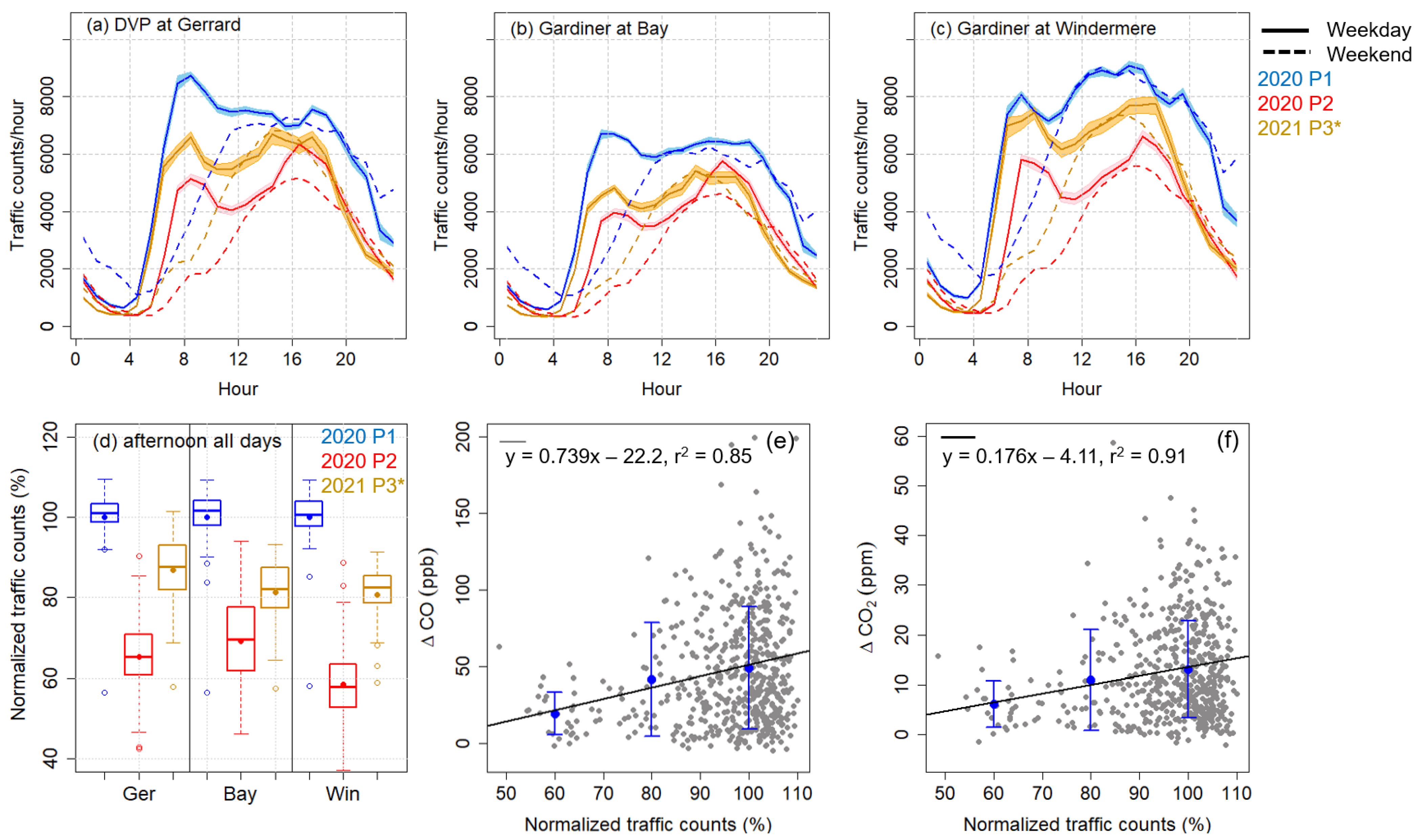
3.3. Changes in Local Traffic and Gas Enhancement from Background

The Don Valley Parkway (DVP) and the Gardiner Expressway are two major expressways in Toronto. Figure 8a–c shows the diurnal variations of traffic counts at one of the expressways with Gerrard Street, Bay Street, or Windermere Avenue. Locations of these three sites for traffic counts, as well as our OP-FTIR system, are marked in Figure 9. These data are hourly traffic counts from the City of Toronto Transportation Services. As shown in Table 4, traffic counts from 7 to 8 a.m. on weekdays at the three sites declined by 28–45% and 11–32% during the 2020 Period 2 and 2021 Period 3, respectively, compared to Period 1 in 2020. Daily afternoon (12:00 to 16:00 local time) traffic counts during 2020 and 2021 stay-at-home periods at the three sites declined by 31–41% and 13–19% respectively, compared to Period 1 in 2020 (Figure 8d and Table 4). Note that 2021 Period 3 traffic data are only available from 14 January to 18 February.
Figure 8e,f includes data over the entire study period from November 2017 to March 2021 and show a correlation between the daily afternoon Δ CO or Δ CO 2 and average normalized daily afternoon average traffic from the three traffic sites. After grouping results with normalized traffic counts in three bins, 50–70%, 70–90%, and 90–110%, linear relationships of the results of Δ CO and Δ CO 2 with traffic are observed with slopes of 0.74 ± 0.15 ppb and 0.18 ± 0.05 ppm per percentage change in traffic, respectively. These slopes are not sensitive to the way of binning data (the relative change in slopes are within 10% with different bin intervals). The uncertainty of the slopes reported here are 2 times standard deviation of the slopes calculated using the same data grouping and linear regression processes on bootstrap resampling data for 10,000 times. These slopes allow us to estimate the level of CO and CO 2 we would expect after a significant portion of the transportation sector has transitioned to electric vehicles in Toronto in the coming years. The results in this analysis indicate that this OP-FTIR system with continuous measurement is able to detect traffic emission changes of this magnitude. A limitation on the determination of the correlation between trace gas enhancements and local traffic is that the OP-FTIR site is not on an expressway and is about 2.5 to 6.2 km from the three traffic data sites used in this study. If the OP-FTIR system could be moved to a location closer to an expressway in the future, a closer correlation between trace gas enhancements and traffic counts might be obtained using the same approach employed in this study.

4. Conclusions

The OP-FTIR system used in this study detected changes in surface mole fractions and enhancements above background of CO and CO 2 in downtown Toronto during the COVID-19 stay-at-home periods in 2020 and 2021. The reductions of the mean afternoon Δ CO during the 2020 and 2021 stay-at-home periods were significant, at 23 ± 10 ppb (51 ± 23%) and 19 ± 11 ppb (42 ± 24%), respectively, compared to that for the reference period in 2020. The mean afternoon Δ CO 2 declined by 3.9 ± 2.6 ppm (36 ± 24%) and 3.5 ± 2.8 ppm (33 ± 26%) during the stay-at-home periods in 2020 and 2021 relative to the reference period in 2020, indicating the impact of reduced traffic and other local activities on CO 2 . CH 4 mole fraction enhancement above background did not show significant decline during the 2020 stay-at-home periods relative to the 2020 reference period. In addition, the mean amplitude of Δ CO diurnal variation declined by 53 ± 42% during the 2020 stay-at-home period compared to the reference period in 2020, indicating that the COVID-19 stay-at-home restrictions in Toronto in 2020 also altered the diurnal variations of CO and CO 2 . Reductions in trace gas mole fraction enhancements are coincident with the decline of local traffic during the stay-at-home periods, with Δ CO and Δ CO 2 reduced by 0.74 ± 0.15 ppb and 0.18 ± 0.05 ppm per percentage decrease in traffic, respectively. This study demonstrates a method for estimating the impact of traffic emission changes on urban surface trace gas mole fraction enhancements using continuous trace gas measurements and traffic data. The results indicate that the OP-FTIR system with continuous measurements is able to detect the decrease in traffic emissions associated with the COVID-19 restrictions, and, therefore, could be useful for assessing changes in traffic emissions after a significant portion of the transportation sector has transitioned to electric vehicles as is planned for Toronto in the coming years.

Author Contributions

Y.Y. and K.S. formulated the research goals; Y.Y., F.V. and K.S. developed the methodology; Y.Y. conducted the data analysis and wrote the initial draft, O.C. and Y.Y. collected spectral and meteorological data; F.V. provided traffic data; B.B., F.V. and K.S. significantly reviewed and edited the manuscript; R.L.M. provided OP-FTIR instruments and calibration measurements; K.S. provided financial support for this project. All authors have reviewed and agreed to the published version of the manuscript.

Funding

This research was funded by the Natural Sciences and Engineering Research Council of Canada grant number RGPIN-2019-06979, and the University of Toronto.

Institutional Review Board Statement

Not Applicable.

Informed Consent Statement

Not Applicable.

Data Availability Statement

The time series of the retrieved mole fractions of gases and meteorological parameters are available on the Scholars Portal Dataverse, https://0-doi-org.brum.beds.ac.uk/10.5683/SP2/SLNXHF [76] (accessed on 29 June 2021).

Acknowledgments

We thank the City of Toronto Transportation Services for making their data available. We thank Alex Geddes for their Python code for processing OPUS files, and Derek Mallia for the discussion of CO 2 results. We thank Environment and Climate Change Canada for the long-term loan of the OP-FTIR system under Asset Loan Agreement AQRD Tracking #244, and the Natural Sciences and Engineering Research Council of Canada. BB’s research was carried out at the Jet Propulsion Laboratory, California Institute of Technology, under a contract with the National Aeronautics and Space Administration (80NM0018D0004).

Conflicts of Interest

The authors declare no conflict of interest.

References

  1. Marinello, S.; Butturi, M.A.; Gamberini, R. How changes in human activities during the lockdown impacted air quality parameters: A review. Environ. Prog. Sustain. Energy 2021, e13672. [Google Scholar] [CrossRef]
  2. Forster, P.; Forster, H.; Evans, M.; Gidden, M.; Jones, C.; Keller, C.; Lamboll, R.; Quéré, C.; Rogelj, J.; Rosen, D.; et al. Current and future global climate impacts resulting from COVID-19. Nat. Clim. Chang. 2020, 10, 913–919. [Google Scholar] [CrossRef]
  3. Bauwens, M.; Compernolle, S.; Stavrakou, T.; Müller, J.F.; van Gent, J.; Eskes, H.; Levelt, P.F.; van der A, R.; Veefkind, J.P.; Vlietinck, J.; et al. Impact of Coronavirus Outbreak on NO2 Pollution Assessed Using TROPOMI and OMI Observations. Geophys. Res. Lett. 2020, 47, e2020GL087978. [Google Scholar] [CrossRef]
  4. Field, R.D.; Hickman, J.E.; Geogdzhayev, I.V.; Tsigaridis, K.; Bauer, S.E. Changes in satellite retrievals of atmospheric composition over eastern China during the 2020 COVID-19 lockdowns. Atmos. Chem. Phys. Discuss. 2020, 2020. [Google Scholar] [CrossRef]
  5. Filonchyk, M.; Hurynovich, V.; Yan, H.; Gusev, A.; Shpilevskaya, N. Impact assessment of COVID-19 on variations of SO2, NO2, CO and AOD over east China. Aerosol Air Qual. Res. 2020, 20, 1530–1540. [Google Scholar] [CrossRef]
  6. Goldberg, D.L.; Anenberg, S.C.; Griffin, D.; McLinden, C.A.; Lu, Z.; Streets, D.G. Disentangling the Impact of the COVID-19 Lockdowns on Urban NO2 From Natural Variability. Geophys. Res. Lett. 2020, 47, e2020GL089269. [Google Scholar] [CrossRef]
  7. Kanniah, K.D.; Kamarul Zaman, N.A.F.; Kaskaoutis, D.G.; Latif, M.T. COVID-19’s impact on the atmospheric environment in the Southeast Asia region. Sci. Total Environ. 2020, 736, 139658. [Google Scholar] [CrossRef] [PubMed]
  8. Koukouli, M.E.; Skoulidou, I.; Karavias, A.; Parcharidis, I.; Balis, D.; Manders, A.; Segers, A.; Eskes, H.; van Geffen, J. Sudden changes in nitrogen dioxide emissions over Greece due to lockdown after the outbreak of COVID-19. Atmos. Chem. Phys. 2021, 21, 1759–1774. [Google Scholar] [CrossRef]
  9. Liu, Q.; Harris, J.T.; Chiu, L.S.; Sun, D.; Houser, P.R.; Yu, M.; Duffy, D.Q.; Little, M.M.; Yang, C. Spatiotemporal impacts of COVID-19 on air pollution in California, USA. Sci. Total Environ. 2021, 750, 141592. [Google Scholar] [CrossRef]
  10. Metya, A.; Dagupta, P.; Halder, S.; Chakraborty, S.; Tiwari, Y. COVID-19 lockdowns improve air quality in the South-East Asian regions, as seen by the Remote Sens. satellites. Aerosol Air Qual. Res. 2020, 20, 1772–1782. [Google Scholar] [CrossRef]
  11. Soni, M.; Verma, S.; Jethava, H.; Payra, S.; Lamsal, L.; Gupta, P.; Singh, J. Impact of COVID-19 on the Air Quality over China and India Using Long-term (2009-2020) Multi-satellite Data. Aerosol Air Qual. Res. 2021, 21, 200295. [Google Scholar] [CrossRef]
  12. Wang, Q.; Su, M. A preliminary assessment of the impact of COVID-19 on environment—A case study of China. Sci. Total Environ. 2020, 728, 138915. [Google Scholar] [CrossRef] [PubMed]
  13. Anil, I.; Alagha, O. The impact of COVID-19 lockdown on the air quality of Eastern Province, Saudi Arabia. Air Qual. Atmos. Health 2020. [Google Scholar] [CrossRef]
  14. Baldasano, J.M. COVID-19 lockdown effects on air quality by NO2 in the cities of Barcelona and Madrid (Spain). Sci. Total Environ. 2020, 741, 140353. [Google Scholar] [CrossRef]
  15. Bedi, J.S.; Dhaka, P.; Vijay, D.; Aulakh, R.S.; Gill, J.P.S. Assessment of Air Quality Changes in the Four Metropolitan Cities of India during COVID-19 Pandemic Lockdown. Aerosol Air Qual. Res. 2020, 20, 2062–2070. [Google Scholar] [CrossRef]
  16. Broomandi, P.; Karaca, F.; Nikfal, A.; Jahanbakhshi, A.; Tamjidi, M.; Kim, J.R. Impact of COVID-19 Event on the Air Quality in Iran. Aerosol Air Qual. Res. 2020, 20, 1793–1804. [Google Scholar] [CrossRef]
  17. Dantas, G.; Siciliano, B.; França, B.; da Silva, C.; Arbilla, G. The impact of COVID-19 partial lockdown on the air quality of the city of Rio de Janeiro, Brazil. Sci. Total Environ. 2020, 729. [Google Scholar] [CrossRef]
  18. Grivas, G.; Athanasopoulou, E.; Kakouri, A.; Bailey, J.; Liakakou, E.; Stavroulas, I.; Kalkavouras, P.; Bougiatioti, A.; Kaskaoutis, D.G.; Ramonet, M.; et al. Integrating in situ Measurements and City Scale Modelling to Assess the COVID–19 Lockdown Effects on Emissions and Air Quality in Athens, Greece. Atmosphere 2020, 11, 1174. [Google Scholar] [CrossRef]
  19. Kerimray, A.; Baimatova, N.; Ibragimova, O.P.; Bukenov, B.; Kenessov, B.; Plotitsyn, P.; Karaca, F. Assessing air quality changes in large cities during COVID-19 lockdowns: The impacts of traffic-free urban conditions in Almaty, Kazakhstan. Sci. Total Environ. 2020, 730, 139179. [Google Scholar] [CrossRef] [PubMed]
  20. Li, L.; Li, Q.; Huang, L.; Wang, Q.; Zhu, A.; Xu, J.; Liu, Z.; Li, H.; Shi, L.; Li, R.; et al. Air quality changes during the COVID-19 lockdown over the Yangtze River Delta Region: An insight into the impact of human activity pattern changes on air pollution variation. Sci. Total Environ. 2020, 732. [Google Scholar] [CrossRef]
  21. Lee, J.D.; Drysdale, W.S.; Finch, D.P.; Wilde, S.E.; Palmer, P.I. UK surface NO2 levels dropped by 42% during the COVID-19 lockdown: Impact on surface O3. Atmos. Chem. Phys. 2020, 20, 15743–15759. [Google Scholar] [CrossRef]
  22. Mor, S.; Kumar, S.; Singh, T.; Dogra, S.; Pandey, V.; Ravindra, K. Impact of COVID-19 lockdown on air quality in Chandigarh, India: Understanding the emission sources during controlled anthropogenic activities. Chemosphere 2021, 263. [Google Scholar] [CrossRef] [PubMed]
  23. Nakada, L.Y.K.; Urban, R.C. COVID-19 pandemic: Impacts on the air quality during the partial lockdown in São Paulo state, Brazil. Sci. Total Environ. 2020, 730, 139087. [Google Scholar] [CrossRef] [PubMed]
  24. Patel, H.; Talbot, N.; Salmond, J.; Dirks, K.; Xie, S.; Davy, P. Implications for air quality management of changes in air quality during lockdown in Auckland (New Zealand) in response to the 2020 SARS-CoV-2 epidemic. Sci. Total Environ. 2020, 746, 141129. [Google Scholar] [CrossRef]
  25. Ropkins, K.; Tate, J. Early observations on the impact of the COVID-19 lockdown on air quality trends across the UK. Sci. Total Environ. 2021, 754. [Google Scholar] [CrossRef]
  26. Shakoor, A.; Chen, X.; Farooq, T.; Shahzad, U.; Ashraf, F.; Rehman, A.; Sahar, N.; Yan, W. Fluctuations in environmental pollutants and air quality during the lockdown in the USA and China: Two sides of COVID-19 pandemic. Air Qual. Atmos. Health 2020. [Google Scholar] [CrossRef] [PubMed]
  27. Shi, X.; Brasseur, G.P. The Response in Air Quality to the Reduction of Chinese Economic Activities During the COVID-19 Outbreak. Geophys. Res. Lett. 2020, 47, e2020GL088070. [Google Scholar] [CrossRef]
  28. Singh, V.; Singh, S.; Biswal, A.; Kesarkar, A.; Mor, S.; Ravindra, K. Diurnal and temporal changes in air pollution during COVID-19 strict lockdown over different regions of India. Environ. Pollut. 2020, 266. [Google Scholar] [CrossRef]
  29. Wyche, K.; Nichols, M.; Parfitt, H.; Beckett, P.; Gregg, D.; Smallbone, K.; Monks, P. Changes in ambient air quality and atmospheric composition and reactivity in the South East of the UK as a result of the COVID-19 lockdown. Sci. Total Environ. 2021, 755, 142526. [Google Scholar] [CrossRef]
  30. Xiang, J.; Austin, E.; Gould, T.; Larson, T.; Shirai, J.; Liu, Y.; Marshall, J.; Seto, E. Impacts of the COVID-19 responses on traffic-related air pollution in a Northwestern US city. Sci. Total Environ. 2020, 747, 141325. [Google Scholar] [CrossRef]
  31. Yuan, Q.; Qi, B.; Hu, D.; Wang, J.; Zhang, J.; Yang, H.; Zhang, S.; Liu, L.; Xu, L.; Li, W. Spatiotemporal variations and reduction of air pollutants during the COVID-19 pandemic in a megacity of Yangtze River Delta in China. Sci. Total Environ. 2021, 751, 141820. [Google Scholar] [CrossRef] [PubMed]
  32. Zalakeviciute, R.; Vasquez, R.; Bayas, D.; Buenano, A.; Mejia, D.; Zegarra, R.; Diaz, V.; Lamb, B. Drastic Improvements in Air Quality in Ecuador during the COVID-19 Outbreak. Aerosol Air Qual. Res. 2020, 20, 1783–1792. [Google Scholar] [CrossRef]
  33. Zangari, S.; Hill, D.T.; Charette, A.T.; Mirowsky, J.E. Air quality changes in New York City during the COVID-19 pandemic. Sci. Total Environ. 2020, 742, 140496. [Google Scholar] [CrossRef]
  34. Zhao, Y.; Zhang, K.; Xu, X.; Shen, H.; Zhu, X.; Zhang, Y.; Hu, Y.; Shen, G. Substantial changes in nitrogen dioxide and ozone after excluding meteorological impacts during the COVID-19 outbreak in Mainland China. Environ. Sci. Tech. Lett. 2020, 7, 402–408. [Google Scholar] [CrossRef]
  35. Kroll, J.; Heald, C.; Cappa, C.; Farmer, D.; Fry, J.; Murphy, J.; Steiner, A. The complex chemical effects of COVID-19 shutdowns on air quality. Nat. Chem. 2020, 12, 777–779. [Google Scholar] [CrossRef] [PubMed]
  36. Le, T.; Wang, Y.; Liu, L.; Yang, J.; Yung, Y.; Li, G.; Seinfeld, J. Unexpected air pollution with marked emission reductions during the COVID-19 outbreak in China. Science 2020, 369, 702–706. [Google Scholar] [CrossRef]
  37. Steinbrecht, W.; Kubistin, D.; Plass-Dülmer, C.; Davies, J.; Tarasick, D.W.; Gathen, P.V.D.; Deckelmann, H.; Jepsen, N.; Kivi, R.; Lyall, N.; et al. COVID-19 Crisis Reduces Free Tropospheric Ozone Across the Northern Hemisphere. Geophys. Res. Lett. 2021, 48, e2020GL091987. [Google Scholar] [CrossRef] [PubMed]
  38. Fan, C.; Li, Y.; Guang, J.; Li, Z.; Elnashar, A.; Allam, M.; de Leeuw, G. The impact of the control measures during the COVID-19 outbreak on air pollution in China. Remote Sens. 2020, 12, 1613. [Google Scholar] [CrossRef]
  39. Sannigrahi, S.; Kumar, P.; Molter, A.; Zhang, Q.; Basu, B.; Basu, A.; Pilla, F. Examining the status of improved air quality in world cities due to COVID-19 led temporary reduction in anthropogenic emissions. Environ. Res. 2021, 196. [Google Scholar] [CrossRef] [PubMed]
  40. Elshorbany, Y.F.; Kapper, H.C.; Ziemke, J.R.; Parr, S.A. The Status of Air Quality in the United States During the COVID-19 Pandemic: A Remote Sensing Perspective. Remote Sens. 2021, 13, 369. [Google Scholar] [CrossRef]
  41. Lian, X.; Huang, J.; Huang, R.; Liu, C.; Wang, L.; Zhang, T. Impact of city lockdown on the air quality of COVID-19-hit of Wuhan city. Sci. Total Environ. 2020, 742, 140556. [Google Scholar] [CrossRef]
  42. Marinello, S.; Lolli, F.; Gamberini, R. The Impact of the COVID-19 emergency on local vehicular traffic and its consequences for the environment: The case of the city of Reggio Emilia (Italy). Sustainability 2021, 13, 118. [Google Scholar] [CrossRef]
  43. Tanzer-Gruener, R.; Li, J.; Eilenberg, S.R.; Robinson, A.L.; Presto, A.A. Impacts of modifiable factors on ambient air pollution: A case study of COVID-19 shutdowns. Environ. Sci. Tech. Lett. 2020, 7, 554–559. [Google Scholar] [CrossRef]
  44. Wu, C.L.; Wang, H.W.; Cai, W.J.; He, H.D.; Ni, A.N.; Peng, Z.R. Impact of the COVID-19 lockdown on roadside traffic-related air pollution in Shanghai, China. Build. Environ. 2021, 194. [Google Scholar] [CrossRef] [PubMed]
  45. Adams, M. Air pollution in Ontario, Canada during the COVID-19 State of Emergency. Sci. Total Environ. 2020, 742. [Google Scholar] [CrossRef] [PubMed]
  46. Griffin, D.; McLinden, C.; Racine, J.; Moran, M.; Fioletov, V.; Pavlovic, R.; Mashayekhi, R.; Zhao, X.; Eskes, H. Assessing the impact of corona-virus-19 on nitrogen dioxide levels over southern Ontario, Canada. Remote Sens. 2020, 12, 4112. [Google Scholar] [CrossRef]
  47. Tian, X.; An, C.; Chen, Z.; Tian, Z. Assessing the impact of COVID-19 pandemic on urban transportation and air quality in Canada. Sci. Total Environ. 2021, 765. [Google Scholar] [CrossRef] [PubMed]
  48. Mitchell, L.; Crosman, E.; Jacques, A.; Fasoli, B.; Leclair-Marzolf, L.; Horel, J.; Bowling, D.; Ehleringer, J.; Lin, J. Monitoring of greenhouse gases and pollutants across an urban area using a light-rail public transit platform. Atmos. Environ. 2018, 187, 9–23. [Google Scholar] [CrossRef]
  49. Wunch, D.; Wennberg, P.O.; Toon, G.C.; Keppel-Aleks, G.; Yavin, Y.G. Emissions of greenhouse gases from a North American megacity. Geophys. Res. Lett. 2009, 36. [Google Scholar] [CrossRef] [Green Version]
  50. Ware, J.; Kort, E.A.; Duren, R.; Mueller, K.L.; Verhulst, K.; Yadav, V. Detecting Urban Emissions Changes and Events with a Near-Real-Time-Capable Inversion System. J. Geophys. Res. Atmos. 2019, 124, 5117–5130. [Google Scholar] [CrossRef]
  51. City of Toronto. 2018 Greenhouse Gas Emissions Inventory. 2018. Available online: https://www.toronto.ca/wp-content/uploads/2020/12/9525-2018-GHG-Inventory-Report-Final-Published.pdf (accessed on 16 April 2021).
  52. City of Toronto. TransformTO: 2019 Implementation Update. 2020. Available online: https://www.toronto.ca/wp-content/uploads/2020/11/96aa-TTO-2019-Update-June2020-FINAL-AODA.pdf (accessed on 27 April 2021).
  53. Deutscher, N.M.; Naylor, T.A.; Caldow, C.G.R.; McDougall, H.L.; Carter, A.G.; Griffith, D.W.T. Performance of an open-path near-infrared measurement system for measurements of CO2 and CH4 during extended field trials. Atmos. Meas. Tech. 2021, 14, 3119–3130. [Google Scholar] [CrossRef]
  54. Griffith, D.W.T.; Pöhler, D.; Schmitt, S.; Hammer, S.; Vardag, S.N.; Platt, U. Long open-path measurements of greenhouse gases in air using near-infrared Fourier transform spectroscopy. Atmos. Meas. Tech. 2018, 11, 1549–1563. [Google Scholar] [CrossRef] [Green Version]
  55. Grutter, M.; Flores, E.; Basaldud, R.; Ruiz-Suarez, L.G. Open-path FTIR spectroscopic studies of the trace gases over Mexico City. Atmos. Ocean. Opt. 2003, 16, 232–236. [Google Scholar]
  56. Wiacek, A.; Li, L.; Tobin, K.; Mitchell, M. Characterization of trace gas emissions at an intermediate port. Atmos. Chem. Phys. 2018, 18, 13787–13812. [Google Scholar] [CrossRef] [Green Version]
  57. You, Y.; Staebler, R.M.; Moussa, S.G.; Su, Y.; Munoz, T.; Stroud, C.; Zhang, J.; Moran, M.D. Long-path measurements of pollutants and micrometeorology over Highway 401 in Toronto. Atmos. Chem. Phys. 2017, 17, 14119–14143. [Google Scholar] [CrossRef] [Green Version]
  58. Byrne, B.; Strong, K.; Colebatch, O.; You, Y.; Wunch, D.; Ars, S.; Jones, D.B.A.; Fogal, P.; Mittermeier, R.L.; Worthy, D.; et al. Monitoring urban greenhouse gases using open-path Fourier transform spectroscopy. Atmos. Ocean 2020, 58, 25–45. [Google Scholar] [CrossRef]
  59. Geddes, A.; Robinson, J.; Smale, D. Python-based dynamic scheduling assistant for atmospheric measurements by Bruker instruments using OPUS. Appl. Opt. 2018, 57, 689–691. [Google Scholar] [CrossRef] [PubMed]
  60. Griffith, D.W.T. Synthetic calibration and quantitative analysis of gas-phase FT-IR spectra. Appl. Spectrosc. 1996, 50, 59–70. [Google Scholar] [CrossRef]
  61. Gordon, I.; Rothman, L.; Hill, C.; Kochanov, R.; Tan, Y.; Bernath, P.; Birk, M.; Boudon, V.; Campargue, A.; Chance, K.; et al. The HITRAN2016 molecular spectroscopic database. J. Quant. Spectrosc. Radiat. Transf. 2017, 203, 3–69. [Google Scholar] [CrossRef]
  62. Press, W.H.; Teukolsky, S.A.; Vetterling, W.T.; Flannery, B.P. Numerical Recipes in C++; Cambridge University Press: New York, NY, USA, 1992. [Google Scholar]
  63. Griffith, D.W.T.; Deutscher, N.M.; Caldow, C.; Kettlewell, G.; Riggenbach, M.; Hammer, S. A Fourier transform infrared trace gas and isotope analyser for atmospheric applications. Atmos. Meas. Tech. 2012, 5, 2481–2498. [Google Scholar] [CrossRef] [Green Version]
  64. Jacob, D.J. Introduction to Atmospheric Chemistry; Princeton University Press: Princeton, NJ, USA, 1999; pp. 199–211. [Google Scholar]
  65. Ammoura, L.; Xueref-Remy, I.; Vogel, F.; Gros, V.; Baudic, A.; Bonsang, B.; Delmotte, M.; Té, Y.; Chevallier, F. Exploiting stagnant conditions to derive robust emission ratio estimates for CO2, CO and volatile organic compounds in Paris. Atmos. Chem. Phys. 2016, 16, 15653–15664. [Google Scholar] [CrossRef] [Green Version]
  66. Bares, R.; Lin, J.; Hoch, S.; Baasandorj, M.; Mendoza, D.; Fasoli, B.; Mitchell, L.; Catharine, D.; Stephens, B. The wintertime covariation of CO2 and criteria pollutants in an urban valley of the Western United States. J. Geophys. Res. Atmos. 2018, 123, 2684–2703. [Google Scholar] [CrossRef]
  67. Super, I.; Denier van der Gon, H.A.C.; van der Molen, M.K.; Sterk, H.A.M.; Hensen, A.; Peters, W. A multi-model approach to monitor emissions of CO2 and CO from an urban–industrial complex. Atmos. Chem. Phys. 2017, 17, 13297–13316. [Google Scholar] [CrossRef] [Green Version]
  68. Le Quéré, C.; Jackson, R.; Jones, M.; Smith, A.; Abernethy, S.; Andrew, R.; De-Gol, A.; Willis, D.; Shan, Y.; Canadell, J.; et al. Temporary reduction in daily global CO2 emissions during the COVID-19 forced confinement. Nat. Clim. Chang. 2020, 10, 647–653. [Google Scholar] [CrossRef]
  69. Liu, D.; Sun, W.; Zeng, N.; Han, P.; Yao, B.; Liu, Z.; Wang, P.; Zheng, K.; Mei, H.; Cai, Q. Observed decreases in on-road CO2 concentrations in Beijing during COVID-19 restrictions. Atmos. Chem. Phys. 2021, 21, 4599–4614. [Google Scholar] [CrossRef]
  70. Chevallier, F.; Zheng, B.; Broquet, G.; Ciais, P.; Liu, Z.; Davis, S.; Deng, Z.; Wang, Y.; Bréon, F.M.; O’Dell, C. Local anomalies in the column-averaged dry air mole fractions of carbon dioxide across the globe during the first months of the coronavirus recession. Geophys. Res. Lett. 2020, 47. [Google Scholar] [CrossRef]
  71. Buchwitz, M.; Reuter, M.; Noël, S.; Bramstedt, K.; Schneising, O.; Hilker, M.; Fuentes Andrade, B.; Bovensmann, H.; Burrows, J.P.; Di Noia, A.; et al. Can a regional-scale reduction of atmospheric CO2 during the COVID-19 pandemic be detected from space? A case study for East China using satellite XCO2 retrievals. Atmos. Meas. Tech. 2021, 14, 2141–2166. [Google Scholar] [CrossRef]
  72. Environment and Climate Change Canada. Canada’s Air Pollutant Emission Inventory. 2018. Available online: https://open.canada.ca/data/en/dataset/fa1c88a8-bf78-4fcb-9c1e-2a5534b92131 (accessed on 16 April 2021).
  73. Pugliese, S.C.; Murphy, J.G.; Vogel, F.R.; Moran, M.D.; Zhang, J.; Zheng, Q.; Stroud, C.A.; Ren, S.; Worthy, D.; Broquet, G. High-resolution quantification of atmospheric CO2 mixing ratios in the Greater Toronto Area, Canada. Atmos. Chem. Phys. 2018, 18, 3387–3401. [Google Scholar] [CrossRef] [Green Version]
  74. Sargent, M.; Barrera, Y.; Nehrkorn, T.; Hutyra, L.R.; Gately, C.K.; Jones, T.; McKain, K.; Sweeney, C.; Hegarty, J.; Hardiman, B.; et al. Anthropogenic and biogenic CO2 fluxes in the Boston urban region. Proc. Natl. Acad. Sci. USA 2018, 115, 7491–7496. [Google Scholar] [CrossRef] [Green Version]
  75. Turner, A.J.; Kim, J.; Fitzmaurice, H.; Newman, C.; Worthington, K.; Chan, K.; Wooldridge, P.J.; Köehler, P.; Frankenberg, C.; Cohen, R.C. Observed impacts of COVID-19 on urban CO2 emissions. Geophys. Res. Lett. 2020, 47, e2020GL090037. [Google Scholar] [CrossRef]
  76. You, Y.; Byrne, B.; Colebatch, O.; Mittermeier, R.L.; Vogel, F.; Strong, K. Replication Data for: Quantifying the Impact of the COVID-19 Pandemic Restrictions on CO, CO2, and CH4 in Downtown Toronto Using Open-Path Fourier Transform Spectroscopy; Scholars Portal Dataverse, V1. 2021. Available online: https://0-doi-org.brum.beds.ac.uk/10.5683/SP2/SLNXHF (accessed on 29 June 2021).
Figure 1. (a) Normalized daily traffic counts in greater Toronto area. Data are from Apple mobility data (https://covid19.apple.com/mobility, accessed on 29 June 2021). The reference traffic is on 13 January 2020; (b) Box and whisker plot for traffic data from panel (a) in three periods: Period 1 in 2020, Period 2 in 2020, and Period 3 in 2021. The line in the box denotes the median, the filled dot in the box denotes the mean, the lower and upper bounds of box show the 25th and 75th percentiles, and the whiskers show ±1.5× interquartile range (IQR) from the bounds of the box. Open circles are data beyond the whiskers.
Atmosphere 12 00848 g001
Figure 2. Workflow for the data processing performed in this study.
Atmosphere 12 00848 g002
Figure 3. Box and whisker plots of daily 12:00 to 16:00 local time average dry-air mole fractions for (a) CO, (b) CO 2 , and (c) CH 4 , and enhancements above background for (d) CO, (e) CO 2 , and (f) CH 4 . Seven boxes are for the seven periods examined: “18P1” for 2018 Period 1, “18P2” for 2018 Period 2, etc. These periods are also color coded as blue for Period 1, red for Period 2, and brown for Period 3 in 2021. The description of the box and whisker plots is the same as for Figure 1b.
Atmosphere 12 00848 g003
Figure 4. Plots of afternoon (12:00 to 16:00 local time) average of (a) CO, (b) CO 2 , (c) CH 4 , (d) Δ CO, (e) Δ CO 2 , and (f) Δ CH 4 in four wind direction sectors over the seven periods examined. These periods (see legend) are defined in the manuscript (see Table 2): “18P1” for 2018 Period 1, “18P2” for 2018 Period 2, etc. Circles denote the mean, and error bars denote the standard deviation. Wind direction = 0 means wind is from north. NE: wind is from northeast (0 –90 ); SE: wind is from southeast (90 –180 ); SW: wind is from southwest (180 –270 ); NW: wind is from northwest (270 –0 ).
Atmosphere 12 00848 g004
Figure 5. Box and whisker plots of daily afternoon (12:00 to 16:00 local time) (a) wind speed; (b) temperature; and (c) solar radiation measured from the roof of the MP building during the examined periods: “18P1” for 2018 Period 1, “18P2” for 2018 Period 2, etc. The description of the box and whisker plots is the same as for Figure 3. (d) Frequency of wind within each wind direction sector in the afternoon (12:00 to 16:00 local time) measured from the roof of the MP building. The bar represents a period as noted by legend.
Atmosphere 12 00848 g005
Figure 6. Diurnal variations of (ad) Δ CO and (eh) Δ CO 2 on weekdays. Hour is local time. Blue shows results of Period 1, and red shows results of Period 2. Orange in (d,h) shows results of 2021 Period 3 (stay-at-home period). Solid lines show the hourly means and the corresponding shades mark the 95% confidence intervals of the means. Black lines show Period 2 minus Period 1 in each year except for 2021. In (d,h), the black lines show 2021 Period 3 minus 2020 Period 1. Gray shades are the 95% confidence intervals of the difference.
Atmosphere 12 00848 g006
Figure 7. Box and whisker plot of (a) calculated Δ CO peak in Section 2.4 on weekdays and (b) daily Δ CO 2 from 12:00 to 16:00 local time on weekdays for the seven periods examined. The description of the box and whisker plots is the same as for Figure 3.
Atmosphere 12 00848 g007
Figure 8. Diurnal variations of traffic counts at three intersections in downtown Toronto in 2020 and 2021: (a) DVP at Gerrard Street, (b) Gardiner at Bay Street, and (c) Gardiner at Windermere Avenue. Solid lines show the hourly means and corresponding shading marks the 95% confidence interval of the mean on weekdays, and dashed lines show the hourly means on weekends. (d) Normalized daily afternoon traffic counts for 2020 Period 1 (blue), 2020 Period 2 (red), and 2021 Period 3 (brown) at the same sites (Gerrard Street “Ger”, Bay Street, and Windermere Avenue “Win”). The reference for data normalization is the mean traffic for 2020 Period 1. The description of the box and whisker plot is the same as for Figure 1b. Scatter plots of daily afternoon (e) Δ CO and (f) Δ CO 2 vs. average normalized daily afternoon traffic counts at the three sites over the entire study period from November 2017 to March 2021. Blue points show average Δ CO or Δ CO 2 along the normalized traffic counts in three bins (50–70%, 70–90%, and 90–110%); the error bars represent 1 σ ; and the solid line shows the linear regression of the blue points.
Atmosphere 12 00848 g008
Figure 9. Locations of the OP-FTIR system and three sites for traffic data from the City of Toronto. The map was retrieved from Google Earth Pro on 14 April 2021.
Atmosphere 12 00848 g009
Table 1. Retrieved gases and spectral windows used for the OP-FTIR in this study.
Gases FittedInterfering GasesSpectral Window (cm 1 )
CO, CO 2 , N 2 OH 2 O2141–2235
CH 4 H 2 O2900–3027
H 2 O, HDOCH 4 2713–2952
Table 2. Dates for Period 1, Period 2, and Period 3 defined in this study. Numbers in the traffic columns are the average afternoon traffic counts per hour at three traffic measurement sites in downtown Toronto. The average traffic counts here is only from 14 January to 18 February 2021, due to the availability of traffic data. Details of the traffic measurement sites are included in Section 2.3.
YearPeriod 1Traffic Counts/hrPeriod 2Traffic Counts/hr
201813 January to 13 March734314 March to 18 May7345
201913 January to 13 March689214 March to 18 May7801
202013 January to 13 March745014 March to 18 May4747
2021Period 3
14 January to 7 March6175 *
* 14 January to 7 March is one of the main periods we investigated. But due to the availability of traffic data, the 6175 data here corresponds to 14 January to 18 February.
Table 3. Means of daily afternoon (12:00 to 16:00 local time) mole fractions and enhancements above background of CO, CO 2 and CH 4 during Period 1 and Period 2 for 2018 to 2020 and Period 3 for 2021. “Difference” for 2018–2020 is the mean of Period 2 minus the mean of Period 1. In the last row of 2021 results, the differences are calculated as 2021 Period 3 minus 2020 Period 1. “Difference” is given with the 95% confidence interval. “Relative difference (%)” is given with uncertainties calculated from the 95% confidence interval of the difference. “Not sig” means the t-test p > 0.05, and the difference is not statistically significant. “NA” means not applicable, because the difference is not significant.
PeriodsCO (ppb) Δ CO (ppb)CO 2 (ppm) Δ CO 2 (ppm)CH 4 (ppb) Δ CH 4 (ppb)
2018
Period 117635.142712.32160141.9
Period 216733.542510.4206382.4
Difference, P2-P1Not sigNot sigNot sigNot sig−96.8 (−149.4, −44.3)−59.5 (−102.2, −16.8)
Relative difference (%)NANANANA−4.5 ± 2.4%−42 ± 30%
2019
Period 119653.343010.8203548.0
Period 217448.042411.2205675.7
Difference, P2-P1−22.2 (−39.9, −4.6)Not sig−5.5 (−10.1, −0.9)Not sigNot sig27.7 (3.0, 52.3)
Relative difference (%)−11 ± 9%NA−1.3 ± 1.1%NANA58 ± 51%
2020
Period 117944.643610.7208879.7
Period 214521.74246.8205560.6
Difference, P2-P1−34.2 (−45.8, −22.7)−22.9 (−33.0, −12.7)−12.1 (−15.2, −9.0)−3.9 (−6.6, −1.3)−33.3 (−58.0, −8.7)Not sig
Relative difference (%)−19 ± 6%−51 ± 23%−2.8 ± 0.7%−36 ± 24%−1.6 ± 1.2%NA
2021
Period 315725.84297.2205147.3
Difference, 21P3-20P1−22.3 (−34.2, −10.5)−18.8 (−29.5, −8.2)−6.5 (−9.6, −3.3)−3.5 (−6.4, −0.7)−36.5 (−61.6, −11.3)−32.4 (−55.5, −9.3)
Relative difference (%)−12 ± 7%−42 ± 24%−2.5 ± 0.7%−33 ± 26%−1.7 ± 1.2%−41 ± 29%
Table 4. Average hourly traffic counts at the Don Valley Parkway or Gardiner Expressway with Gerrard Street, Bay Street, and Windermere Avenue in downtown Toronto in 2020 and 2021. * Due to the availability of traffic data, this period is shorter than the 2021 Period 3 in Table 2.
PeriodTimeDVP at GerrardGardiner at BayGardiner at Windermere
2020 Period 17:00–8:00, weekdays847467138059
12:00–16:00, all days725662178876
2020 Period 27:00–8:00, weekdays474036705817
12:00–16:00, all days473643055199
2020P2-2020P1 (%)7:00–8:00, weekdays−44 (%)−45 (%)−28 (%)
12:00–16:00, all days−35 (%)−31 (%)−41 (%)
2021 Jan14–Feb18 *7:00–8:00, weekdays611845517143
12:00–16:00, all days630750547164
2021(Jan–Feb)-2020P1 (%)7:00–8:00, weekdays−28 (%)−32 (%)−11 (%)
12:00–16:00, all days−13 (%)−19 (%)−19 (%)
Publisher’s Note: MDPI stays neutral with regard to jurisdictional claims in published maps and institutional affiliations.

