
Fine-Resolution WRF Simulation of Stably Stratified Flows in Shallow Pre-Alpine Valleys: A Case Study of the KASCADE-2017 Campaign


Abstract
:1. Introduction
2. Location, Observation, Case Study, and Numerical Platform
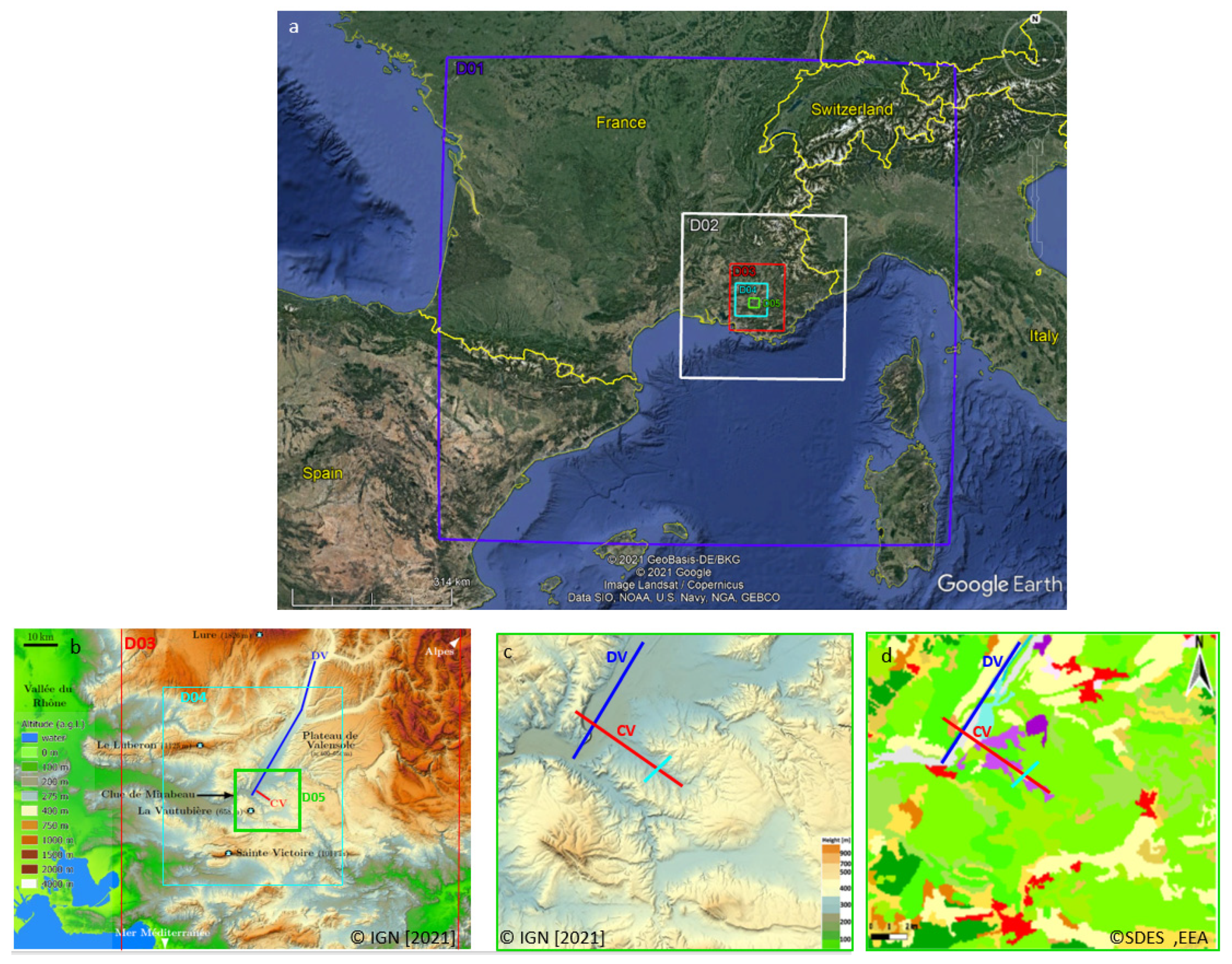
2.1. Location
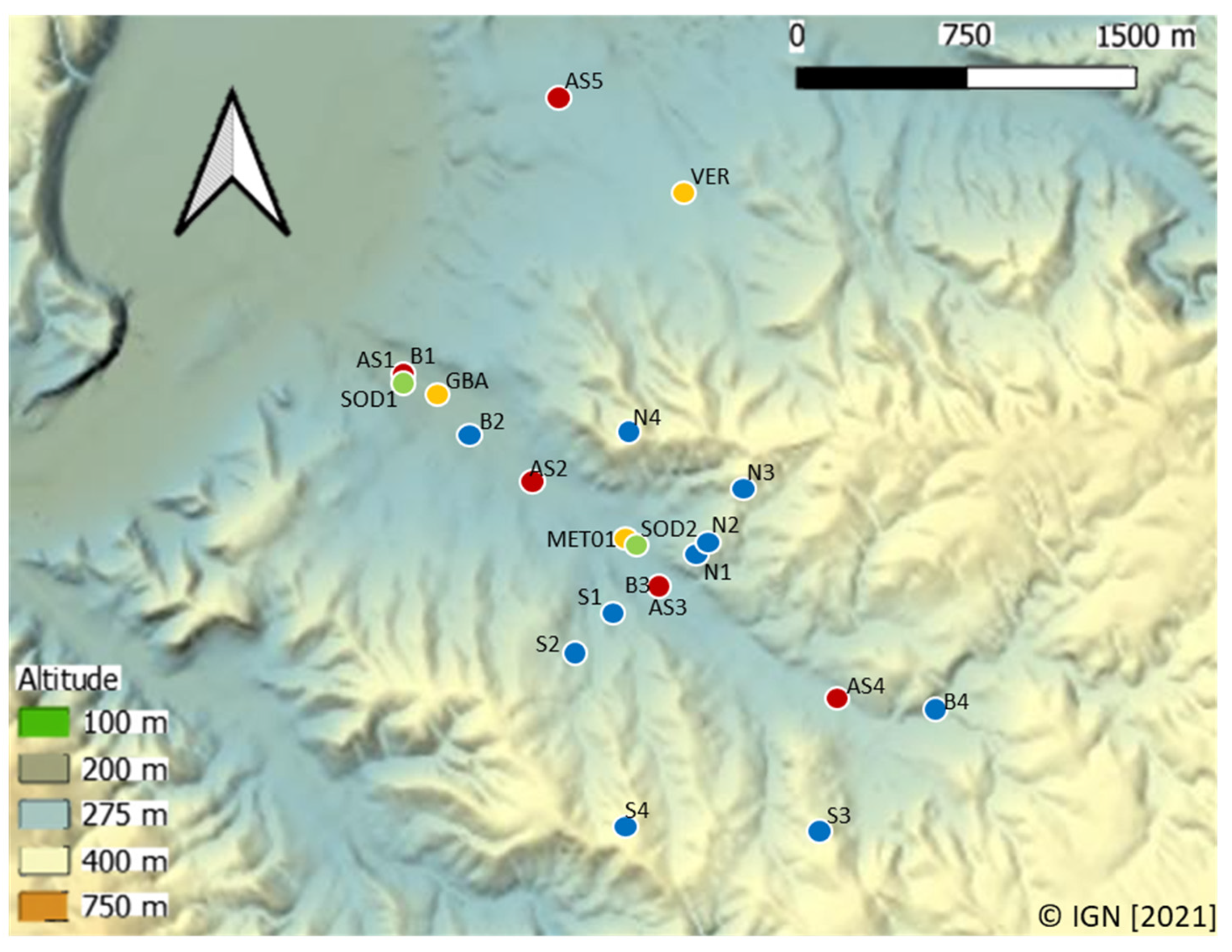
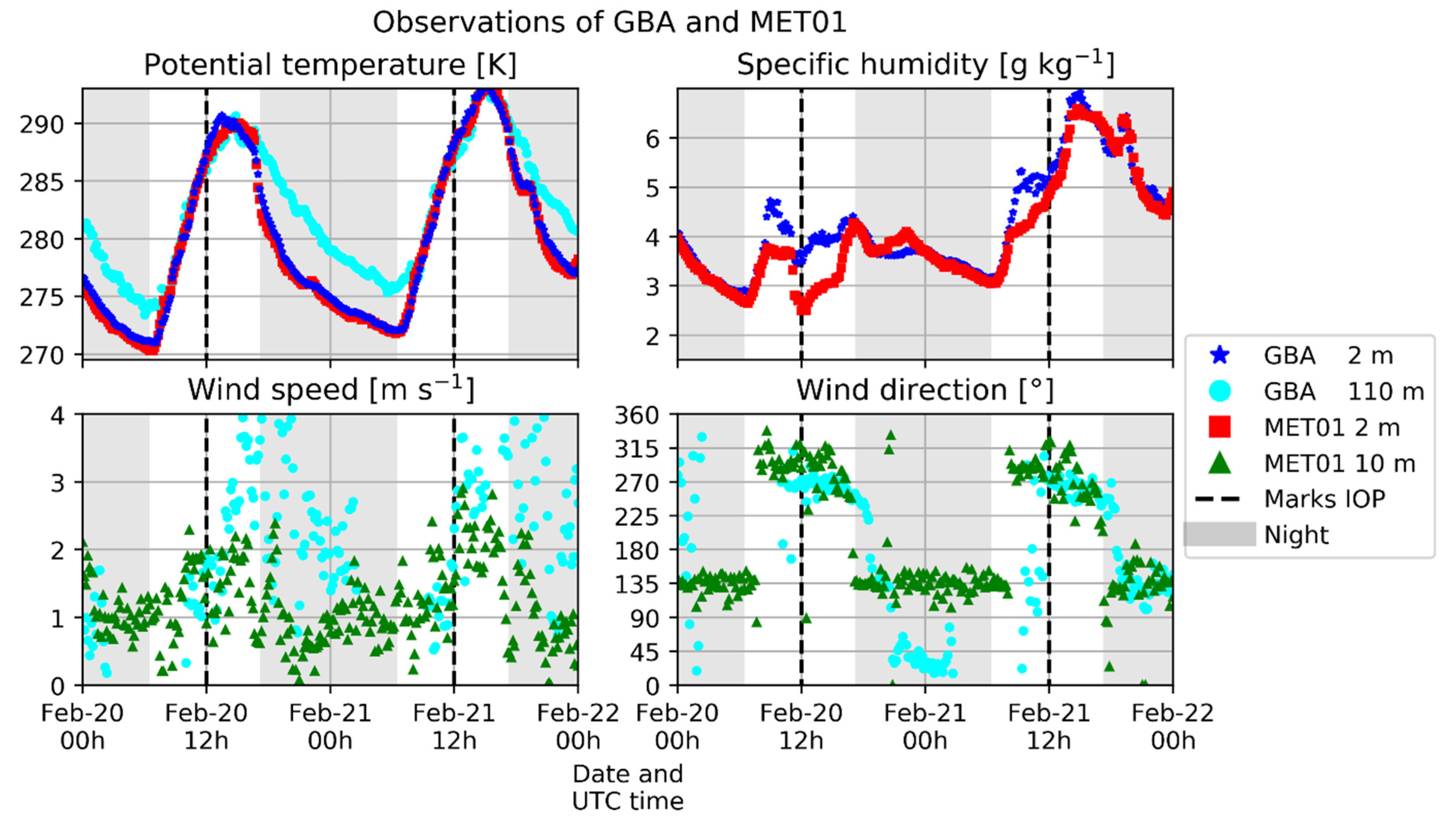
2.2. Observations
2.3. Selection and Characteristics of the Case Study
2.4. Configuration of the Numerical Simulation
2.4.1. Domain Settings
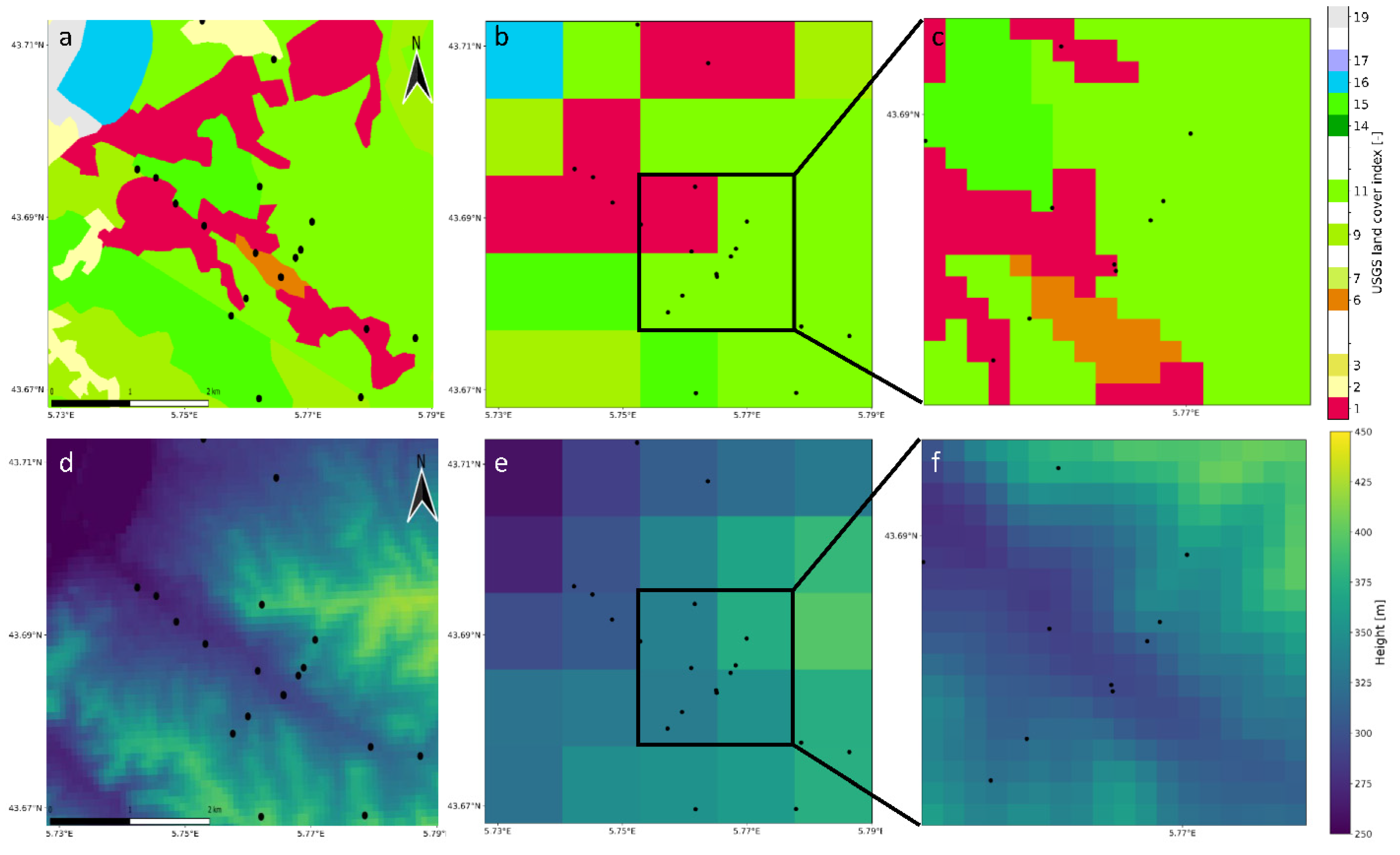
2.4.2. Representation of the Ground
2.5. Parameterizations
3. Results: Simulation vs. Observations
3.1. Improvement in the Refined Simulation
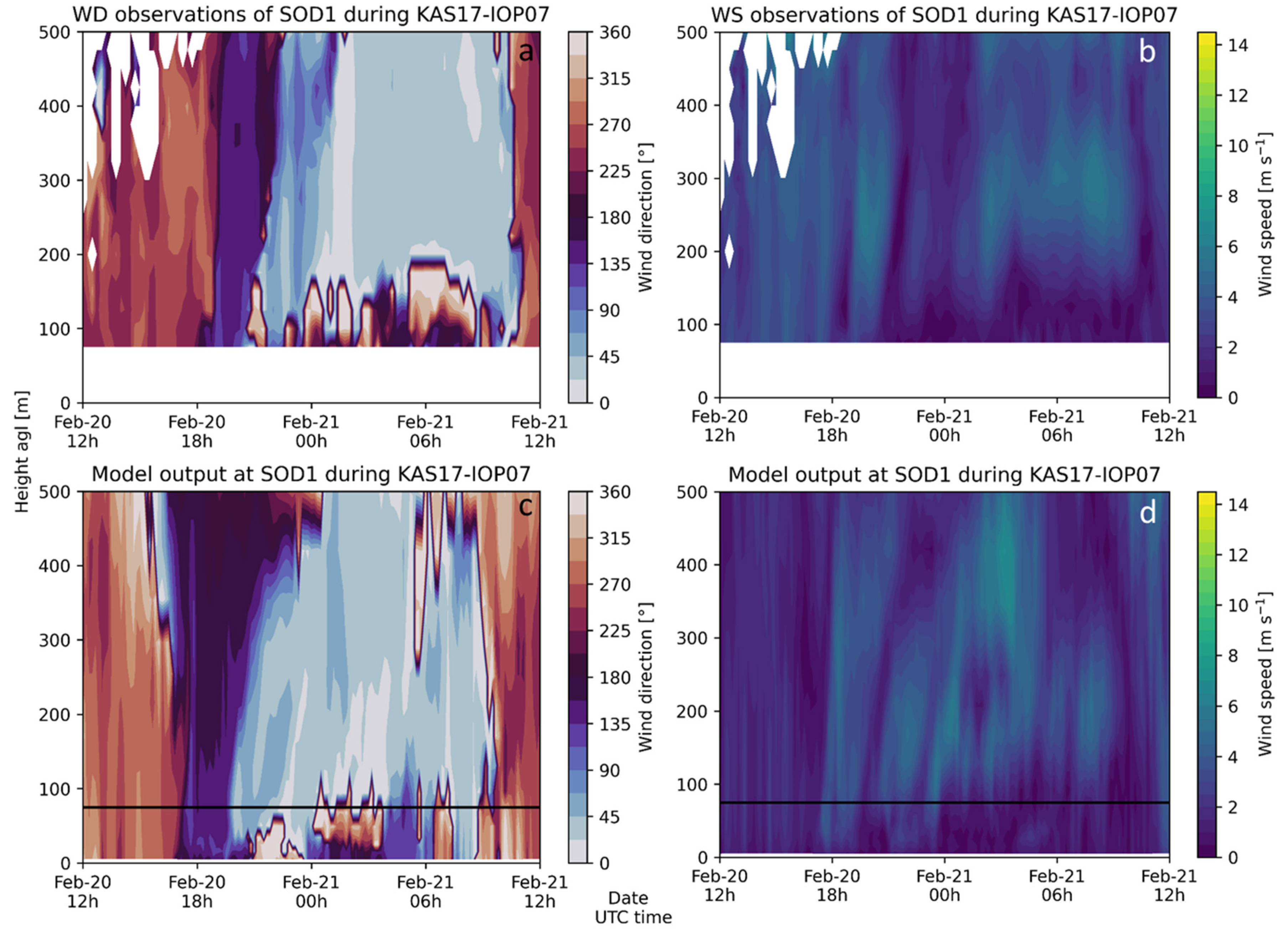
3.2. Overall Vertical Structure
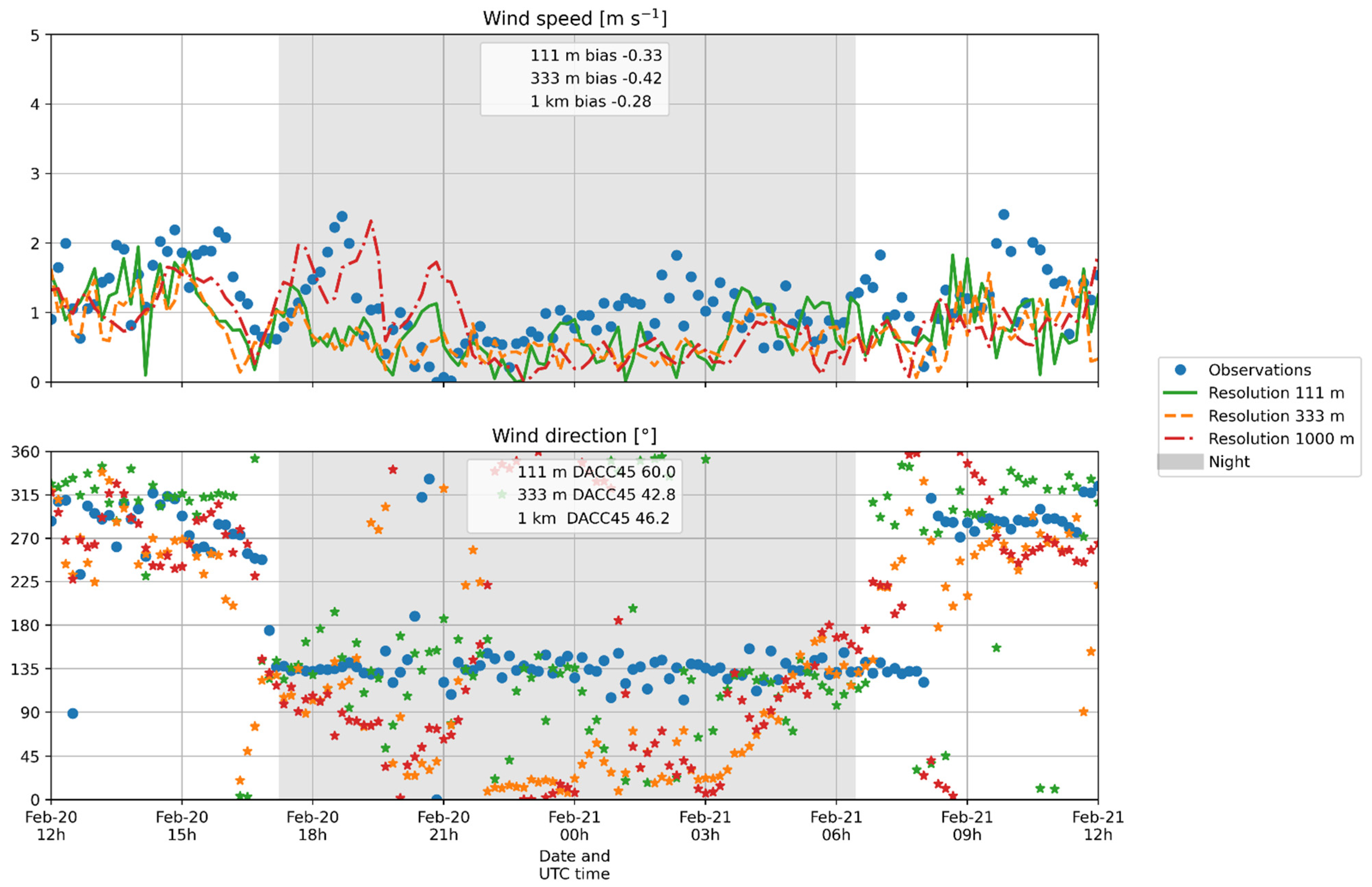
3.3. Diurnal Cycle
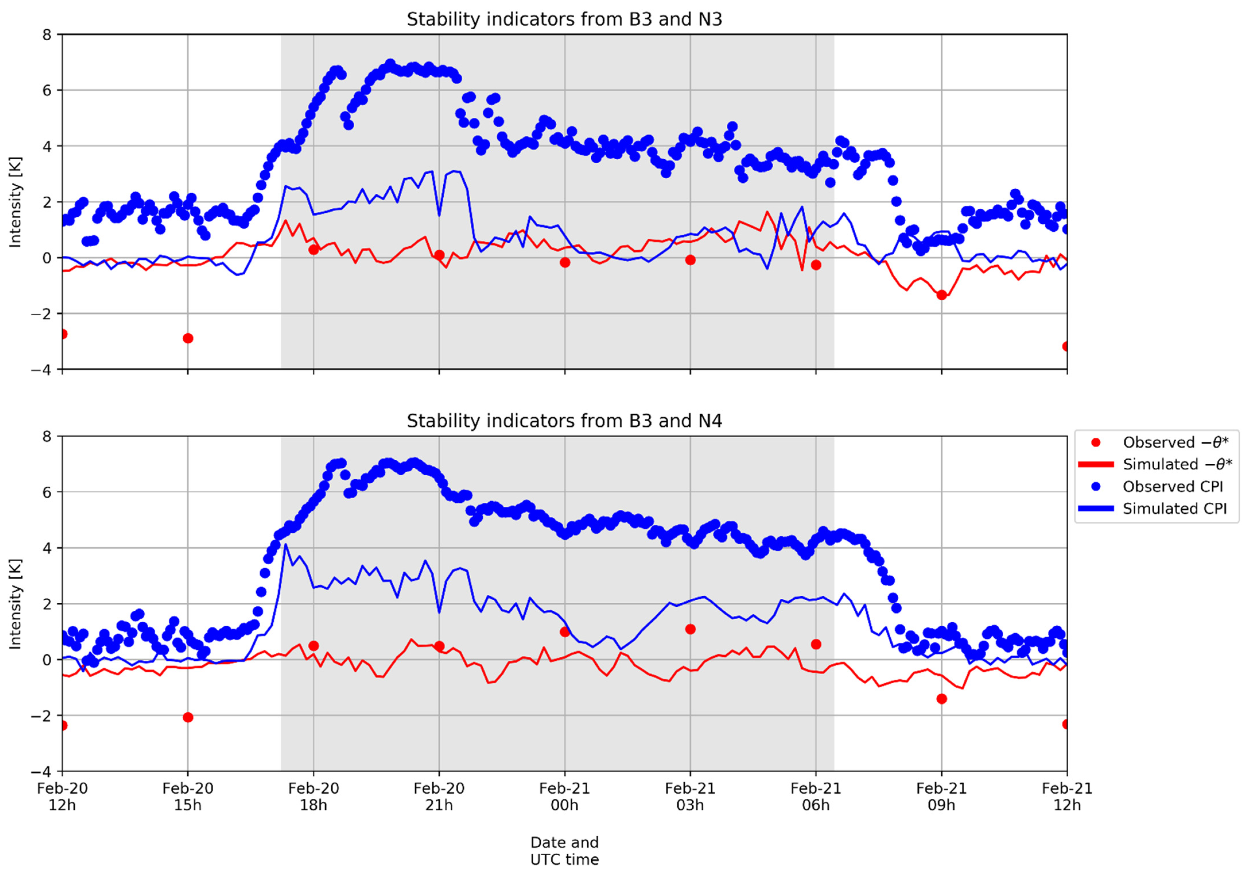
3.4. Simulation of the Stratification
- The cold pool intensity (CPI), which is the potential temperature difference between the top of the flank and the bottom of the valley;
- The potential temperature difference on a horizontal plane between the top of the flank and the center of the valley (θ*).
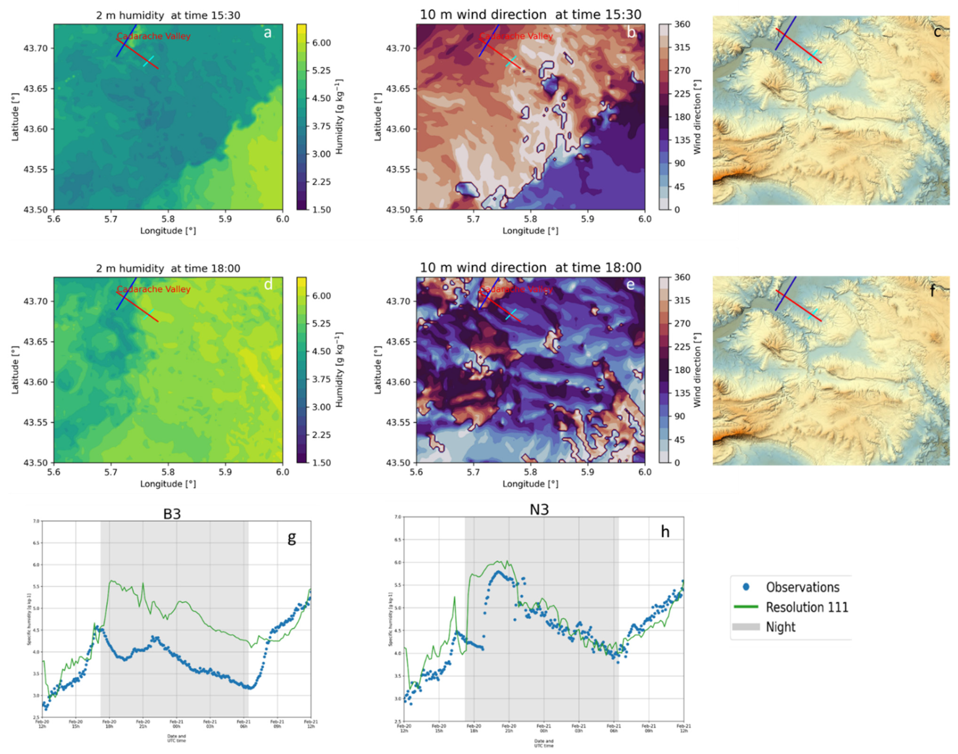
3.5. Moisture Fields
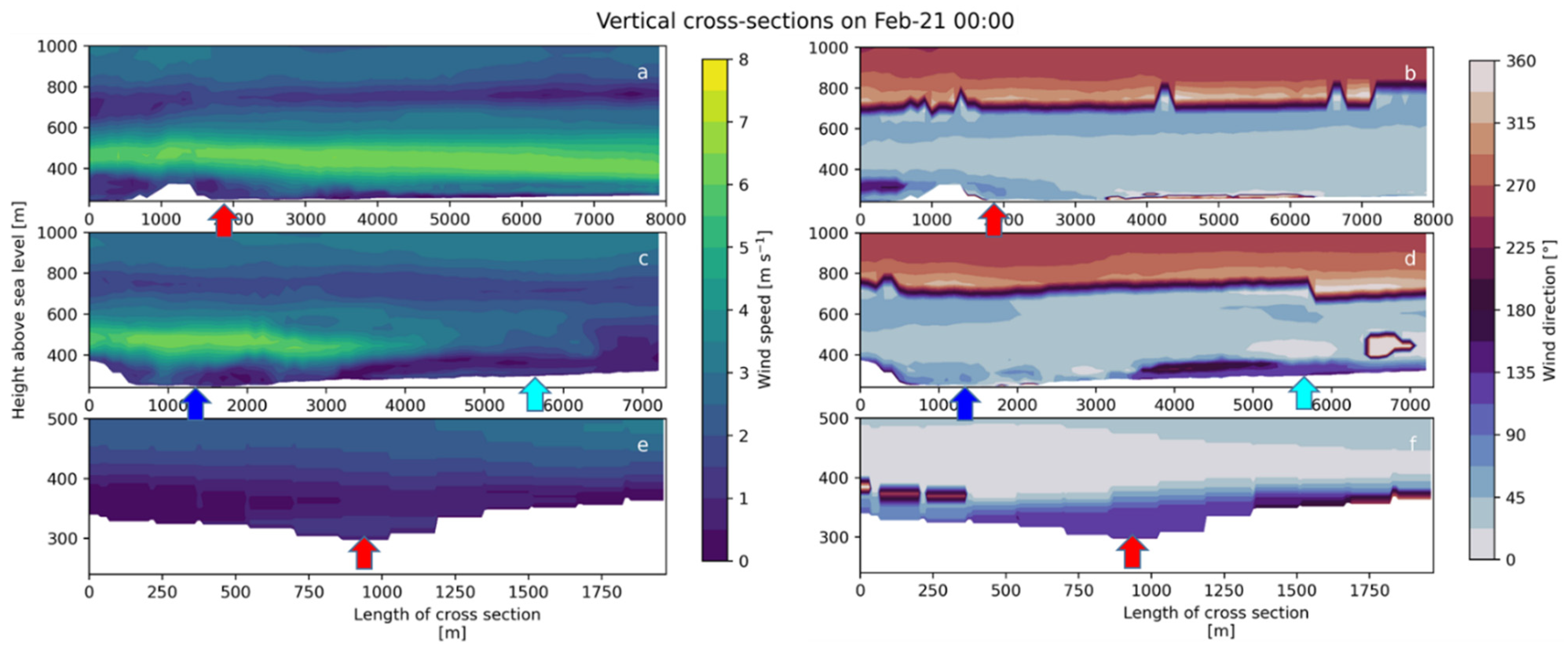
3.6. Vertical Cross-Sections
4. Discussion
4.1. Wind Modeling—Vertical Profiles
4.2. Stratification and Slope Flow
4.3. Moisture Field and Transport
4.4. Perspective
5. Conclusions
Author Contributions
Funding
Data Availability Statement
Conflicts of Interest
Appendix A

| Time of Radio-Sounding (UTC) | Start of 30 min w Time Series at 10 m (UTC) | Boundary Layer Height zi (m agl) | Integral Scale at 10 m from Spectra (m) | Integral Scale Extrapolated at zi with (A2) (m) | Integral Scale Computed at zi with (A1) (m) |
|---|---|---|---|---|---|
| 12:00 | 11:30 | 592 | 3.6 | 28 | 142 |
| 11:45 | 3.6 | 28 | |||
| 12:00 | 3.5 | 27 | |||
| 15:00 | 14:30 | 855 | 3.9 | 36 | 205 |
| 14:45 | 8.3 | 77 | |||
| 15:00 | 4.0 | 37 | |||
| 18:00 | 17:30 | 29 | 2.0 | 3 | 7 |
| 17:45 | 2.1 | 4 | |||
| 18:00 | 4.0 | 7 | |||
| 12:00 | 11:30 | 716 | 5.8 | 49 | 172 |
| 11:45 | 6.9 | 58 | |||
| 12:00 | 3.9 | 33 |

Appendix B
| Class Number | Full Name | Color |
|---|---|---|
| 1 | “Urban and Build-Up land” | |
| 2 | “Dryland Cropland and Pasture” | |
| 3 | “Irrigated Cropland and pastures” | |
| 6 | “Crops/Wood mosaic” | |
| 7 | “Grassland” | |
| 9 | “Mix Shrubland/Grassland” | |
| 11 | “Deciduous Broadleaf Forest” | |
| 14 | “Evergreen Needleleaf” | |
| 15 | “Mixed Forest” | |
| 16 | “Water Bodies” | |
| 17 | “Herbaceous Wetland” | |
| 19 | “Barren or Sparsely Vegetated” | |
| 24 | “Snow or Ice” |

References
- Sandu, I.; van Niekerk, A.; Shepherd, T.G.; Vosper, S.B.; Zadra, A.; Bacmeister, J.; Beljaars, A.; Brown, A.R.; Dörnbrack, A.; McFarlane, N.; et al. Impacts of Orography on Large-Scale Atmospheric Circulation. NPJ Clim. Atmos. Sci. 2019, 2, 1–8. [Google Scholar] [CrossRef]
- Lehner, M.; Whiteman, C.D.; Dorninger, M. Inversion Build-Up and Cold-Air Outflow in a Small Alpine Sinkhole. Bound.-Layer Meteorol. 2017, 163, 497–522. [Google Scholar] [CrossRef]
- Chemel, C.; Arduini, G.; Staquet, C.; Largeron, Y.; Legain, D.; Tzanos, D.; Paci, A. Valley Heat Deficit as a Bulk Measure of Wintertime Particulate Air Pollution in the Arve River Valley. Atmos. Environ. 2016, 128, 208–215. [Google Scholar] [CrossRef] [Green Version]
- Sabatier, T.; Paci, A.; Lac, C.; Canut, G.; Largeron, Y.; Masson, V. Semi-Idealized Simulations of Wintertime Flows and Pollutant Transport in an Alpine Valley: Origins of Local Circulations (Part I). Q. J. R. Meteorol. Soc. 2020, 146, 807–826. [Google Scholar] [CrossRef] [Green Version]
- Sabatier, T.; Largeron, Y.; Paci, A.; Lac, C.; Rodier, Q.; Canut, G.; Masson, V. Semi-Idealized Simulations of Wintertime Flows and Pollutant Transport in an Alpine Valley. Part II: Passive Tracer Tracking. Q. J. R. Meteorol. Soc. 2020, 146, 827–845. [Google Scholar] [CrossRef]
- Quimbayo-Duarte, J.; Staquet, C.; Chemel, C.; Arduini, G. Dispersion of Tracers in the Stable Atmosphere of a Valley Opening onto a Plain. Bound.-Layer Meteorol. 2019, 172, 291–315. [Google Scholar] [CrossRef]
- Quimbayo-Duarte, J.; Staquet, C.; Chemel, C.; Arduini, G. Impact of along-Valley Orographic Variations on the Dispersion of Passive Tracers in a Stable Atmosphere. Atmosphere 2019, 10, 225. [Google Scholar] [CrossRef] [Green Version]
- Doran, J.C.; Fast, J.D.; Horel, J. The Vtmx 2000 Campaign. Bull. Am. Meteorol. Soc. 2002, 83, 537–554. [Google Scholar] [CrossRef]
- Price, J.D.; Vosper, S.; Brown, A.; Ross, A.; Clark, P.; Davies, F.; Horlacher, V.; Claxton, B.; McGregor, J.R.; Hoare, J.S.; et al. COLPEX: Field and Numerical Studies over a Region of Small Hills. Bull. Am. Meteorol. Soc. 2011, 92, 1636–1650. [Google Scholar] [CrossRef] [Green Version]
- Whiteman, C.D.; Muschinski, A.; Zhong, S.; Fritts, D.; Hoch, S.W.; Hahnenberger, M.; Yao, W.; Hohreiter, V.; Behn, M.; Cheon, Y.; et al. Metcrax 2006: Meteorological Experiments in Arizona’s Meteor Crater. Bull. Am. Meteorol. Soc. 2008, 89, 1665–1680. [Google Scholar] [CrossRef] [Green Version]
- Fernando, H.J.S.; Pardyjak, E.R.; Sabatino, S.D.; Chow, F.K.; Wekker, S.F.J.D.; Hoch, S.W.; Hacker, J.; Pace, J.C.; Pratt, T.; Pu, Z.; et al. The MATERHORN: Unraveling the Intricacies of Mountain Weather. Bull. Am. Meteorol. Soc. 2015, 96, 1945–1967. [Google Scholar] [CrossRef]
- Clements, W.E.; Archuleta, J.A.; Gudiksen, P.H. Experimental Design of the 1984 ASCOT Field Study. J. Appl. Meteorol. Climatol. 1989, 28, 405–413. [Google Scholar] [CrossRef] [Green Version]
- Sabatier, T.; Paci, A.; Canut, G.; Largeron, Y.; Dabas, A.; Donier, J.-M.; Douffet, T. Wintertime Local Wind Dynamics from Scanning Doppler Lidar and Air Quality in the Arve River Valley. Atmosphere 2018, 9, 118. [Google Scholar] [CrossRef] [Green Version]
- Quimbayo-Duarte, J.; Chemel, C.; Staquet, C.; Troude, F.; Arduini, G. Drivers of Severe Air Pollution Events in a Deep Valley during Wintertime: A Case Study from the Arve River Valley, France. Atmos. Environ. 2021, 247, 118030. [Google Scholar] [CrossRef]
- Rotach, M.W.; Stiperski, I.; Fuhrer, O.; Goger, B.; Gohm, A.; Obleitner, F.; Rau, G.; Sfyri, E.; Vergeiner, J. Investigating Exchange Processes over Complex Topography: The Innsbruck Box (i-Box). Bull. Am. Meteorol. Soc. 2017, 98, 787–805. [Google Scholar] [CrossRef]
- Wagner, J.; Gerz, T.; Wildmann, N.; Gramitzky, K. Long-Term Simulation of the Boundary Layer Flow over the Double-Ridge Site during the Perdigão 2017 Field Campaign. Atmos. Chem. Phys. 2019, 19, 1129–1146. [Google Scholar] [CrossRef] [Green Version]
- Rotach, M.W.; Andretta, M.; Calanca, P.; Weigel, A.P.; Weiss, A. Boundary Layer Characteristics and Turbulent Exchange Mechanisms in Highly Complex Terrain. Acta Geophys. 2008, 56, 194–219. [Google Scholar] [CrossRef]
- Whiteman, C.D.; Allwine, K.J.; Fritschen, L.J.; Orgill, M.M.; Simpson, J.R. Deep Valley Radiation and Surface Energy Budget Microclimates. Part II: Energy Budget. J. Appl. Meteorol. Climatol. 1989, 28, 427–437. [Google Scholar] [CrossRef] [Green Version]
- Lehner, M.; Rotach, M.W.; Sfyri, E.; Obleitner, F. Spatial and Temporal Variations in Near-Surface Energy Fluxes in an Alpine Valley under Synoptically Undisturbed and Clear-Sky Conditions. Q. J. R. Meteorol. Soc. 2021, 147, 2173–2196. [Google Scholar] [CrossRef]
- Banakh, V.A.; Smalikho, I.N. Lidar Observations of Atmospheric Internal Waves in the Boundary Layer of the Atmosphere on the Coast of Lake Baikal. Atmos. Meas. Tech. 2016, 9, 5239–5248. [Google Scholar] [CrossRef] [Green Version]
- Duine, G.-J.; Hedde, T.; Roubin, P.; Durand, P.; Lothon, M.; Lohou, F.; Augustin, P.; Fourmentin, M. Characterization of Valley Flows within Two Confluent Valleys under Stable Conditions: Observations from the KASCADE Field Experiment. Q. J. R. Meteorol. Soc. 2017, 143, 1886–1902. [Google Scholar] [CrossRef] [Green Version]
- Dupuy, F. Amélioration de la Connaissance et de la Prévision des Vents de Vallée en Conditions Stables: Expérimentation et Modélisation Statistique Avec Réseau de Neurones Artificiels. Ph.D. Thesis, Université de Toulouse, Université Toulouse III-Paul Sabatier, Toulouse, France, 2019. [Google Scholar]
- Duine, G.-J.; Hedde, T.; Roubin, P.; Durand, P. A Simple Method Based on Routine Observations to Nowcast Down-Valley Flows in Shallow, Narrow Valleys. J. Appl. Meteor. Climatol. 2016, 55, 1497–1511. [Google Scholar] [CrossRef]
- Dupuy, F.; Duine, G.-J.; Durand, P.; Hedde, T.; Roubin, P.; Pardyjak, E. Local-Scale Valley Wind Retrieval Using an Artificial Neural Network Applied to Routine Weather Observations. J. Appl. Meteorol. Climatol. 2019, 58, 1007–1022. [Google Scholar] [CrossRef] [Green Version]
- Dupuy, F.; Duine, G.-J.; Durand, P.; Hedde, T.; Pardyjak, E.; Roubin, P. Valley Winds at the Local Scale: Correcting Routine Weather Forecast Using Artificial Neural Networks. Atmosphere 2021, 12, 128. [Google Scholar] [CrossRef]
- Goger, B.; Rotach, M.W.; Gohm, A.; Fuhrer, O.; Stiperski, I.; Holtslag, A.A.M. The Impact of Three-Dimensional Effects on the Simulation of Turbulence Kinetic Energy in a Major Alpine Valley. Bound.-Layer Meteorol. 2018, 168, 1–27. [Google Scholar] [CrossRef] [Green Version]
- Udina, M.; Sun, J.; Kosović, B.; Soler, M.R. Exploring Vertical Turbulence Structure in Neutrally and Stably Stratified Flows Using the Weather Research and Forecasting–Large-Eddy Simulation (WRF–LES) Model. Bound.-Layer Meteorol. 2016, 161, 355–374. [Google Scholar] [CrossRef]
- Jemmett-Smith, B.C.; Ross, A.N.; Sheridan, P.F.; Hughes, J.K.; Vosper, S.B. A Case-Study of Cold-Air Pool Evolution in Hilly Terrain Using Field Measurements from COLPEX. Q. J. R. Meteorol. Soc. 2019, 145, 1290–1306. [Google Scholar] [CrossRef] [Green Version]
- Skamarock, C.; Klemp, B.; Dudhia, J.; Gill, O.; Liu, Z.; Berner, J.; Wang, W.; Powers, G.; Duda, G.; Barker, D.; et al. A Description of the Advanced Research WRF Model Version 4. Natl. Cent. Atmos. Res. 2019, 145. [Google Scholar] [CrossRef]
- Skamarock, W.C.; Klemp, J.B.; Dudhia, J.; Gill, D.O.; Barker, D.M.; Duda, M.G.; Huang, X.-Y.; Wang, W.; Powers, J.G. A Description of the Advanced Research WRF Version 3, NCAR/TN-475+STR; National Center for Atmospheric Research (NCAR): Boulder, CO, USA, 2008; 113p. [Google Scholar]
- Kalverla, P.C.; Duine, G.-J.; Steeneveld, G.-J.; Hedde, T. Evaluation of the Weather Research and Forecasting Model in the Durance Valley Complex Terrain during the KASCADE Field Campaign. J. Appl. Meteor. Climatol. 2016, 55, 861–882. [Google Scholar] [CrossRef]
- Bastin, S.; Drobinski, P.; Dabas, A.; Delville, P.; Reitebuch, O.; Werner, C. Impact of the Rhône and Durance Valleys on Sea-Breeze Circulation in the Marseille Area. Atmos. Res. 2005, 74, 303–328. [Google Scholar] [CrossRef]
- Gunawardena, N.; Pardyjak, E.R.; Stoll, R.; Khadka, A. Development and Evaluation of an Open-Source, Low-Cost Distributed Sensor Network for Environmental Monitoring Applications. Meas. Sci. Technol. 2018, 29, 024008. [Google Scholar] [CrossRef]
- Wang, W.; Gill, D. WRF Nesting. WRF tutorial 2012 Brazil; University of Sao Paulo: Sao Paulo, Brazil, 2012. [Google Scholar]
- Daniels, M.H.; Lundquist, K.A.; Mirocha, J.D.; Wiersema, D.J.; Chow, F.K. A New Vertical Grid Nesting Capability in the Weather Research and Forecasting (WRF) Model. Mon. Weather. Rev. 2016, 144, 3725–3747. [Google Scholar] [CrossRef]
- Duine, G.-J. Caractérisation Des Vents de Vallée En Conditions Stables à Partir de La Campagne de Mesures KASCADE et de Simulations WRF à Méso-Échelle. Ph.D. Thesis, Université de Toulouse, Université Toulouse III-Paul Sabatier, Toulouse, France, 2015. [Google Scholar]
- Hersbach, H.; Bell, B.; Berrisford, P.; Biavati, G.; Horányi, A.; Muñoz Sabater, J.; Nicolas, J.; Peubey, C.; Radu, R.; Rozum, I.; et al. ERA5 Hourly Data on Pressure Levels from 1978 to Present, Copernicus Climate Change Service (C3S) Climate Data Store (CDS). 2018. Available online: https://cds.climate.copernicus.eu/cdsapp#!/dataset/reanalysis-era5-pressure-levels?tab=overview (accessed on 10 August 2021). [CrossRef]
- Hersbach, H.; Bell, B.; Berrisford, P.; Biavati, G.; Horányi, A.; Muñoz Sabater, J.; Nicolas, J.; Peubey, C.; Radu, R.; Rozum, I.; et al. ERA5 Hourly Data on Model Level from 1978 to Present, Copernicus Climate Change Service (C3S) Climate Data Store (CDS). 2018. Available online: https://cds.climate.copernicus.eu/cdsapp#!/dataset/reanalysis-era5-single-levels?tab=overview (accessed on 10 August 2021). [CrossRef]
- Hong, S.-Y.; Kim, J.-H.; Lim, J.; Dudhia, J. The WRF Single Moment Microphysics Scheme (WSM). J. Korean Meteorol. Soc. 2006, 42, 129–151. [Google Scholar]
- Sukoriansky, S.; Galperin, B.; Perov, V. Application of a New Spectral Theory of Stably Stratified Turbulence to the Atmospheric Boundary Layer over Sea Ice. Bound.-Layer Meteorol. 2005, 117, 231–257. [Google Scholar] [CrossRef]
- Kain, J.S. The Kain–Fritsch Convective Parameterization: An Update. J. Appl. Meteorol. Climatol. 2004, 43, 170–181. [Google Scholar] [CrossRef] [Green Version]
- Sukoriansky, S. Implementation of the Quasi-Normal Scale Elimination (QNSE) Model of Stably Stratified Turbulence in WRF; Report on WRF-DTC Visit of Semion Sukoriansky; Ben Gurion University of the Negev: Beer-Sheva, Israel, 2008; 8p. [Google Scholar]
- Iacono, M.J.; Delamere, J.S.; Mlawer, E.J.; Shephard, M.W.; Clough, S.A.; Collins, W.D. Radiative Forcing by Long-Lived Greenhouse Gases: Calculations with the AER Radiative Transfer Models. J. Geophys. Res. Atmos. 2008, 113. [Google Scholar] [CrossRef]
- Tewari, M.; Chen, F.; Wang, W.; Dudhia, J.; LeMone, M.; Mitchell, K.; Ek, M.; Gayno, G.; Wegiel, J. Implementation and Verification of the Unified NOAH Land Surface Model in the WRF Model (Formerly Paper Number 17.5). In Proceedings of the 20th Conference on Weather Analysis and Forecasting/16th Conference on Numerical Weather Prediction, Seattle, WA, USA, 14 January 2004; pp. 11–15. [Google Scholar]
- Farr, T.G.; Kobrick, M. Shuttle Radar Topography Mission Produces a Wealth of Data. Eos Trans. Am. Geophys. Union 2000, 81, 583–585. [Google Scholar] [CrossRef]
- Mukul, M.; Srivastava, V.; Mukul, M. Accuracy Analysis of the 2014–2015 Global Shuttle Radar Topography Mission (SRTM) 1 Arc-Sec C-Band Height Model Using International Global Navigation Satellite System Service (IGS) Network. J. Earth Syst. Sci. 2016, 125, 909–917. [Google Scholar] [CrossRef] [Green Version]
- Pineda, N.; Jorba, O.; Jorge, J.; Baldasano, J.M. Using NOAA AVHRR and SPOT VGT Data to Estimate Surface Parameters: Application to a Mesoscale Meteorological Model. Int. J. Remote Sens. 2004, 25, 129–143. [Google Scholar] [CrossRef]
- Vladimirov, E.; Dimitrova, R.; Danchovski, V. Sensitivity of WRF Model Results to Topography and Land Cover: Study for the Sofia Region. Annu. Univ. Sofia St. Kliment Ohridski 2018, 111, 87–101. [Google Scholar]
- Egova, E.; Dimitrova, R.; Danchovski, V. Numerical Study of Meso-Scale Circulation Specifics in the Sofia. Bul. J. Meteorol. Hydrol. 2017, 22, 54–72. [Google Scholar]
- Wyngaard, J.C. Toward Numerical Modeling in the “Terra Incognita”. J. Atmos. Sci. 2004, 61, 1816–1826. [Google Scholar] [CrossRef]
- Kaimal, J.C.; Finnigan, J.J. Atmospheric Boundary Layer Flows: Their Structure and Measurement; Oxford University Press: Oxford, UK, 1994; ISBN 978-0-19-536277-0. [Google Scholar]
- Lenschow, D.H.; Stankov, B.B. Length Scales in the Convective Boundary Layer. J. Atmos. Sci. 1986, 43, 1198–1209. [Google Scholar] [CrossRef]
- Zhang, X.; Bao, J.-W.; Chen, B.; Grell, E.D. A Three-Dimensional Scale-Adaptive Turbulent Kinetic Energy Scheme in the WRF-ARW Model. Mon. Weather. Rev. 2018, 146, 2023–2045. [Google Scholar] [CrossRef]
- Deardorff, J.W. Stratocumulus-Capped Mixed Layers Derived from a Three-Dimensional Model. Bound.-Layer Meteorol. 1980, 18, 495–527. [Google Scholar] [CrossRef]
- Weisman, M.L.; Skamarock, W.C.; Klemp, J.B. The Resolution Dependence of Explicitly Modeled Convective Systems. Mon. Weather. Rev. 1997, 125, 527–548. [Google Scholar] [CrossRef]
- Jeworrek, J.; West, G.; Stull, R. Evaluation of Cumulus and Microphysics Parameterizations in WRF across the Convective Gray Zone. Weather. Forecast. 2019, 34, 1097–1115. [Google Scholar] [CrossRef]
- Mahoney, K.M. The Representation of Cumulus Convection in High-Resolution Simulations of the 2013 Colorado Front Range Flood. Mon. Weather. Rev. 2016, 144, 4265–4278. [Google Scholar] [CrossRef]
- Lindvall, J.; Svensson, G. The Diurnal Temperature Range in the CMIP5 Models. Clim. Dyn. 2015, 44, 405–421. [Google Scholar] [CrossRef]
- Acevedo, O.C.; Fitzjarrald, D.R. The Early Evening Surface-Layer Transition: Temporal and Spatial Variability. J. Atmos. Sci. 2001, 58, 2650–2667. [Google Scholar] [CrossRef]
- Blumberg, W.G.; Turner, D.D.; Cavallo, S.M.; Gao, J.; Basara, J.; Shapiro, A. An Analysis of the Processes Affecting Rapid Near-Surface Water Vapor Increases during the Afternoon to Evening Transition in Oklahoma. J. Appl. Meteorol. Climatol. 2019, 58, 2217–2234. [Google Scholar] [CrossRef]
- Mahrt, L. Stably Stratified Flow in a Shallow Valley. Bound.-Layer Meteorol. 2017, 162, 1–20. [Google Scholar] [CrossRef]
- Jiménez, M.A.; Cuxart, J.; Martínez-Villagrasa, D. Influence of a Valley Exit Jet on the Nocturnal Atmospheric Boundary Layer at the Foothills of the Pyrenees. Q. J. R. Meteorol. Soc. 2019, 145, 356–375. [Google Scholar] [CrossRef] [Green Version]
- Albergel, C.; de Rosnay, P.; Gruhier, C.; Muñoz-Sabater, J.; Hasenauer, S.; Isaksen, L.; Kerr, Y.; Wagner, W. Evaluation of Remotely Sensed and Modelled Soil Moisture Products Using Global Ground-Based in Situ Observations. Remote. Sens. Environ. 2012, 118, 215–226. [Google Scholar] [CrossRef]
- Durand, P.; Thoumieux, F.; Lambert, D. Turbulent Length-Scales in the Marine Atmospheric Mixed Layer. Q. J. R. Meteorol. Soc. 2000, 126, 1889–1912. [Google Scholar] [CrossRef]
- Darbieu, C.; Lohou, F.; Lothon, M.; Vilà-Guerau de Arellano, J.; Couvreux, F.; Durand, P.; Pino, D.; Patton, E.G.; Nilsson, E.; Blay-Carreras, E.; et al. Turbulence Vertical Structure of the Boundary Layer during the Afternoon Transition. Atmos. Chem. Phys. 2015, 15, 10071–10086. [Google Scholar] [CrossRef] [Green Version]
- Brilouet, P.-E.; Durand, P.; Canut, G. The Marine Atmospheric Boundary Layer under Strong Wind Conditions: Organized Turbulence Structure and Flux Estimates by Airborne Measurements. J. Geophys. Res. Atmos. 2017, 122, 2115–2130. [Google Scholar] [CrossRef]
- Kristensen, L.; Lenschow, D.H.; Kirkegaard, P.; Courtney, M. The Spectral Velocity Tensor for Homogeneous Boundary-Layer Turbulence. Bound.-Layer Meteorol. 1989, 47, 149–193. [Google Scholar] [CrossRef]
- Kovadlo, P.G.; Shihovtsev, A.Y. The Study of Turbulence and Optical Instability in Stably Stratified Earth’s Atmosphere. In Proceedings of the 21st International Symposium Atmospheric and Ocean Optics: Atmospheric Physics, International Society for Optics and Photonics. Tomsk, Russian Federation, 19 November 2015; Volume 9680, p. 968074. [Google Scholar]


| Date | 2017-02-20 12:00:00 to 2017-02-21 12:00:00 | ||||
|---|---|---|---|---|---|
| WRF version | V 4.2 | ||||
| Global data forcing | ECMWF ERA5 1 h time step, 0.25° horizontal resolution, 38 vertical levels [37,38] | ||||
| Nesting | Two-way | ||||
| Vertical levels | 46 | ||||
| Simulation time (h) | 36 | ||||
| Spin-up (h) | 12 | ||||
| Top of model (hPa) | 50 | ||||
| Domain | D1 | D2 | D3 | D4 | D5 |
| Horizontal resolution (m) | 9000 | 3000 | 1000 | 333.333 | 111.111 |
| Number of cells | 106,100 | 100,100 | 100,121 | 175,178 | 169,154 |
| Topography map resolution | 5′ | 2′ | 30″ | 15″ | 3″ |
| Time step (s) | 45 | 15 | 5 | 0.5 | 0.125 |
| Output interval (min) | 180 | 180 | 10 | 10 | 10 |
| Parameterizations | |||||
| Microphysics | WRF single-moment 6-class scheme [39] | ||||
| Planetary boundary layer | Quasi-normal scale elimination (QNSE) scheme [40] | ||||
| Cumulus parametrization | Kain Fritsch [41] | ||||
| Surface layer | QNSE surface layer unified [42] | ||||
| Longwave radiation | RRTMG [43] | ||||
| Shortwave radiation | RRTMG [43] | ||||
| Land surface option | NOAH land surface model [44] | ||||
Publisher’s Note: MDPI stays neutral with regard to jurisdictional claims in published maps and institutional affiliations. |
© 2021 by the authors. Licensee MDPI, Basel, Switzerland. This article is an open access article distributed under the terms and conditions of the Creative Commons Attribution (CC BY) license (https://creativecommons.org/licenses/by/4.0/).
Share and Cite
de Bode, M.; Hedde, T.; Roubin, P.; Durand, P. Fine-Resolution WRF Simulation of Stably Stratified Flows in Shallow Pre-Alpine Valleys: A Case Study of the KASCADE-2017 Campaign. Atmosphere 2021, 12, 1063. https://0-doi-org.brum.beds.ac.uk/10.3390/atmos12081063
de Bode M, Hedde T, Roubin P, Durand P. Fine-Resolution WRF Simulation of Stably Stratified Flows in Shallow Pre-Alpine Valleys: A Case Study of the KASCADE-2017 Campaign. Atmosphere. 2021; 12(8):1063. https://0-doi-org.brum.beds.ac.uk/10.3390/atmos12081063
Chicago/Turabian Stylede Bode, Michiel, Thierry Hedde, Pierre Roubin, and Pierre Durand. 2021. "Fine-Resolution WRF Simulation of Stably Stratified Flows in Shallow Pre-Alpine Valleys: A Case Study of the KASCADE-2017 Campaign" Atmosphere 12, no. 8: 1063. https://0-doi-org.brum.beds.ac.uk/10.3390/atmos12081063