A Global Empirical Model of the Ion Temperature in the Ionosphere for the International Reference Ionosphere

Abstract

This study presents a suggestion for improvement of the ion temperature (Ti) model in the International Reference Ionosphere (IRI). We have re-examined ion temperature data (primarily available from NASA’s Space Physics Data Facility (SPDF)from older satellites and combined them with newly available data from the Defense Meteorological Satellite Program (DMSP), the Communication Navigation Outage Forecasting System (C/NOFS), and from the recently launched Ionospheric Connection Explorer (ICON). We have compiled these data into a unified database comprising in total Ti data from 18 satellites. By comparisons with long term records of ion temperature from the three incoherent scatter radars (ISRs) (Jicamarca, Arecibo, and Millstone Hill), it was found that an intercalibration is needed to achieve consistency with the ISR data and among individual satellite data sets. This database with thus corrected data has been used for the development of a new global empirical model of Ti with inclusion of solar activity variation. This solar activity dependence is represented by an additive correction term to the Ti global pattern. Due to the limited data coverage at altitudes above 1000 km, the altitude range described by the model ranges from 350 km to 850 km covering only the region where generally Ti is higher than the neutral temperature (Tn) and lower than the electron temperature (Te). This approach is consistent with the current description of Ti in the IRI model. However, instead of one anchor point at 430 km altitude as in the current IRI, our approach includes anchor points at 350, 430, 600, and 850 km. At altitudes above 850 km Ti is merged using a gradient derived from the model at 600 and 850 km, with the electron temperature described by the IRI-2016/TBT-2012 option. Comparisons with the ISR data (Jicamarca, Arecibo, Millstone Hill, and Kharkiv) for high and low solar activity and equinox show that the proposed Ti model captures local time variation of Ti at different altitudes and latitudes better than the current IRI-2016 Ti model.

1. Introduction

The research on the temperatures of charged thermal particles, which is crucial for understanding thermal processes in the ionosphere and adjacent regions, has been conducted since the 1960s. As the understanding of these processes advanced, it was found that the ionospheric plasma is not in thermal equilibrium and, in general, the temperatures of the electrons (Te) and ions (Ti) are different [1]. Together with theoretical and experimental studies, the need for an empirical description of these temperatures emerged. The empirical description of Te and Ti in the ionosphere, topside ionosphere and plasmasphere is one of the tasks of the IRI COSPAR/URSI working group. The main efforts have been devoted to the modelling of the electron temperature (e.g., [2,3,4,5]), because the excess energy from the photoionization of neutral particles in the upper atmosphere by the solar EUV (Extreme ultraviolet) photons is primarily received by the electrons and then transferred to the ions and from them to the neutral particles, e.g., Schunk and Nagy [6]. Another reason for focusing on global empirical modeling of the electron temperature rather than the ion temperature was the relative simplicity of Te measurements with Langmuir probes [7] while ion temperature measurements required the more involved the retarding potential analyzers (RPA) technique [8] and more recently ion imagers [9]. As a result, the amount of data collected for the electron temperature far exceeded the amount of reliable ion temperature measurements [10].

The general formulation of the thermal balance equations includes temperatures related to different ion species, and thus in general different ions do not have the same temperature [11], which has also been pointed out experimentally in the case of the temperatures of light ions such as H⁺ versus heavier ones such as O⁺ [12]. Our study is focused on the O⁺ temperature since O⁺ is the predominant ion or constitutes a substantial fraction in the altitude range that is of interest for this study.

For the calculation of the ion temperature, the IRI model [13] employs an approach that is described in [14] (pp. 68–69) and was recently reviewed and assessed by Pignalberi et al. [15] with the help of the Millstone Hill incoherent scatter radar (ISR) data. The essence of this approach is that the model uses Ti RPA data from the AEROS-A satellite at an altitude of 430 km to establish a fixed anchor point at this altitude. Ti below this altitude is then extrapolated by searching for a tangential point on the neutral temperature (Tn) profile from the NRLMSISE-00 model [16]. Above 430 km altitude, an extrapolation is performed using the average gradient for day and night estimated using ISR data (Arecibo and Millstone Hill). The constraint $\mathrm{Tn}\le \mathrm{Ti}\le \mathrm{Te}$then applies in the whole range of altitudes. However, since the construction of this Ti model for IRI, an incomparably larger amount of Ti data has been accumulated and has become available through NASA’s Space Physics Data Facility (SPDF: https://spdf.gsfc.nasa.gov/pub/data, accessed on 7 November 2019) and through other data centers. Still, not all data are available, but the much more favorable policy of many universities and research institutions in sharing new data compared to the past allows more data to be collected for model construction. This has provided us with a large amount of data that we believe is suitable for revising the IRI Timodel and producing a new version, with the inclusion of more anchor points, better resolution in latitude and local time, and the explicit representation of variation with solar activity. Furthermore, we use the large volume of ISR data, that are publicly available thanks to the Open Madrigal Initiative (https://openmadrigal.org, accessed on 13 May 2020), for correction or intercalibration of the satellite data. Our study is a good example of the synergy obtained by combining data from different sources. Nevertheless, the model still has a number of limitations, and in the future it is necessary to obtain additional data or to engage other modelling techniques and methods in order to construct a model for the whole range of heights, including the incorporation of all relevant geophysical and solar parameters.

The paper is organized as follows. In Section 2, we describe our database, its verification, correction and intercalibration using ISR data. In Section 3, we present the construction of the proposed Ti model. Then, in Section 4, we describe how the altitude profiles were constructed and how they are connected to Tn and Te. In Section 5 we show the results of the model, and in Section 6 we compare with the ISR data. Finally, in Section 7 we discuss the findings and conclude the paper.

2. Data

We have built a database that comprises of as much available Ti data from in situ satellite measurements as possible. This database covers a time period of more than fifty years, i.e., almost five solar cycles.

Table 1. A list of the satellites and experiments included in the database and their corresponding time intervals, altitude, latitude, and solar local time (SLT) ranges, and the average PF10.7 index.

No	Satellite (Experiment)	Time Period (Data Avail)	Altitude [km]	Latitude [deg]	SLT [h]	$\overline{\mathit{P}\mathit{F}10.7}$
1	OGO-6 (RPA)	12. 1969–4. 1971	390–1090	−82 .. +82	0–24	155
2	AEROS A (RPA)	1. 1973–8. 1973	200–870	−83 .. +83	3, 15 fixed	98
3	AEROS B (RPA)	7. 1974–9. 1975	140–880	−83 .. +83	4, 16 fixed	86
4	AE-C (RPA)	12. 1973–12. 1978	135–2010	−68 .. +68	0–24	86
5	AE-D (RPA)	10. 1975–1. 1976	140–1980	−89 .. +89	0–24	76
6	AE-E (RPA)	12. 1975–5. 1981	140–1580	−20 .. +20	0–24	129
7	DE-2 (RPA)	8. 1981–2. 1983	200–1020	−90 .. +90	0–24	180
8	San Marco 5 (RPA)	4. 1988–12. 1988	170–590	−3 .. +3	0–24	151
9	IK24 (RPA)	10. 1989–2. 1993	500–2525	−83 .. +84	0–24	195
10	DMSP F11 (RPA)	1. 1992–5. 2000	840–890	−81 .. +87	6, 18 fixed	119
11	DMSP F12 (RPA)	1. 1996–6. 2002	840–890	−82 .. +89	9, 21 fixed	132
12	DMSP F13 (RPA)	3. 1995–12. 2005	840–880	−81 .. +82	6, 18 fixed	131
13	DMSP F14 (RPA)	4. 1997–7. 2003	840–885	−81 .. +82	9, 21 fixed	121
14	DMSP F15 (RPA)	12. 1999–12. 2017	830–880	−86 .. +86	9.5, 21.5 fixed	116
15	SROSS C2 (RPA)	1. 1995–12. 2000	380–620	−40 .. +45	0–24	110
16	ROCSAT-1(RPA)	3. 1999–6. 2004	560–665	−35 .. +35	0–24	160
17	C/NOFS (RPA)	8. 2008–11. 2015	260–855	−13 .. +13	0–24	106
18	ICON IVM (RPA)	10. 2019–6. 2020	575–610	−27 .. 27	0–24	70

Relevant references to the experiments onboard individual satellites: (1) Hanson et al. [18]; (2, 3) Spenner and Dumbs [19]; (4–6) Hanson et al. [20]; (7) Hanson et al. [21]; (8) Broglio et al. [22]; (9) Afonin and Smirnova [23]; (10–14) Rich [24]; (15) Garg et al. [25]; Borgohain and Bhuyan [26] (16) Su et al. [27]; Chao et al. [28]; (17) de La Beaujardière [29]; (18) Heelis et al. [30].

lists the satellites and experiments included in the database and their corresponding time intervals, altitude, latitude, and solar local time (SLT) ranges, and the average PF10.7 index. All included experiments were based on the RPA technique. This method enables one to deduce values for several important parameters of the ionospheric plasma with the ion temperature being one of them (e.g., [8,17]).

The database consists of binary records that contain information on the measured ion temperature, the time (universal time-UT) of the measurement and also geographic and geomagnetic coordinates, as well as geophysical and solar parameters. In general, the experiments listed in Table 1 used different sampling rates, which in many cases are too high for our purpose of studying global distribution of the ion temperature, and therefore we have resampled the time resolution of all data to 100 s. These 100 s samples represent the medians of all Ti measurements within a 100 s interval. This sampling period is the same as the one we used earlier for our electron temperature database [31]. We would like to note that the 100 s interval for polar-orbiting satellites corresponds to a resolution of approximately 7 degrees in latitude and for equatorial satellites to a resolution of approximately 30 min in local time, which is significantly better than the resolution of the model presented in this paper. The advantage of this reduced resolution is a significant reduction in the volume of data in our database and therefore in the demands on disk storage capacity, computer memory, power and time. Nevertheless, the total number of data samples in our database is approximately 13 million.

Figure 1 shows the year–altitude coverage of data in the database and the corresponding solar flux (PF10.7 index [32]).

From Table 1 and Figure 1, it is apparent that the coverage in UT time (years), altitude, latitude, and other important parameters for description of the ion temperature is uneven. On the other hand, a unique advantage of satellite data is that it can provide information on global characteristics of the ion temperature, unlike ground-based techniques such as incoherent scatter radars (ISRs), which only provide information near specific geographic locations.

2.1. Quality Data Assessment and Data Intercalibration

As the first step, we checked the data from each satellite separately. If the dataset contained a quality flag (DMSP, C/NOFS, ICON), we selected only those values that were marked with the best quality flag. Based on the Ti plots, we excluded values that could be considered outliers, i.e., unphysically too high (above many thousands of K) or low (below a few hundred K) values for the corresponding satellite altitudes. Especially for older data obtained from the archives this could be due to errors in the satellite position. Next, we checked consistency of the data in the database, i.e., whether the individual data sets for equivalent conditions (given by geomagnetic latitude, local time, altitude, season and solar activity) give consistent, i.e., sufficiently close values. We produced plots of the ion temperature for typical conditions (day, night, geomagnetic equator, low, mid and high latitudes, low, mid and high solar activity, equinox, solstice, etc.) in which data points from each satellite were color-coded. We found that there are remarkable differences between some of the datasets. This is not surprising, since these experiments were developed by different manufacturers and experimenters, using sensors and electronics of different designs and applying different data analysis techniques. Therefore, intercalibration is necessary when combining different data sets.

Thus, it has to be decided which dataset to take as an accurate baseline and to find a correction factor for the others to achieve consistency of all datasets in the database that would be suitable for development of the global models. To address this task, we took advantage of the availability of long-term ion temperature records from three ISRs, the equatorial ISR at Jicamarca (11.95° S, 76.87° W), the lower mid-latitude ISR at Arecibo (18.35° N, 66.75° W), and the higher mid-latitude ISR at Millstone Hill (42.62° N, 71.48° W). These ISRs have provided data for decades, and their measurements of plasma parameters can be considered reliable and even standard. We used ISR data from an altitude range of ~300–650 km. Above an altitude of ~650 km, not all ISRs provide Ti values; moreover, these data are often affected by a high level of noise and thus can be burdened with significant errors. This fact makes a direct comparison between DMSP (altitude about 850 km) and ISR difficult. For other satellites included in our database (Table 1) at least part of the orbit can fit into this altitude range (Figure 1). Since the available ISR data sets are very inhomogeneous with respect to the time axis (UT), it is almost impossible to find a sufficient number of satellite flybys when satellite and ISR data are available at the same time. This is especially limiting in the case of older satellite missions where the number of data points is relatively small. Therefore, we decided to make a comparison and determine correction factors for equivalent conditions, i.e., to compare medians from multiple Ti samples for a given interval of altitude, geomagnetic latitude, height, solar activity, and season, regardless of the UT for which the measurements were made.

The ISR Ti datasets from each ISR were obtained from http://cedar.openmadrigal.org (accessed on 13 May 2020). Employing scripts created using the Openmadrigal site, we downloaded all available data in the 300–660 km altitude range in ASCII format. The downloaded parameters were as follows: “YEAR, MONTH, DAY, SLT, UT, GDALT, PL, TI, DTI”, which means year, month, day, solar local time in hours, universal time (hours), geodetic altitude, pulse length, ion temperature and error in ion temperature. More information about the individual ISRs (Jicamarca, Arecibo, Millstone Hill) can be found at http://cedar.openmadrigal.org (accessed on 13 May 2020). In further processing, we filtered the data to exclude unphysical values or values with large error as follows: the ion temperature data lower than 400 K and higher than 6000 K were excluded and only values with DTI/TI < 0.25 were used.

Table 2. Three ISRs and available Ti data.

ISR	Time Period (Data Availability)	Number of Ti Samples	Latitude (deg)	Longitude (deg)	Invdip (deg)
Jicamarca	10. 1996–2. 2020	24,266	−11.95	−76.87	0.0 ± 0.6
Arecibo	4. 1982–3. 2015	68,088	18.35	−66.75	28.2 ± 2.2
Millstone Hill	2. 1976–1. 2020	526,216	42.62	71.48	52.8 ± 2.1

shows the number of Ti values that remained after this filtering process together with the time period for which data are available, the geographical coordinates (latitude, longitude), and the invdip coordinate [33] and its change over the time period due to the change of the geomagnetic field.

To compare satellite (Table 1) and ISR (Table 2) data we binned all Ti data from each satellite at the ±5° invdip range centered at the position of each ISR (0°, 28.2°, and 52.8°) (we consider the effect of longitude as a third-order effect), as well as we binned all Ti data from each ISR according to the parameters that have a first-order and second-order influence as follows:

–

Four seasons (centered at March 21, June 21, September 23, and December 21 and extending ±30 days);

–

Six altitudes (centered at 350 km, 400 km, 450 km, 500 km, 550 km, 600 km and extending ±10% above and below of the given altitude);

–

Twenty-four magnetic local times (MLT) (centred at 0.5 h, 1 h, 1.5 h, …, 23.5 h and within ±0.5 h);

–

Twelve levels of solar activity (PF10.7 centred at 72.5, 87.5, ..., 237.5 and within ±7.5 s.f.u.).

We evaluated the median of all Ti values in each bin. Thus, for each satellite from Table 1, we obtained three four-dimensional arrays each with a total of 6912 elements. For each ISR we obtained one such four-dimensional array. For many of these elements there was no measurement and therefore such elements had zero value. The next step was to make scatterplots of Ti-ISR vs. Ti-satellite for each satellite separately (Figure 2). Zero values were not taken into account. For the satellites for which the scatterplots pertaining to each ISR invdip bin showed a too low number of points or reasonably small differences, the data from all three ISR invdip bins were combined and a single dependence was determined by a least squares fitting. Otherwise, the dependencies were determined separately and a linear interpolation was then used to obtain the correction for all latitudes. In the case of the DMSP satellites, the comparison with the ISR is difficult due to their high orbit altitude (~840 km); neither the Jicamarca nor the Arecibo ISR provide data for such altitudes at least in normal mode of operation. We made a comparison with the already corrected data from the elliptically orbiting DE-2, OGO-6, and C/NOFS satellites for which we applied the correction using the procedure on their low altitude part of orbit (

Table 3. Correction formulas proposed for the Ti values from the experiments included in our database.

No	Satellite (Experiment)	Correction Formula
1	OGO-6 (RPA)	$T{i}_{corr}=1.015Ti-2$
2	AEROS A (RPA)	$T{i}_{corr}=0.765Ti+118$
3	AEROS B (RPA)	$T{i}_{corr\_day}=0.803Ti+81$ $T{i}_{corr\_night}=0.166Ti+642$
4	AE-C (RPA)	$T{i}_{corr}=-0.0000865T{i}^2+0.868Ti+175$
5	AE-D (RPA)	No coincidences-excluded
6	AE-E (RPA)	$T{i}_{corr}=0.936Ti-22$
7	DE-2 (RPA)	$T{i}_{corr}=0.848Ti+107$
8	San Marco 5 (RPA)	$T{i}_{corr}=1.0Ti+21$
9	IK24 (RPA)	Not enough coincidences-excluded
10	DMSP F11 (RPA)	$T{i}_{corr}=0.844Ti+82$
11	DMSP F12 (RPA)
12	DMSP F13 (RPA)
13	DMSP F14 (RPA)
14	DMSP F15 (RPA)
15	SROSS C2 (RPA)	$T{i}_{corr}=0.000189T{i}^2+0.396Ti+386$
16	ROCSAT-1(RPA)	$T{i}_{corr\_JIC}=0.785Ti+281$ $T{i}_{corr\_AR}=0.955Ti+112$
17	C/NOFS (RPA)	$T{i}_{corr\_JIC}=0.641Ti+350$ $T{i}_{corr\_AR}=0.543Ti+459$
18	ICON IVM (RPA)	$T{i}_{corr}=0.648Ti+173$

, line 1, 7, and 17). The correction was done for all DMSP satellites from Table 1 together, since we believe that due to the similarity of the experiment and the design of the satellites, the data are consistent with each other. Table 3 summarizes the dependencies (corrections) obtained for each satellite.

Figure 2 and Table 3 show the rather surprising result that the satellite Ti data obtained by RPA experiments tend to consistently overestimate Ti values measured by ISRs. For some missions like OGO-6 or San Marco, the agreement with ISRs is very good; however, these are missions with a rather limited data set. In the case of AE-C, the agreement with the ISR is very good for Ti values below ~1200 K, i.e., mainly in the low solar activity part of lifetime of AE-C. Similarly, Ti from DE-2 agrees well with Ti from ISR for lower ion temperature values. Unfortunately, in the case of AE-D and IK-24, we did not find any or enough values for the scatterplot to obtain a reliable correction, and therefore we had to exclude them from the database for the global model development. The ion temperature from the AEROS-A and AEROS-B satellites shows a very similar overestimation of the IRS data. Interestingly, in the case of the AEROS-B satellite, the nighttime part of the orbit shows a significantly higher overestimation than the daytime part. ROCSAT-1, which accounts for a significant fraction of the data at altitudes around 600 km in the database, shows generally good agreement with the ISR data, but for lower values (Ti < 1300 K) Ti from the satellite, especially at the equator, tends to underestimate the ISR data. The more recent C/NOFS satellite with an elliptical orbit, which decayed at the end of 2015, and the very latest ICON satellite with a late 2019 launch, which we included for better coverage during periods of very low solar activity, show significantly less agreement with the ISR data. We would like to emphasize that in the case of both experiments, we selected only data with the best quality flag values. Additionally, C/NOFS Ti data for PF10.7 < 95 were completely removed because they showed a very significant overestimation. In the case of ICON, Truhlik et al. [34] proposed a correction based on equatorial data for nighttime. The new correction presented in Table 2 is based on data for the entire daytime/nighttime period. Both proposed corrections are consistent for low nighttime equatorial Ti values. As already mentioned the correction in the case of DMSP was made on the basis of comparison with already corrected satellite data. These were data sets from the following satellites with elliptical orbits: DE-2, OGO-6, and C/NOFS. Like most of the other satellites from Table 2, the DMSP Ti data require some temperature reduction, as well. The difference between the typical daytime measured (about 2300 K) and corrected value is about 300 K, i.e., about 13%, which can be considered a relatively moderate correction. In the case of nighttime values in the equatorial region (about 1000 K and less) the correction is almost negligible.

3. Model

Based on the altitude distribution of the data in our database (see Figure 3) and the need to cover all important altitude regions, we selected four anchor altitudes for our model: 350, 430, 600, and 850 km. The lowest one at 350 km corresponds to one of the anchor points used in the IRI electron temperature model [2]. We included an anchor altitude at 430 km, which corresponds to the anchor altitude in the current IRI ion temperature model, to allow easier comparison of both models. The upper two anchor altitudes of 600 and 850 km correspond to the two peaks in our histogram of available Ti data in Figure 3. These peaks are produced by the satellites ROCSAT-1, ICON and DMSP, which operate or operated in circular orbits at one of these altitudes. The IRI electron temperature model includes even higher anchor points at 1400 and 2000 km [2] and thus reaching the lower boundary of the plasmasphere. Figure 3 shows that our data base does not provide adequate data to build a global model at these altitudes; see the sharp decline in the data distribution above 1000 km. However, for these altitudes, we can assume that electrons and ions are close to thermal equilibrium state ($Ti\approx Te$) (see Section 4).

Similar to Truhlik et al. [2], we used a local time–latitude grid and modeled global variations using spherical harmonic. In the first step, we built a base Ti model. In the second step, we created a term describing the variation with solar activity. This term is based on modeling the residuals of the data from the base model. The solar activity variation term is used as an additive term to the base model.

3.1. The Base Model

The base model consists of submodels for individual altitude ranges and seasons. All available data were grouped by season (90 day periods centered on equinoxes and solstices) and for the following altitude ranges: 350 ± 40 km, 430 ± 45 km, 600 ± 60 km, and 850 ± 90 km similar to the approach used by Truhlik et al. [2]. These height intervals were chosen based on the compromise of requiring as much data as possible for the best coverage, but at the same time such that the temperature change in this interval could be considered negligible. For equinox we have combined data from spring and autumn (90 day periods centered on 21 March and 23 September) from both hemispheres, because we consider possible hemispheric asymmetries to be an influence of the 3rd order (1st order effects are related to local time, and altitude; 2nd order to season, and solar activity; 3rd order to longitude, hemispheric differences, and magnetic activity). For solstices we have also combined data from both hemispheres (northern hemisphere-three months periods centered on 21 June plus southern hemisphere-three months periods centered on 21 December for summer, and vice versa for winter). Magnetic local time (MLT) and latitude were chosen as the main coordinates. Longitudinal variation can be reduced to a less significant effect if a latitudinal coordinate is chosen that takes into account the real configuration of the geomagnetic field [3]. The latitudinal coordinate (invdip), introduced by Truhlik at al. [33], is such a coordinate and it is employed in our Ti model.

For each individual data group (height range and season) a system of associated Legendre polynomials up to the 8th order was fitted to the data:

$$T{i}_{base}\left(invdip, MLT\right)=a_0^0+{\displaystyle \sum }_{l=0}^8\left\{a_l^0{P}_l^0(cos\theta )+{\displaystyle \sum }_{m=1}^l\left[a_l^{m}cos\left(m\phi \right)+b_l^{m}sin\left(m\phi \right)\right]P_l^m(cos\theta )\right\}$$

(1)

where P_l^m is associated Legendre function,

θ is invdip colatitude (0..π),

φ is magnetic local time (0..2π), and

$a_l^m$ and $b_l^m$ are coefficients.

In our selection of the maximum order of expansion, we were limited by the data coverage. A higher degree of the expansion means the need for a denser grid, in particular, the 8th degree requires at least 18 points in MLT and 9 points in invdip to guarantee coefficients fully recoverable and free of aliasing effects [35]. We solved Equation (1) by a least squares fitting. Thus, for the coefficients $a_l^m$ and $b_l^m$ we have obtained a system of linear equations with a symmetric matrix. The solution for such a system can be found using the matrix inversion method.

3.2. The Whole Model

For the development of the base model we ignored the solar activity dependence of Ti in effect averaging over solar activity. We now have to introduce a term to describe this second order variation of Ti. We propose the solar activity term $T{i}_{solact}$ as an additive term to the core model ($T{i}_{base})$. Using the PF10.7 index as a proxy for solar activity, the whole model can be expressed as:

$$T{i}_{model}\left(invdip, MLT,PF10.7\right)=T{i}_{base}\left(invdip, MLT\right)+T{i}_{solact}\left(invdip, MLT,PF10.7\right)$$

(2)

To include the possibility of a nonlinear dependence of the ion temperature on solar activity, we suggest the $T{i}_{solact}\left(invdip, MLT,PF10.7\right)$ term in the following form:

$$T{i}_{solact}\left(invdip, MLT,PF10.7\right)=a_{lin}PF10.7+b_{lin}+ a_{qua}PF{10.7}^2+b_{qua}PF10.7+c_{qua}$$

(3)

The term includes both a linear ($a_{lin}\mathrm{PF}10.7+b_{lin})$ and a quadratic part $(a_{qua}\mathrm{PF}{10.7}^2+b_{qua}\mathrm{PF}10.7+c_{qua})$. This form can be obtained from the first three terms of the Taylor series, where corresponding first and second derivatives are included in the coefficients. This approach follows from the requirement to reliably describe the linear dependence, which is the most important in the case of Ti variation with PF10.7 and also to include possible nonlinearity as a modulation of the linear dependence. In each bin on the local time-latitude grid both parts are determined consecutively as follows: The linear part is determined first by a “robust” fitting technique (e.g., [36]) and then the quadratic part is determined from the residuals by a least square fitting technique. This design of the $T{i}_{solact}\left(invdip, MLT,PF10.7\right)$term allows better eliminate cases with possible fitting problems compared to if only the quadratic one is used mainly due to possible presence of outliers. Thus, an expansion of the obtained coefficients by spherical harmonics converges better and backward reconstruction of the whole $T{i}_{base}$ term is more accurate. Last but not least, if after the model is built and later the quadratic term in the model needs to be excluded at some anchor altitude (e.g., a linear dependence can be assumed mainly at altitudes of 350 and 430 km), this can be easily solved in the program by multiplying this term by zero without having to recalculate the coefficients. Thus, we can use the same formalism in all altitudes which significantly simplifies the resulting program code. The derived coefficients $a_{lin}, b_{lin}, a_{qua},b_{qua},c_{qua}$ in each bin are expanded as functions of invdip and MLT using the same approach as for the Ti base model, i.e., using the expansion according to the Equation (1), but instead of $T{i}_{base}$ we put $a_{lin}, or b_{lin}, or a_{qua},or b_{qua},or c_{qua}$.

To obtain $Ti$ for a given day of year (DOY), an interpolation between sub-models for individual seasons using the harmonic functions are employed.

For each altitude and season the whole model consists of 81 coefficients for the base model and 81 × 5 coefficients for the solar activity term. For two unique seasons (the December solstice is mirror-reversed June solstice with respect to the dip equator and vice versa) and four altitudes, we need (81 + 81 × 5) × 2 × 4 = 3888 coefficients in total.

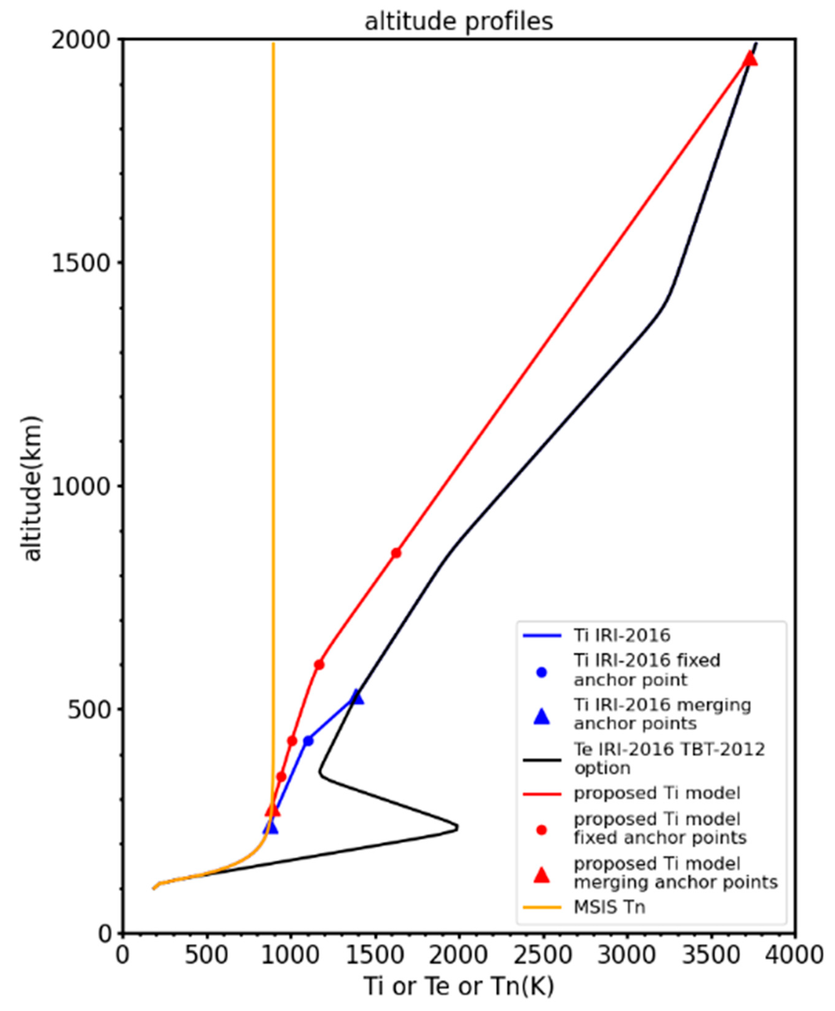
4. Altitude Profiles

Once the global models are established for the four fixed altitudes, as described in the section above, they are combined to produce the full altitude profile in the same way as it is done now in the IRI Ti model. This approach is based on the Booker–Epstein formalism (e.g., [14]), which divides the profile into regions of constant gradient with the boundaries given by anchor altitudes. Epstein-step functions are used to transition from one region to the next thus generating a continuous analytical representation of the Ti gradient and integration then results in the final Ti formula.

To describe the ion temperature height profile above 850 km we adopted the method used in the current IRI ion temperature model [14], i.e., we extrapolate the ion temperature towards higher altitudes using the gradient determined from the section between 600 and 850 km. Next we search for the intersection of this extrapolated Ti profile with the IRI Te profile and then use the intersection height and Ti at that height as an additional anchor point for the Ti profile. We use a similar approach also at the lower altitudes where we can assume thermal equilibrium with the neutrals and therefore Ti = Tn. IRI represents Tn with the help of the NRLMSISE-00 model [16], which is the international standard for Tn. This way we get two more anchor points and hence six anchor altitudes in total (vs. three anchor altitudes in the IRI-2016 Ti model). All these points are then used to construct the entire profile. An example of such a profile is shown in Figure 4.

From this example, we can see that the profile according to the proposed Ti model differs significantly from the profile calculated using the IRI-2016 Ti model. For a large part of the topside, the new Ti model exhibits significantly lower values than the Ti profile according to IRI. The Ti profile from the IRI model merges with the electron temperature profile at an altitude of about 500 km, while the merging height of our new model is close to 2000 km. Note that the data-based Ti values at anchor altitudes of 600 and 850 km are indeed lower than the corresponding model Te values.

5. Model Results and Examples

As an example of the model results, we generated global maps for low and high solar activity. Figure 5 shows these contour plots of the whole Ti model for all four fixed anchor altitudes and for both seasons for conditions of solar minimum (calculated for PF10.7 = 70). Figure 6 shows the same but for solar maximum conditions (calculated for PF10.7 = 200). For both extreme levels of solar activity, it can generally be said that the model confirms the well-known fact that the ion temperature increases with altitude and with latitude and that nighttime temperature values are lower than daytime temperature values, which is particularly evident at the equator and low latitudes, and also that the summer hemisphere is warmer than the winter hemisphere. We also note that these extremely different levels of solar activity (solar maximum vs. solar minimum) cause rather strong changes in the ion temperature. Nighttime Ti at 350 km altitude and at low and mid-latitudes is lower than 800 K at solar minimum, but higher than 1100 K at solar maximum. Daytime ion temperature at solar minimum is also very low about 900 K but at solar maximum reaches 1400 K. This is different from the much smaller changes seen in electron temperature (e.g., [31]). Interestingly, at 850 km altitude in the daytime the relative difference between solar maximum and minimum is much smaller than at lower altitudes (350 and 430 km). Additionally, even in some cases, the proposed model predicts that Ti is higher during solar minima than maxima. This indicates that ion cooling is strongly dominated by neutral particles at low altitudes, while at 850 km the cooling by neutral does not play such a role, but heating of ions by electrons is more dominant. Additionally, interesting is the existence of a morning peak in Ti at equatorial latitudes and its development. The morning peak (so-called morning overshoot) is a distinct feature of the electron temperature (e.g., [37,38]). It is dominant at low altitudes and persists up to 850 km. However, at very high altitudes the peak becomes broader and less apparent because of high daytime Te values over the equator (e.g., see contours in [2]). Due to the strong coupling between electrons and ions, a similar peak can be expected also for Ti as the secondary effect of the heating of ions by thermal electrons. The proposed model shows that the morning peak is mainly present at solar minimum and at an altitude of 600 km (peak maximum about 1700 K). At 850 km the Ti morning peak similarly to the Te peak seems to be less apparent due to increased daytime ion temperature values compared to lower altitudes. At 430 km altitude and below the peak is very weak, and hardly captured by the model. At solar maximum our Ti model shows that the morning peak is present at 600 km but its maximum value (about 1500 K) is slightly lower than at solar minimum and since the nighttime temperature values are high (>1100 K) it appears to be much less prominent then at solar minimum. This again confirms that at high solar activity the expanded neutral atmosphere causes increased ion cooling at altitudes below 850 km.

6. Comparisons with Data

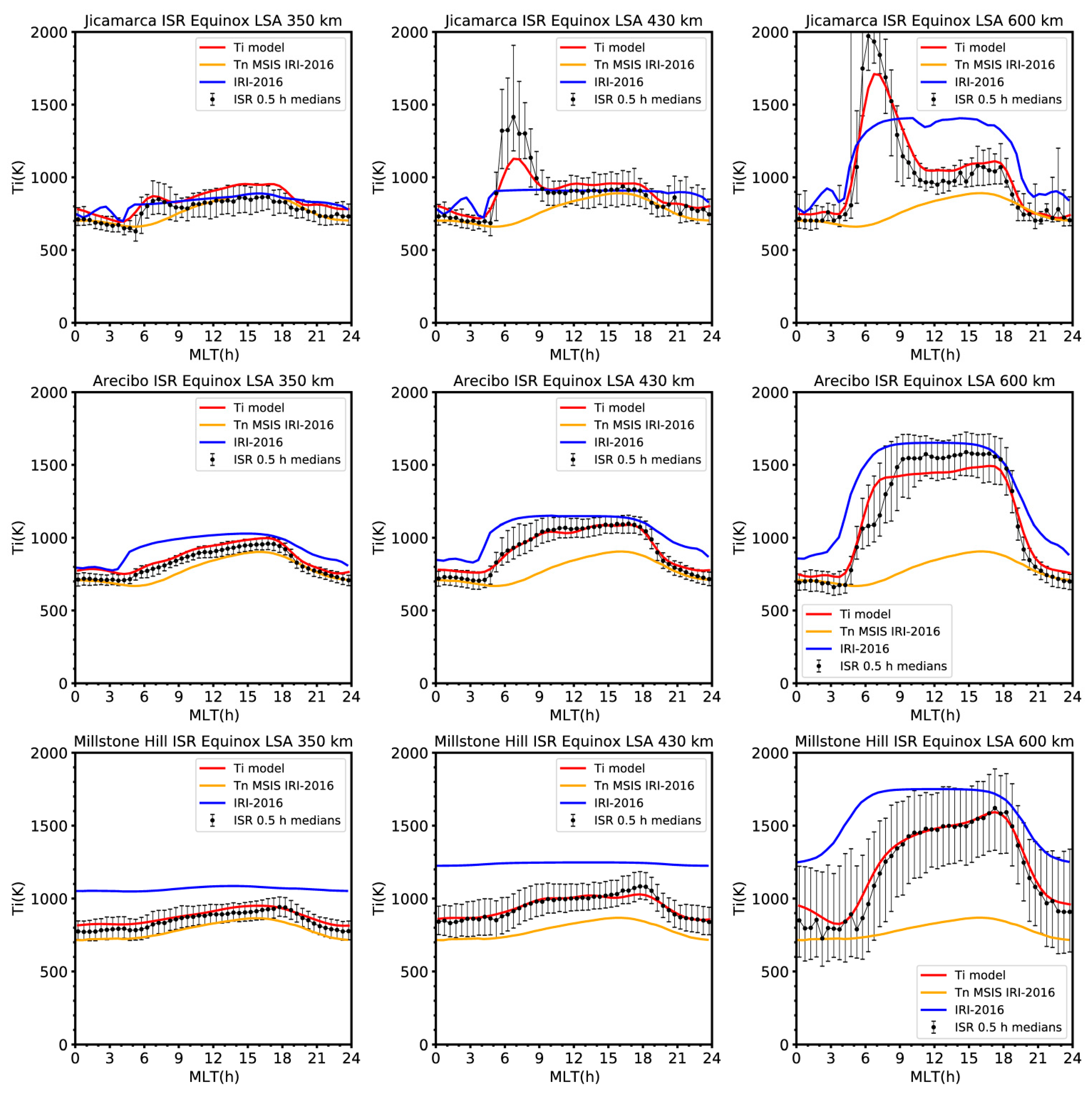
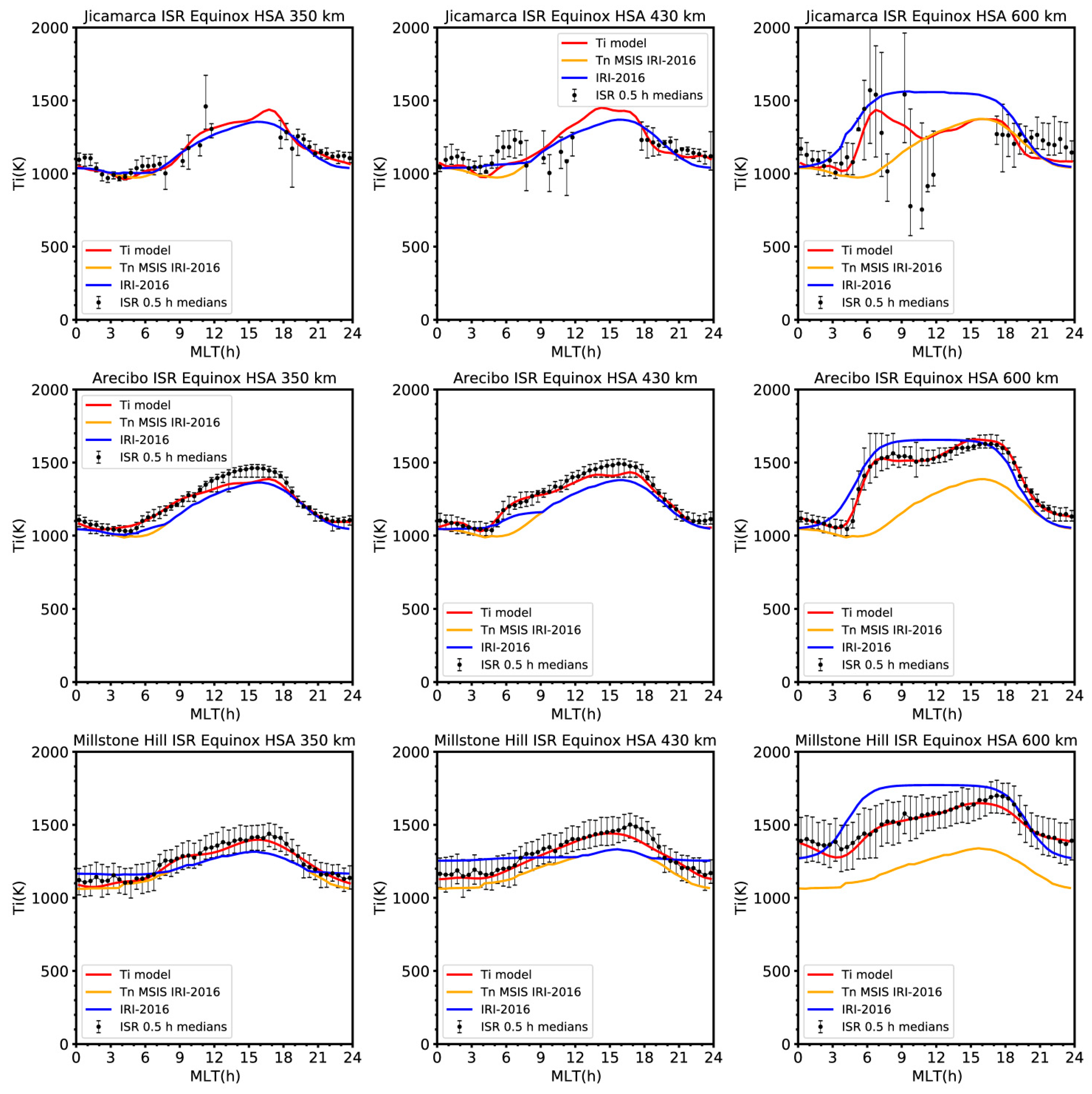
6.1. Comparisons with Jicamarca, Arecibo and Millstone Hill ISR Data

In this section, we present a comparison of the model values with the incoherent scatter radar data. These are the same data that we had used for determining correction terms for the satellite data with which the model was built (see Section 2.1). Since our comparison is limited to model assessment for equinox and high and low solar activity at the anchor altitudes of 350, 430 and 600 km a more detailed comparison will be presented in follow-on paper. Figure 7 shows the comparison of our model and of the current IRI model with Jicamarca, Arecibo, and Millstone Hill ISR data for low solar activity with respect to magnetic local time variation. The ISR data were selected for PF10.7 < 95, from the intervals ±30 days centered on 21 March and 23 September, and three altitudes (350 ± 35 km, 430 ± 43 km, and 600 ± 60 km). The data treatment with respect to measurement uncertainty and possible errors was the same as described in the Section 2.1. We binned this data into 0.5 h of magnetic local time intervals centered at 0.25, 0.5, ..., 23.75 h. In each bin, medians and upper and lower quartiles were evaluated (black circles and error bars). The proposed Ti model is shown by the red line. Each panel corresponds to a specific altitude and ISR; rows distinguish individual ISRs and columns distinguish different altitudes. Due to the large amount of the ISR data values, we run the proposed Ti model for following conditions; the March equinox (for the September equinox the model gives the same result) and PF10.7 = 82.5 (we found that this value was close to the average PF10.7 for the ISR data satisfying PF10.7 < 95). For the IRI-2016 Ti model (shown by the blue line), we searched for such an equinox since 1970 and its close vicinity (±1 day) for which PF10.7 = 82.5 ± 2 s.f.u. because the primary input to the IRI model is the date. To better assess ion temperature variations, we also included Tn values calculated by the IRI code (orange line). Overall, the plots show that the newly proposed Ti model expresses the main features of the diurnal variation of Ti observed by the ISRs. Deviations from the medians are mostly within the variance given by the interquartile range.

For the magnetic equator (Jicamarca-first row) the newly proposed Ti model captures the morning peak quite well, as shown by the ISR data, especially at 600 km altitude contrary to the current IRI model. Evidence that IRI does not include the morning peak was also presented by Coley et al. [39] and Rana et al. [40]. Some underestimation of the peak amplitude by the model, especially at 430 km, can be due to limitations in the model’s temporal resolution. The IRI Ti model shows reasonably good agreement with Jicamarca ISR data at 350 km altitude, but significant differences at 600 km overestimating Ti in the daytime and underestimating it in the morning peak. For all three altitudes IRI predicts a nighttime peak at around 2.5 h MLT that is not observed by the Jicamarca ISR. Ti at the equator is close to Tn at 350 and 430 km altitude, except for the morning increase where heating of ions by hotter electrons plays a role. At an altitude of 600 km, there is also a noticeable difference between Tn and Ti during the day.

At low mid-latitudes (Arecibo-middle row), well away from the equator, the proposed Ti model agrees with the ISR data quite well contrary to the IRI Ti model, that tends to overestimate the ISR data. Interestingly, the morning peak in Ti is no longer observed in the data. The ion temperature can be considered close to Tn at an altitude of 350 km, but above this altitude this is only valid at nighttime.

Going even further away from the equator, at high mid-latitudes (Millstone Hill) an even greater difference between the IRI Ti model and the data is evident, while the newly proposed Ti model expresses the diurnal variation observed by the ISR very well. The IRI Ti model at these latitudes has the worst performance of all three latitude zones. At the two lower altitudes, the IRI ion temperature is almost constant throughout the day and night. Comparison with Tn shows that Ti is significantly higher than Tn even at nighttime.

Figure 8 shows our comparison for high solar activity. The ISR data were selected for 180 < PF10.7 < 220 and thus the proposed Ti model was run for PF10.7 = 200 and IRI was calculated for an equinoctial day that meets this condition. As in the case of low solar activity, the proposed Ti model again agrees with the ISR data quite well. Ti data from the Jicamarca ISR show a surprisingly large scatter especially before noon, and data are completely missing during the afternoon and until sunset. The IRI Ti model at the equator again shows a good agreement at 350 km and 430 km. Different from the low solar activity case the Ti morning peak seems to be absent at 350 and 430 km at high solar activity.

At an altitude of 600 km, the proposed Ti model suggests the presence of a peak with maximum between 6 and 7 h MLT, but it is much less pronounced than at low solar activity and is difficult to identify in the ISR data due to the large data scatter. With the exception of dawn, Ti appears to be strongly coupled with Tn at the geomagnetic equator at all three altitudes.

At Arecibo, the proposed Ti model tends to somewhat underestimate the measurements at the afternoon Ti maximum for both lower altitudes. The IRI Ti model underestimates the ISR observations, contrary to the low solar activity case at the same location (Figure 7). The IRI values appear to be elevated by Tn at daytime because they are constrained by the condition Ti ≥ Tn (blue line overlays the orange line). At 600 km altitude, the Ti observations from the Arecibo ISR exhibit two maxima, which seem to be related to after-dawn and pre-dusk effects, and these are well captured by our Ti model. The IRI Ti model, on the other hand, does not reproduce this variation and shows a flat daytime variation instead. We also note that daytime Ti at Arecibo at high solar activity is significantly higher than Tn, most likely due to the increased heat flux from the plasmasphere.

Finally, our comparison with the Millstone Hill ISR observations shows that the proposed Ti model fits the data exceptionally well, while the IRI-2016 model only does well for the lowest altitude, at 430 km, and 600 km it shows a mixed performance, partially underestimating and partially overestimating the observational data and again, Ti is higher than Tn at an altitude of 430 km and above.

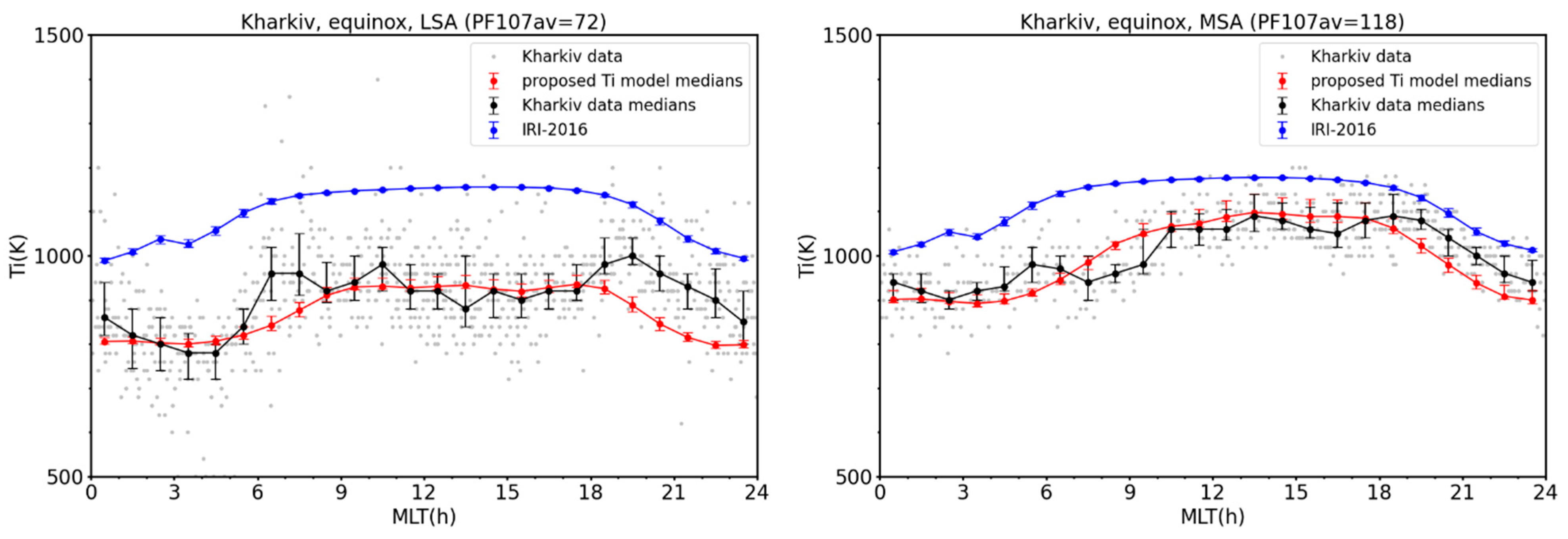
6.2. Comparisons with Kharkiv ISR Ti Data

For comparison with the data that were used neither for model built nor for data correction, we took advantage of Kharkiv ISR measurements. The Kharkiv incoherent scatter radar, its capabilities, and observational results were described by Kotov et al. [41,42,43,44]. The Kharkiv ISR is located in Ukraine near the city of Kharkiv at geographical latitude 49.6° N and geographical longitude 36.3° E, which corresponds to invdip ≈47° and thus represents a region between the Arecibo and Millstone Hill ISRs, which are all in the Americas longitude sector. A limited amount of data covering periods of low and medium solar activity from several recent measurement campaigns was available for this study and is listed in

Table 4. Kharkiv ISR Ti measurements intervals for the equinoxes.

Month	Day Range	Year	$\overline{\mathit{P}\mathit{F}10.7}$
October	28–30	2004	119
September	20–22	2006	75
September	24–27	2007	67
September	23–24	2008	68
September–October	29–01	2009	71
September	20–22	2010	82
September	25–27	2012	128
March	19–21	2013	111
September	24–26	2013	115
March	28–29	2018	69

.

Again, we limited our comparison to the equinoxes. The comparison was made for an altitude of 400 km, which corresponds to the position between the lowest and the second lowest anchor point of the proposed Ti model. Thus, we can also check how good the interpolation in height is using Booker profiles. Figure 9 shows the comparison of the proposed Ti model (red line), IRI-2016 Ti model (blue line) and Kharkiv data (black line, grey dots–individual measurements). In this comparison the model values were calculated exactly for each ISR measurement. Then, we calculated 1 h medians and the upper and lower quartiles, as in the case of the measured data. From both panels we can see that the proposed Ti model fits the data well for most MLTs, while the IRI model overestimates the measurements for all times. We would also like to note that, due to the limited amount of data (Table 4), the plot shown cannot be considered as fully representative of the climatological MLT pattern of Ti. Therefore, we computed the model values for each measurement and then we calculated medians from them. The errors bars determined from calculated values of both models are very small, hardly visible on the plots. This suggests that other dependencies, e.g., seasonal, etc., are not mixed in the data. The overestimation by IRI is consistent with the results of the comparison with the Millstone Hill data for low solar activity (Figure 6, left and middle panels, bottom row).

7. Discussion and Conclusions

In this paper, we present a newly proposed global empirical ion temperature (Ti) model that is an improvement over the option for Ti included in the IRI-2016 model, which is basically unchanged since it was introduced in the IRI-1990 version of the model [14]. The new model is based on data from a large Ti database compiled by the authors from almost all available Ti measurements by satellites from the late 1960s to the present. The advantage of satellite measurements for the construction of the global model lies in the coverage of all latitudes compared to the incoherent scatter radars (ISRs), of which there are only a few worldwide. However, in this study we used data from both. The ISR data helped us to intercalibrate satellite measurements because data from individual satellite missions often show unacceptable differences when compared with data from other satellites for the same conditions, probably due to differences in the design of individual instruments, their electronics, etc. We made this correction by comparing the median of data binned in altitude, latitude, local time, and solar activity for each satellite and ISR. As we used geomagnetic coordinate (invdip) we neglected the influence of longitude, which can be considered a third-order influence parameter, and thus this version of the model neglects longitudinal differences. We have also neglected the effect of geomagnetic activity, whose influence on the ion temperature at least at low and mid-latitudes on a climatological scale can also be considered a third-order effect. Both effects excluded from the space of modelling parameters for the construction of our model might be included in some future version as an additional additive term based on modelling of the corresponding residuals. The proposed corrections for individual satellites, which we used to intercalibrate the data need to be further investigated specifically for case studies that use only part of a specific satellite data set. The obtained correction equations in Table 2 show that the RPA data tend to overestimate Ti relative to the ISR data in most cases. The overestimation is in general moderate, but in some cases can be as high as 30% or more (Figure 2). However, a discussion of the causes is beyond the scope of this study. The analysis of systematic errors in temperature from satellite RPAs has been dealt with by, e.g., Davidson et al. [45] and Klenzing et al. [46]. Our modelling approach is based on spherical harmonics up to 8th order, which provided good agreement with the data both in latitude (invdip) and local time (MLT) and is different from the IRI model, which is based on just one anchor point, while our model uses four anchor points providing a more detailed representation of the altitudinal structure of the ionospheric Ti profile. The height profile is then constructed using the Booker approach as explained in Section 4, whereby Tn is used as a constraint from below and Te as a constraint from above, as employed in the current IRI model. Compared to the current IRI Ti model the new model is able to pick up much more of the altitudinal, latitudinal, and diurnal structure seen in measurements of the ionospheric ion temperature because of the increased number of anchor points and the high order in the spherical harmonics used to describe variations with MLT and invdip. Comparison with the data (Figure 7, Figure 8 and Figure 9) shows a significant improvement over the IRI model, which shows systematic limitations, especially at mid-latitudes towards the poles and at higher altitudes (~600 km). The main results of this paper are as follows:

–

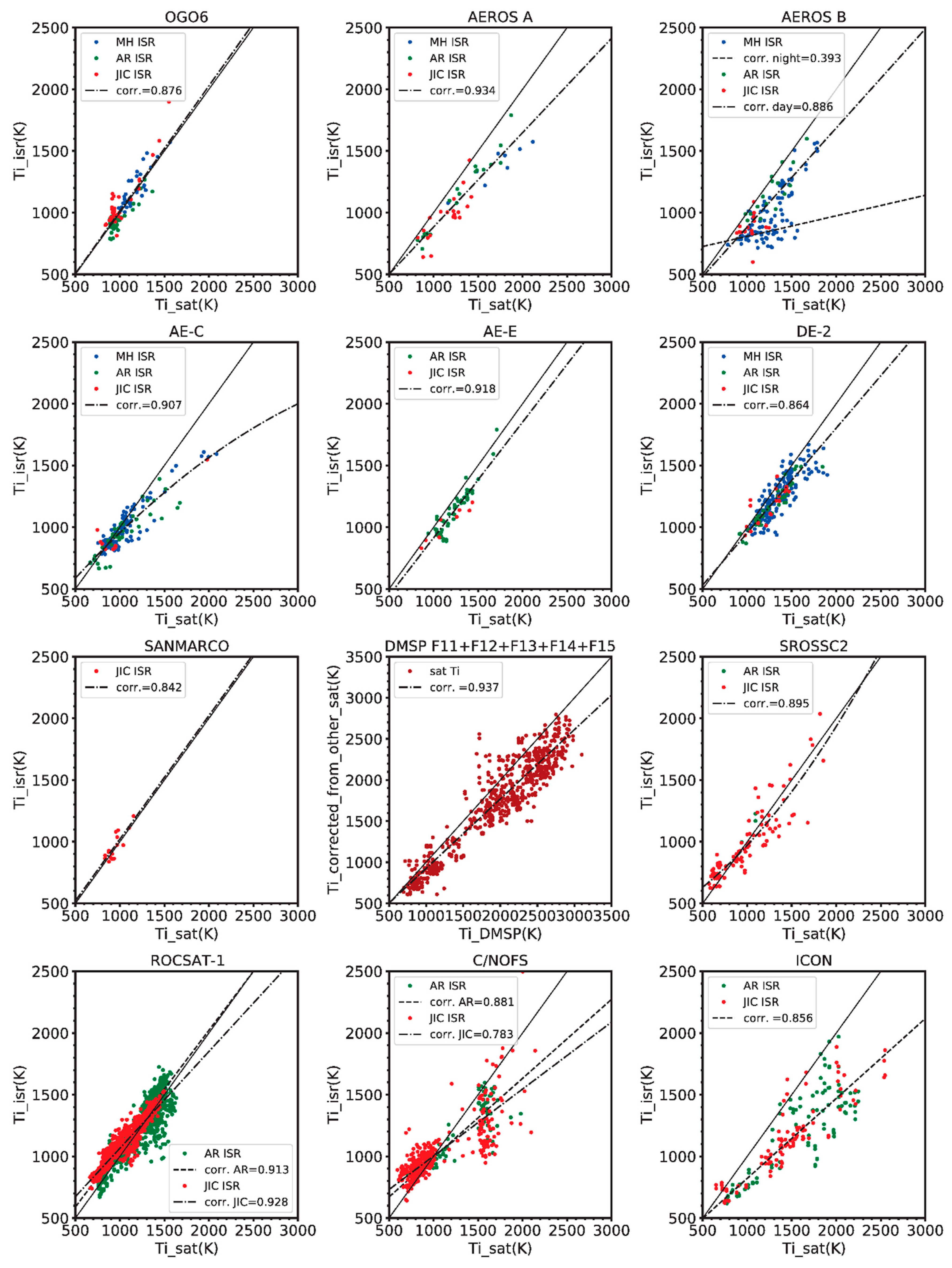
Correction factors were determined for a large number satellite Ti measurements based on comparisons with ISR data.

–

A global ion temperature model was developed based on a database of these corrected satellite Ti measurements.

–

The model represents the climatology of the ion temperature at altitudes from 350 to 850 km using global sub-models at four fixed altitudes.

–

Below an altitude of 350 km, the model uses a connection to Tn and above 850 km a connection to Te.

–

The dependence on solar activity (PF10.7 as a proxy index) is expressed as an additive term that includes both linear and quadratic dependencies.

–

Comparison with ISR data (Jicamarca, Arecibo, Millstone Hill, and Kharkiv) shows that the model describes the diurnal variation quite well for both low and high solar activity at different altitudes and latitudes.

–

Different from the current IRI model the new model captures the morning peak and its dependence on solar activity and altitude, with the peak being most pronounced during periods of low solar activity and at ~600 km altitude.

–

A comparison of the IRI and our new model with the data used in the model developments highlights fundamental flaws of the current IRI Ti model, while the new model is fully consistent with this large data base and is therefore an appropriate alternative to the current model.

–

Future developments could include an extension to include third order dependencies such as magnetic activity or longitude and the use of data from more recent missions (COSMIC-2), and possibly fully integrate ISR data into the model including data from ISRs not yet included like EISCAT, Pokker Flat, etc.

–

The model is available as a subroutine in FORTRAN 77.

References

1. Banks, P.M.; Kockarts, G. Aeronomy; Academic Press: New York, NY, USA, 1973; p. 2. [Google Scholar]
2. Truhlik, V.; Bilitza, D.; Triskova, L. A new global empirical model of the electron temperature with the inclusion of the solar activity variations for IRI. Earth Planets Space 2012, 64, 531–543. [Google Scholar] [CrossRef] [Green Version]
3. Brace, L.H.; Theis, R.F. Global Empirical-Models of Ionospheric Electron-Temperature in the Upper F-Region and Plasmasphere Based on Insitu Measurements from the Atmosphere Explorer-C, Isis-1 and Isis-2 Satellites. J. Atmos. Terr. Phys. 1981, 43, 1317–1343. [Google Scholar] [CrossRef]
4. Bilitza, D.; Brace, L.H.; Theis, R.F. Modelling of ionospheric temperature profiles. Adv. Space Res. 1985, 5, 53–58. [Google Scholar] [CrossRef]
5. Bilitza, D.; Truhlik, V.; Richards, P.; Abe, T.; Triskova, L. Solar cycle variations of mid-latitude electron density and temperature: Satellite measurements and model calculations. Adv. Space Res. 2007, 39, 779–789. [Google Scholar] [CrossRef]
6. Schunk, R.W.; Nagy, A.F. Electron Temperatures in F-Region of Ionosphere—Theory and Observations. Rev. Geophys. 1978, 16, 355–399. [Google Scholar] [CrossRef]
7. Mott-Smith, H.M.; Langmuir, I. The theory of collectors in gaseous discharges. Phys. Rev. 1926, 28, 727. [Google Scholar] [CrossRef]
8. Knudsen, W.C. Evaluation and Demonstration of Use of Retarding Potential Analyzers for Measuring Several Ionospheric Quantities. J. Geophys Res. 1966, 71, 4669–4678. [Google Scholar] [CrossRef]
9. Knudsen, D.; Burchill, J.; Buchert, S.; Eriksson, A.; Gill, R.; Wahlund, J.E.; Åhlén, L.; Smith, M.; Moffat, B. Thermal ion imagers and Langmuir probes in the Swarm electric field instruments. J. Geophys. Res. Space Phys. 2017, 122, 2655–2673. [Google Scholar] [CrossRef]
10. Bilitza, D. Electron and ion temperature data for ionospheric modelling. Adv. Space Res. 1991, 11, 139–148. [Google Scholar] [CrossRef]
11. Schunk, R.W.; Nagy, A.F. Ionospheres of the Terrestrial Planets. Rev. Geophys. 1980, 18, 813–852. [Google Scholar] [CrossRef]
12. Hsu, C.T.; Heelis, R.A. Measurement of Individual H+ and O+ Ion Temperatures in the Topside Ionosphere. J. Geophys. Res. Space Phys. 2018, 123, 1525–1533. [Google Scholar] [CrossRef]
13. Bilitza, D.; Altadill, D.; Truhlik, V.; Shubin, V.; Galkin, I.; Reinisch, B.; Huang, X. International Reference Ionosphere 2016: From ionospheric climate to real-time weather predictions. Space Weather 2017, 15, 418–429. [Google Scholar] [CrossRef]
14. Bilitza, D. International Reference Ionosphere 1990; Report 90-22; National Space Science Data Center: Greenbelt, MD, USA, 1990.
15. Pignalberi, A.; Aksonova, K.D.; Zhang, S.-R.; Truhlik, V.; Gurram, P.; Pavlou, C. Climatological study of the ion temperature in the ionosphere as recorded by Millstone Hill incoherent scatter radar and comparison with the IRI model. Adv. Space Res. 2021, 68, 2186–2203. [Google Scholar] [CrossRef]
16. Picone, J.M.; Hedin, A.E.; Drob, D.P.; Aikin, A.C. NRLMSISE-00 empirical model of the atmosphere: Statistical comparisons and scientific issues. J. Geophys. Res. Space Phys. 2002, 107, 1468–1483. [Google Scholar] [CrossRef]
17. Heelis, R.; Hanson, W. Measurements of thermal ion drift velocity and temperature using planar sensors. Geophys. Monogr. Am. Geophys. Union 1998, 102, 61–72. [Google Scholar]
18. Hanson, W.B.; Sanatani, S.; Zuccaro, D.; Flowerday, T.W. Plasma Measurements with Retarding Potential Analyzer on Ogo-6. J. Geophys. Res. 1970, 75, 5483–5501. [Google Scholar] [CrossRef]
19. Spenner, K.; Dumbs, A. Retarding Potential Analyzer on Aeros-B. Z. Geophys. 1974, 40, 585–592. [Google Scholar]
20. Hanson, W.B.; Zuccaro, D.R.; Lippincott, C.R.; Sanatani, S. Retarding-Potential Analyzer on Atmosphere Explorer. Radio Sci. 1973, 8, 333–339. [Google Scholar] [CrossRef]
21. Hanson, W.; Heelis, R.; Power, R.; Lippincott, C.; Zuccaro, D.; Holt, B.; Harmon, L.; Sanatani, S. The retarding potential analyzer for Dynamics Explorer-B. Space Sci. Instrum. 1981, 5, 503–510. [Google Scholar]
22. Broglio, L.; Ponzi, U.; Arduini, C. The San Marco 5 mission. Adv. Space Res. 1993, 13, 165–184. [Google Scholar] [CrossRef]
23. Afonin, V.V.; Smirnova, N.F. Optimization of Complex Experiment on Measurement of the Cold Plasma Parameters; Space Research Institute: Moscow, Russia, 1990; pp. 1–21. [Google Scholar]
24. Rich, F. Users Guide for the Topside Ionospheric Plasma Monitor (SSIES, SSIES-2 and SSIES-3) on Spacecraft of the Defense Meteorological Satellite Program., Volume 1: Technical Description; PHILLIPS LABORATORY, Hanscom Air Force Base: Bedford, MA, USA, 1994. [Google Scholar]
25. Garg, S.; Anand, J.; Bahl, M.; Subrahmanyam, P.; Rajput, S.; Maini, H.; Chopra, P.; John, T.; Singhal, S.; Singh, V.; et al. RPA Aeronomy Experiment Onboard the Indian Satellite SROSS-C2—Some Important Aspects of the Payload and Satellite. Indian J. Radio Space Phys. 2003, 32, 5–15. [Google Scholar]
26. Borgohain, A.; Bhuyan, P.K. Solar cycle variation of ion densities measured by SROSS C2 and FORMOSAT-1 over Indian low and equatorial latitudes. J. Geophys. Res. Space Phys. 2010, 115, 1–13. [Google Scholar] [CrossRef] [Green Version]
27. Su, S.-Y.; Yeh, H.C.; Heelis, R.A.; Wu, J.-M.; Yang, S.C.; Lee, L.-F.; Chen, H.L. The ROCSAT-1 IPEI preliminary results: Low-latitude ionospheric plasma and flow variations. Terr. Atmos. Ocean Sci. 1999, 10, 787–804. [Google Scholar] [CrossRef]
28. Chao, C.K.; Su, S.Y.; Yeh, H.C. Ion temperature variation observed by ROCSAT-1 satellite in the afternoon sector and its comparison with IRI-2001 model. Adv. Space Res. 2006, 37, 879–884. [Google Scholar] [CrossRef]
29. de La Beaujardière, O. C/NOFS: A mission to forecast scintillations. J. Atmos. Sol. Terr. Phys. 2004, 66, 1573–1591. [Google Scholar] [CrossRef]
30. Heelis, R.A.; Stoneback, R.A.; Perdue, M.D.; Depew, M.D.; Morgan, W.A.; Mankey, M.W.; Lippincott, C.R.; Harmon, L.L.; Holt, B.J. Ion Velocity Measurements for the Ionospheric Connections Explorer. Space Sci. Rev. 2017, 212, 615–629. [Google Scholar] [CrossRef]
31. Truhlik, V.; Bilitza, D.; Triskova, L. Latitudinal variation of the topside electron temperature at different levels of solar activity. Adv. Space Res. 2009, 44, 693–700. [Google Scholar] [CrossRef]
32. Richards, P.G.; Fennelly, J.A.; Torr, D.G. Euvac—A Solar Euv Flux Model for Aeronomic Calculations. J. Geophys. Res. Space Phys. 1994, 99, 8981–8992. [Google Scholar] [CrossRef]
33. Truhlik, V.; Triskova, L.; Smilauer, J.; Afonin, V.V. Global empirical model of electron temperature in the outer ionosphere for period of high solar activity based on data of three intercosmos satellites. Adv. Space Res. Ser. 2000, 25, 163–169. [Google Scholar] [CrossRef]
34. Truhlik, V.; Triskova, L.; Saxonbergova-Jankovicova, D. Observations of the ion temperature in morning hours in the equatorial topside ionosphere from ICON and other satellites. In Proceedings of the AGU Fall Meeting, San Francisco, CA, USA, 1–17 December 2020; Available online: https://agu2020fallmeeting-agu.ipostersessions.com/Default.aspx?s=D7-4D-E6-A7-05-7A-3B-09-20-07-14-FC-3E-D4-09-D4 (accessed on 7 December 2020).
35. Martinec, Z. Program to Calculate the Least-Squares Estimates of the Spherical Harmonic Expansion Coefficients of an Equally Angular-Gridded Scalar Field. Comput. Phys. Commun. 1991, 64, 140–148. [Google Scholar] [CrossRef]
36. Press, W.H.; Teukolsky, S.A.; Vetterling, W.T.; Flannery, B.P. Numerical Recipes in C: The Art of Scientific Computing, 2nd ed.; Cambridge University Press: New York, NY, USA, 1992. [Google Scholar]
37. Oyama, K.I.; Watanabe, S.; Su, Y.; Takahashi, T.; Hirao, K. Season, local time, and longitude variations of electron temperature at the height of similar to 600 km in the low latitude region. Adv. Space Res. 1996, 18, 269–278. [Google Scholar] [CrossRef]
38. Stolle, C.; Liu, H.; Truhlik, V.; Luhr, H.; Richards, P.G. Solar flux variation of the electron temperature morning overshoot in the equatorial F region. J. Geophys. Res. Space Phys. 2011, 116, 1–13. [Google Scholar] [CrossRef] [Green Version]
39. Coley, W.R.; Heelis, R.A.; Hairston, M.R.; Earle, G.D.; Perdue, M.D.; Power, R.A.; Harmon, L.L.; Holt, B.J.; Lippincott, C.R. Ion temperature and density relationships measured by CINDI from the C/NOFS spacecraft during solar minimum. J. Geophys. Res. Space Phys. 2010, 115, 1–6. [Google Scholar] [CrossRef] [Green Version]
40. Rana, G.; Bardhan, A.; Sharma, D.K.; Yadav, M.K.; Aggarwal, M.; Dudeja, J. Variations of ion density and temperature as measured by ROCSAT-1satellite over the Indian region and comparison with IRI-2016 model. Ann. Geophys. 2019, 62, 11. [Google Scholar] [CrossRef]
41. Kotov, D.V.; Richards, P.G.; Bogomaz, O.V.; Chernogor, L.F.; Truhlik, V.; Emelyanov, L.Y.; Chepurnyy, Y.M.; Domnin, I.F. The importance of neutral hydrogen for the maintenance of the midlatitude winter nighttime ionosphere: Evidence from IS observations at Kharkiv, Ukraine, and field line interhemispheric plasma model simulations. J. Geophys. Res. Space Phys. 2016, 121, 7013–7025. [Google Scholar] [CrossRef] [Green Version]
42. Kotov, D.V.; Richards, P.G.; Truhlik, V.; Bogomaz, O.V.; Shulha, M.O.; Maruyama, N.; Hairston, M.; Miyoshi, Y.; Kasahara, Y.; Kumamoto, A.; et al. Coincident Observations by the Kharkiv IS Radar and Ionosonde, DMSP and Arase (ERG) Satellites, and FLIP Model Simulations: Implications for the NRLMSISE-00 Hydrogen Density, Plasmasphere, and Ionosphere. Geophys. Res. Lett 2018, 45, 8062–8071. [Google Scholar] [CrossRef]
43. Kotov, D.V.; Richards, P.G.; Truhlik, V.; Maruyama, N.; Fedrizzi, M.; Shulha, M.O.; Bogomaz, O.V.; Lichtenberger, J.; Hernandez-Pajares, M.; Chernogor, L.F.; et al. Weak Magnetic Storms Can Modulate Ionosphere-Plasmasphere Interaction Significantly: Mechanisms and Manifestations at Mid-Latitudes. J. Geophys. Res. Space Phys. 2019, 124, 9665–9675. [Google Scholar] [CrossRef]
44. Kotov, D.V.; Truhlik, V.; Richards, P.G.; Stankov, S.; Bogomaz, O.V.; Chernogor, L.F.; Domnin, I.F. Night-time light ion transition height behaviour over the Kharkiv (50 degrees N, 36 degrees E) IS radar during the equinoxes of 2006–2010. J. Atmos. Sol. Terr. Phys. 2015, 132, 1–12. [Google Scholar] [CrossRef]
45. Davidson, R.; Earle, G.; Klenzing, J.; Heelis, R. A numerical study of geometry dependent errors in velocity, temperature, and density measurements from single grid planar retarding potential analyzers. Phys. Plasmas 2010, 17, 082901. [Google Scholar] [CrossRef]
46. Klenzing, J.; Earle, G.; Heelis, R.; Coley, W. A statistical analysis of systematic errors in temperature and ram velocity estimates from satellite-borne retarding potential analyzers. Phys. Plasmas 2009, 16, 052901. [Google Scholar] [CrossRef]
Figure 1. Year–altitude coverage of data in the database for individual satellite missions and corresponding 81-day running mean of the F10.7 index.
Atmosphere 12 01081 g001
Figure 2. Scatterplots of binned Ti values from ISRs vs. binned Ti values from satellites. The bins corresponding to Jicamarca are shown by red points, Arecibo by green points, and Millstone Hill by blue points. Information on the Pearson correlation coefficient (corr.) is also included. For DMSP (brown points), the scatterplot represents a comparison with already corrected satellite data (vertical axis; “other_sat” stand for DE-2, OGO-6, and C/NOFS). Additionally, shown are the least-square fits to the data (dash-dotted and dashed line) and the line marking perfect agreement: Ti_sat = Ti_isr (solid line).
Atmosphere 12 01081 g002
Figure 3. Histogram (number of data points in 5 km bins vs. altitude) of the ion temperature data in our database.
Atmosphere 12 01081 g003
Figure 4. Example of altitude profiles (case for 21 March 2016; PF10.7 = 92; Solar local time 12 h, geographical latitude = 20°; geographical longitude = 0°) from the proposed Ti model (red line; 4 red circles represent 4 fixed anchor points with altitudes of 350, 430, 600 and 850 km; 2 red triangles symbolize additional anchor points with variable altitudes-lower one a tangent point on the Tn profile (orange line) and higher one an intersection with the Te profile (black line). The corresponding Ti profile computed from the IRI-2016 model is shown in the blue color (one fixed anchor point at 430 km height-circle; two anchor points for the connection with Tn and Te-triangles).
Atmosphere 12 01081 g004
Figure 5. Contour plots of the Ti model for equinox and solstice for the four anchor altitudes during solar minimum (PF10.7 = 70).
Atmosphere 12 01081 g005
Figure 6. Contour plots of the Ti model for equinox and solstice for four altitude intervals and solar maximum (PF10.7 = 200).
Atmosphere 12 01081 g006
Figure 7. Local time variation of Ti for low solar activity (PF10.7 = 82.5) from the three ISRs (black circles—medians, error bars—upper/lower quartile; Jicamarca—upper row, Arecibo—middle row, Millstone Hill—lower row) and for three altitudes (350 km—left column, 430 km—middle column, 600 km—right column). Included is the proposed Ti model (red line), the IRI-2016 Ti model (blue line), and Tn from the IRI-2016/NRLMSISE-00 model (orange line).
Atmosphere 12 01081 g007
Figure 8. The same as Figure 7, but for high solar activity (PF10.7 = 200).
Atmosphere 12 01081 g008
Figure 9. Local time variation of Kharkiv Ti data (grey points—individual measurements; black circles—medians in 1 h wide MLT bins; error bars represent upper and lower quartiles), corresponding medians and lower/upper quartiles from the proposed Ti and IRI-2016 models (red and blue, respectively). The left panel represents low solar activity (LSA) and the right panel represents medium solar activity (MSA).
Atmosphere 12 01081 g009