
Assimilation of Leaf Area Index and Soil Water Index from Satellite Observations in a Land Surface Model in Hungary


Hungarian Meteorological Service, 1024 Budapest, Hungary
*
Author to whom correspondence should be addressed.
Atmosphere 2021, 12(8), 944; https://0-doi-org.brum.beds.ac.uk/10.3390/atmos12080944
Submission received: 6 July 2021
/
Accepted: 20 July 2021
/
Published: 23 July 2021
(This article belongs to the Special Issue Climate Extremes in the Pannonian Basin: Current Approaches and Challenges)
Abstract
:In this study, a Land Data Assimilation System (LDAS) is applied over the Carpathian Basin at the Hungarian Meteorological Service to monitor the above-ground biomass, surface fluxes (carbon and water), and the associated root-zone soil moisture at the regional scale (spatial resolution of 8 km × 8 km) in quasi-real-time. In this system the SURFEX model is used, which applies the vegetation growth version of the Interactions between Soil, Biosphere and Atmosphere (ISBA-A-gs) photosynthesis scheme to describe the evolution of vegetation. SURFEX is forced using the outputs of the ALADIN numerical weather prediction model run operationally at the Hungarian Meteorological Service. First, SURFEX is run in an open-loop (i.e., no assimilation) mode for the period 2008–2015. Secondly, the Extended Kalman Filter (EKF) method is used to assimilate Leaf Area Index (LAI) Spot/Vegetation (until May 2014) and PROBA-V (from June 2014) and Soil Water Index (SWI) ASCAT/Metop satellite measurements. The benefit of LDAS is proved over the whole country and to a selected site in West Hungary (Hegyhátsál). It is demonstrated that the EKF can provide useful information both in wet and dry seasons as well. It is shown that the data assimilation is efficient to describe the inter-annual variability of biomass and soil moisture values. The vegetation development and the water and carbon fluxes vary from season to season and LDAS is a capable tool to monitor the variability of these parameters.
1. Introduction
The accurate description of surface processes is important in several temporal and spatial scales from the weather forecasts to climate change projections as they provide lower boundary conditions for the atmospheric models. Sub-grid scale interactions between the atmosphere and the land surface, as well as soil processes, are described with parametrization in numerical weather prediction (NWP) and climate models. Besides the increasingly sophisticated schemes, in state-of-the-art NWP models, the surface processes of the vegetation, carbon and water cycles are often represented in land surface models (LSM) coupled with the atmospheric model component. Using the atmospheric forcings, LSMs describe the biophysical conditions of the soil, e.g., soil moisture and temperature and the biomass consistently with ecosystem dynamics [1].
LSM forecasts can be improved by involving observations using data assimilation (DA) techniques in which observations are combined with the short-term forecasts in a statistically optimal way. Several DA methods have been developed to estimate the soil parameters. In the early years, when measurements for soil parameters were available only sporadically and with low spatial coverage, the employed techniques were based on atmospheric or screen level analysis resulting from atmospheric data assimilation. For instance, in the lack of screen level analysis in the 90 s, a simple nudging approach was applied at ECMWF to correct the soil moisture using specific humidity analysis at the lowest model level [2]. Later, optimal interpolation (OI) was widely implemented, taking the advantage that the soil moisture analysis relies on the link between the screen-level parameters and the soil moisture [3,4]. An extended Kalman Filter (EKF) allows assimilation of both conventional (screen-level) and non-conventional (satellite) observations to provide surface analysis. Furthermore, to exploit the advantage of the satellite data, EKF, 2D-Var [5], and Ensemble Kalman Filter [6] methods were investigated to generate soil moisture analysis.
Since few in-situ measurements are available and they are not representative, it is important to know how to assimilate satellite data. Several studies have discussed the possibility of the assimilation of remote sensing observations into LSMs [7,8,9,10,11,12,13] and in NWP models [14,15,16,17]. Combining Earth observations (EOs) and LSMs through land data assimilation systems (LDAS) can improve the initial land surface conditions, this can benefit the weather forecasts, including temperature and precipitation predictions [18,19,20]. Various articles have assessed different versions of EKF to assimilate either satellite measurements for soil moisture [10,11,12], LAI [13], or both [1,2,3,4,5,6,7], in LSMs; [11] demonstrated useful increments generated from AMSR-E (Advanced Microwave Scanning Radiometer) soil moisture remote sense observations in the total soil layer. Besides, EKF and the simplified version of EKF were compared, in which the background errors were kept constant. Despite the fact that they produced similar soil analyses, EKF was recommended for future work. It was also presented that it is necessary to remove the seasonal bias between the satellite observation and the model soil moisture by using a Cumulative Distribution Function (CDF) matching technique.
The SURFace EXternalisée (SURFEX) LSM model applies Interaction between Soil, Biosphere, and Atmosphere (ISBA), a scheme which simulates these processes [21]. It is an externalised surface model capable of being coupled to any atmospheric numerical weather prediction (NWP) model.
The benefit of joint assimilation of SSM and LAI by using the multi-patch, multi-layer diffusion version of SURFEX ISBA model (LDAS-Monde), was pointed out in [9,22]. The evolution of the above-ground biomass changes in a lagged response to the modified soil moisture conditions. The model sensitivity to the observed SSM decreases from the top to the deep layers and there was almost no impact from 60 cm downwards, and the assimilation is more efficient in summer and autumn than in winter and spring. It was shown that the assimilation worked effectively, but the impact of the assimilation on the vegetation phenology and the water and carbon fluxes varied from season to season. Besides, the global LDAS-Monde model can detect, monitor, and forecast extreme weather, such as drought, or heat-wave events, which were performed by computing anomalies.
A wide range of satellite-based biophysical products are provided by the Copernicus Land Service, which had been built in the framework of the FP7 Geoland2 project (http://www.gmes-geoland.info, accessed on 21 July 2021). The developments were continued in the ImagineS (Implementation of Multi-scale AGricultural INdicators Exploiting Sentinels) project to support the operations of the global component of the Copernicus Land service, preparing for the use of the Sentinel data in an operational context (http://fp7-imagines.eu/, accessed on 21 July 2021). Both projects aimed to organise a qualified production network, to set up user-driven biophysical products describing the vegetation and the energy and water budgets. Within the framework of these projects, several studies demonstrated the added values of regional or global LDAS, to monitor crop/fodder production together with carbon and water fluxes [7,9]. The aim of the Hungarian Meteorological Service in both projects was to adopt, develop and validate the regional LDAS and quasi-real-time modeling of biomass, soil moisture, natural carbon dioxide, and water vapor fluxes for the territory of Hungary, using satellite measurements.
Vegetation monitoring is an important task in Hungary. As the inter-annual variability of the vegetation is quite high in Hungary (considering its dry continental climate), and since the proportion of irrigated areas is rather small (1–2%, https://data.worldbank.org/indicator/AG.LND.IRIG.AG.ZS?locations=HU, accessed on 21 July 2021), the drought exposure of agriculture is very high. In addition, agriculture accounts for a significant share of the national economy. Therefore, it is important to estimate the evolution of the vegetation using numerical methods (e.g., LDAS). The main objective of this study is to assess the performance of the system established in Geoland2 and ImagineS projects over the Carpathian Basin, i.e., how SURFEX can provide the above-ground biomass, soil moisture, water and carbon fluxes, and how LDAS captures the benefits of the assimilation of the remote sensing observations and improves the biomass as well as the soil moisture response under different climatic conditions. In this paper, evaluations of the model runs against satellite data, and in-situ measurements are shown. The paper is structured in the following way. In Section 2 the SURFEX model and the ISBA-A-gs scheme are introduced, and then the applied data and assimilation methods are described. The seasonal-based CDF technique is also explained. In Section 3, the results are presented: the impact of assimilation and the seasonal cycle of LAI, soil moisture, carbon and water fluxes, the inter-annual variability of LAI and soil moisture through the drought monitoring. Finally, the main conclusions and outlooks are summarised in Section 4.
2. Materials and Methods
2.1. SURFEX Model and ISBA-A-gs Scheme
In the SURFEX system, each surface grid point is separated into 4 different tiles: nature, sea, lake, and town. The model handles each tile independently. In our work, only the nature tile was treated, and was further divided into 12 patches according to the vegetation or surface type: bare soil, rock, permanent snow, deciduous tree, coniferous trees, broadleaf evergreen tree, C3 crops, C4 crops, irrigated crops, grassland, tropical grassland, parks, and gardens. The model solves the prognostic equations for soil moisture and temperature and calculates the surface fluxes separately for the different patches. Each patch uses the same atmospheric forcing (air temperature, humidity, wind speed, downward long- and shortwave radiation, pressure, precipitation), but the parameter settings are different and independent of each other. The resulting surface fluxes (momentum, sensible- and latent heat) are averaged according to the area fraction of the patches and returned to the atmosphere. Surface parameters are defined by physiographic databases: GTOPO30 for orography, ECOCLIMAP-II for surface covers [23], and FAO for soil texture. The dominant ecosystems in our domain are C3 crops (27%), grassland (21%), deciduous trees (19%), C4 crops (15%), bare soil (8%), and a coniferous tree (6%).
The nature tile is simulated with the ISBA scheme [24,25], which computes the exchanges of energy and water between the continuum soil–vegetation–snow and the atmosphere above. In ISBA, a 3-layer soil scheme is used (surface 0–1 cm, root zone 0–2 m, and deep soil 2–3 m). The soil prognostic variables (temperature, water content, and intercepted water content) are calculated using the force–restore method [25]. The force terms for temperature are radiation, latent and sensible heat flux. The restore term relaxes the temperature to the mean soil temperature. The force terms for soil water content are precipitation and evaporation. The restoring term describes how the system reaches equilibrium.
A more recent version of the model named ISBA-A-gs [26,27,28,29] accounts for a simplified photosynthesis model where the evaporation is controlled by the aperture of the stomata and this mechanism regulates the balance between the transpiration and the assimilation of CO2. The model is suitable for describing the evolution of the vegetation because biomass is a prognostic variable. The growing of vegetation is due to photosynthesis (CO2 assimilation) while its decrease is due to soil moisture stress or senescence. The model considers the soil moisture stress in photosynthesis [28]. Plants can have two strategies to the stress: a drought avoiding and a drought tolerant strategy. The growth of the biomass is proportional to the daily net assimilated CO2, while the decrease is described by an exponential function.
One of the carbon-fluxes, GPP (Gross Primary Production), is the assimilated CO2 by the plants. Photosynthesis is first calculated at the leaf scale. The sensitivity of the plant to the specific humidity of the air is also included in the calculations. The net assimilation is integrated over the canopy, and GPP is calculated as the sum of the total assimilation and the dark respiration. NEE is the net CO2 flux of the ecosystem.
2.2. Data
To improve the accuracy of the initial fields, data assimilation is used. The analyzed variables are the Leaf Area Index (LAI) and the root-zone soil moisture (WG2). These variables have a long memory (slow variability in time), and furthermore LAI and soil moisture influence to a great extent the evolution of photosynthesis, and through this, the value of carbon fluxes.
2.2.1. Atmospheric Forcing Data
SURFEX was run in offline mode, this means that the surface fluxes have no effect on the atmospheric fields, but the model needs meteorological data (air temperature, humidity, wind speed, precipitation, long- and short-wave radiation). This information was obtained from the ALADIN (Aire Limitée Adaptation dynamique Développement InterNational) numerical weather prediction model [30], except for the radiation, which is derived from LandSAF (Land Surface Analysis Satellite Applications Facility) observation. The reason for this choice is that radiation influences to a great extent the photosynthesis and the output fields of NWP are not as accurate as of the satellite observations. ALADIN is a numerical weather prediction model used operationally at HMS to produce daily weather forecasts [31]. It is a hydrostatic, spectral limited area model which describes the time evolution of the processes in the atmosphere. The model has its data assimilation system: incremental 3D-Var and an OI technique for the upper-air and surface analysis respectively [32]. The model is applied for a domain over Europe with 8 km x 8 km horizontal resolution and 49 vertical layers. The lateral boundary conditions are provided by ECMWF/IFS model at 3-hourly time intervals.
The forcing dataset covered the period 2007–2015 and included meteorological information at 3-hourly time intervals.
2.2.2. GEOV1 Leaf Area Index
Satellite observations for LAI are derived from SPOT-VGT (until May 2014) and PROBA-V (from June 2014) satellite data produced by European Copernicus Global Land Service (https://land.copernicus.eu/global/, accessed on 21 July 2021). The SPOT/VGT LAI Version 1 (GEOV1) is derived from the SPOT/VGT Top of Atmosphere (TOA) reflectances provided by the SPOT/VEGETATION program [33], while the PROBA-V LAI Version 1 is derived from the SPOT/VGT-like Top of Atmosphere (TOA) PROBA-V reflectances generated by the PROBA2VGT module. This module ensures the consistency of the time series when moving from SPOT/VGT to PROBA-V data. Both products are provided at a spatial resolution of 1 km and 10 days sampling time in a regular latitude/longitude grid. The accuracy (RMSE) of GEOV1 products compared to the reference in-situ data set is 0.7 for LAI [34].
2.2.3. ASCAT Soil Water Index
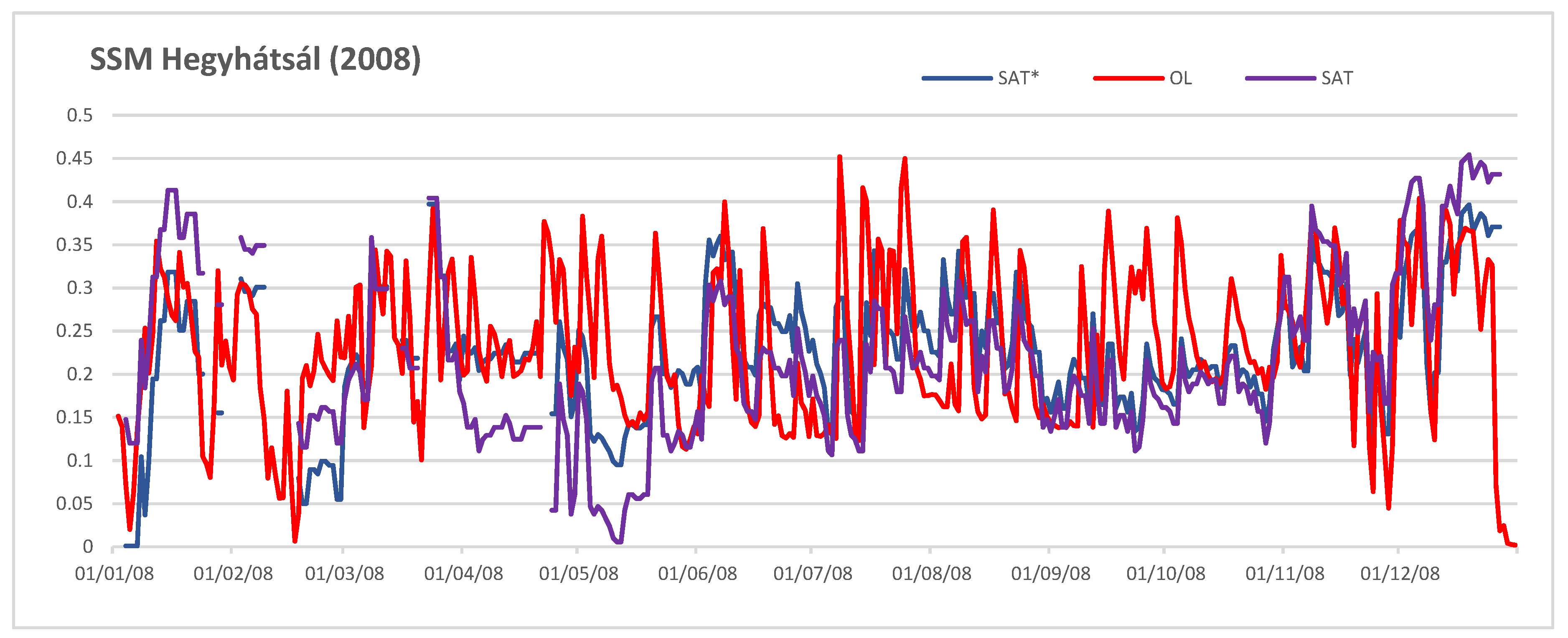
For analyzing the root-zone soil moisture, the surface soil moisture (SSM) needs to be assimilated, which is derived from an SWI (Soil Water Index) product. SWI is calculated from MetOp. ASCAT observations using a recursive exponential filter [35]. SWI is obtained at 0.1 degree spatial resolution with daily sampling [36]. To get an SSM value from SWI information, the following relation is used: SSM = SWI × (wmax − wmin) + wmin, where wmin and wmax are the minimal and maximal SSM values that the model can produce at a given grid point during the 2008–2015 period. Since the soil moisture quantity observed by remote sensors differs from that defined in models, soil moisture data must be rescaled before assimilation, to be consistent with the model climatology [37]. The ASCAT data are bias-corrected concerning the model climatology by using a seasonal-based CDF (Cumulative Distribution Function) matching technique, as described in [37]. Figure 2 compares the open-loop model simulation with the raw ASCAT and the CDF rescaled ASCAT time series at Hegyhátsál (located in the western part of Hungary). The CDF matching with seasonal correction improves the temporal correlations between the data and the model.
2.2.4. FLUXNET Site, Hegyhátsál
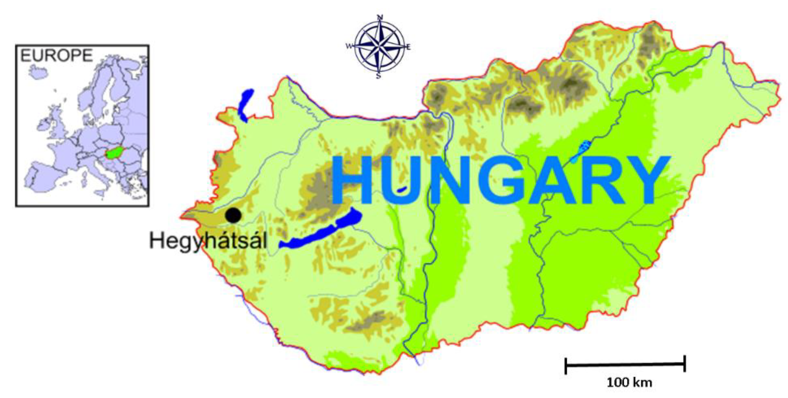
FLUXNET is a global network of micrometeorological tower sites that measure the exchanges of carbon dioxide, water vapor, and energy between terrestrial ecosystems and the atmosphere using eddy covariance methods [38]. Hegyhátsál is a FLUXNET site [39] located in the flat region of western Hungary (Figure 3), surrounded by semi-natural grass fields (hay meadows), agricultural fields (mostly crops), and forest patches. The soil type of the region is brown forest soil.
For the long-term monitoring of the surface-atmosphere exchange of nitrous oxide in the region, an eddy covariance system was added to the instrumentation of the Hegyhátsál tall tower greenhouse gas monitoring station. The eddy covariance system is operated at 82 m and 3 m height [40,41,42]. In addition to the daily continuous carbon dioxide and water vapor exchange measurements, weekly LAI and daily soil moisture (derived from 10–30 cm depth) observations are also conducted.
2.3. Data Assimilation
Extended Kalman Filter (EKF) assimilation method was performed to analyse LAI superficial and root-zone water contents [14,43,44]. To determine these values, observations, and background (model forecast starting from a previous cycle) information need to be considered. In EKF, dynamically changing coefficients are used, and the analysis is obtained:
where x is the model state vector (a means analysis, f means forecast), y is the observation vector, H is the non-linear observation operator, K is the Kalman gain matrix:
K = BHT ( HBHT + R )−1,
The K gain matrix represents the relative importance of the error of the observation concerning the prior estimate. H is the linearised observation operator, B and R are the covariance matrices of the background errors and the observation errors, respectively. They are assumed to be diagonal, and R is time-invariant. In the simplified version of the EKF, namely SEKF, the background covariance matrix B does not evolve with time. In some previous studies [7,8,45], diagonal background error covariance was used at the start of each cycle, but the implicit background covariances are derived from H matrix at the analysis time.
The analysis equation is solved at each grid point independently, as we assume there is no correlation between neighbouring grid points. On the other hand, one grid point is divided into 12 patches, but the observations contain only information from the average value of the grid. Hence in the model state vector, we have to take into account the values of all the 12 patches, i.e., it is an Nv*Np matrix, where Nv is the number of assimilated variables and Np is the number of patches. If EKF is used, patches will depend on each other and thus B will not be diagonal.
The non-linear observation operator H is a key factor in the data assimilation, which projects from the model space onto the observation space.
y = H(x),
In SURFEX, each nature tile is divided by 12 patches; therefore, the H operator is assumed as the average of the corresponding yp values for each patch p with the weighted fraction of the patches (fp):
H is the Jacobian matrix, and the Jacobian elements are calculated by finite differences, by perturbing each component xj of the control vector x, resulting from the matrix H for each integration i:
The patches are independent, therefore:
2.4. Experimental Design
The validation focused on above-ground biomass, LAI, SWI, root zone soil moisture, and water- and CO2 fluxes. Open-loop (SURFEX run without assimilation) and LDAS (assimilation with GEOV1 LAI and SWI) runs were compared with each other with the satellite measurements (GEOV1 LAI and SWI) and with in situ data collected at the Hegyhátsál site [40] for 2008–2015. The model simulations started in January 2007. The first year is considered as a spin-up period for the model in order to reach the equilibrium state.
In our experiments, the SURFEX model was run on a regular lat-lon grid with 8 × 8 km resolution over a domain covering Hungary. The model was running in cycling mode; EKF assimilated the observations every 24-h and then a 24-h forecast was produced with 6 h outputs frequency. The following model outputs were evaluated: LAI (Leaf Area Index), WG2 (root-zone volumetric soil moisture content), GPP (Gross Primary Product), NEE (Net Ecosystem Exchange), and LE (Latent Heat Flux). Table 1 summarises the experiments used in this study.
3. Results and Discussion
3.1. Examination of Jacobians
In this study, the water contents of two soil layers (superficial (WG1) and root-zones (WG2)) and LAI were applied as the control vectors in the EKF. The observation terms are satellite SSM and LAI. The Jacobian matrix is the following:
The small perturbations (10−3 or less) used for the calculation of Jacobians lead to a good approximation of the linear behavior [11]. In this study, the Jacobian perturbations were assigned 10−4 for soil moisture and 10−3 for LAI. The assimilation window was set to 24 h [7,11]. In the analysis cycle, the SURFEX was run several times, first to get the reference forecast, then perturbed runs of the control variables.
The SSM observation error was set to 0.04 m3 m−3 as it was suggested by [8]. Background errors for SSM and root-zone water content were set to 0.2 m3 m−3 and 0.5 m3 m−3, respectively. The soil moisture observation and background errors were scaled by the model soil moisture range, which is the difference between the volumetric field capacity and the wilting point (wfc-wwilt) [24]. Observation error for GEOV1 LAI and the background error for the modeled LAI were assumed to be equal to 0.2 m2 m−2 [8].
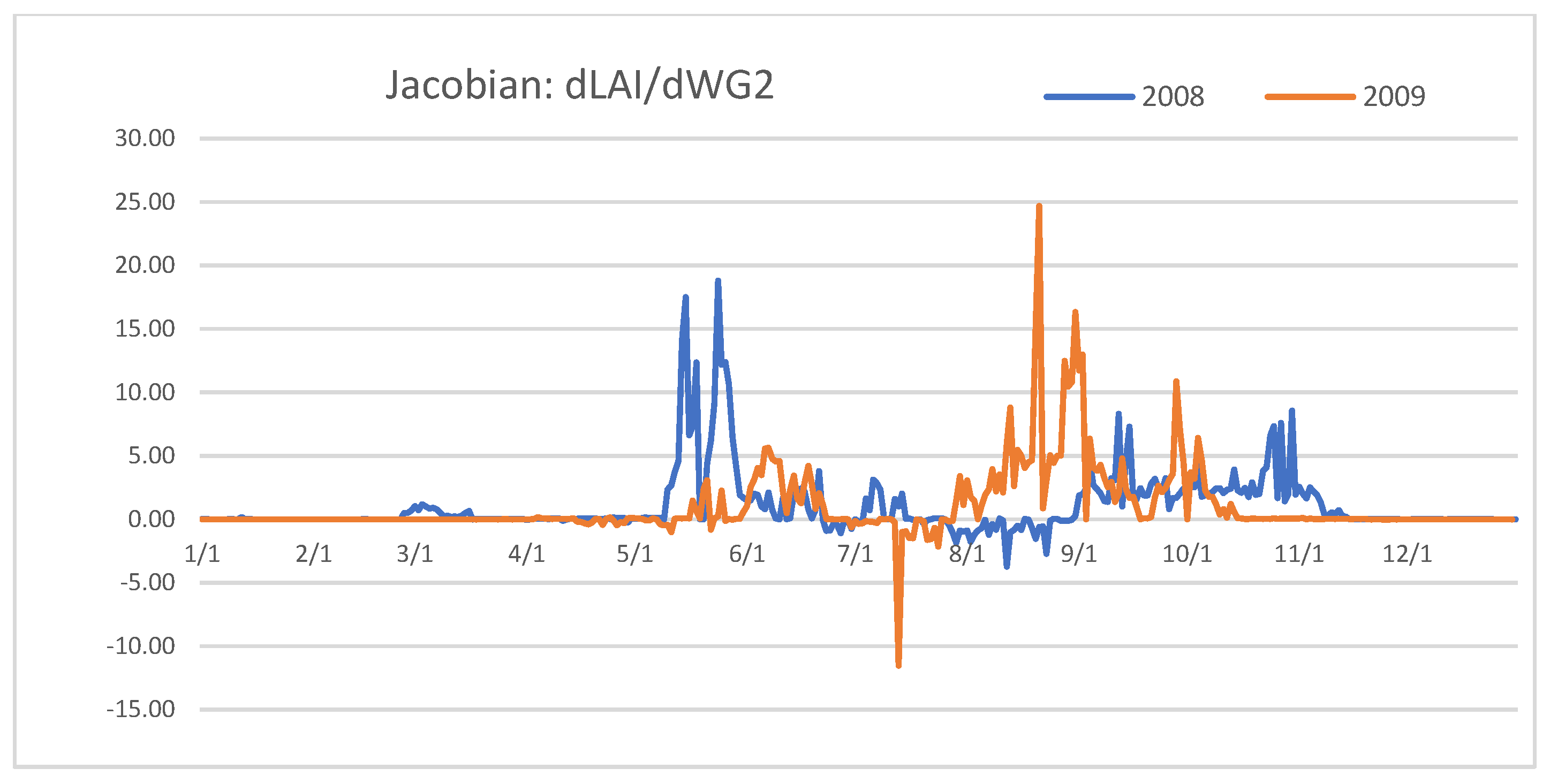
The Jacobian elements are important in order to understand the efficiency of the data assimilation. Figure 4 shows that the dLAI/dWG2 Jacobian term was very variable from year to year. It had generally positive values, but negative values were also found. Small positive perturbation of the root-zone water content directly affected the development and the growing of the plants [7]. Large Jacobians corresponded to the water stress, when WG2 reached the wilting point, a small increase in the WG2 produced a large increase in biomass production. Furthermore, largely positive and negative values might indicate the nonlinearity of the Jacobians. Zero Jacobians occurred during the winter season. Small negative values were generated because the soil water content exceeded the field capacity in these cases.
3.2. Validation
3.2.1. Seasonal Cycle of LAI, WG2, GPP and LE
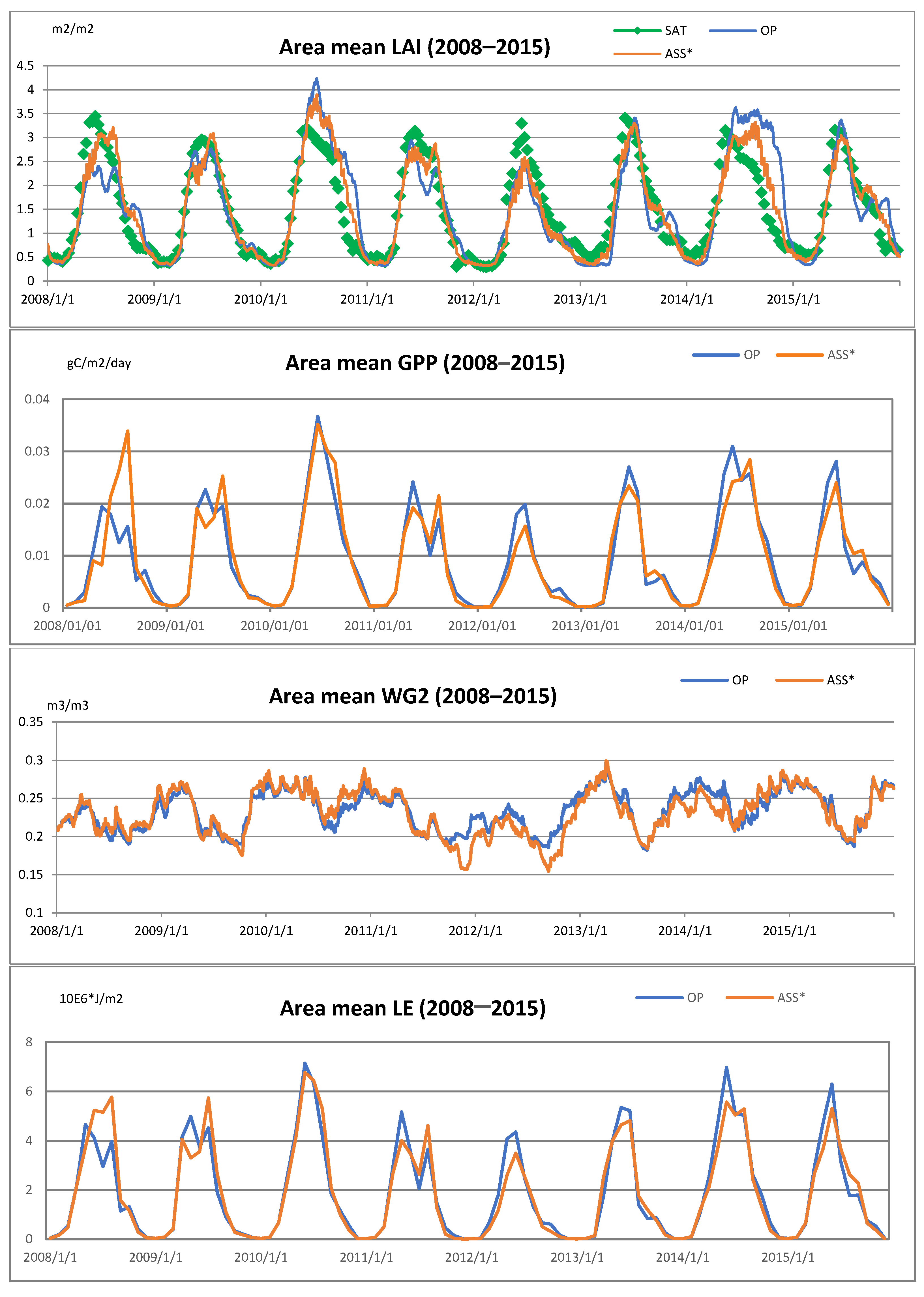
Domain averaged LAI, WG2, GPP, and LE time series are shown in Figure 5 The LAI maximums provided by the satellite did not show such annual variability as simulated by the models. In 2010 the model produced the highest LAI values (Figure 5, first row), about 4 m2/m2, while the satellite had a maximum 3–3.5 m2/m2. In 2010 and in 2014 the models significantly overestimated the LAI values, and the cycle was also longer than for the satellite observations. During these years, large amounts of precipitation fell on the domain, resulting in a longer growing season and higher amounts of above-ground biomass. The vegetation in the model was increased due to heavy rainfall predicted by ALADIN at the beginning of the growing season. The amount of the forecasted precipitation was about twice as much as it was in reality (not shown). All extra precipitation was going to run-off above saturation and did not influence vegetation growth negatively.
The assimilation was able to compensate for differences between the open-loop and the satellite data in 2008, 2011, and 2014. In 2008, LAI values given by the open-loop were underestimated compared to the satellite data, due to hot and dry springs. The assimilation compensated for the lack of biomass, creating larger amounts of GPP and LE flux (Figure 5, second and fourth row). In 2012, there was a drought during the very warm spring and summer seasons, as well as a small amount of precipitation, which resulted in a short cycle by both simulations. GPP, LE was also low, suggesting a lack of vegetation. The precipitation deficits reached 83% of the long-term average and the soil moisture was also kept low, between 0.15–0.22 m3/m3 (Figure 5, third row).
LAI is an important parameter for carbon and water fluxes, but soil moisture also has an important effect on these fluxes. The largest impact on WG2 assimilation was in 2012 and the first half of 2013, resulting in lower GPP and LE values.
Former studies [1,7,8] noted that the beginning of the growing season and the senescence were delayed by the models. In our experiment, the maximum of the growing phase was delayed by the simulations in 2008, 2009, and 2014, and the senescence was shifted in some years (2008, 2010, and 2014).
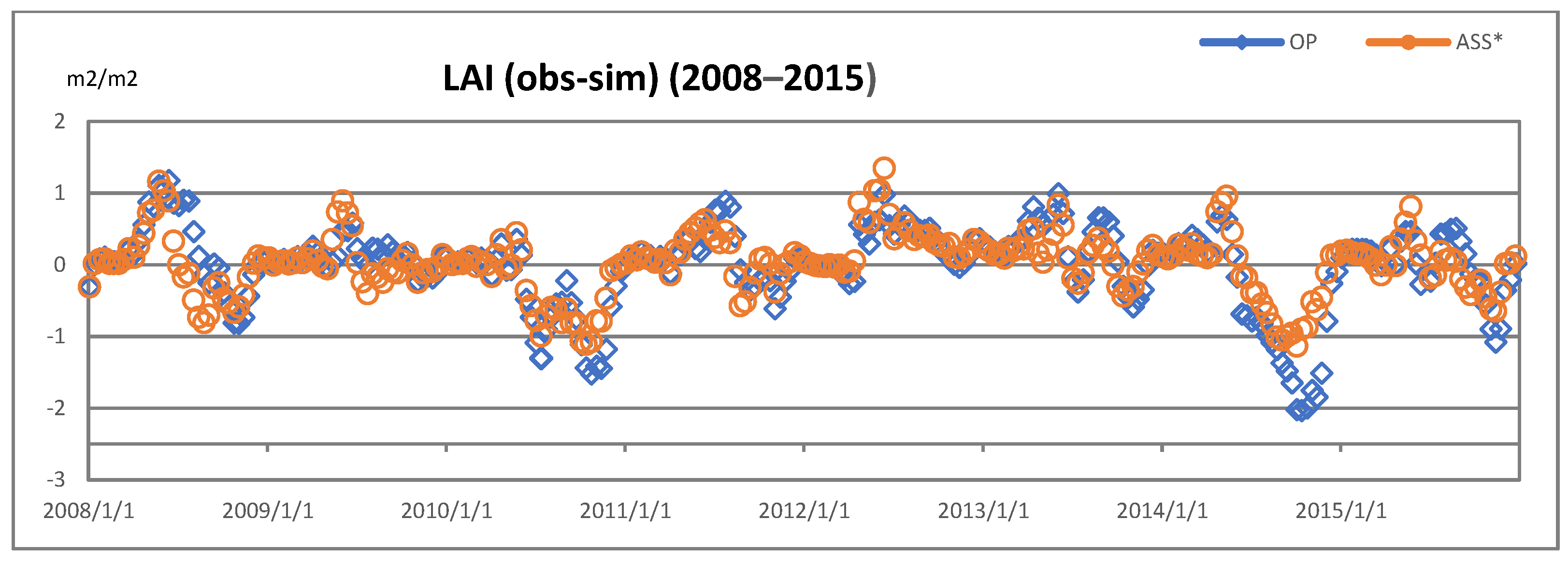
The impact of the assimilation over Hungary was examined with respect to the residuals (differences between the simulations and the satellite observations) for LAI for the period 2008–2015. Figure 6 shows LAI SAT-ASS and SAT-OP points, calculated as the area mean of the entire domain. As expected, LDAS was able to reduce the differences compared to the open-loop simulation. The distribution of the residuals shows seasonal patterns, concentrating at around 0 in winter and increasing for the rest of the year. A large overestimation produced by both simulations (the simulated LAI values exceeded the satellite data) occurred in the wet periods of 2010 and 2014, respectively.
3.2.2. Inter-Annual Variability of LAI and WG2
Drought monitoring is an important area of research nowadays. Our interest was focused on the short-term responses of the vegetation to agricultural drought. The ability of the modeling system to simulate inter-annual variability has also been demonstrated in the Pannonian Basin. Eight years (2008–2015) were simulated using assimilation and open-loop runs. These eight years were used as a baseline for calculating the monthly anomalies for the year 2012 when an extremely severe drought affected Hungary. Most of 2012 was characterised by drought. It was also recorded dry for two months, March, and August, accompanied by severe frosts in February and prolonged heatwaves in summer. The normalised anomaly was calculated as noted in [46]:
where <X> stands for the monthly average and stdev (X) indicates the standard deviation. X can denote variables such as LAI or root-zone soil moisture (WG2), respectively. AnoX could be calculated for monthly or 10-day periods for simulations and satellite data. When the root-zone soil moisture was examined, SWI-10 was used from the satellite, which is a recursive formulation for the exponential filter of SWI over 10 days and correlates well with WG2.
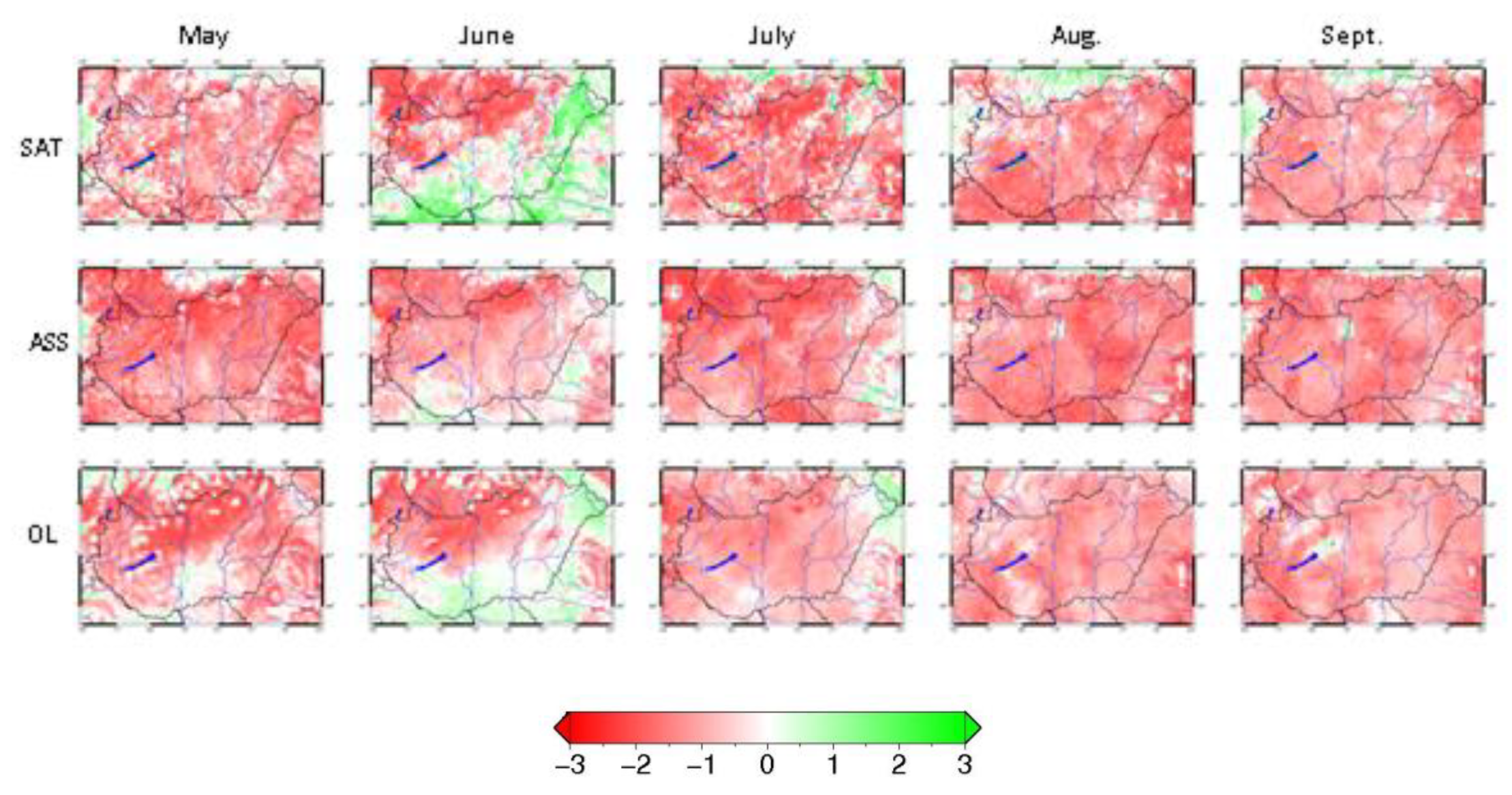
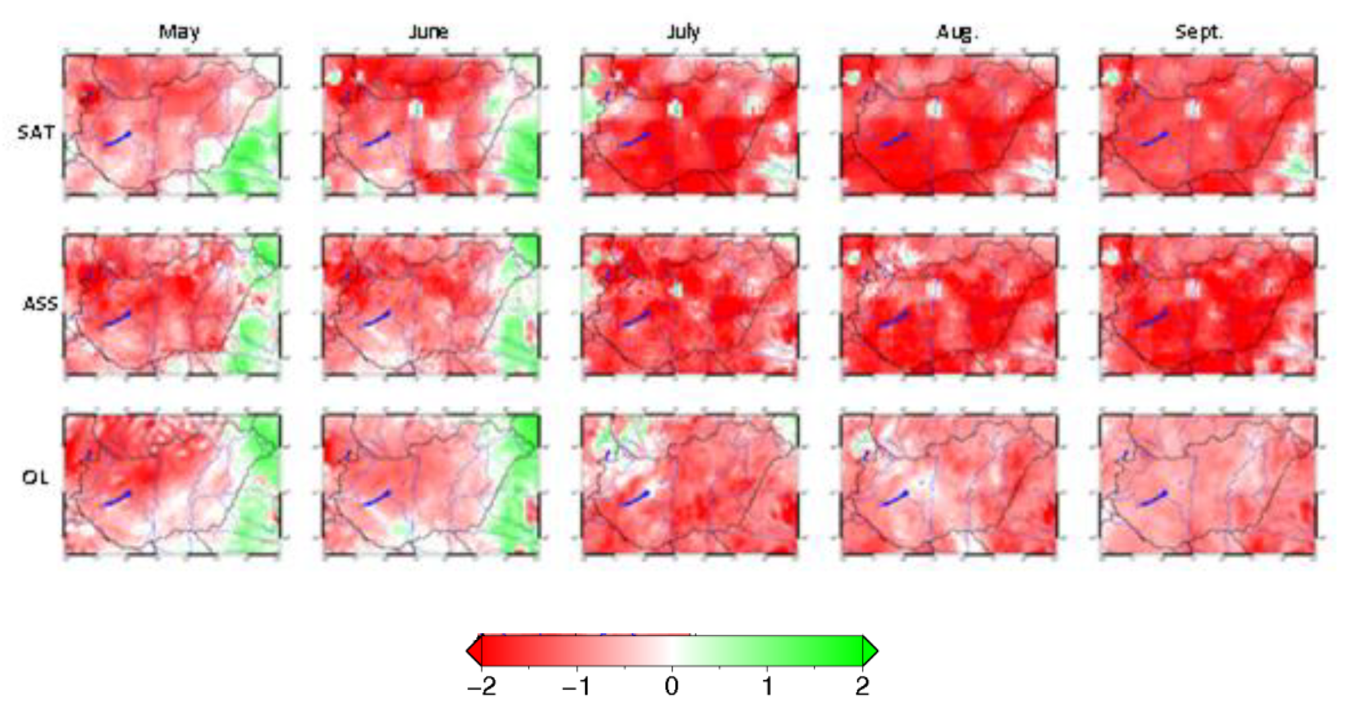
Figure 7 shows monthly AnoLAI values calculated from satellite products and the simulations (open-loop and assimilation). Both experiments were able to reproduce the extremely low LAI anomalies in the summer of 2012, and the root-zone soil moisture anomalies (Figure 8) were represented only by the assimilation run in the summer and autumn of 2012. Higher soil moisture deficits were observed over the Carpathian Basin between July and September by the satellite and assimilation products. In early summer, a positive anomaly was observed in the southern and eastern part of the domain for GEOV1 LAI, while the assimilation was unable to maintain this higher LAI anomaly in these regions. This may be due to a negative anomaly in assimilated WG2 values in spring. The lack of precipitation reached 6% of the March average. Drought occurred at the beginning of the growing phase of the vegetation, which reduced crop productivity.
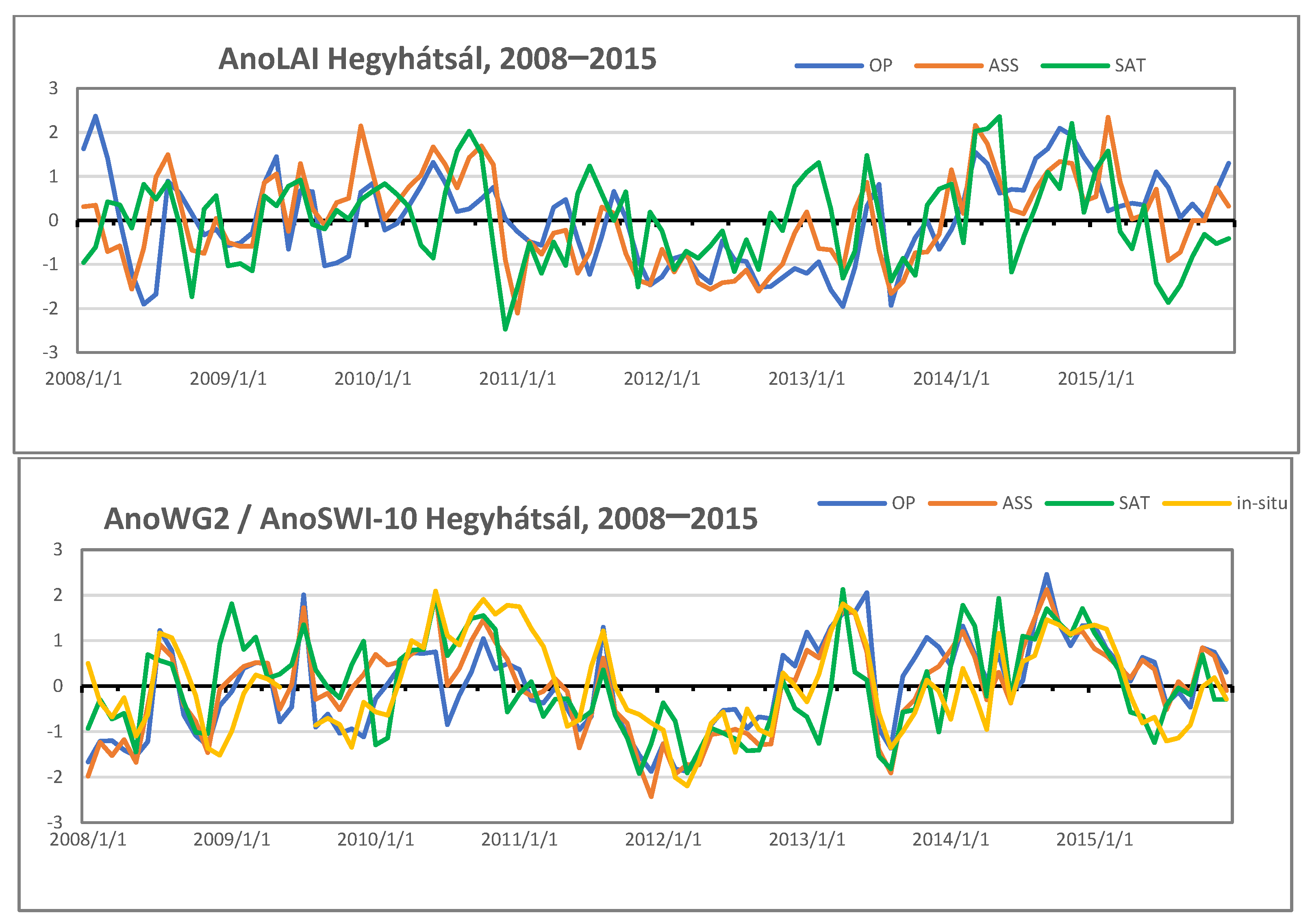
Figure 9 illustrates the time series of AnoLAI and AnoWG2 in Hegyhátsál calculated with LDAS and open-loop model runs as well as satellite and in-situ data. Instead of AnoWG2, AnoSWI-10 was calculated based on the satellite SWI-10 information. AnoWG2 was also determined with the in-situ soil moisture data for Hegyhátsál. The wet years of 2010 and 2014, as well as the drought in 2012, were very well represented by the simulations and the observations. In winter 2013, the AnoLAI values showed opposite behaviors. Satellite values became positive, while the simulated ones were negative over that period. Higher GEOV1 LAI values were noticed in winter and early spring of 2013 (see the mean values on Figure 5, and this was observed at Hegyhátsál by the satellite data (not shown)) compared to the seasonal mean; however, the open-loop run was not able to localise this extreme behavior. At the same time, LDAS was able to compensate by assimilation of LAI. Higher AnoWG2 in-situ series were detected at the beginning of 2008, which did not appear in the rest of the data. In the second half of 2010, heavy precipitation fell in the region, causing high soil moisture anomalies. The simulations were able to follow the processes and capture the maximum values; however, the in-situ measurements showed a wider positive anomaly, while the rest of AnoWG2 data declined rapidly.
3.2.3. Verification of LAI and SWI
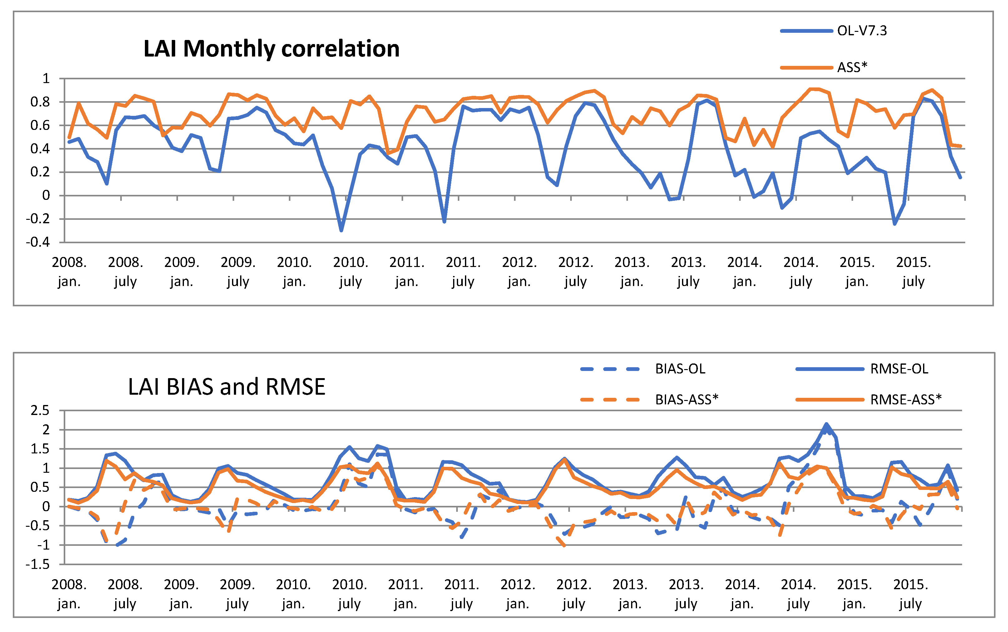
The consistency over time is essential if long-term datasets are assimilated [1]; therefore, anomaly correlation of satellite observation with simulated data was performed for the period 2008–2015. Standard statistics such as correlation, BIAS and RMSE are calculated against the satellite information for both simulations. The monthly area-average LAI and SWI scores are illustrated in Figure 10. Year-to-year correlation ranged within very wide intervals, especially for open-loop simulation. The open-loop experiment produced a low correlation for LAI in every springtime repeatedly, especially in May, and these weak correlations disappeared in the summer or autumn period. In the assimilation, these low correlations did not appear, the extended Kalman filter was relatively stable and worked properly between 0.4 and 0.82 (Figure 10, top). Simulated LAI was controlled by soil moisture, which had high BIAS and RMSE at the beginning of the vegetation period (Figure 10, bottom). Similar to [7], a low correlation was produced by opposite anomalies occurring for some periods where the LAI anomaly in the model was driven by soil moisture over the domain. Besides, the start of the growing season generally occurred later in the model than in the observations. The strong seasonal dependency of the RMSE was notable with 1 m2 m−2 values from May to October. The correlation was also higher in these months. High RMSE and low correlation were achieved in 2014 by open-loop. LAI was underestimated by the simulations (negative bias), especially for the summer months, except for 2010 and 2014, when the amount of biomass was overestimated throughout the year (Figure 10, bottom). Under unusually wet conditions, the biomass production due to photosynthesis was overestimated by ISBA-A-gs.
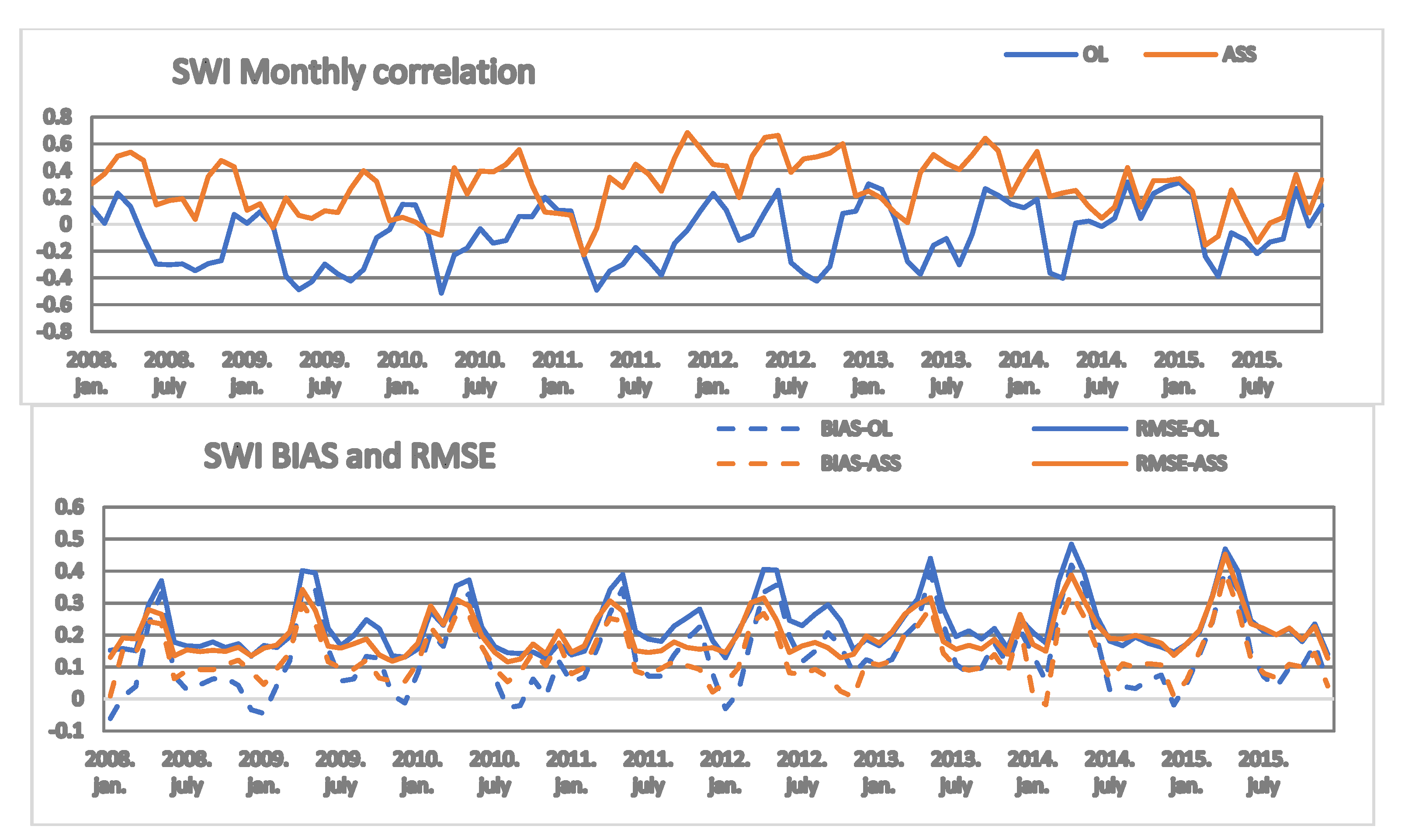
The soil moisture correlation, BIAS, and RMSE of simulated SWI against ASCAT SWI are illustrated in Figure 11, respectively. SWI values were calculated from the simulations using WG2 (root-zone water content): SWI = (WG2 − WG2min)/(WG2max − WG2min), where WG2min and WG2max were obtained from the model results for the period 2008–2015 ASCAT SWI-10 satellite data were used to calculate SWI scores. The weak SWI statistics can be explained by the weak vertical coupling of the model [1]. The assimilation run showed a higher correlation over the entire period compared to the open-loop (Figure 11 top). The improvement of assimilating SWI in the root-zone soil moisture was about 14%, as found in [1]. The RMSE was slightly reduced by the assimilation run, especially in spring periods.
4. Conclusions
A Land Data Assimilation System was developed in Hungary to monitor the above-ground biomass, surface fluxes (carbon and water), and the associated root-zone soil moisture at the regional scale in quasi-real time. It was based on the SURFEX model using the ISBA-A-gs photosynthesis scheme to describe the evolution of vegetation. Our study focused on the ability of the model to describe the inhomogeneity of the ecosystems. Firstly, SURFEX was run in an open-loop mode (i.e., without assimilation) for the period of 2008–2015. Secondly, the Extended Kalman Filter method was used to assimilate SPOT/VGT and PROBA-V LAI and ASCAT/Metop SWI satellite observations. The use of different satellite data at different resolutions challenges for the construction of the EKF observation operator. It was demonstrated in this study that the CDF tool can provide important, meaningful information that makes the observations more suitable for the assimilation.
The comparison generally showed a good agreement between the satellite data and the simulated values for LAI and soil moisture. Both simulations were able to reproduce the variability of the amount of biomass and the soil moisture in different weather situations. The assimilation was able to correct some shortcomings of the open-loop LSM run. It was observed that the maximum of the growing phase was delayed by the simulations, probably because ISBA-A-gs underestimates the photosynthesis in spring. These discrepancies may be partly responsible for a delay of a month in the LAI seasonal cycle. The assimilation significantly reduced this delay and increases the correlation between the model and satellite GEOV1 LAI by more than 0.2–0.3. Due to the high BIAS and RMSE of LAI and WG2, their inter-annual variability was also examined through their scaled anomalies. They were also very well represented by the simulations, especially in the dry summer of 2012. The scaled anomaly can be used as a drought indicator for a period of interest. A regional LDAS system can be used operationally at HMS, and is being developed as follows:
- The results of the assimilation depend on the quality of the data to be assimilated, although the assimilation efficiently corrected LAI high RMSE and BIAS values remained. By applying a finer resolution and assimilating more advanced products of LAI (provided by Sentinel-3/OLCI and PROBA-V) and SWI (provided by Sentinel-1 C-SAR and Metop ASCAT), more precise results can be obtained [47,48]. New types of satellite information can be included in the assimilation system, such as FAPAR, surface albedo, or VOD (Vertical Optical Depth) in the future.
- In this study, the three layers ISBA-A-gs force restore model were used. This means that a single, thick root-zone layer represents soil hydrology, causing a slow response to dry or wet conditions. The propagation of surface soil moisture in the deeper layers may be affected by the lack of vertical resolution of the model. Increasing the number of soil layers allows a more accurate representation of the vertical distribution of soil moisture and the vegetation response to the water stress [1,18,19]. Therefore, the multi-layer version of soil model (diffusion version, ISBA-DIF) is expected to improve the system.
- It is planned that the operational non-hydrostatic AROME NWP forecasts will be corrected by using updated LAI instead of the climatic values. The updated LAI will be provided by daily assimilation of satellite LAI (Sentinel-3). Thus, LDAS should be extended to an AROME Lambert grid with finer 2.5 km resolution.
- The main advantage of LDAS is that it provides a consistent state (analysis) of vegetation and soil variables (moisture and temperature) for a given location and time. This analysis can be used as a starting point for the prediction component of the system, thus implementing a Land Monitoring and Forecasting System. The forecast length depends on the applied atmospheric forcings—the soil and vegetation forecasts can range even up to six months with forcings from ECMWF seasonal predictions. Consequently, the proposed Earth Observation-based information service is not only providing a picture of the current state of soil and vegetation, but is also able to predict the evolution of the vegetation even in seasonal time scale. This capability would make the system attractive for users and stakeholders in the agricultural sector.
Author Contributions
Conceptualization, H.T.; methodology, H.T. and B.S.; software, H.T., B.S.; validation, H.T.; writing—original draft preparation, H.T.; writing—review and editing, H.T. and B.S. All authors have read and agreed to the published version of the manuscript.
Funding
This research was a contribution to the ImagineS project funded by the European Commission under Framework Programme 7 (Grant Agreement No 311766).
Institutional Review Board Statement
Not applicable.
Informed Consent Statement
Not applicable.
Data Availability Statement
The ALADIN and SURFEX ISBA-A-gs simulation data used in this study are stored locally at the Hungarian Meteorological Service. SPOT-VGT, PROBA-V, and ASCAT satellite products were retrieved from European Copernicus Global Land Service (https://land.copernicus.eu/global/, accessed on 21 July 2021). Carbon-, latent heat-flux, LAI, and soil moisture measurements from Hegyhatsal were provided by Eötvös Loránd University in the framework of the ImagineS project and are available upon request.
Acknowledgments
The authors wish to thank László Kullmann for his contribution to the implementation and validation of SURFEX and Gabriella Szépszó for her useful ideas and comments to improve the paper. The authors acknowledge useful discussions with partners in the framework of the PannEx initiative. The authors would like to express their gratitude to the three anonymous reviewers for their detailed and valuable reviews.
Conflicts of Interest
The authors declare no conflict of interest.
References
- Mohr, K.I.; Famiglietti, J.S.; Boone, A.; Starks, P.J. Modeling Soil Moisture and Surface Flux Variability with an Untuned Land Surface Scheme: A Case Study from the Southern Great Plains 1997 Hydrology Experiment. J. Hydrometeorol. 2000, 1, 154–169. [Google Scholar] [CrossRef] [Green Version]
- Viterbo, P. The Representation of Surface Processes in General Circulation Models. Ph.D. Thesis, University of Lisbon, Lisbon, Portuga, 1996; 201p. [Google Scholar]
- Mahfouf, J.F.; Viterbo, P.; Douville, H.; Beljaars, A.; Saarinen, S. A Revised Land-Surface Analysis Scheme in the Integrated Forecasting System. ECMWF Newsl. 2000, 88, 8–13. [Google Scholar]
- Drusch, M.; Scipal, K.; de Rosnay, P.; Balsamo, G.; Andersson, E.; Bougeault, P.; Viterbo, P. Towards a Kalman Filter Based Soil Moisture Analysis System for the Operational ECMWF Integrated Forecast System. Geophys. Res. Lett. 2009, 36. [Google Scholar] [CrossRef]
- Balsamo, G.; Mahfouf, J.F.; Bélair, S.; Deblonde, G. A Land Data Assimilation System for Soil Moisture and Temperature: An Information Content Study. J. Hydrometeorol. 2007, 8, 1225–1242. [Google Scholar] [CrossRef]
- Reichle, R.H.; Walker, J.P.; Koster, R.D.; Houser, P.R. Extended Versus Ensemble Kalman Filtering for Land Data Assimilation. J. Hydrometeorol. 2002, 3, 728–740. [Google Scholar] [CrossRef]
- Barbu, A.L.; Calvet, J.-C.; Mahfouf, J.-F.; Albergel, C.; Lafont, S. Assimilation of Soil Wetness Index and Leaf Area Index Into the Isba-A-Gs Land Surface Model: Grassland Case Study. Biogeosciences 2011, 8, 1971–1986. [Google Scholar] [CrossRef] [Green Version]
- Barbu, A.L.; Calvet, J.-C.; Mahfouf, J.-F.; Lafont, S. Integrating ASCAT Surface Soil Moisture and GEOV1 Leaf Area Index into the SURFEX Modelling Platform: A Land Data Assimilation Application over France. Hydrol. Earth Syst. Sci. 2014, 18, 173–192. [Google Scholar] [CrossRef] [Green Version]
- Albergel, C.; Munier, S.; Leroux, D.J.; Dewaele, H.; Fairbairn, D.; Barbu, A.L.; Gelati, E.; Dorigo, W.; Faroux, S.; Meurey, C.; et al. Sequential Assimilation of Satellite-Derived Vegetation and Soil Moisture Products Using SURFEX_v8.0: LDAS-Monde Assessment over the Euro-Mediterranean Area. Geosci. Model Dev. 2017, 10, 3889–3912. [Google Scholar] [CrossRef] [Green Version]
- Parrens, M.; Mahfouf, J.-F.; Barbu, A.; Calvet, J.-C. Assimilation of Surface Soil Moisture into a Multilayer Soil Model: Design and Evaluation at Local Scale. Hydrol. Earth Syst. Sci. 2014, 18, 673–689. [Google Scholar] [CrossRef] [Green Version]
- Draper, C.S.; Mahfouf, J.-F.; Walker, J.P. An EKF Assimilation of AMSR-E Soil Moisture into the ISBA Land Surface Scheme. J. Geophys. Res. 2009, 114, D20104. [Google Scholar] [CrossRef] [Green Version]
- Draper, C.; Mahfouf, J.-F.; Calvet, J.-C.; Martin, E.; Wagner, W. Assimilation of ASCAT Near-Surface Soil Moisture into the SIM Hydrological Model over France. Hydrol. Earth Syst. Sci. 2011, 15, 3829–3841. [Google Scholar] [CrossRef] [Green Version]
- Rüdiger, C.; Albergel, C.; Mahfouf, J.-F.; Calvet, J.-C.; Walker, J.P. Evaluation of the Observation Operator Jacobian for Leaf Area Index Data Assimilation with an Extended Kalman Filter. J. Geophys. Res. 2010, 115, D09111. [Google Scholar] [CrossRef]
- Mahfouf, J.-F. Assimilation of Satellite-Derived Soil Moisture from ASCAT in a Limited-Area NWP Model. Q. J. Roy. Meteorol. Soc. 2010, 136, 784–798. [Google Scholar] [CrossRef]
- de Rosnay, P.; Drusch, M.; Vasiljevic, D.; Balsamo, G.; Albergel, C.; Isaksen, L. A Simplified Extended Kalman Filter for the Global Operational Soil Moisture Analysis at ECMWF. Q. J. R. Meteorol. Soc. 2013, 139, 1199–1213. [Google Scholar] [CrossRef]
- de Rosnay, P.; Balsamo, G.; Albergel, C.; Munoz-Sabater, J.; Isaken, L. Initialisation of Land Surface Variables for Numerical Weather Prediction. Surv. Geophys. 2014, 35, 607–621. [Google Scholar] [CrossRef]
- Bousetta, S.; Balsamo, G.; Dutra, E.; Beljaars, A.; Albergel, C. Assimilation of Surface Albedo and Vegetation States from Satellite Observations and Their Impact on Numerical Weather Prediction. Remote Sens. Environ. 2015, 163, 111–126. [Google Scholar] [CrossRef] [Green Version]
- Albergel, C.; Munier, S.; Bocher, A.; Bonan, B.; Zheng, Y.; Draper, C.; Leroux, D.J.; Calvet, J.-C. LDAS-Monde Sequential Assimilation of Satellite Derived Observations Applied to the Contiguous US: An ERA-5 Driven Reanalysis of the Land Surface Variables. Remote Sens. 2018, 10, 1627. [Google Scholar] [CrossRef] [Green Version]
- Albergel, C.; Dutra, E.; Munier, S.; Calvet, J.-C.; Munoz-Sabater, J.; de Rosnay, P.; Balsamo, G. ERA-5 and ERA-Interim Driven ISBA Land Surface Model Simulations: Which one performs better? Hydrol. Earth Syst. Sci. 2018, 22, 3515–3532. [Google Scholar] [CrossRef] [Green Version]
- Balsamo, G.; Agusti-Panareda, A.; Albergel, C.; Arduini, G.; Beljaars, A.; Bidlot, J.; Bousserez, N.; Boussetta, S.; Brown, A.; Buizza, R.; et al. Satellite and In Situ Observations for Advancing Global Earth Surface Modelling: A Review. Remote Sens. 2018, 10, 2038. [Google Scholar] [CrossRef] [Green Version]
- Le Moigne, P.; Boone, A.; Calvet, J.-C.; Decharme, B.; Faroux, S.; Gibelin, A.-L.; Lebeaupin, C.; Mahfouf, J.-F.; Martin, E.; Masson, V.; et al. SURFEX Scientific Documentation; Groupe de Météorologie Àmoyenne Échelle, Note de Centre: Meteo-France, Toulouse, 2012; Volume 87, p. 237. [Google Scholar]
- Albergel, C.; Zheng, Y.; Bonan, B.; Dutra, E.; Rodríguez-Fernández, N.; Munier, S.; Draper, C.; de Rosnay, P.; Muñoz-Sabater, J.; Balsamo, G.; et al. Data assimilation for continuous global assessment of severe conditions over terrestrial surfaces. Hydrol. Earth Syst. Sci. 2020, 24, 4291–4316. [Google Scholar] [CrossRef]
- Faroux, S.; Kaptue Tchuente, A.T.; Roujean, J.-L.; Masson, V.; Martin, E.; Le Moigne, P. ECOCLIMAP-II/Europe: A Twofold Database of Ecosystems and Surface Parameters at 1 km Resolution Based on Satellite Information for Use in Land Surface, Meteorological and Climate Models. Geosci. Model. Dev. 2013, 6, 563–582. [Google Scholar] [CrossRef] [Green Version]
- Noilhan, J.; Planton, S. A Simple Parameterization of Land Surface Processes for Meteorological Models. Mon. Weather. Rev. 1989, 117, 536–549. [Google Scholar] [CrossRef]
- Noilhan, J.; Mahfouf, J.-F. The ISBA Land Surface Parameterisation Scheme. Glob. Planet. Chang. 1996, 13, 145–149. [Google Scholar] [CrossRef]
- Calvet, J.-C.; Noilhan, J.; Roujean, J.-L.; Bessemoulin, P.; Cabelguenne, M.; Olioso, A.; Wigneron, J.-P. An Interactive Vegetation SVAT Model Tested Against Data from Six Contrasting Sites. Agric. For. Meteorol. 1998, 92, 73–95. [Google Scholar] [CrossRef]
- Gibelin, A.-L.; Calvet, J.-C.; Roujean, J.-L.; Jarlan, L.; Los, S.O. Ability of the Land Surface Model ISBA-A-Gs to Simulate Leaf Area Index at the Global Scale: Comparison with Satellites Products. J. Geophys. Res. 2006, 111, D18102. [Google Scholar] [CrossRef]
- Calvet, J.-C.; Lafont, S.; Cloppet, E.; Souverain, F.; Badeau, V.; Le Bas, C. Use of Agricultural Statistics to Verify the Interannual Variability in Land Surface Models: A Case Study over France with ISBA-A-Gs. Geosci. Model. Dev. 2012, 5, 37–54. [Google Scholar] [CrossRef] [Green Version]
- Canal, N.; Calvet, J.-C.; Decharme, B.; Carrer, D.; SLafont, S.; Pigeon, G. Evaluation of Root Water Uptake in the ISBA-A-Gs Land Surface Model Using Agricultural Yield Statistics over France. Hydrol. Earth Syst. Sci. 2014, 18, 4979–4999. [Google Scholar] [CrossRef] [Green Version]
- Horányi, A.; Kertész, S.; Kullmann, L.; Radnóti, G. The ARPEGE/ALADIN Mesoscale Numerical Modelling System and its Application at the Hungarian Meteorological Service. Időjárás 2006, 110, 203–227. [Google Scholar]
- Horányi, A.; Ihász, I.; Radnóti, G. ARPEGE/ALADIN: A Numerical Weather Prediction Model for Central-Europe with the Participation of the Hungarian Meteorological Service. Időjárás 1996, 100, 277–301. [Google Scholar]
- Mile, M.; Bölöni, G.; Randriamampianina, R.; Steib, R.; Kucukkaraca, E. Overview of Mesoscale Data Assimilation Developments at the Hungarian Meteorological Service. Időjárás 2015, 119, 215–239. [Google Scholar]
- Baret, F.; Weiss, M.; Lacaze, R.; Camacho, F.; Makhmara, H.; Pacholczyk, P.; Smets, B. GEOV1: LAI and FAPAR Essential Climate Variables and FCover Global Times Series Capitalizing over Existing Products. Part1: Principles of Development and Production. Remote Sens. Environ. 2013, 137, 299–309. [Google Scholar] [CrossRef]
- Camacho, F.; Cernicharo, J.; Lacaze, R.; Baret, F.; Weiss, M. GEOV1: LAI, FAPAR Essential Climate Variables and FCover Global Time Series Capitalizing over Existing Products. Part 2: Validation and Inter-Comparison with Reference Products. Remote Sens. Environ. 2013, 137, 310–329. [Google Scholar] [CrossRef]
- Albergel, C.; Rüdiger, C.; Pellarin, T.; Calvet, J.-C.; Fritz, N.; Froissard, F.; Suquia, D.; Petitpa, A.; Piguet, B.; Martin, E. From Near-Surface to Root-Zone Soil Moisture Using an Exponential Filter: An Assessment of the Method Based on In-Situ Observations and Model Simulations. Hydrol. Earth Syst. Sci. 2008, 12, 1323–1337. [Google Scholar] [CrossRef] [Green Version]
- Albergel, C.; Rüdiger, C.; Carrer, D.; Calvet, J.-C.; Fritz, N.; Naeimi, V.; Bartalis, Z.; Hasenauer, S. An Evaluation of ASCAT Surface Soil Moisture Products with In-Situ Observations in Southwestern France. Hydrol. Earth Syst. Sci. 2009, 13, 115–124. [Google Scholar] [CrossRef] [Green Version]
- Reichle, R.H.; Koster, R.D. Bias Reduction in Short Records of Satellite Soil Moisture. Geophys. Res. Lett. 2004, 31, L19501. [Google Scholar] [CrossRef] [Green Version]
- Pastorello, G.; Trotta, C.; Canfora, E.; Chu, H.; Christianson, D.; Cheah, Y.W.; Poindexter, C.; Chen, J.; Elbashandy, A.; Humphrey, M.; et al. The FLUXNET2015 Dataset and the ONEFlux Processing Pipeline for Eddy Covariance Data. Sci. Data 2020, 7, 225. [Google Scholar] [CrossRef]
- FLUXNET Datasets List. Available online: https://fluxnet.ornl.gov/site/505 (accessed on 21 July 2021).
- Nagy, Z.; Pintér, K.; Czóbel, S.Z.; Balogh, J.; Horváth, L.; Fóti, S.Z.; Barcza, Z.; Weidinger, T.; Csintalan, Z.S.; Dinh, N.Q.; et al. The Carbon Budget of Semi-Arid Grassland in a Wet and a Dry Year in Hungary. Agric. Ecosyst. Environ. 2007, 121, 21–29. [Google Scholar] [CrossRef]
- Barcza, Z.; Haszpra, L.; Kondo, H.; Saigusa, N.; Yamamoto, S.; Bartholy, J. Carbon Exchange of Grass in Hungary. Tellus B 2003, 55, 187–196. [Google Scholar] [CrossRef]
- Haszpra, L.; Hidy, D.; Taligás, T.; Barcza, Z. First Results of Tall Tower Based Nitrous Oxide Flux Monitoring over an Agricultural Region in Central Europe. Atmos. Environ. 2018, 176, 240–251. [Google Scholar] [CrossRef]
- Scipal, K.; Drusch, M.; Wagner, W. Assimilation of a ERS Scatterometer Derived Soil Moisture Index in the ECMWF Numerical Weather Prediction System. Adv. Water Resour. 2008, 31, 1101–1112. [Google Scholar] [CrossRef]
- Bouttier, F.; Courtier, P. Data Assimilation Concepts and Methods. In Meteorological Training Course Lecture Series; ECMWF: Reading, UK, 1999; 75p. [Google Scholar]
- Fairbairn, D.; Barbu, A.L.; Napoly, A.; Albergel, C.; Mahfouf, J.-F.; Calvet, J.-C. The Effect of Satellite-Derived Surface Soil Moisture and Leaf Area Index Land Data Assimilation on Streamflow Simulations over France. Hydrol. Earth Syst. Sci. 2017, 21, 2015–2033. [Google Scholar] [CrossRef] [Green Version]
- Szczypta, C.; Calvet, J.-C.; Maignan, F.; Dorigo, W.; Baret, F.; Ciais, P. Suitability of Modelled and Remotely Sensed Essential Climate Variables for Monitoring Euro-Mediterranean Droughts. Geosci. Model. Dev. 2014, 7, 931–946. [Google Scholar] [CrossRef] [Green Version]
- Fuster, B.; Sánchez-Zapero, J.; Camacho, F.; García-Santos, V.; Verger, A.; Lacaze, R.; Weiss, M.; Baret, F.; Smets, B. Quality Assessment of PROBA-V LAI, fAPAR and fCOVER Collection 300 m Products of Copernicus Global Land Service. Remote Sens. 2020, 12, 1017. [Google Scholar] [CrossRef] [Green Version]
- Bauer-Marschallinger, B.; Paulik, C.; Hochstöger, S.; Mistelbauer, T.; Modanesi, S.; Ciabatta, L.; Massari, C.; Brocca, L.; Wagner, W. Soil Moisture from Fusion of Scatterometer and SAR: Closing the Scale Gap with Temporal Filtering. Remote Sens. 2018, 10, 1030. [Google Scholar] [CrossRef] [Green Version]
Figure 1.
Raw (a) and extrapolated (b) GEOV1 Leaf area index from the Copernicus Global Land Service project on 13 April 2008.
Figure 1.
Raw (a) and extrapolated (b) GEOV1 Leaf area index from the Copernicus Global Land Service project on 13 April 2008.

Figure 2.
Surface soil moisture evolutions for 2008 at Hegyhátsál (West-Hungary) for model (red), raw ASCAT satellite observations (purple) and ASCAT seasonal CDF rescaled (blue) observations.
Figure 2.
Surface soil moisture evolutions for 2008 at Hegyhátsál (West-Hungary) for model (red), raw ASCAT satellite observations (purple) and ASCAT seasonal CDF rescaled (blue) observations.

Figure 3.
Location of the monitoring site at Hegyhátsál.

Figure 4.
Jacobian values of dLAI/dWG2 for 2008 and 2009.

Figure 5.
Time series of open-loop (blue), observed (green) and assimilation (orange) LAI (first row), GPP (second row), WG2 (third row), and LE (fourth row) averaged over Hungary from 2008 to 2015.
Figure 5.
Time series of open-loop (blue), observed (green) and assimilation (orange) LAI (first row), GPP (second row), WG2 (third row), and LE (fourth row) averaged over Hungary from 2008 to 2015.

Figure 6.
Time series of the residuals, SAT-OP: blue, SAT-ASS*: orange.

Figure 7.
Monthly anomalies for the year 2012 from May to September: GEOV1 LAI product (first row), assimilated LAI (second row) and open-loop LAI (third row).
Figure 7.
Monthly anomalies for the year 2012 from May to September: GEOV1 LAI product (first row), assimilated LAI (second row) and open-loop LAI (third row).

Figure 8.
Monthly anomalies for the year 2012 from May to September: ASCAT/SWI-10 product (first row) assimilated WG2 (second row) and open-loop WG2 (third row).
Figure 8.
Monthly anomalies for the year 2012 from May to September: ASCAT/SWI-10 product (first row) assimilated WG2 (second row) and open-loop WG2 (third row).

Figure 9.
AnoLAI and AnoWG2/AnoSWI-10 time series for 2008–2015 at Hegyhátsál (OL: blue, ASS: orange, GEOV1 LAI and SWI-10: green, in-situ: yellow).
Figure 9.
AnoLAI and AnoWG2/AnoSWI-10 time series for 2008–2015 at Hegyhátsál (OL: blue, ASS: orange, GEOV1 LAI and SWI-10: green, in-situ: yellow).

Figure 10.
Seasonal correlation (top); BIAS (bottom, dashed line) and RMSE (bottom full line)) for LAI for open-loop (blue) and assimilation (orange) runs.
Figure 10.
Seasonal correlation (top); BIAS (bottom, dashed line) and RMSE (bottom full line)) for LAI for open-loop (blue) and assimilation (orange) runs.

Figure 11.
Seasonal correlation (top); BIAS (bottom, dashed line) and RMSE (bottom, full line)) for SWI for open-loop (blue) and assimilation (orange) runs.
Figure 11.
Seasonal correlation (top); BIAS (bottom, dashed line) and RMSE (bottom, full line)) for SWI for open-loop (blue) and assimilation (orange) runs.


Table 1.
Experimental setup of this study.
| Name of Experiment | Model | Domain | Atmospheric Forcing | Data Assimilation Method | Assim. Observations | Control Variables | Time Period | Model Outputs |
|---|---|---|---|---|---|---|---|---|
| Open-loop | SURFEX, ISBA-A-gs | Carpathian Basin | ALADIN, LandSAF | - | - | - | 2008–2015 (2007 spin up) | LAI, WG2, GPP, NEE, LE |
| LDAS | SURFEX, ISBA-A-gs | Carpathian Basin | ALADIN, LandSAF | EKF | ASCAT SWI SPOT/VGT and PROBA-V LAI | WG1, WG2 and LAI | 2008–2015 (2007 spin up) | LAI, WG2, GPP, NEE, LE |
Publisher’s Note: MDPI stays neutral with regard to jurisdictional claims in published maps and institutional affiliations. |
© 2021 by the authors. Licensee MDPI, Basel, Switzerland. This article is an open access article distributed under the terms and conditions of the Creative Commons Attribution (CC BY) license (https://creativecommons.org/licenses/by/4.0/).
Share and Cite
MDPI and ACS Style
Tóth, H.; Szintai, B. Assimilation of Leaf Area Index and Soil Water Index from Satellite Observations in a Land Surface Model in Hungary. Atmosphere 2021, 12, 944. https://0-doi-org.brum.beds.ac.uk/10.3390/atmos12080944
AMA Style
Tóth H, Szintai B. Assimilation of Leaf Area Index and Soil Water Index from Satellite Observations in a Land Surface Model in Hungary. Atmosphere. 2021; 12(8):944. https://0-doi-org.brum.beds.ac.uk/10.3390/atmos12080944
Chicago/Turabian StyleTóth, Helga, and Balázs Szintai. 2021. "Assimilation of Leaf Area Index and Soil Water Index from Satellite Observations in a Land Surface Model in Hungary" Atmosphere 12, no. 8: 944. https://0-doi-org.brum.beds.ac.uk/10.3390/atmos12080944
Note that from the first issue of 2016, this journal uses article numbers instead of page numbers. See further details here.