Article

Reconciling Reduced Red Meat Consumption in Canada with Regenerative Grazing: Implications for GHG Emissions, Protein Supply and Land Use

by
James A. Dyer
1,* and
Raymond L. Desjardins
2
1
Agriculture and Agri-Food Canada, 122 Hexam Street, Cambridge, ON N3H 3Z9, Canada
2
Science and Technology Branch, Agriculture and Agri-Food Canada, Government of Canada, 960 Carling Avenue, Ottawa, ON K1A 0C6, Canada
*
Author to whom correspondence should be addressed.
Submission received: 31 May 2021 / Revised: 25 June 2021 / Accepted: 8 July 2021 / Published: 23 July 2021
(This article belongs to the Special Issue Agricultural Greenhouse Gas Emissions)

Abstract

:
This paper reconciled the soil ecology benefits of forages and ruminants with reducing GHG emissions from beef. A scenario analysis compared four integrated systems for beef, pork and broilers. Slaughter cattle diets were either business as usual (BAU) or grass fed (GF), and the combined red meat consumption could not exceed the recommendation for human health. The four consumption scenarios included (PS1) equal beef and pork with BAU beef, (PS2) equal beef and pork with GF beef, (PS3) more pork and less beef with GF beef and (PS4) more pork and less beef with BAU beef. Broiler consumption was increased to force all four scenarios to provide the same amount of protein. All four scenarios required similar feed grain areas (2.5 to 3 Mha). At 2.3, 4.4, 2.2 and 1.2 Mha for PS1, PS2, PS3 and PS4, respectively, the areas in harvestable forage showed much greater variation. From high to low GHG emissions, the ranking of scenarios was PS2, PS1, PS3 and PS4. Although allowing for avoidance of soil organic matter loss changed this ranking, the carbon footprint of beef production was still double or more that of pork in all four PS. To reconcile the agro-ecological benefits of beef with reducing GHG emissions, PS3 may be better than PS4. Along with eating more pork and broilers, and less red meat overall, consumers can choose GF beef as an occasional alternative.

Graphical Abstract

1. Introduction

Defining the role that livestock should play in producing the food needed for a world populated by 11 billion people is one of the great challenges facing humanity in the 21st century [1,2,3]. While some experts argue that ruminants are essential for sustainable land use, others insist that reducing enteric methane emissions is a critical step towards fighting climate change. The goal of this paper was to determine whether these two land use approaches can be reconciled for the beef industry. Because of the imperative of food production [4], particularly protein [1], understanding agricultural land use change is as important to this reconciliation as the carbon footprint of the sector. This paper will assess the potential land use changes that might accompany the shifts in the Canadian beef industry that many experts are calling for, along with the carbon footprints of these two production systems.
Reducing agricultural greenhouse gas (GHG) emissions must be part of any serious plan to combat climate change [3,5,6,7]. Agriculture contributes about half of the global nitrous oxide and methane emissions [8]. The GHG emissions from the ruminant livestock industries rival the fossil CO2 emissions from transportation [9,10]. Many agricultural soils, which cover 35% to 40% of the Earth’s ice-free land area [4,11], have lost between one third and three quarters of their organic carbon [12,13]. Food production (from field to plate) accounts for a quarter of the global CO2 emissions [14]. The expanding need for land to support livestock, and the associated impacts on water, biodiversity and GHG emissions, combined with climate change, has been called a “perfect storm” [2].
Human demand for animal protein is expected to increase over the next few decades due to population growth and rising per capita consumption [1,15]. A handful of countries, including Canada, are eating too much meat at the expense of the rest of the world [14,16] and meat production in North America has become highly intensive [17]. The impacts of Canada’s food consumption habits are 4.5 times as high as Canada’s rightful share of the planetary climate boundary for food [14]. Of 20 countries compared, Hood [14] ranked Canada as the seventh poorest performer on this scale.

1.1. Combatting Climate Change through Reduced Methane Emissions

Many experts have taken the position that livestock, particularly ruminants, contribute disproportionally to global warming compared to other food sources [18,19,20]. Beef has been identified as a major source of GHG [7,17] and reductions in ruminant populations could make a substantial contribution to reducing climate change [1,20,21]. Eating less red meat could reduce GHG emissions more than abandoning our cars [9]. Because about a third of all crops are grown for livestock feed, much of the GHG emissions from crop production are actually driven by livestock [11]. In Canada almost half of the total crop land was determined to be in the livestock crop complex [22].
Although consumption is driving these GHG emissions [1], it is difficult for consumers to understand how their eating habits can affect the climate [5,17]. Nevertheless, part of the solution to the carbon footprint of our food system would be to reduce the demand for animal products [11,21]. The livestock reductionists have recently been gifted a supporting argument from the medical community, with many from that community calling for reduced red meat consumption to improve public health [23,24,25]. The commodity that is subject to both imperatives, being both a ruminant and red meat, is beef [23], which accounts for 60% of the GHG emissions from Canadian livestock [26]. Therefore, if red meat consumption in Canada was substantially reduced, both the environment and the health of Canadians could see substantial improvements [27,28].

1.2. Combatting Climate Change through Regenerative Agriculture

Organic agriculture, including livestock production, could help to minimize climate change [2,8,29]. Much of the solution involves treating the soil as a carbon sink [6,30,31]. Regenerative agriculture is a farm management style that does not just sustain the land; it improves it for future generations [32,33]. The principles of regenerative agriculture include minimizing soil disturbance and chemical inputs, maximizing biodiversity and keeping the soil covered [7,32]. Among other agro-ecological benefits, regenerative agriculture increases soil structure, soil biodiversity [34] and organic matter [32], which promote carbon sequestration [12,31,35].
Kenyon [36] defined perennial forage management practices that emphasize long term over short term production as regenerative grazing. These practices can reduce the carbon footprint of agriculture [32,33,37]. As well as maintaining soil organic carbon [13,31,37], incorporating forages and ruminants into agroecosystems can improve soil ecological functions [7,34,38]. The grass-fed movement insists that ruminants are essential to a healthy ecosystem [39]. Some believe that grazing practices can stimulate grass root growth to store enough soil organic carbon to offset the methane emissions of the grazing animals [11]. Although such practices can include rotational grazing [1,3], there is concern as to whether the rotational approach to grazing is always more effective than, or as ecologically beneficial as, simply maintaining sustainable stocking rates [21,40].
For cattle on pasture, all of their manure is deposited directly on the land for which the methane emissions are negligible compared to cattle in confined paddocks or feedlots [41]. Although manure can still be spread mechanically as fertilizer on hay fields, this consumes some fossil fuel and requires storage prior to spreading, which leads to manure methane emissions [42]. However, these additional GHG emissions were taken into account by Vergé et al. [41,43]. Both pasture and hay fields require less chemical fertilizer, another GHG source, than annual grain crops [32]. Regardless, ruminants are still the only way to convert cellulose into usable protein for humans [42,44].

1.3. Potential Limits of Regenerative Agriculture

Advocates of regenerative agriculture as a tool to control climate change must also be mindful of some of its limitations. For example, because soils are carbon sinks, they eventually become saturated [30], whereas GHG emissions are annual fluxes, which makes the two difficult to compare [38,43]. Additionally, removing CO2 from the atmosphere can take years, or even decades, whereas reducing annual GHG emission takes effect immediately [11], thus addressing the urgency of the climate crisis. Natural ecosystems should not be converted to agricultural land solely for sequestering carbon [11].
GHG emission intensities associated with grazing cattle are higher than from the feedlot system because of the larger slaughter animals in feedlots and their shorter lives [39], as well as their low roughage diets [6,45,46,47] and shelter from weather stress [46,48]. Pastureland can also be damaged by over-stocking [49]. Due to the emphasis on long term agroecosystem health and less intensive meat production, beef produced by regenerative grazing will provide a smaller portion of Canada’s domestic supply of carcass protein [36]. Hence, unless farmers can diversify their income sources, regenerative agriculture may require that they charge a higher price for their meat products to realize a viable living [32]. From a global perspective, such diversification will likely make complete (animal quality) protein less available to the human food chain [13], unless alternative sources are identified.

2. Materials and Methods

Although the arguments made for regenerative agriculture and reduced red meat consumption are largely contradictory, they are both compelling. This divergence motivated the goal of this paper: to determine whether these two positions can be reconciled for the Canadian beef industry. Regenerative agriculture for the beef industry means regenerative grazing. For the purpose of this analysis, all rearing of cattle on perennial forage is considered regenerative compared to using annual crops as cattle feed, even if that perennial forage is mechanically harvested. Although the diet for most beef cattle in Canada is predominantly forage, most Canadian slaughter cattle are finished for market in feedlots on a high feed grain diet [41]. With the need to keep soil covered year-round [7,32], the first step in the transition to regenerative grazing must involve less dependence on feed grains. In temperate climates like Canada, where grazing is seasonal, grass forage must be stored for winter feed as hay [50]. Therefore, reducing feed grain dependence to avoid soil carbon loss to the atmosphere [31] would require an increase in harvestable perennial (grass) forage.
Along with 2.0 Mha of feed grains and 6.1 Mha of harvestable forage, the 2001 Canadian beef crop complex included 4.3 Mha of seeded pasture [41]. The main role of pastureland, including both seeded pasture and rangeland, is to maintain the breeding cows and young calves [24,51]. Although rangeland has only marginal grazing value in Canada [51], up to 11 Mha of rangeland [51,52] are available to maintain the breeding herd. However, the feed value of both pastureland areas is difficult to quantify [41,43]. Rangeland, in particular, is also (by definition) land that cannot support annual crops [53]. Nevertheless, a big enough increase in the harvested forage needed for slaughter cattle could either increase the stocking rates on seeded pasture or lead to greater dependence on rangeland to maintain the breeding cows and calves. Either of these outcomes would impede the basic principles of regenerative grazing [36,49,54].
Given how much Canada is exceeding its share of the planetary climate boundary for food [14], the scope of this examination will be limited to Canada. Since all livestock industries exist to supply the complete protein necessary for the human diet [55,56], livestock production will likely continue for the foreseeable future. Therefore, the only protein alternatives considered here will be from livestock. Because of the impact of beef on Canada’s GHG emissions [26,43] and its role in providing protein to the human food chain [56,57], the GHG-protein indicator [18] will be an important metric in this analysis, and recent findings from that indicator [23,24,27] will be taken as a starting point. However, land use will be the major determinant in reaching this reconciliation goal.
Table 1 provides a roadmap through this analysis using the tables and figures as landmarks. The first five stages (left side) identify the major contributions from previous work to this analysis. Stages 2 to 4 introduce the components of the scenario analysis model. By separating beef into two separate commodities based on diet, Stage 5 is the starting point of the calculations specific to this paper. Although Stage 6 did not contribute directly to the goal of this analysis, the validation of area differences between the two beef diet scenarios was crucial to Stage 7, which then set up Stage 8 to introduce and quantify the potential role of avoided soil carbon loss in the scenario analysis.

2.1. The GHG-Protein Indicator

Much of the work in Canada towards minimizing the carbon footprint of Canadian agriculture has focused on comparing the GHG emission budgets of Canadian livestock industries, namely beef, pork, dairy, poultry and sheep [41,58,59,60,61] based on livestock feed intake data [62]. Dyer et al. [18] compared the GHG emission budgets of beef, pork, dairy and poultry on the basis of protein. The GHG-protein indicator was used by three other research teams to report the GHG–protein ratios for livestock on an international scale [63,64,65]. The broadest ranges were in beef, mainly because they reflect many different beef production systems adapted to a diversity of environments [42]. However, the differences in these ratios among beef, pork and poultry were similar to those reported by Dyer et al. [18]. Nijdam et al. [65] separated beef industries into intensive and extensive systems, with extensive systems having roughly 20% higher GHG–protein ratios than the intensive systems.

2.1.1. Canadian Applications of the GHG-Protein Indicator

Between 2012 and 2018, the GHG-protein indicator saw a number of other applications in Canada, including: redistribution of beef and pork populations to quantify different payback periods for soil carbon [43]; as a basis for displacing some beef cattle with sheep [61]; to assess co-grazing sheep and beef in Western Canadian rangeland [51]; and to compare two ruminants (beef and dairy) to two non-ruminants (pork and poultry) on an east-west basis [66]. In order to assess the impact of Canola meal as ruminant livestock feed, Dyer et al. [67] assumed a fixed quantity of protein production for two scenarios for feeding Canola meal to sheep and beef cattle. The GHG-protein indicator was used to compare pulse and livestock (both ruminants and non-ruminants) as protein sources [68]. Both the direct and reciprocal forms of the GHG-protein indicator were used to compare GHG emissions from ruminant and non-ruminant livestock on eco-district and provincial scales [69]. Desjardins et al. [70] presented a graphical summary of livestock differences, recently updated by Dyer and Desjardins [27], of the GHG emissions per kg of the protein from six livestock commodities.

2.1.2. National Protein Intake and Red Meat

With the attention drawn to diversifying protein sources by the 2019 Canada Food Guide, Dyer et al. [23,24] applied the GHG-protein indicator to the medical concern for excessive red meat (RM) consumption [25]. The medical recommendation to eat less RM to reduce heart- and cancer-related health risks was used by Dyer et al. [23] as a proxy for qualitative guidance from the 2019 Food Guide [71]. The medical recommendations were integrated with several possible responses by livestock producers in a scenario analysis. Dyer et al. [24] highlighted the potential role of Canadian consumers in influencing crop and livestock management and land use decisions. Both of these papers applied the same protein supply boundary condition form of the indicator first used by Dyer et al. [67].
The algorithm used by Dyer et al. [23,24] selected beef and pork to represent Canadian RM, while increasing the consumption of broilers (to represent non-RM protein) in order to maintain the national protein intake (NPI). Hence, the GHG emission calculations had an upper boundary condition of recommended RM consumption and a lower boundary condition defined by maintaining NPI as the total protein from the beef, pork and broilers consumed in Canada in 2017. Most previous uses of this indicator applied the GHG protein ratio as part of a suite of performance indicators. However, by expanding broilers to maintain NPI, this algorithm treated protein as an objective function. Figure 1 (modified from Dyer and Desjardins [27]) shows how the two boundary conditions set the limits of the GHG emission calculations from the three commodities.
The smaller box in Figure 1 shows (somewhat counter-intuitively) the upper boundary condition that forces beef and pork consumption to stay at or below the medically recommended RM. The larger box in Figure 1 shows the lower boundary condition for keeping total protein at or above NPI. The upward pointing arrows represent the required expansion of broiler consumption to satisfy the objective function. Protein from all three commodities (gray) is expressed as the boneless weight equivalent of RM. Both boundary conditions apply to two pairs of simulations (a and b). The downward arrow from RM(C) to the RM boundary condition (small box) was the average of the three medically based reduction scenarios for the consumption (C) of RM [23].

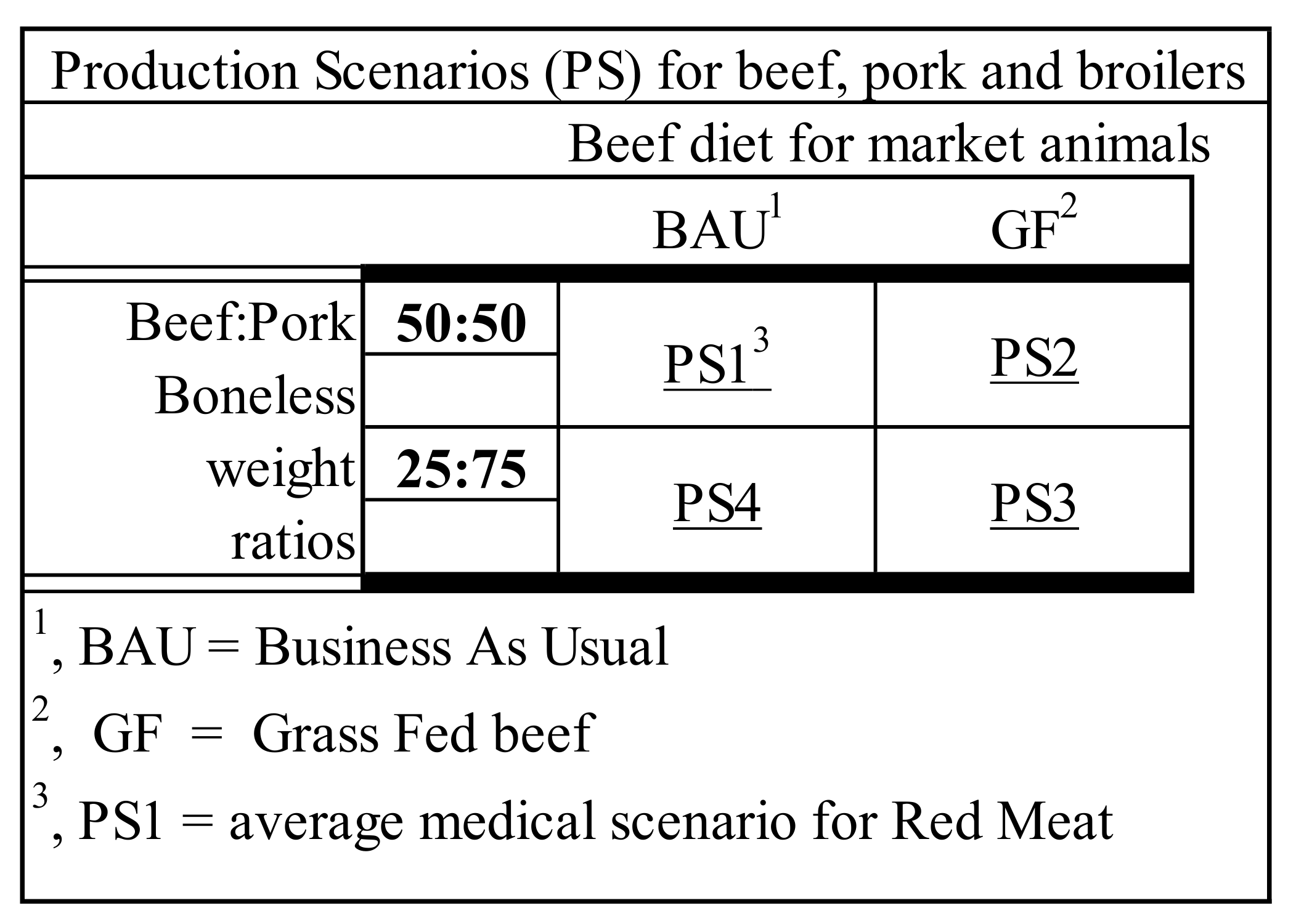
2.1.3. Livestock Production Scenarios Based on Maintaining NPI

The NPI objective function was used to generate the four production scenarios (PS) shown in Figure 2. Dyer et al. [23] created PS1, PS2 and PS3 from two beef–pork ratios and the two diet options for finishing slaughter cattle, whereas the fourth production scenario was not added until the follow up analysis [24]. Instead of three medical scenarios for reduced RM consumption, the follow up analysis used just the average medical scenario which reduced RM consumption by 25% BW. The first pair of PS (Pn(a)) assumed a 50:50 BW split between beef and pork in the RM allowed in the medical scenario, while the second pair (Pn(b)) assumed a 25:75 beef–pork BW split. The two diet options were embedded within each beef-pork pair.
The two diets for market beef cattle are represented by the two columns in Figure 2. The business as usual (BAU) diet involves no change in the most commonly used diet to finish beef for market in Canada, which is primarily the feedlot diet. Beef cattle that are prepared for market primarily on harvestable forage are referred to as grass fed (GF) beef. The BAU diet had a larger portion of feed grains than the GF diet [41,72]. Whereas statistical data were available for the BAU diet [62], the GF diet is a hypothetical system for which Dyer et al. [23] had to derive representative quantities. The two rows of Figure 2 represent the two beef:pork BW ratios. PS1 and PS2 are shown in Row 1, and PS4 and PS3 are shown in Row 2. Dyer et al. [23] defined a baseline scenario for the four PS based on the BAU beef, pork and broilers consumed by Canadians in 2017 to which the medical reduction scenario was applied. This baseline scenario for C and the four PS all shared the same protein (NPI) boundary condition (Figure 1).

2.1.4. GHG Emission Intensity Indicators

Table 2 shows the protein-based GHG emission intensities for the two methods of finishing slaughter cattle and the two non-ruminants. The protein-based intensities, Row 1, were back-calculated from output generated by Dyer et al. [23] and 2017 domestic carcass production and consumption statistics for Canada [73]. The intensities are also shown on the basis of LW in Row 2. Three of the four LW-based intensities in Row 2 were provided by Vergé et al. [41,59,60], while the fourth intensity (for GF beef) was derived by Dyer et al. [23] from unpublished output from Vergé et al. [49].
The scope of these GHG emission intensities was from field to farm gate [43]. Transport, processing and preparation were not considered. The drivers of these GHG estimates were livestock population statistics, diet and age-gender-related LW records and average crop yields [23,43,62]. GHG emissions include methane (enteric and manure), nitrous oxide (manure and commercial fertilizer) and fossil CO2 from farm inputs and fieldwork energy use, whereas soil carbon storage was not included in the emission intensities in Table 2.

2.2. Validation of Area Estimates for GF Beef

The credibility of this analysis relies on the validity of the area estimates needed for the harvestable forage that supports GF beef in Canada. Since GF beef represents assumed scenarios [23], it was not possible to collect statistical data for the area used to grow forage for this hypothetical beef production. Instead, Dyer et al. [24] interpolated these areas from data for replacement heifers generated by Vergé et al. [41,43] which had not been published prior to the RM scenario analysis [23,24]. Based on these unpublished estimates, Dyer et al. [22] showed that only about 15% of the area that supports replacement heifers in Western Canada was used to grow feed grains. Because of the big implications of the BAU-GF area differences [24,27], it was recognized that these area estimates required an independent evaluation from unrelated sources.
The parameter used for this evaluation was the feed conversion ratio (FCR), which was calculated separately for BAU and GF beef. FCR was defined by Shahbandeh [73] as the weight (kg) of feed needed to increase LW by one kg. Byrne [74] indicated that FCR should run between 4.5 and 7.5 for beef. Daily feed intake by cattle should be 4% of their body weight [54], of which they burn 50% for respiration [74]. When the product of these two feed intake guidelines were expressed on a yearly basis, they gave another estimate of FCR of 7.3. Another FCR recommendation for cattle was 8.0 [73].
The FCR from these three sources [54,73,74] were treated as independent values against which FCR estimates could be compared. The exact process by which reference FCR values were calculated was not disclosed by either Byrne [74] or Shahbandeh [73]. Therefore, two different FCR calculation processes were used, both of which were adapted to the inputs available for this analysis. The first was a grain equivalency—net LW growth and meat yield approach, while the second was a bulk feed—whole herd approach. These two FCR calculations along with the three independent FCR values [54,73,74] are shown in Figure 3.
In both processes feed supply was calculated from the products of the crop yields for feed grains and harvestable grass forage from Dyer et al. [24] shown in Table 3. To be consistent with the inputs to the scenario analysis [23], 2006 yields, were used. These yields were 2.85 and 4.10 t/ha for barley (the main feed grain used in the Canadian beef industry) and grass forage, respectively [51]. The LW that Dyer et al. [23] used for C was 1.54 Mt, based on 2017 Canadian consumption survey data [57]. The LW in Table 3 for PS1 and PS2 were also provided by Dyer et al. [23]. For PS3 and PS4 the LW was the result of reducing the beef:pork BW ratio [23,24].

2.2.1. FCR Based on Slaughter Cattle

The LW used in the first FCR calculation was equated to meat yield, or the beef cattle destined for slaughter (sc) and consumed by Canadians presented in Table 3. Additional allowance in LW growth was made for breeding cows which make up 39% of the Canadian beef population [49,72]. Half of the feed intake for beef cattle is metabolized for respiration instead of for the growth of their own bodies as replacement heifers [74]. So, to be consistent with accounting for LW growth, this LW increment for the beef cows was reduced by half. Consequently, the LW used in the first FCR calculation was increased by 20%. However, this LW increment did not change the LW of the slaughter cattle available for market.
To nullify feed quality differences, an adjustment was made for grain equivalency from the difference in the dietary energy between grass forage and feed grains. As a rule of thumb, 1.8 kg of average quality hay can replace approximately one kg of barley on the basis of nutrient energy required for cattle [51,75,76]. Using inputs of area (A) for both feed grain (g) and harvestable forage (f) for either BAU or GF beef, and the respective g and f crop yields (Y), and dividing by each of the LW for slaughter cattle (Table 3), corrected for the growth of the breeding cows, the FCRsc for both BAU and GF beef was calculated as follows.
FCRsc = (Ag × Yg + Af × Yf/1.8)/(LW × 1.2)

2.2.2. FCR Based on the Whole Herd

For the second FCR calculation, the LW shown in Table 3 were inflated from the LW of slaughter cattle to the LW of the whole herd (wh). Ignoring the calf portion of the Canadian beef cattle population, slaughter cattle accounted for 39% of the adult cattle in 2001 [41]. The feed quantities used in this FCR calculation were produced from Ag and Af converted to feed by the respective yield (Yg and Yf). Hence, the feed quality difference was ignored, and grass forage and feed grains were combined as one bulk quantity of feed in this calculation. Using the respective BAU and GF for harvestable forage and feed grains from Table 3, FCRwh was calculated for both BAU and GF beef as follows.
FCRwh = (Ag × Yg + Af × Yf)/(LW/0.39)

2.3. Assessing Area Impacts on Regenerative Grazing

The areas required for C and each PS are shown as a bar chart in Figure 4. From the perspective of climate change, the importance of regenerative grazing is its ability to sequester carbon in soils under year-round grass cover [31,34]. Given the permanency of seeded pasture, its ability to sequester additional CO2 or its risk of losing soil carbon are negligible compared to the area in harvestable forage [30,77]. Therefore, reconciling regenerative grazing with reduced RM consumption in Canada depends on how much area is devoted to harvestable forage (white bars). Due to harvestable forage being the main interest in this analysis, Figure 4 shows the feed grain areas integrated as a single quantity (black bars) for all three livestock types.

2.4. Soil Organic Carbon as a GHG Emission Offset

A decrease in soil organic carbon (∆SOC) due to perennial to annual land use change could raise agricultural GHG emissions by 2.1 tCO2/ha/year over 20 years [78]. If a change in this land use from harvestable forage to annual crops was avoided, a reduction of its carbon footprint could be credited to the beef industry [31]. Hence, the final test in this analysis was to apply this ∆SOC per ha rate to the harvestable forage area for each PS in Table 3. Figure 5 partitioned the beef GHG emissions in Table 3 into a portion that could be nullified by ∆SOC (gray) and net beef GHG emissions (white), or the residuals from the GHG emissions shown in Table 3. Figure 5 also compares the GHG emitted by beef with the GHG emissions from pork production (black). For this test the LW of pork was assumed to equal the LW of the beef in Table 3, converted to GHG emissions using the pork GHG/LW coefficient from Table 2.

3. Results

3.1. FCR Estimates for Validating Areas for GF Beef

The land areas shown in the first two columns of Table 3 were provided by Dyer et al. [24]. For the BAU scenarios (C, PS1 and PS4) the harvestable forage areas were three times the feed grain areas that support beef production. For the two GF scenarios (PS2 and PS3) the harvestable forage areas were 10.6 times the feed grain areas for beef. These ratios suggest that GF beef production uses 3.5 times as much area in harvestable forage as BAU beef production, relative to their respective feed grain areas. The land used for seeded pasture was excluded because this land use was not interchangeable with growing feed grains [77]. These FCR comparisons were not affected by this exclusion because this land use mainly supports the breeding cows which were assumed to be the same for both the BAU and GF beef production systems. Converting the areas to feed production raised the two harvestable forages to feed grain ratios (Columns 3 and 4) to 4.4 and 15.3 for the BAU and GF scenarios, respectively, due to the differences in yield.
In Figure 3, the GF beef estimate from FCRwh was 11% lower than the FCR derived from NRCS-USDA [54] (FCR-2), whereas the estimate by FCRsc for GF beef was 12% higher than FCR-2, but exceeded the FCR from Shahbandeh, [73] (FCR-3) by only 2%. FCR-3 exceeded the FCRwh estimate for GF beef by 19%. For BAU beef, FCRsc exceeded the lower FCR value from Byrne [74] (FCR-1) by 21%, whereas the lower FCR-1 value exceeded the GF estimate from FCRwh by 12%.
The FRC averages from Equations (1) and (2) (Table 3) generated only two unique FCR values for all PS and C, which are shown by two right-pointing arrows in Figure 3. The top arrow, which shows the average GF estimate (white sections), intersects FCR-1 just below the higher FCR from Byrne [74], while the bottom arrow, which shows the average BAU estimate (black sections), intersects FCR-1 just above the lower Byrne [74] FCR. At 7.3, the FCRsc and FCRwh average for GF beef equaled the NRCS-USDA [54] FCR and was comfortably below the FCR from Shahbandeh [73] and was just barely below the highest FCR from Byrne [74]. At 4.7, the average FCR for BAU beef was only 5% above the lower FCR from Byrne [74].
The range in FCR from Byrne [74] (FRC-1) provided the most useful comparison. FCRsc and FCRwh both had similar and overlapping ranges with FRC-1 (Figure 3). The high side of the range reported by Byrne [74] exceeded the low side from Byrne [74] by 67%. For FRCsc (Equation (1)), the GF estimate exceeded the BAU estimate by only 49%. The GF to BAU difference given by FCRwh (Equation (2)), was 63%, for an average GF to BAU difference of 55%. Hence, the combined GF to BAU range from the FCRsc and FCRwh was less than the FCR range (FCR-1) reported by Byrne [74].

3.2. GHG-Protein Ratios for GF Beef

Even though the range of GHG to protein ratios for beef from Nijdam et al. [65] were too wide for quantitative verification, they provided a relative comparison. Much of this range can be explained by which country produced the beef [42]. The 20% difference between the BAU and GF beef GHG–protein ratios in Line 1 of Table 2 reflects the 20% difference between intensive and extensive beef systems shown by Nijdam et al. [65]. The magnitudes by which the beef GHG–protein ratios exceed the GHG-protein ratios for pigs and poultry in the Nijdam et al. [65] analysis, and pork and chicken in the de Vries and de Boer [63] analysis, both showed similar magnitudes by which both the beef GHG to protein ratios in Table 2 exceeded the GHG–protein ratios for pork and broilers.
When the LW for PS1, PS2 and PS3 in Table 3 are multiplied by the LW based GHG emission intensities for BAU and GF beef from Table 2 (Row 2) the results equal the GHG emissions shown by Dyer et al. [23] for these three PS. With the LW for PS3 and PS4 being half the LW for PS2 and PS1, respectively, the derivation of the GHG emissions from beef for PS4 from Table 1 and Table 2 also agree with the beef GHG emissions for PS4 reported by Dyer et al. [24]. These GHG estimates are shown in Column 7 of Table 3.

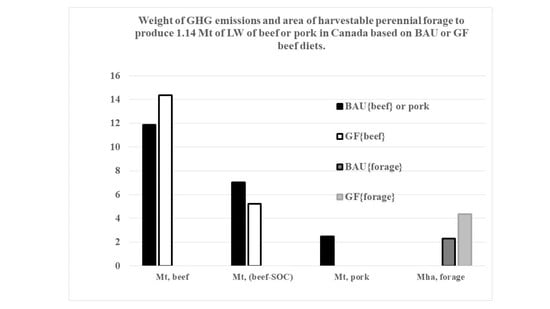
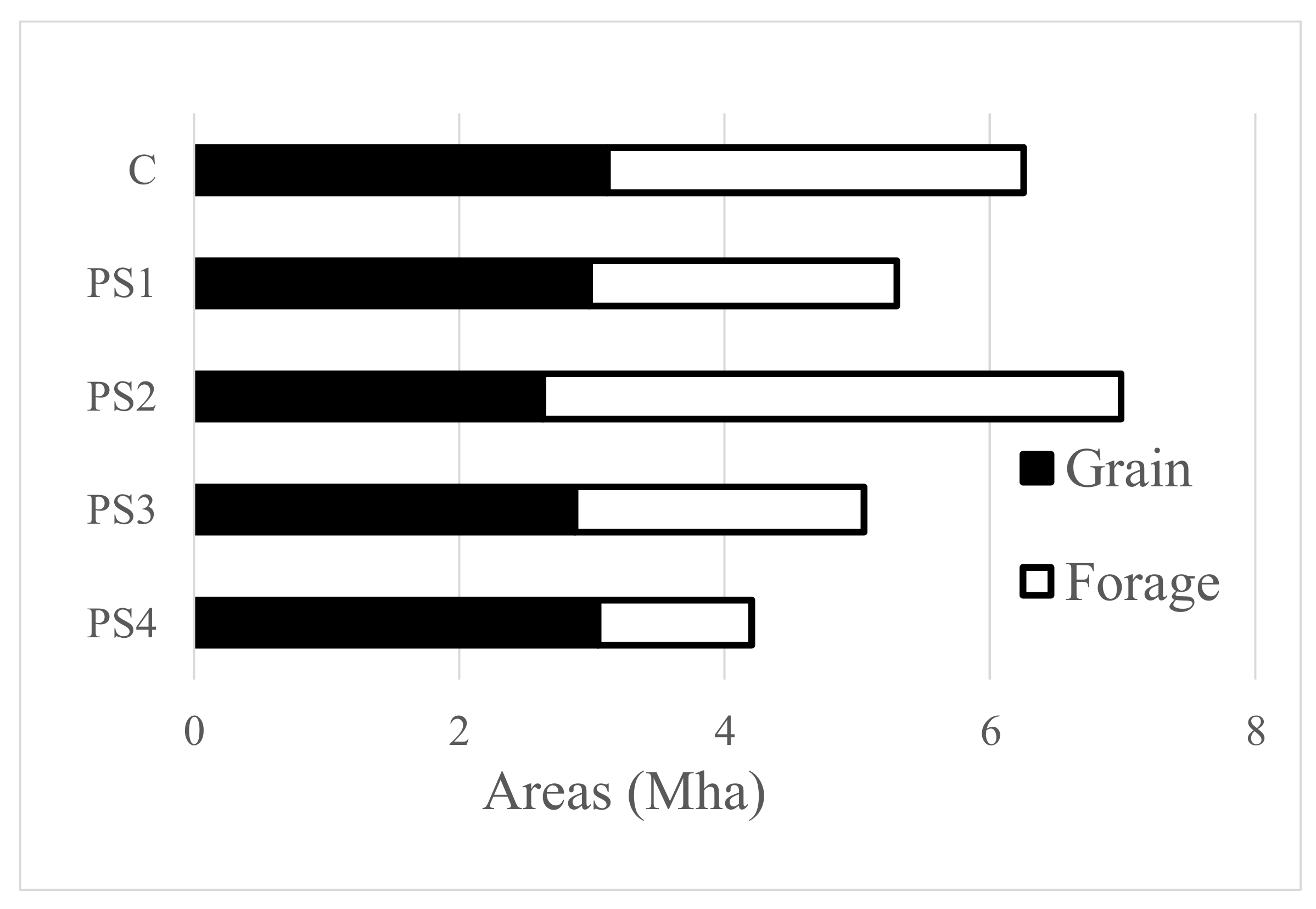
3.3. Harvestable Forage Area Changes among Scenarios

Due to the grain areas in Figure 4 (black bars) containing the feed needed for the two non-ruminants, as well as beef, these grain areas are both less variable across the PS and are a larger portion of the total crop areas in each PS than are the grain areas in Table 3. While the range in feed grain areas among PS1, PS3 and PS4 in Figure 4 was only 6% of their average area, the feed grain for PS2 was 11% below this average. PS2 required 1.7 Mha more land in total than PS1 and 1.9 Mha more than PS3 (Figure 4), which represent 32% and 38% margins in total land use by PS2 over PS1 and PS3, respectively.
Figure 4 showed greater variation among the harvestable forage areas (white bars) than among the feed grain areas. The harvestable forage areas for GF beef (PS2 and PS3) received special attention in this analysis. PS2 used 40% more land for harvestable forage production than was used by C, even though PS2 produced 26% less LW beef than C (Table 3). PS2 had twice as much land in harvestable forage as PS3 and 1.9 times as much land in harvestable forage as PS1. PS3 used almost twice as much harvestable forage as PS4, but slightly less harvestable forage area than PS1. Compared to C, PS3 used almost as much area (92%) for feed grain, but almost a third (31%) less harvestable forage area.

3.4. The Role of Seeded Pasture

With the reduction of the beef crop complex areas to just the areas that supported Canadian-consumed beef, and after projecting forward from 2001 to 2017, as was done by Dyer et al. [23,24], seeded pasture accounted for 2.2 Mha in C, instead of 4.3 Mha. With the same scaling down from C to the four PS, it could have some impact on the interpretation of Figure 4. For PS1 and PS2 seeded pasture would drop to 1.6 Mha. Since the area in seeded pasture (natural grassland excluded) is defined by the needs of the beef breeding herd, it will not be affected by the BAU-GF diet difference (columns of Figure 2) which only applies to the slaughter cattle. However, this need for seeded pasture would be reduced to half by the change in the beef:pork ratio (rows of Figure 2). Hence, seeded pasture would drop to 0.8 Mha for PS3 and PS4.
If the scaled down seeded pasture areas were added to C and the four PS in Figure 4, the gaps between PS2 and both PS3 and PS4 would widen, while for PS2 and C the gap would narrow. The gaps between C and both PS3 and PS4 would also widen. However, it can be argued that, because seeded pasture areas were not interchangeable with annual crops in this analysis, and because C and the four PS all produced the same amount of protein, the seeded pasture area required for C would also be available to all four PS and would therefore have no direct impact on the differences shown in Figure 4.

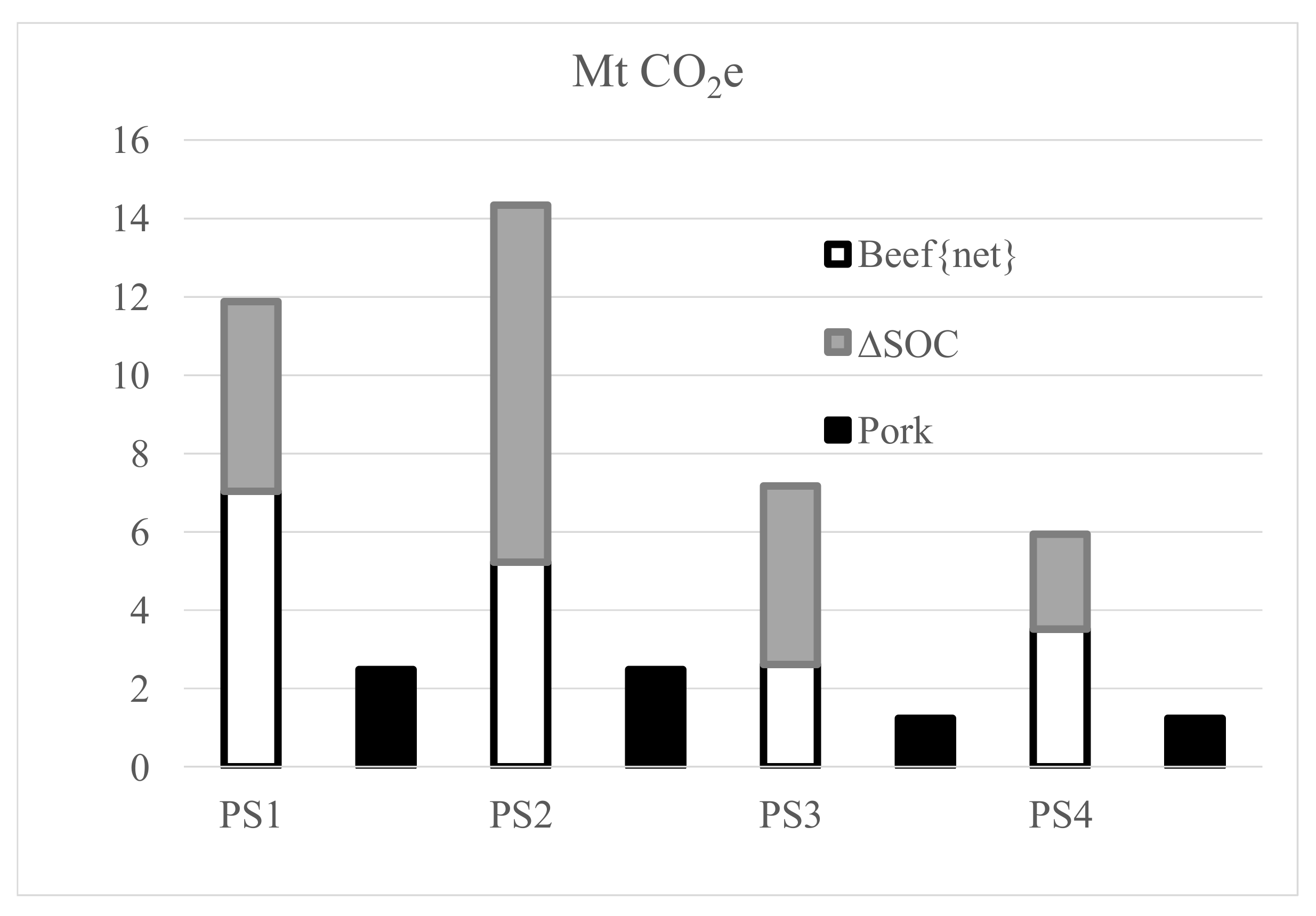
3.5. Soil Organic Carbon under Harvestable Forage

In Figure 5 the two beef scenarios with the greatest proportional offset by ∆SOC were PS2 and PS3, for which the net beef GHG emissions were reduced from almost six times to just twice the respective GHG emissions from pork production. For PS1 and PS4 net beef GHG emissions were still almost three times the pork GHG emissions, down from just less than five times pork. Hence, ∆SOC did not offset enough ruminant methane emissions to justify GF beef as a protein source compared to pork. However, the ∆SOC changed the GHG-based ranking of the four PS. PS1 replaced PS2 as the highest GHG emissions after the ∆SOC offset, whereas PS3 replaced PS4 as the lowest. The largest ∆SOC offset was to PS2, while the smallest was to PS4.

4. Discussion

The findings of this analysis resulted from a mix of methodologies. Much of it entailed meta-analysis as it relied heavily on seeking a consensus on regenerative agriculture and on previous carbon foot printing of Canadian livestock. It would be inaccurate to describe this early Canadian work as LCA, even though it employed many LCA processes, because it did not account for impacts outside the farm gate. While the use of RM and NPI boundary conditions in Figure 1 suggest a simplified form of linear programming, this phase of the analysis was also a meta-analysis, since the results from the algorithm in Figure 1 were drawn from two previous papers [23,24]. However, as illustrated in Figure 2, these two papers are best described simply as scenario analysis. The last three stages of the analysis interpreted the land use changes associated with the four scenarios. These stages included verifying the GF forage areas through FCR (Figure 3), area-based PS comparisons (Figure 4) and expressing harvestable forage areas as avoided GHG emissions (Figure 5), can only be described as quantitative scenario analysis. Since these are the stages specific to this analysis, scenario analysis is the best way to describe this methodology.

4.1. FCR as a Performance Measure for Harvestable Forage Areas

For the average of the two FCR estimates for BAU beef (4.7) to be so close to the lower FCR value from Byrne [74] is a source of confidence in the combined FRC estimates from Equations (1) and (2), but not surprising since the area and yield inputs for the BAU estimates were derived from actual statistical data. As well, neither of the BAU estimates were very different than the lowest FCR from Byrne [74]. Since the crop areas for both GF scenarios were interpolated from unpublished simulation results [43], this agreement suggests that at least the average of the two FCR calculations for GF beef (7.3) was also valid.
More important was that the BAU to GF ranges of the FCR estimates and their averages in Figure 3 were all slightly less than the range reported by Byrne [74]. Several factors contribute to GF and BAU differences in FCR. The first is the lower LW productivity to be expected from GF beef than BAU beef [36]. GF slaughter cattle often have less shelter from extreme temperature stresses [45,47], consume lower energy feed [62] and live longer [39,79] than feedlot cattle, and walk and respire more during their lives. The productivity of the beef feedlot industry in Canada is also inflated by the culled dairy calves sent to feedlots [43], for which their pre-feedlot life cycle stages are charged to the dairy industry [41,72]. Since these effects appear to have been captured by the BAU-GF differences in FCR in Figure 3, without over-estimating the FCR range [74], the BAU-GF differences in areas in Figure 4 also appear to be valid. The FCR comparisons in Figure 3 (along with the explainable differences) made a credible case that the GF harvestable forage area estimates (Figure 4) that underpinned the two GF-based PS were valid.

4.2. Reliability of the Area and GHG Emission Estimates for GF Beef

Since the FCR estimates for BAU and GF beef used the same LW, the areas for harvestable forage (Table 3) used in the scenario analysis [23,24] were acceptably accurate and were reassuring for achieving the goals of this analysis. However, an independent source was not available for validating the GHG emissions from the GF beef. However, it is widely acknowledged that GF beef will emit more GHG, mainly enteric methane than the same LW of beef raised in feedlots [45,46,47,80] and that cattle diets determine the intensity of the enteric methane emissions [81,82]. Additionally, the GHG–protein ratios for extensive to intensive beef production systems from de Vries and de Boer [63] and Nijdam et al. [65] supports the difference between the GHG emissions estimates for BAU and GF beef reported in this analysis.

4.3. Impact of Harvestable Forage for GF Beef on Land Use

When the PS were ranked by their GHG emissions (Table 3), PS2 was the highest, while PS3 was the second lowest of the four scenarios. Not only is PS2 a greater source of GHG emissions, it requires much more cropland to grow harvestable forage than do the other three PS. Figure 4 demonstrates that, as concluded by Dyer et al. [24], the difference in soil carbon sequestration potentially associated with PS2 cannot be charged against the other three scenarios simply because that land was not required in those three scenarios, and could have been returned to natural habitat. Additionally, if the 1.7 Mha of surplus land in PS2 over PS1 (Figure 4) was previously natural grassland, converting it to either improved grazing land or hay, with a stated aim of sequestering carbon, would be contrary to the Project Drawdown [11] guidance. Over dependence on harvestable forage, such as in PS2, could also necessitate harvesting hay from seeded pasture, which could lead to both seeded pasture and some rangeland being over grazed by the breeding cows.
PS3, on the other hand, required slightly less land to be brought under harvestable forage, and less total cropland, than PS1, as well as emitting less GHG than either PS1 or PS2. While PS3 used more land and emitted more GHG than PS4, it could facilitate the benefits of regenerative grazing that PS4 would fail to provide. From these scenarios it does not appear to make sense to either maintain or expand beef production while also converting grain-fed beef to grass-fed beef (as in PS2), even when soil carbon is considered. However, converting more land to GF beef may be sustainable if this conversion is linked with a lower per ha expectation for protein production from GF beef [36], as in PS3.
In contrast, it cannot be overlooked that PS4 releases land from harvestable forage. Ideally this land could be retired from agricultural use, thus invoking all the ecological benefits of natural habitat [11]. This land could be left as harvestable forage or pasture, resulting in yet more beef production, which would essentially turn a PS4 into a scenario much more like PS3. Seeding this land to annual crops, the option that the avoided ΔSOC strategy is meant to prevent [31], could have several feedback impacts. If the crops seeded are feed grains, the ruminant/non-ruminant balance would shift towards the latter. This would lower the carbon footprint of the Canadian livestock industry, but could compromise the move towards less RM [23], depending on how much of the feed grains were fed to pork instead of broilers. Seeding to crops for human consumption could alleviate pressure on world food supply [1,4] if the produce was made available to international famine relief agencies. In that role, it could, arguably, displace the need to cultivate land that is less suitable for grain crops elsewhere in the world. Alternatively, if the annual crop produced a commodity not essential to human survival, it is equally arguable that the land freed under PS4 would represent a lost opportunity to reduce the carbon footprint of agriculture even more than what was possible under PS4. However, the speculative nature of all of these options illustrates the merits of the closed system model described in Figure 1 and Figure 2.

4.4. Implications of the Protein Boundary Condition for the PS Analysis

In Figure 4, PS3 and PS4 used less land for both grains and harvestable forages than both PS1 and PS2 because of the greater efficiency of the two non-ruminants compared to beef cattle, which is consistent with the differences in FCR (Figure 3) and the lower reproductive efficiency of beef cattle [18]. These land use differences could not have been quantified without the boundary condition form of the GHG-protein indicator. In setting protein supply as an objective function (boundary condition), this carcass producing industry became the closed system described in Figure 1. Hence, these findings are theoretical because the actual on-farm livestock production decisions would be driven by market preferences, rather than from optimizing access to protein in the Canadian food basket.
The protein boundary condition also made the comparison of all the area totals in Figure 4 possible, because all of these areas equated to the same protein quantity. Thus, Figure 4 was implicitly an area-protein indicator with greater importance than the GHG-protein indicator for this analysis. By asking the question of how much animal carcass do we need in our food basket, these two indicators have the potential to change the debate on the role of livestock production in the human food chain of the 21st century. Focusing on just these two indicators as the only two metrics for this analysis, however, must not overshadow the non-climate related environmental benefits and potential impacts by regenerative grazing.
Because the areas shown in Figure 4 were derived from Canadian protein consumption data, rather than total livestock production statistics, they appear small in comparison to the land base that supports the entire Canadian beef industry [31,41]. However, this scenario analysis can still provide useful insight for the entire Canadian livestock industry if Figure 4 is treated as a sample of that industry.

4.5. Impact of Soil Organic Carbon

With all four net beef GHG emissions well above the respective pork GHG emissions (Figure 5), the test for ∆SOC clearly demonstrated that ∆SOC cannot out-weigh the advantage of pork over beef for combatting climate change. In addition, the very generous allowance in this test for avoided GHG emissions represents the most optimistic case for GF beef as a tool to combat climate change. Firstly, this test was based solely on pork, for which the protein per GHG emission intensity is 2.3 times as high as that for broilers [18], whereas Dyer et al. [23] used a combination of these two commodities to represent non-ruminants. Hence all of the net beef to pork ratios reported for Figure 5 would be much greater if pork were replaced by a mix of the two non-ruminants.
This allowance also ignored that the land credited with ∆SOC avoidance in PS2 exceeded the harvestable forage land in PS1 by 89% and in C by 39%, which brings additional land into the closed land use system described in Figure 1. In addition, when beef consumption was cut in half in PS3 and PS4, feed grain areas (Figure 4) showed no increase compared to either C or PS1. This suggests that, at least for the closed system defined by this scenario analysis, there was no conversion of area in perennial forage to annual feed grain, and no ∆SOC to be avoided, which reflects the inefficiency of cattle, compared to non-ruminants as a protein source. However, showing that the two GF scenarios (PS2 and PS3) received the most reduction from the hypothetical ∆SOC demonstrated that maintaining perennial crops to mitigate climate change [31] was more feasible for GF than BAU beef.

4.6. Limitations of the Study

There are several limitations about this study to be noted. The first was that the system boundary of the GHG emission intensities was the farm gate. The second was that it treated Canada as one geographic region, whereas Canadian livestock are dispersed over many distinct climatic and geographic regions. The third limitation was that the GHG emission intensities in Table 2 were derived from 2001 and projected forward to 2017, during which time livestock production methods have evolved. The fourth limitation stems from the model in Figure 1 being a closed system. For example, limiting beef consumption and choosing GF beef might not limit the industry’s activity. These consumer responses may cause producers to turn to more exports. In reality, however, producers can always be expected to maximize exports, regardless of domestic consumption because Canada has no quota on beef production. So, exports may not be very sensitive to domestic consumption. In addition, increasing the supply of beef on the international market could actually suppress production in other countries where, in some cases, the land base is much more vulnerable to free roaming cattle.

5. Conclusions

This paper added value to the understanding of Canada’s carcass production industries and reduced a complex and contradictory set of choices to a two-by-two decision process (Figure 2). The results from this study should provide a way forward for reconciling regenerative grazing (as defined in this study) with reducing livestock GHG emissions in Canada. The optimum beef management strategy for this reconciliation appears to be to reduce the share of beef in the Canadian food basket along with the modest remaining share allotted to beef being GF beef.
Whereas Dyer et al. [24] concluded that PS4 was the optimum protein production scenario for Canada, this analysis recognized that PS3 reduced GHG emissions without significantly increasing harvestable forage areas. The possibility that PS3 could have the lowest GHG emissions after the ∆SOC offset (Figure 5) added weight to PS3 being a better option for reconciling with regenerative agriculture than PS4. This approach treats GF beef, not just as a protein source, but also as a tool for restoring and protecting the agricultural land base, while offering some economic payback to the beef producers. However, Figure 5 did not overturn the conclusion that non-ruminants are more compatible with reducing climate change than beef, even with the generous allowance for avoided ∆SOC under harvestable forage. Implicit in this reconciliation is that, while allowing more GHG emissions to achieve greater carcass production is not sustainable, a limited increase in GHG emissions (over PS4) for the sake of all the benefits credited to regenerative grazing could be an acceptable trade-off, depending on the geographic setting.
In favoring PS4, Dyer et al. [24] provided clear options for consumers to influence the agricultural carbon footprint: consume less RM and favor non-ruminant over ruminant protein sources. Whether the consumer has a role in reconciling regenerative grazing with reduced GHG emissions is not so clear. Choosing non-ruminants over ruminants and reducing RM consumption would still be effective (for example in avoiding PS2), but how do consumers collectively achieve PS3? Simplistically, buying more pork and broilers instead of beef can be coupled with only buying GF beef as an occasional alternative. One answer may be to buy local when shopping for beef to allow shoppers to better judge for themselves the desired conditions of production, such as that it must actually be GF beef. For those living in a high-rise in the center of a big city, however, this option may not always be available.
But for assessing whether the regenerative grazing concept is being used primarily as a tool to restore the land, stocking rates must be sustainably low [49] and beef should not be the only produce and income source from that farm. Beef farmers have to be partners in this shift in consumer habits. Rather than trying to charge a premium for their produce, they need to embrace ruminants as the only way to turn grass into protein [44], that the lower production costs of farming grass instead of annual crops will at least partly compensate for the lower productivity of GF beef [36] and that improved soil performance stemming from regenerative grazing [34] may lead to a more stable farm income in the long term. Barring these criteria being met, PS4 is still the best fall back choice for consumers.

Author Contributions

Conceptualization, J.A.D. and R.L.D.; methodology, J.A.D.; formal analysis, J.A.D.; resources, R.L.D.; writing—original draft preparation, J.A.D.; writing—review and editing, R.L.D. Desjardins; funding acquisition, R.L.D. All authors have read and agreed to the published version of the manuscript.

Funding

This research was funded by the Sustainability Metrics Project, Contract No. 01E86 2018–2019, Agriculture and Agri-food Canada, Government of Canada.

Institutional Review Board Statement

Not applicable.

Informed Consent Statement

Not applicable.

Data Availability Statement

Data sharing not applicable.

Acknowledgments

The authors wish to acknowledge Darrel D. Cerkowniak, Senior Science Data Analyst, Agrienvironment Division, AAFC, Saskatoon, Saskatchewan, for guidance in interpreting the potential soil organic carbon change for changing from perennial to annual livestock feed production as a Canada-wide coefficient.

Conflicts of Interest

The authors declare no conflict of interest.

References

  1. Food and Agriculture Organization of the United Nations. Climate Change and Food Security: A Framework Document. 2008. Available online: www.fao.org/3/k2595e/k2595e00.htm. (accessed on 15 April 2021).
  2. Henchion, M.; Hayes, M.; Mullen, A.M.; Fenelon, M.; Tiwari, B. Future Protein Supply and Demand: Strategies and Factors Influencing a Sustainable Equilibrium. Foods 2017, 6, 53. [Google Scholar] [CrossRef] [PubMed] [Green Version]
  3. Mussell, A.; Bilyea, T.; Zafiriou, M. Efficient Agriculture as a Greenhouse Gas Solutions Provider. The Canadian Agri-Food Policy Institute. 2019. Available online: https://capi-icpa.ca/explore/resources/efficient-agriculture-as-a-greenhouse-gas-solutions-provider/. (accessed on 5 April 2021).
  4. Bakkegaard, R.K.; Møller, L.R.; Bakhtiari, F. Joint Adaptation and Mitigation in Agriculture and Forestry; Working Paper; UNEP DTU: Copenhagen, Denmark, 2016; p. 36. [Google Scholar] [CrossRef]
  5. Almiron, N. Meat taboo: Climate Change and the EU Meat Lobby. In Meatsplaining, The Animal Industry and the Rhetoric of Denial; Hannan, J., Ed.; Sydney University Press: Sydney, Australia, 2020; ISBN 9781743327104. [Google Scholar]
  6. Cui, Y.; Khan, S.U.; Deng, Y.; Zhao, M. Regional difference decomposition and its spatiotemporal dynamic evolution of Chinese agricultural carbon emission: Considering carbon sink effect. Environ. Sci. Pollut. Res. 2021, 1–20. [Google Scholar] [CrossRef]
  7. Teague, W.R.; Apfelbaum, S.; Lal, R.; Kreuter, U.P.; Rowntree, J.; Davies, C.A.; Conser, R.; Rasmussen, M.; Hatfield, J.; Wang, T.; et al. The role of ruminants in reducing agriculture’s carbon footprint in North America. J. Soil Water Conserv. 2016, 71, 156–164. [Google Scholar] [CrossRef] [Green Version]
  8. Yohannes, J. A Review on Relationship between Climate Change and Agriculture. J. Earth Sci. Clim. Chang. 2016, 7, 1–8. [Google Scholar] [CrossRef]
  9. Carrington, D. Giving Up Beef Will Reduce Carbon Footprint More Than Cars. The Guardian. 2014. Available online: www.theguardian.com/environment/2014/jul/21/giving-up-beef-reduce-carbon-footprint-more-than-cars (accessed on 1 March 2021).
  10. Majot, J.; Kuyek, D. Big Meat and Big Dairy’s Climate Emissions put Exxon Mobil to Shame. The Guardian. 2017. Available online: www.theguardian.com/commentisfree/2017/nov/07/big-meat-big-dairy-carbon-emmissions-exxon-mobil. (accessed on 1 March 2021).
  11. Project Drawdown. Farming Our Way Out of the Climate Crisis. 2017. Available online: https://globalecoguy.org/farming-our-way-out-of-the-climate-crisis-c235e1aaff8d (accessed on 4 March 2021).
  12. Delgado, J.A.; Groffman, P.M.; Nearing, M.A.; Goddard, T.; Reicosky, D.; Lal, R.; Kitchen, N.R.; Rice, C.W.; Towery, D.; Salon, P. Conservation practices to mitigate and adapt to climate change. J. Soil Water Conserv. 2011, 66, 118A–129A. [Google Scholar] [CrossRef] [Green Version]
  13. Smith, P.; Calvin, K.; Nkem, J.; Campbell, D.; Cherubini, F.; Grassi, G.; Korotkov, V.; Le Hoang, A.; Lwasa, S.; McElwee, P.; et al. Which practices co-deliver food security, climate change mitigation and adaptation, and combat land degradation and desertification? Glob. Chang. Biol. 2020, 3, 1532–1575. [Google Scholar] [CrossRef] [Green Version]
  14. Hood, M. G20 Carbon ‘Food-Print’ Highest in Meat-Loving Nations: Report. 2020. Available online: https://phys.org/news/2020-07-g20-carbon-food-print-highest-meat-loving.html? (accessed on 13 February 2021).
  15. Nardone, A.; Ronchi, B.; Lacetera, N.; Ranieri, M.S.; Bernabucci, U. Effects of climate changes on animal production and sustainability of livestock systems. Livest. Sci. 2010, 130, 57–69. [Google Scholar] [CrossRef]
  16. O’Mara, F.P.; Beauchemin, K.A.; Kreuzer, M.; McAllister, T.A. Reduction of Greenhouse Gas Emissions of Ruminants Through Nutritional Strategies. In Proceedings of the International Conference Livestock and Global Climate Change, Hammamet, Tunisia, 17–20 May 2008; Rowlinson, P., Steele, M., Nefzaoui, A., Eds.; British Society of Animal Science: Midlothian, UK, 2008. Available online: www.bsas.org.uk (accessed on 10 July 2021).
  17. Morgan, C.B. I eat, therefore I’m evil: The dilemmas of applying climate justice to food choice. In Local Action for Global Climate Justice. The Great Lakes Watershed; Perkins, P.E., Ed.; Routledge: New York, NY, USA, 2020; pp. 131–144. ISBN 978-0-429-32070-5. [Google Scholar]
  18. Dyer, J.A.; Vergé, X.P.C.; Desjardins, R.L.; Worth, D.E. The protein-based GHG emission intensity for livestock products in Canada. J. Sustain. Agric. 2010, 34, 618–629. [Google Scholar] [CrossRef]
  19. Cusack, D.F.; Kazanski, C.E.; Hedgpeth, A.; Chow, K.; Cordeiro, A.L.; Karpman, J.; Ryals, R. Reducing climate impacts of beef production: A synthesis of life cycle assessments across management systems and global regions. Glob. Chang. Biol. 2021, 27, 1721–1736. [Google Scholar] [CrossRef]
  20. Ripple, W.J.; Smith, P.; Haberl, H.; Montzka, S.A.; McAlpine, C.; Boucher, D.H. Ruminants, climate change and climate policy. Nat. Clim. Chang. 2014, 4, 2–5. [Google Scholar] [CrossRef]
  21. Truth or Drought. Myth: Livestock Grazing, When Done Right, is Beneficial and Necessary. 2020. Available online: www.truthordrought.com/holistic-grazing-myths (accessed on 29 March 2021).
  22. Dyer, J.A.; Vergé, X.P.C.; Desjardins, R.L.; McConkey, B.G. Implications of biofuel feedstock crops for the livestock feed industry in Canada. In Environmental Impact of Biofuels; Dos Santos, B.M.A., Ed.; InTech Open Access Publisher: Rijeka, Croatia, 2011; pp. 161–178. ISBN 978-953-307-479-5. [Google Scholar]
  23. Dyer, J.A.; Worth, D.E.; Vergé, X.P.C.; Desjardins, R.L. Impact of recommended red meat consumption in Canada on the carbon footprint of Canadian livestock production. J. Clean. Prod. 2020, 266, 121785. [Google Scholar] [CrossRef]
  24. Dyer, J.A.; Desjardins, R.L.; Worth, D.E.; Vergé, X.P.C. Potential Role for Consumers to Reduce Canadian Agricultural GHG Emissions by Diversifying Animal Protein Sources. Sustainability 2020, 12, 5466. [Google Scholar] [CrossRef]
  25. Mandal, A. Red and Processed Meats—How Much to Include in Diets? Medical Research News. 2011. Available online: www.news-medical.net/news/20110222/Red-and-processed-meats-How-much-to-include-in-diet.aspx (accessed on 15 March 2021).
  26. Dyer, J.A.; Vergé, X.P.C.; Kulshreshtha, S.N.; Desjardins, R.L.; McConkey, B.G. Areas and greenhouse gas emissions from feed crops not used in Canadian livestock production in 2001. J. Sustain. Agric. 2011, 35, 780–803. [Google Scholar] [CrossRef]
  27. Dyer, J.; Desjardins, R. Protein as a Unifying metric for carbon footprinting livestock. Res. Outreach Publ. Earth Environ. 2020, 118, 142–145. Available online: https://researchoutreach.org/wp-content/uploads/2020/10/James-Dyer-and-Raymond-Desjardins.pdf (accessed on 1 April 2021).
  28. Veeramani, A. Carbon Footprinting Dietary Choices in Ontario: A Life Cycle Approach to Assessing Sustainable, Healthy & Socially Acceptable Diets. Master’s Thesis, Waterloo University, Waterloo, ON, Canada, 2015; p. 173. [Google Scholar]
  29. Patle, G.T.; Badyopadhyay, K.K.; Kumar, M. An overview of organic agriculture: A potential strategy for climate change mitigation. J. Appl. Nat. Sci. 2014, 6, 872–879. [Google Scholar] [CrossRef] [Green Version]
  30. Boehm, M.; Junkins, B.; Desjardins, R.L.; Kulshreshtha, S.; Lindwall, W. Sink potential of Canadian agricultural soils. Clim. Change 2004, 65, 297–314. [Google Scholar] [CrossRef]
  31. Liang, C.; MacDonald, J.D.; Desjardins, R.L.; McConkey, B.G.; Beauchemin, K.A.; Flemming, C.; Cerkowniak, D.; Blondel, A. Beef cattle production impacts soil carbon storage. Sci. Total Environ. 2020, 718, 137273. [Google Scholar] [CrossRef]
  32. EIT Food. Can Regenerative Agriculture Replace Conventional Farming? European Institute of Innovation & Technology (EIT). 2020. Available online: www.eitfood.eu/blog/post/can-regenerative-agriculture-replace-conventional-farming (accessed on 4 March 2021).
  33. Elliot, R. A Close Look at Regenerative Agriculture in Ontario. Ontario Culinary. 2020. Available online: https://ontarioculinary.com/a-close-look-at-regenerative-agriculture-in-ontario/ (accessed on 13 February 2021).
  34. Hoeffner, K.; Beylich, A.; Chabbi, A.; Cluzeau, D.; Dascalu, D.; Graefe, U.; Guzmán, G.; Hallaire, V.; Hanisch, J.; Landa, B.B.; et al. Legacy effects of temporary grassland in annual crop rotation on soil ecosystem services. Sci. Total. Environ. 2021, 780, 146140. [Google Scholar] [CrossRef]
  35. Liebig, M.A.; Gross, J.R.; Kronberg, S.L.; Phillips, R.L. Grazing Management Contributions to Net Global Warming Potential: A Long-term Evaluation in the Northern Great Plains. J. Environ. Qual. 2010, 39, 799–809. [Google Scholar] [CrossRef]
  36. Kenyon, S. What is Regenerative Grazing? From the Ground Up. Canadian Cattlemen. 2020. Available online: https://www.canadiancattlemen.ca/from-the-ground-up/what-is-regenerative-grazing/ (accessed on 13 February 2021).
  37. NSAC. Agriculture and Climate Change: Policy Imperatives and Opportunities to Help Producers Meet the Challenge; National Sustainable Agriculture Coalition: Washington, DC, USA, 2019; Available online: https://sustainableagriculture.net (accessed on 10 July 2021).
  38. Searchinger, T.; Heimlich, R.; Houghton, R.A.; Dong, F.; Elobeid, A.; Fabiosa, J.; Tokgoz, S.; Hayes, D.; Yu, T.-H. Use of U.S. croplands for biofuels increases greenhouse gases through emissions from land use change. Science 2008, 319, 1238–1240. [Google Scholar] [CrossRef]
  39. Matsumoto, N. Is Grass-Fed Beef Really Better For The Planet? Here’s The Science. NPR. 2019. Available online: www.npr.org/sections/thesalt/2019/08/13/746576239/is-grass-fed-beef-really-better-for-the-planet-heres-the-science (accessed on 11 February 2021).
  40. Ma, Z.; Shrestha, B.M.; Bork, E.W.; Chang, S.X.; Carlyle, C.N.; Döbert, T.F.; Silva Sobrinho, L.; Boyce, M.S. Soil greenhouse gas emissions and grazing management in northern temperate grasslandsSci. Total Environ.2021; Volume 796, p. 148975. [CrossRef]
  41. Vergé, X.P.; Dyer, J.A.; Desjardins, R.L.; Worth, D.E. Greenhouse gas emissions from the Canadian beef industry. Agric. Syst. 2008, 98, 126–134. [Google Scholar] [CrossRef]
  42. Desjardins, R.L.; Worth, D.E.; Vergé, X.P.C.; Maxime, D.; Dyer, J.; Cerkowniak, D. Carbon Footprint of Beef Cattle. Sustainability 2012, 4, 3279–3301. [Google Scholar] [CrossRef] [Green Version]
  43. Vergé, X.P.; Dyer, J.A.; Worth, D.E.; Smith, W.N.; Desjardins, R.L.; McConkey, B.G. A Greenhouse Gas and Soil Carbon Model for Estimating the Carbon Footprint of Livestock Production in Canada. Animals 2012, 2, 437–454. [Google Scholar] [CrossRef] [PubMed]
  44. Chauhan, D.S.; Ghosh, N. Impact of Climate Change on Livestock Production: A Review. J. Anim. Res. 2014, 4, 223. [Google Scholar] [CrossRef]
  45. Mangino, J.; Peterson, K.; Jacobs, H. Development of an Emissions Model to Estimate Methane from Enteric Fermentation in Cattle. U.S. Environmental Protection Agency. 2003. Available online: https://www.researchgate.net/publication/228465202 (accessed on 16 March 2021).
  46. Sejian, V.; Samal, L.; Haque, N.; Bagath, M.; Hyder, I.; Maurya, V.P.; Bhatta, R.; Ravindra, J.P.; Prasad, C.S.; Lal, R. Overview on adaptation, mitigation and amelioration strategies to improve livestock production under the changing climatic scenario. In Climate Change Impact on Livestock: Adaptation and Mitigation; Sejian, V., Gaughan, J., Baumgard, L., Prasad, C., Eds.; Springer: New Delhi, India, 2015. [Google Scholar] [CrossRef]
  47. Van Haarlem, R.P.; Desjardins, R.L.; Gao, Z.; Flesch, T.; Li, X. Methane and ammonia emissions from a beef feedlot in western Canada for a twelve-day period in the fall. Can. J. Anim. Sci. 2008, 88, 641–649. [Google Scholar] [CrossRef]
  48. Hahn, G.L. Housing and Management to Reduce Climactic Impacts on Livestock. Publications from USDA-ARS / UNL Faculty. 1981. Available online: https://digitalcommons.unl.edu/usdaarsfacpub/465 (accessed on 16 March 2021).
  49. Lyons, R.K.; Machen, R.V. Stocking Rate: The Key Grazing Management Decision. Texas A&M Agrilife Extension Service. 2018. Available online: https://cdn-ext.agnet.tamu.edu/wp-content/uploads/2018/12/EL-5400-stocking-rate-the-key-grazing-management-decision.pdf (accessed on 29 April 2021).
  50. Sheppard, S.C.; Bittman, S.; Donohoe, G.; Flaten, D.; Wittenberg, K.M.; Small, J.A.; Berthiaume, R.; McAllister, T.A.; Beauchemin, K.A.; McKinnon, J.; et al. Beef cattle husbandry practices across Ecoregions of Canada in 2011. Can. J. Anim. Sci. 2015, 95, 305–321. [Google Scholar] [CrossRef]
  51. Dyer, J.A.; Verge, X.P.C.; Desjardins, R.L.; Worth, D.E. An assessment of greenhouse gas emissions from co-grazing sheep and beef in Western Canadian rangeland. In Agricultural Management for Climate Change; Silvia, L., Suren, K., McHenry, M., Eds.; Nova Science Publishers Inc.: New York, NY, USA, 2015; pp. 13–29. ISBN 978-1-63483-051-5. [Google Scholar]
  52. Bailey, A.W.; McCartney, D.; Schellenberg, M.P. Management of Canadian Prairie Rangeland. AAFC No 10144. 2010. Available online: http://publications.gc.ca/site/eng/433214/publication.html (accessed on 29 April 2021).
  53. Stoddart, A.; Smith, A.D.; Box, T.W. Range Management; McGraw-Hill: New York, NY, USA, 1975; ISBN 0070615969-433. Available online: www.abebooks.com/book-search/isbn/0070615969/ (accessed on 29 April 2021).
  54. United States Department of Agriculture. Natural Resources Conservation Service. Balancing Your Animals with Your Forage. Small Scale Solutions for Your Farm. 2009. Available online: http://offices.sc.egov.usda.gov/locator/app (accessed on 13 February 2021).
  55. Capper, J.L.; Bauman, D.E. The Role of Productivity in Improving the Environmental Sustainability of Ruminant Production Systems. Annu. Rev. Anim. Biosci. 2013, 1, 469–489. [Google Scholar] [CrossRef] [PubMed] [Green Version]
  56. Gunnars, K. Protein Intake How Much Protein Should You Eat per Day? Healthline Newsletter. 2020. Available online: www.healthline.com/nutrition/how-much-protein-per-day (accessed on 15 March 2021).
  57. Agriculture and Agri-food Canada. Protein Disappearance of Animal Protein Sources in Canada—Per Capital Disappearance. 2020. Available online: www.agr.gc.ca/eng/canadas-agriculture-sectors/animal-industry/poultry-and-egg-market-information/industry-indicators/per-capita-disappearance/ (accessed on 1 April 2021).
  58. Vergé, X.; Dyer, J.; Desjardins, R.; Worth, D. Greenhouse gas emissions from the Canadian dairy industry in 2001. Agric. Syst. 2007, 94, 683–693. [Google Scholar] [CrossRef]
  59. Vergé, X.P.C.; Dyer, J.A.; Desjardins, R.L.; Worth, D. Long-term trends in greenhouse gas emissions from the Canadian poultry industry. J. Appl. Poult. Res. 2009, 18, 210–222. [Google Scholar] [CrossRef]
  60. Vergé, X.; Dyer, J.; Desjardins, R.; Worth, D. Greenhouse gas emissions from the Canadian pork industry. Livest. Sci. 2009, 121, 92–101. [Google Scholar] [CrossRef]
  61. Dyer, J.A.; Verge, X.P.C.; Desjardins, R.L.; Worth, D.E. A Comparison of the Greenhouse Gas Emissions From the Sheep Industry With Beef Production in Canada. Sustain. Agric. Res. 2014, 3, 65–75. [Google Scholar] [CrossRef] [Green Version]
  62. Elward, M.; McLaughlin, B.; Alain, B. Livestock Feed Requirements Study 1999–2001; Catalogue No. 23-501-XIE; Statistics Canada: Ottawa, ON, Canada, 2003; p. 84. [Google Scholar]
  63. De Vries, M.; de Boer, I.J.M. Comparing environmental impacts for livestock products: A review of life cycle assessments. Livest. Sci. 2010, 128, 1–11. [Google Scholar] [CrossRef]
  64. González, A.D.; Frostell, B.; Carlsson-Kanyama, A. Protein efficiency per unit energy and per unit greenhouse gas emissions: Potential contribution of diet choices to climate change mitigation. Food Policy 2011, 36, 562–570. [Google Scholar] [CrossRef]
  65. Nijdam, D.; Rood, T.; Westhoek, H. The price of protein: Review of land use and carbon footprints from life cycle assessments of animal food products and their substitutes. Food Policy 2012, 37, 760–770. [Google Scholar] [CrossRef]
  66. Dyer, J.A.; Vergé, X.P.C.; Desjardins, R.L.; McConkey, B.G. Assessment of the Carbon and Non-Carbon Footprint Interactions of Livestock Production in Eastern and Western Canada. Agroecol. Sustain. Food Syst. 2014, 38, 541–572. [Google Scholar] [CrossRef]
  67. Dyer, J.A.; Vergé, X.P.C.; Desjardins, R.L.; Worth, D.E. Changes in greenhouse gas emissions from displacing cattle for biodiesel feedstock. In Biofuels—Status and Perspective; Krzysztof, B., Ed.; InTech Open Access Publisher: Rijeka, Croatia, 2015; p. 580. ISBN 978-953-51-2177-0. [Google Scholar] [CrossRef]
  68. Dyer, J.A.; Vergé, X.P. The Role of Canadian Agriculture in Meeting Increased Global Protein Demand with Low Carbon Emitting Production. Agronomy 2015, 5, 569–586. [Google Scholar] [CrossRef] [Green Version]
  69. Dyer, J.A.; Vergé, X.P.C.; Desjardins, R.L.; Worth, D.E. District Scale GHG Emission Indicators for Canadian Field Crop and Livestock Production. Agronomy 2018, 8, 190. [Google Scholar] [CrossRef] [Green Version]
  70. Desjardins, R.; Worth, D.E.; Dyer, J.A.; Vergé, X.P.C.; McConkey, B.G. The Carbon Footprints of Agricultural Products in Canada. In Carbon Footprints, Environmental Footprints and Eco-Design of Products and Processes; Mathu, S.S., Ed.; Springer: Singapore, 2020. [Google Scholar] [CrossRef]
  71. Government of Canada. Canada’s Food Guide—Healthy Eating and the Environment. 2019. Available online: https://food-guide.canada.ca/en/tips-for-healthy-eating/healthy-eating-and-the-environment/ (accessed on 25 March 2021).
  72. Boadi, D.; Ominsky, K.H.; Fulawka, D.L.; Wittenberg, K.M. Improving Estimates of Methane Emissions Associated with Enteric Fermentation of Cattle in Canada by Adopting an IPCC (Intergovernmental Panel on Climate Change) Tier 2 Methodology; Technical Report; Agriculture and Agri-food Canada: Ottawa, ON, Canada, 2004; p. 133. [Google Scholar]
  73. Shahbandeh, M. Global Feed Conversion Ratio of Selected Meat And Fish. Statista. 25 September 2020. Available online: www.statista.com/statistics/254421/feed-conversion-ratios-worldwide-2010/ (accessed on 29 March 2021).
  74. Byrne, J. Feed Efficiency in Feedlot Production, OMAFRA. 2018. Available online: www.omafra.gov.on.ca/english/livestock/beef/news/vbn0218a2.htm (accessed on 29 March 2021).
  75. Gadberry, S.; Beck, P.; Coffey, K. Substituting High Energy Grains and Byproduct Feeds for Hay in Beef Cow Diets. Factsheet FSA3036. University of Arkansas. 2016. Available online: www.uaex.edu/publications/pdf/FSA-3036.PDF (accessed on 6 March 2021).
  76. Wand, C. Coping with Hay Shortages in Beef Cow Wintering Rations. OMAFRA. ISSN 1198-712X. 2020. Available online: www.ontario.ca/page/coping-hay-shortages-beef-cow-wintering-rations (accessed on 6 March 2021).
  77. ECCC. National Inventory Report 1990–2017: Greenhouse Gas Sources and Sinks in Canada. Canada’s Submission to the United Nations Framework Convention on Climate Change (Table ES–2); Environment and Climate Change Canada: Quebec, QC, Canada, 2019; Available online: https://www.canada.ca/en/environment-climate-change/services/climate-change/greenhouse-gas-emissions/sources-sinks-executive-summary-2021.html (accessed on 3 May 2021).
  78. VandenBygaart, A.J.; McConkey, B.G.; Angers, A.D.; Smith, W.; De Gooijer, H.; Bentham, M.; Martin, T. Soil carbon change factors for the Canadian agriculture national greenhouse gas inventory. Can. J. Soil Sci. 2008, 88, 671–680. [Google Scholar] [CrossRef]
  79. Estabrooke, B. Feedlots vs. Pastures: Two Very Different Ways to Fatten Beef Cattle. The Atlantic (Health). 2011. Available online: www.theatlantic.com/health/archive/2011/12/feedlots-vs-pastures-two-very-different-ways-to-fatten-beef-cattle/250543/ (accessed on 11 February 2021).
  80. Janzen, H.H.; Angers, D.A.; Boehm, M.; Bolinder, M.; Desjardins, R.L.; Dyer, J.; Ellert, B.H.; Gibb, D.J.; Gregorich, E.G.; Helgason, B.L.; et al. A proposed approach to estimate and reduce net greenhouse gas emissions from whole farms. Can. J. Soil Sci. 2006, 86, 401–418. [Google Scholar] [CrossRef] [Green Version]
  81. Basarab, J.A.; Okine, E.K.; Baron, V.S.; Marx, T.; Ramsey, P.; Ziegler, K.; Lyle, K. Methane emissions from enteric fermentation in Alberta’s beef cattle population. Can. J. Anim. Sci. 2005, 85, 501–512. [Google Scholar] [CrossRef]
  82. Chen, Z.; An, C.; Fang, H.; Zhang, Y.; Zhou, Z.; Zhou, Y.; Zhao, S. Assessment of regional greenhouse gas emission from beef cattle production: A case study of Saskatchewan in Canada. J. Environ. Manag. 2020, 264, 110443. [Google Scholar] [CrossRef] [PubMed]
Figure 1. Schematic diagram of the boundary conditions applied to beef, pork and broiler consumption (C) expressed as boneless weight (BW) of RM, in the livestock production scenarios used to assess the carbon footprints of the Canadian livestock industry.
Atmosphere 12 00945 g001
Figure 2. Two-by-two decision matrix for describing four livestock production scenarios (PS) for beef, pork and broilers.
Atmosphere 12 00945 g002
Figure 3. Bar graph of feed conversion ratio (FCR) estimates from Eqs 1 and 2, and from three independent sources: FCR-1 = Byrne (2018), FCR-2 = NRCS-USDA (2009), FCR-3 = Shahbandeh (2020).
Atmosphere 12 00945 g003
Figure 4. Areas in feed grains (grain) and harvestable forages (forage) required to produce the beef, pork and broilers consumed in Canada in 2017 and under four production scenarios (PS1 to PS4) for reduced RM consumption.
Atmosphere 12 00945 g004
Figure 5. Comparison of changes in soil organic carbon (∆SOC) and net beef GHG emissions (Beef(net)) with GHG emissions from pork production (Pork) for four production scenarios (PS) based on reduced red meat consumption in 2017.
Atmosphere 12 00945 g005
Table 1. Sequence of analytical stages to seek reconciliation of regenerative grazing with reducing livestock GHG emissions in Canada based on reduced red meat consumption and maintaining a constant protein supply to Canadian consumers.
Stages Referenced to Previous WorkStages Completed in This Analysis
#StageFunctionVariables
{1}The GHG emissions (from literature)
Proteinbeef
pork
broilers
{2}Protein intake and Red Meat (from literature)
RMbeef
pork
NPIRM + broilers#StageFunctionVariables
{3}Boundary conditions (Figure 1){6}GF area validation (Table 3; Figure 3)
UpperRM FCRLW{beef}
LowerNPI feed for beef
{4}Scenario analysis (Figure 2){7}Compare PS areas (Figure 4)
Beef dietBAU:GF PS areasAll feed grains
BW ratiosbeef:pork Harvestable forage
{5}GHG emission intensities (Table 2){8}Soil Organic Carbon (∆SOC) (Figure 5)
CO2e per:Protein Rank PS by:GHG - ∆SOC
LW Areas
GHGGreenhouse gas PSProduction scenario(s)
NPINational protein intake FCRFeed conversion ratio
RMRed meat BAUBusiness as usual
BWBoneless weight GFGrass fed
LWLive weight for beef ∆SOCSoil organic carbon change
Table 2. GHG emission intensities based on protein and LW 1.
BeefNon-Ruminants
BAU 2GF 3PorkBroiler
tCO2e/t Protein125.9152.022.014.3
tCO2e/t LW10.512.62.21.4
1, LW = live weight of slaughter cattle; 2, BAU = business as usual for finishing slaughter cattle; 3, GF = grass fed slaughter cattle.
Table 3. Estimation of feed production, feed conversion ratio (FCR) and beef GHG emissions from crop yields, and 2017 areas and live weights (LW) in Canada.
GrainForageBeef Cattle FeedBeefFCRGHG
Scenarios 1MhaMhaMt(grain)Mt(hay)Mt(LW)Ave 2MtCO2e
C1.033.142.912.91.544.716.1
PS10.762.322.29.51.144.711.9
PS20.414.361.217.91.147.314.3
PS30.202.180.68.90.577.37.2
PS40.381.161.14.70.574.75.9
1, C = consumption; PSn = production scenario n, for n = 1 to 4; 2, Ave = average of FCRsc and FCRwh.
Publisher’s Note: MDPI stays neutral with regard to jurisdictional claims in published maps and institutional affiliations.

