
Environmental Factors Controlling the Precipitation in California

1
School of Geographic Information and Tourism, Chuzhou University, Chuzhou 239000, China
2
Key Laboratory of Meteorological Disaster, Ministry of Education (KLME)/Joint International Research Laboratory of Climate and Environmental Change (ILCEC)/Collaborative Innovation Center on Forecast and Evaluation of Meteorological Disasters (CIC-FEMD), Nanjing University of Information Science and Technology, Nanjing 210044, China
3
Joint Innovation Center for Modern Forestry Studies, College of Biology and the Environment, Nanjing Forestry University, Nanjing 210037, China
4
Anhui Meteorological Observatory, Hefei 230031, China
5
China Meteorological Administration Training Centre, Beijing 100081, China
*
Author to whom correspondence should be addressed.
Atmosphere 2021, 12(8), 997; https://0-doi-org.brum.beds.ac.uk/10.3390/atmos12080997
Submission received: 15 July 2021
/
Revised: 30 July 2021
/
Accepted: 30 July 2021
/
Published: 2 August 2021
(This article belongs to the Special Issue Tropical Ocean-Atmosphere Interaction and Climate Change)
Abstract
:Using observational data covering 1948–2020, the environmental factors controlling the winter precipitation in California were investigated. Empirical orthogonal function (EOF) analysis was applied to identify the dominant climate regimes contributing to the precipitation. The first EOF mode described a consistent change, with 70.1% variance contribution, and the second mode exhibited a south–east dipole change, with 11.7% contribution. For EOF1, the relationship was positive between PC1(principal component) and SST (sea surface temperature) in the central Pacific Ocean, while it was negative with SST in the southeast Indian Ocean. The Pacific–North America mode, induced by the positive SST and precipitation in the central Pacific Ocean, leads to California being occupied by southwesterlies, which would transport warm and wet flow from the ocean, beneficial for precipitation. As for the negative relationship, California is controlled by biotrophically high pressure, representing part of the Rossby wave train induced by the positive SST in the Indian ocean, which is unfavorable for the precipitation. For EOF2, California is controlled by positive vorticity at the upper level, whereas at the lower level, there is positive vorticity to the south and negative vorticity to the north, the combination of which leads to the dipole mode change in the precipitation.
1. Introduction
The state of California is the largest agricultural producer of the United States (US) and one of the major agricultural areas of the world [1,2]. According to the survey, it accounts for a greater share of the population, cash farm receipts, and gross domestic product [3,4,5] than other states in the US.
In recent decades, the frequency of floods and droughts in the US has increased [6]. For example, the persistent droughts in the summers of 2002 and 2007 posed a considerable threat to water resources [7], and the record-breaking floods in Georgia in September 2009 destroyed thousands of homes and caused huge losses [8]. More recently, California suffered a multiyear drought. For example, 2012–2014 featured the worst drought in the region in the past 1200 years, with soil moisture persistently below average [9]. Although global warming caused by human activities accounts for 5–18% of the abnormal droughts, natural variability is still the main controlling factor for the precipitation anomaly [10,11]. Due to the important location of California and because the abnormal precipitation level determines the extent of drought or flood disaster, which then influences the agriculture and socioeconomics, it is critical to analyze the rainfall anomaly in California.
A number of previous studies has investigated the precipitation in summer in the US. For example, they proposed that convective heating over the subtropical western Pacific Ocean could induce a wave train pattern, which spans the northern Pacific Ocean and North America, affecting US precipitation [12,13,14]. Through further analysis, it was pointed out that this wave train may stem from marginally unstable normal modes of the summertime large-scale monsoon circulation [15]. During the great floods of 1993 in the US Midwest, pronounced sea surface temperature (SST) signals in the subtropical North Pacific and tropical eastern Pacific Ocean were found [16,17]. In recent years, strong tele-connection signals emanating from the subtropical northwestern Pacific Ocean through the Aleutians to North America during the stronger Asian monsoon activity periods have been emphasized [18,19,20]. Simultaneously, many studies have confirmed the important role of remote forcing in causing precipitation anomalies over the US over a wide range of time scales [21,22,23,24,25]. The literature suggests that the variability of the US summer rainfall may not only be governed by the Pacific Ocean SST anomalies [16,21,26,27,28,29,30], but also be attributable to Atlantic Ocean SST anomalies [31,32,33,34,35].
Some studies have also shown a close link between the US winter rainfall variability and the Pacific Ocean–North America (PNA) teleconnection pattern [36,37,38,39,40]. Coleman and Rogers (2003) [41] pointed out that the PNA pattern had significant negative correlations with winter precipitation over the Ohio River Valley. During negative PNA winters, moisture flux convergence extended much further north from the Gulf of Mexico and brought more precipitation. Ge et al. (2009) [42] showed that the PNA pattern also influenced snow conditions over portions of North America through its influence on both winter temperature and precipitation.
Even though previous studies have mentioned the possible mechanism underlying US precipitation, few have focused on winter precipitation in California to identify impact factors in the leading time. In addition, to prepare for climate predictions, atmospheric signals, with physical meanings, in the leading time are needed for precipitation forecasts. The objective of the current study was to investigate the environmental factors controlling precipitation in the winter in California. The remainder of this paper is organized as follows: in Section 2, the data and analysis method are introduced. The basic mode of California precipitation is shown in Section 3. The environmental factors affecting PC1 and PC2 changes are described in Section 4 and Section 5. Lastly, a summary and discussion are given in Section 6.
2. Data and Method
2.1. Data
The primary datasets used in this study were (1) precipitation data from the Climate Prediction Center (CPC) [43], (2) precipitation data from the NOAA’s Precipitation Reconstruction Dataset (PREC) [44], (3) sea surface temperature (SST) data from the Hadley Center Global Sea Ice and Sea Surface Temperature dataset (HadISST) [45], and (4) horizontal wind and geopotential height data from the National Centers for Environmental Prediction (NECP)/National Center for Atmosphere Research (NCAR) reanalysis [46]. All the data were transformed into a monthly scale and analyzed during the period of 1948–2020. Other than the precipitation data from CPC, which had a horizontal resolution of 0.5° latitude by 0.5° longitude, the data had a resolution of 2.5° by 2.5°.
It is worth noting that the analyzed region of California was selected as 32–42° N, 126–114° W for the convenience of research. When calculating the seasonal anomalies, the climatology was based on the time period of 1951–1990 over land and 1979–1998 over oceans, due to the data restrictions.
2.2. Empirical Orthogonal Function (EOF) Analysis
The EOF analysis method was first proposed by Pearson and brought into meteorological analysis by Lorenz in 1956 [47]. The EOF method allows for the decomposition of the original three-dimensional variable field into orthogonal spatial modes and time series, so that each mode contains the specific information of the original field. Its advantage is that it can decompose the complex original field into several orthogonal modes that have physical meaning and contain specific information about the original field.
The specific method is described below. Let us consider a meteorological variable X composed of m space points and n time points to form an m × n matrix.
The matrix, then, is decomposed into the product of the space mode and time series by EOF decomposition, which is expressed as X = VT by the matrix, where V and T are the space function and principal component matrix, respectively. V is an m × r matrix, T is an r × n matrix, and r is the rank of the X matrix, i.e., the number of characteristic roots. The τ-th observation value at the i-th lattice in the variable field can be regarded as a linear combination of p space functions and the time series .
In this study, only the first two leading EOF modes were considered.
2.3. Regression Analysis
In order to identify the environmental factors controlling California precipitation, a simple linear regression analysis method [48] was applied. While running a regression analysis, the main purpose is to determine the relationship between two variables. In order to predict the dependent variable, one variable is chosen that can help in predicting the dependent variable. This helps in the process of validating whether the predictor variables are good enough to help in predicting the dependent variable. An F-test [49] was applied to verify whether the regression was significant.
2.4. Anomaly General Circulation Model
To investigate how atmospheric circulation responds to a specified heating source under a given seasonal mean background state, an anomaly atmospheric general circulation model (AGCM) was used. This model was developed by Tim Li using the Geophysical Fluid Dynamics Laboratory (GFDL) global spectral dry AGCM [50]. The observed winter (December, January, and February) mean state was specified as the model background state in the present study, allowing us to examine how the atmosphere responds to a specific anomalous heating in the presence of a realistic mean state. The perturbation equations retained full nonlinearity. The prognostic equations were those for the momentum, temperature, and log-surface pressure. Geopotential height and vertical velocity were calculated from the hydrostatic balance and mass continuity equation. The basic equations can be written as follows:
where V is the horizontal vector wind with the zonal component u and meridional component v, whereas T, , D, , and are the temperature, log surface pressure, divergence, geopotential height, and sigma coordinate vertical velocity, respectively, and is the diabatic heating rate. The tildes represent the vertical average. Here, and are the Rayleigh friction and Newtonian cooling coefficients, respectively, and and are the biharmonic diffusion coefficients for the momentum and temperature. All other notations are standard. For a detailed description of this anomaly model, readers are referred to Jiang and Li (2005) [51] and Li et al. (2006) [52].
In this study, our aim was to employ this model to examine the atmospheric response to different heating (precipitation) centers in the presence of the 3D winter mean flow to confirm our hypothesis.
3. Basic Evolution of Precipitation
Figure 1 shows the seasonal anomalies and standard deviation of the precipitation in California. Due to the existence of California’s Sierra Nevada, precipitation is mostly confined in the west side, regardless of the season. From the figure, we can see that the average precipitation is positive in winter and spring, whereas it is negative in summer and autumn. The main rainy season in California is winter, during which the average precipitation is 1.43 mm/day. Simultaneously, the standard deviation is maximum in winter, followed by spring. Considering that the strongest precipitation and precipitation variability of California take place during winter, the key research focus of this paper was the winter season.
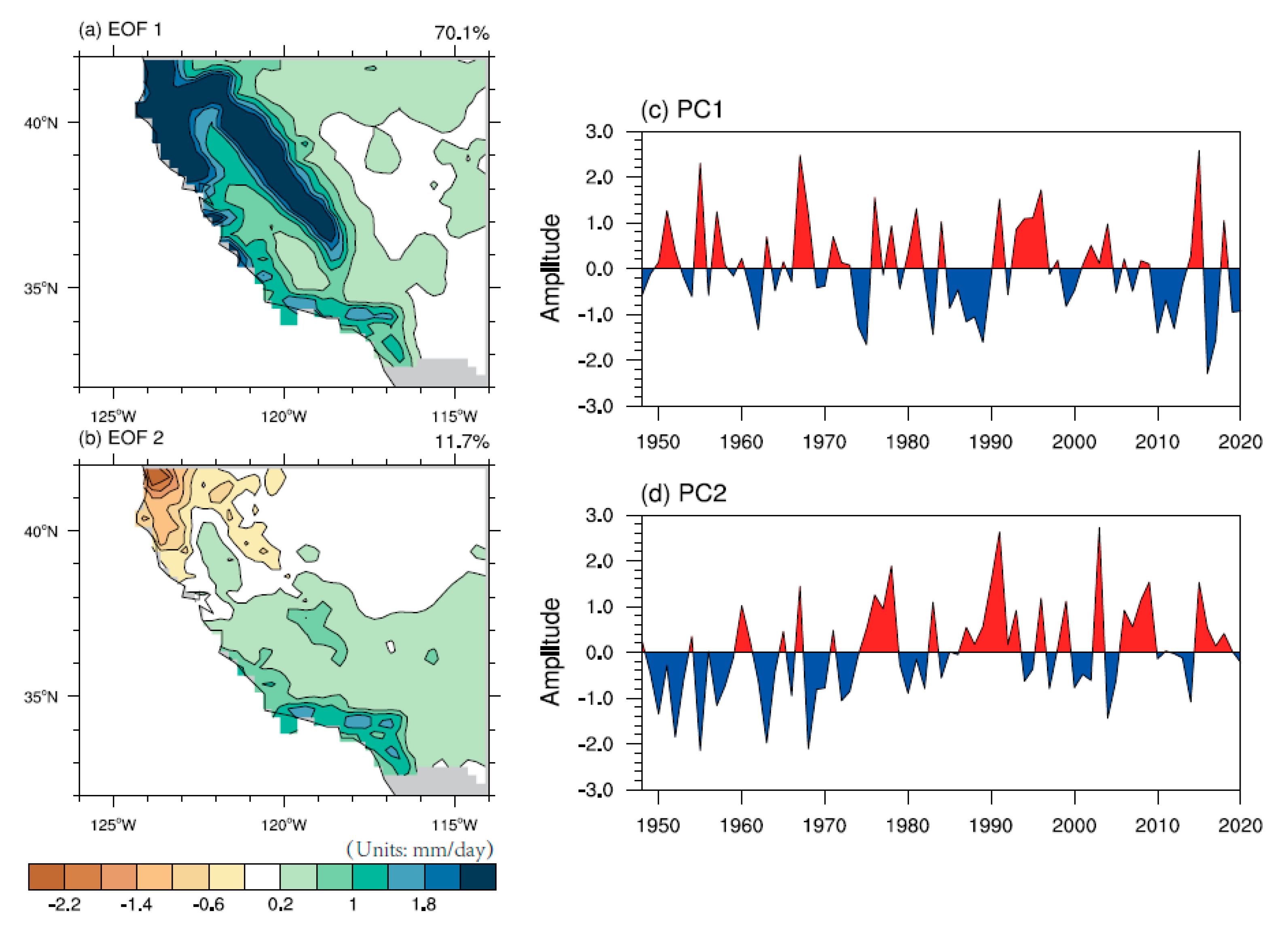
To identify the basic mode of precipitation evolution, empirical orthogonal function (EOF) analysis was applied. Figure 2 shows the leading two patterns and corresponding principal components (PCs). The first EOF pattern (EOF1) denoted a consistent evolution across the whole region. The variance contribution was 70.1%, indicating that the changes in California precipitation were mainly described by consistent changes. It is worth noting that there was seemingly a negative trend in the first principal component (PC1), indicating a general drying of California. In recent years, PC1has become more negative, representing the drought of California, which is consistent with observation. From the second EOF pattern (EOF2), a north–south dipole change in precipitation was shown, with opposite evolution between the north and south. The variance contribution was 11.7%. It is worth mentioning that there was an increasing trend in PC2, which may indicate that the south of California is becoming wetter, while the north is getting drier. The first two leading EOF modes were well separated from each other and the remaining modes, according to the criteria of North et al. (1982) [53]. Results reveal that these two patterns described two different processes and could be analyzed independently (figure not shown). The combination of EOF1 and EOF2 could explain over 80% of the precipitation change. Therefore, we only discuss the first two leading modes in this study.
4. Environmental Factors Affecting PC1 Changes
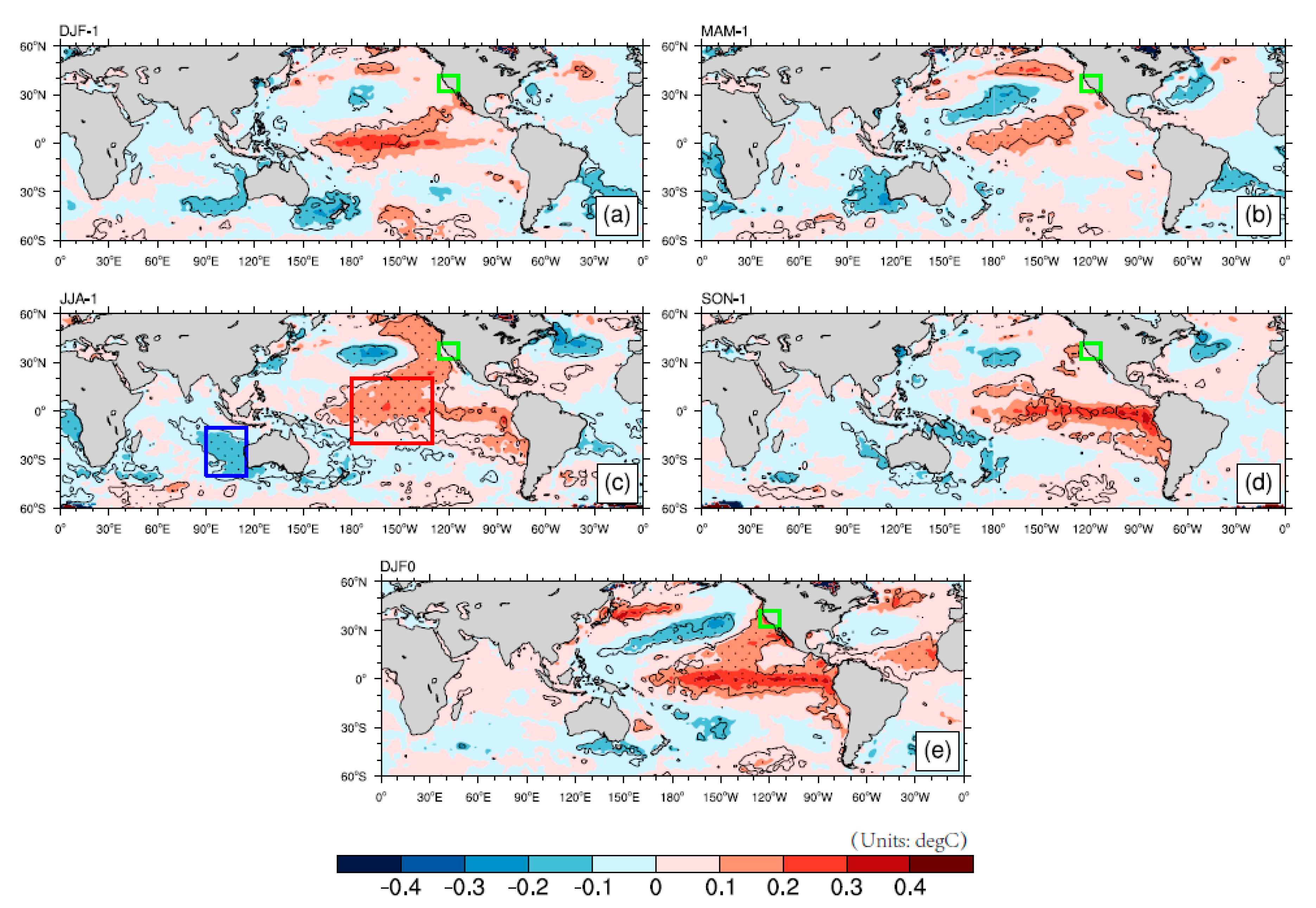
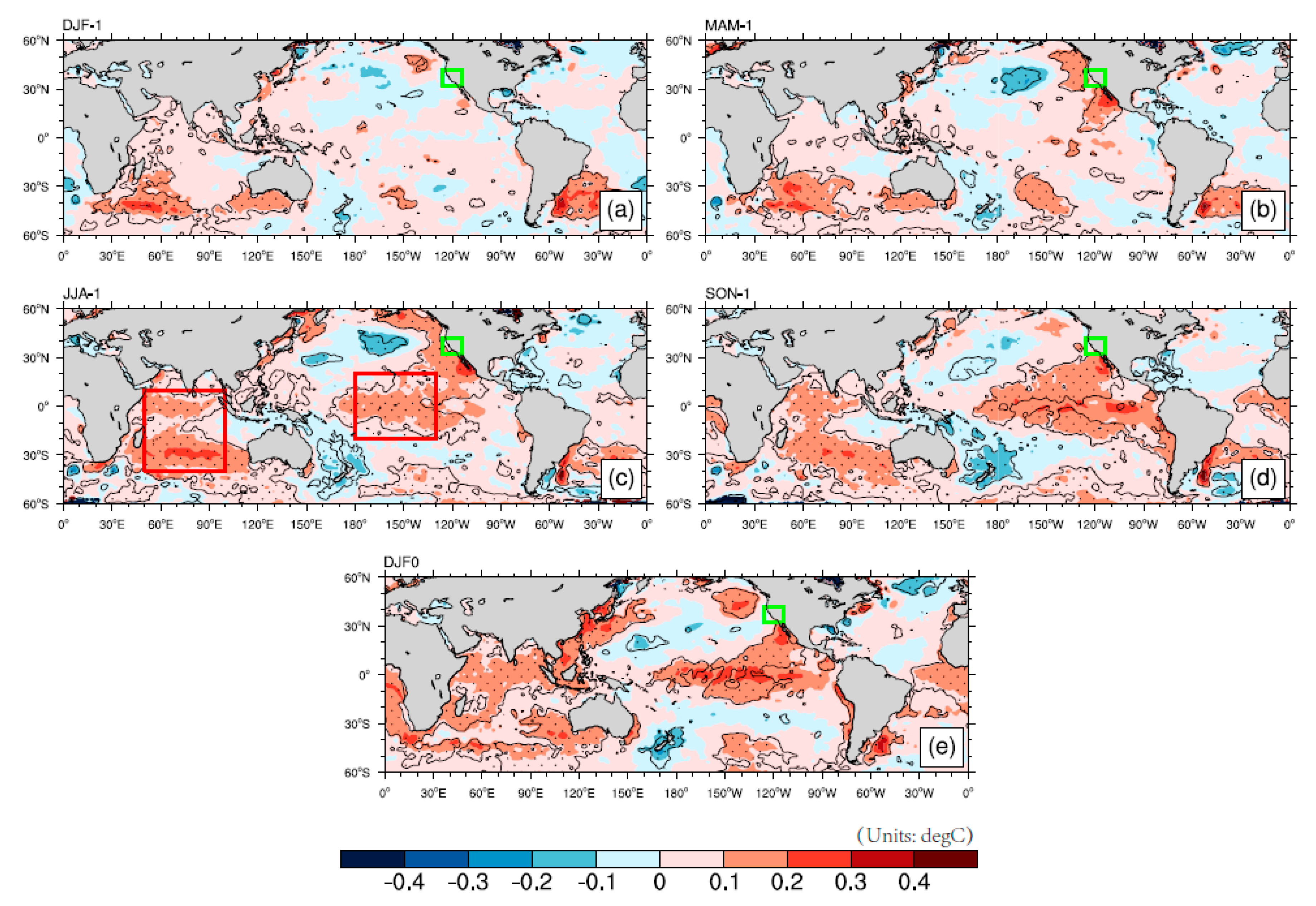
Since EOF1 and EOF2 described two different processes, the changes in PC1 and PC2 were analyzed separately. Figure 3 shows the evolution of SST patterns regressed to PC1 from the preceding winter to the subsequent winter. In both winters, we can see an El Niño-like pattern, which indicates that warm SST in the eastern Pacific Ocean corresponded to positive precipitation in California, consistent with previous studies [54]. It is worth noting that the positive relationship was continuous from the preceding winter to autumn. As the predictions of drought and flood are often needed one season in advance, and the signal in the preceding summer was most significant, the environmental factors were chosen in the preceding summer, as shown in Figure 3c. There was a positive relationship between SST in the central Pacific Ocean (red box; 20° S–20° N; 180–130° W) and California precipitation, as well as a negative relationship between SST in the southeast Indian Ocean (blue box; 40–10° S; 90–115° E) and California precipitation.
4.1. Central Pacific Ocean
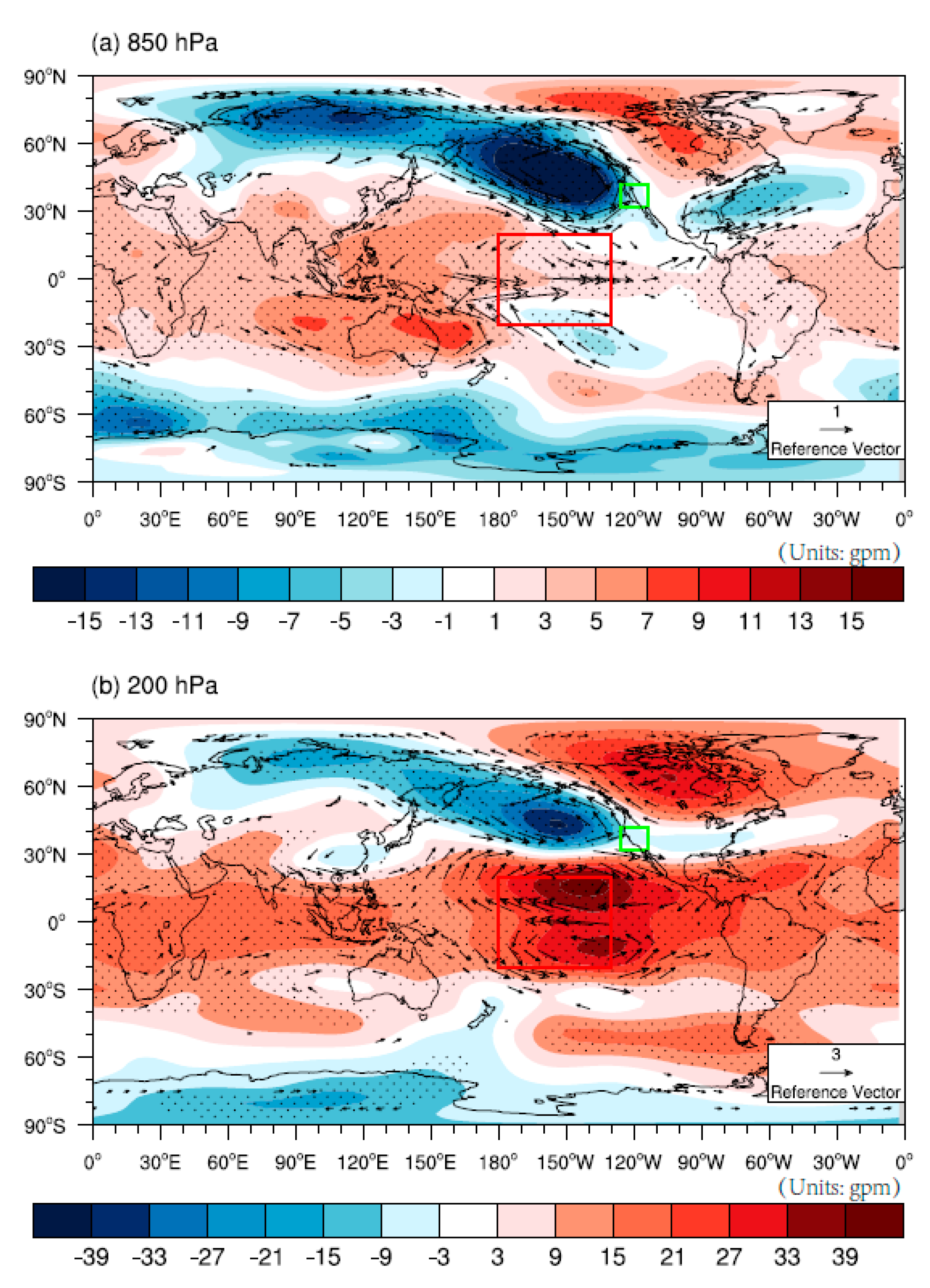
In order to investigate how the SST in the central Pacific Ocean influences California precipitation, index 1 was defined as the average SST over the significantly positive related region (red box in Figure 3c) in the preceding summer. Figure 4 shows the geopotential height and horizontal velocity at 850 hPa and 200 hPa in the subsequent winter regressed to index 1. From the figure, we can see that there was a Pacific Ocean–North America (PNA)-type response, induced by the positive SST in the central Pacific Ocean [39,40] at the lower level. There are four circulation centers from the north Pacific Ocean to the Atlantic Ocean. The key region (California) is located at the southeast of the cyclone and low-pressure anomaly centers. Accordingly, the region is occupied by southwesterly wind, which would transport warm and humid air from the Pacific Ocean. These characteristics could also be found at the upper level. In the mid-latitude region, the atmospheric systems are almost quasi-barotropic. Therefore, this region is also located at the southeast of the cyclone center and is occupied by southwesterly wind. The combination of the upper and lower levels induces favorable conditions for precipitation.
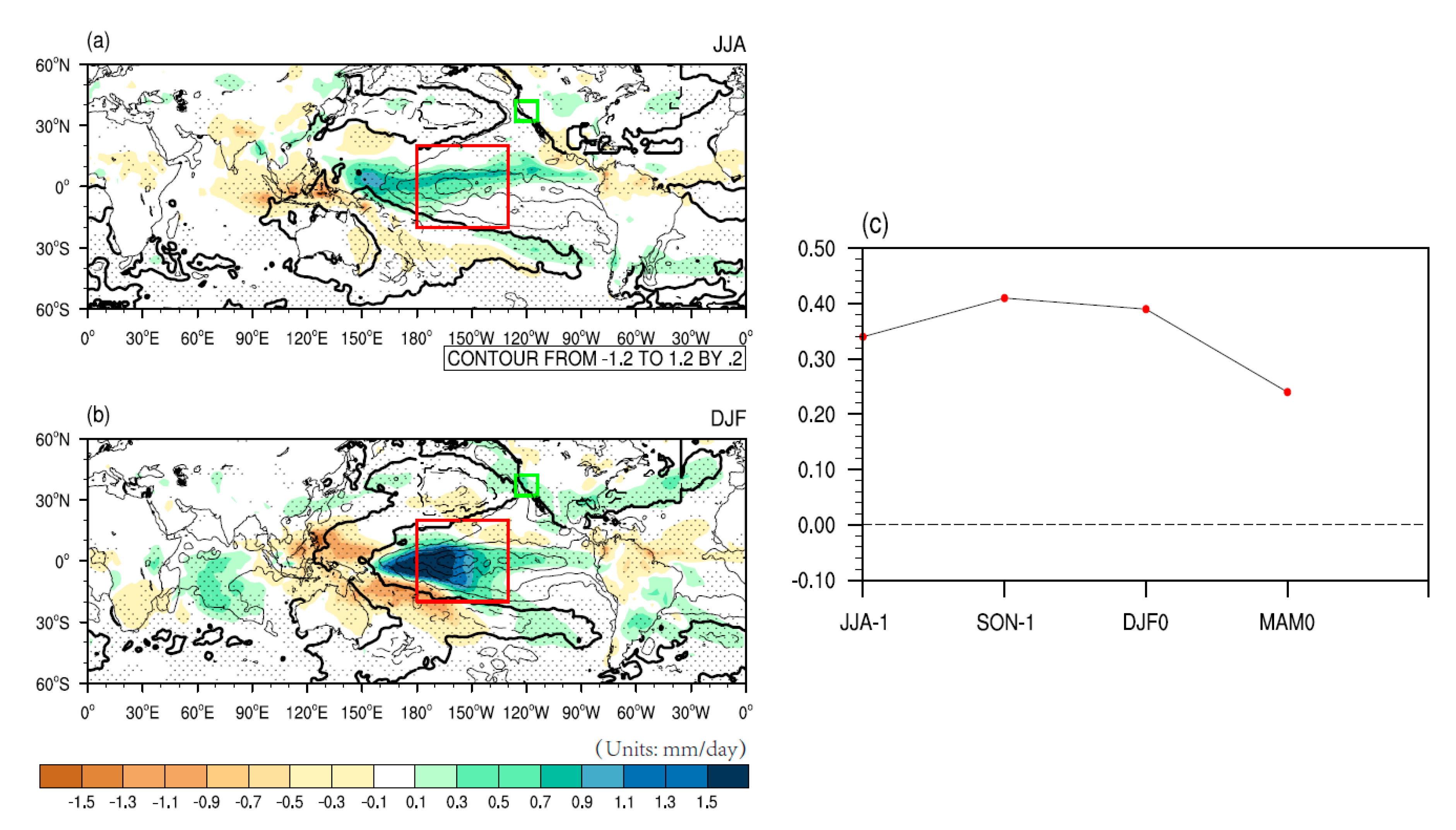
From the above analysis, we can infer that the positive SST in the central Pacific Ocean would cause positive precipitation in California. Next, we address how the signal in the preceding summer affects precipitation in the subsequent winter. We hypothesize that it is attributed to the slow change and persistence of SST. Figure 5 shows the precipitation and SST in the preceding summer and the subsequent winter regressed to index 1. The SST is positive in summer and changes slowly. According to air–sea interaction [55], induced by positive SST, the precipitation in the central Pacific is positive, leading to the PNA-like pattern response. Since the change in SST is slow, the SST is also positive in the subsequent winter, which would also cause PNA pattern and positive precipitation in the California region in the subsequent winter.
4.2. Southeast Indian Ocean
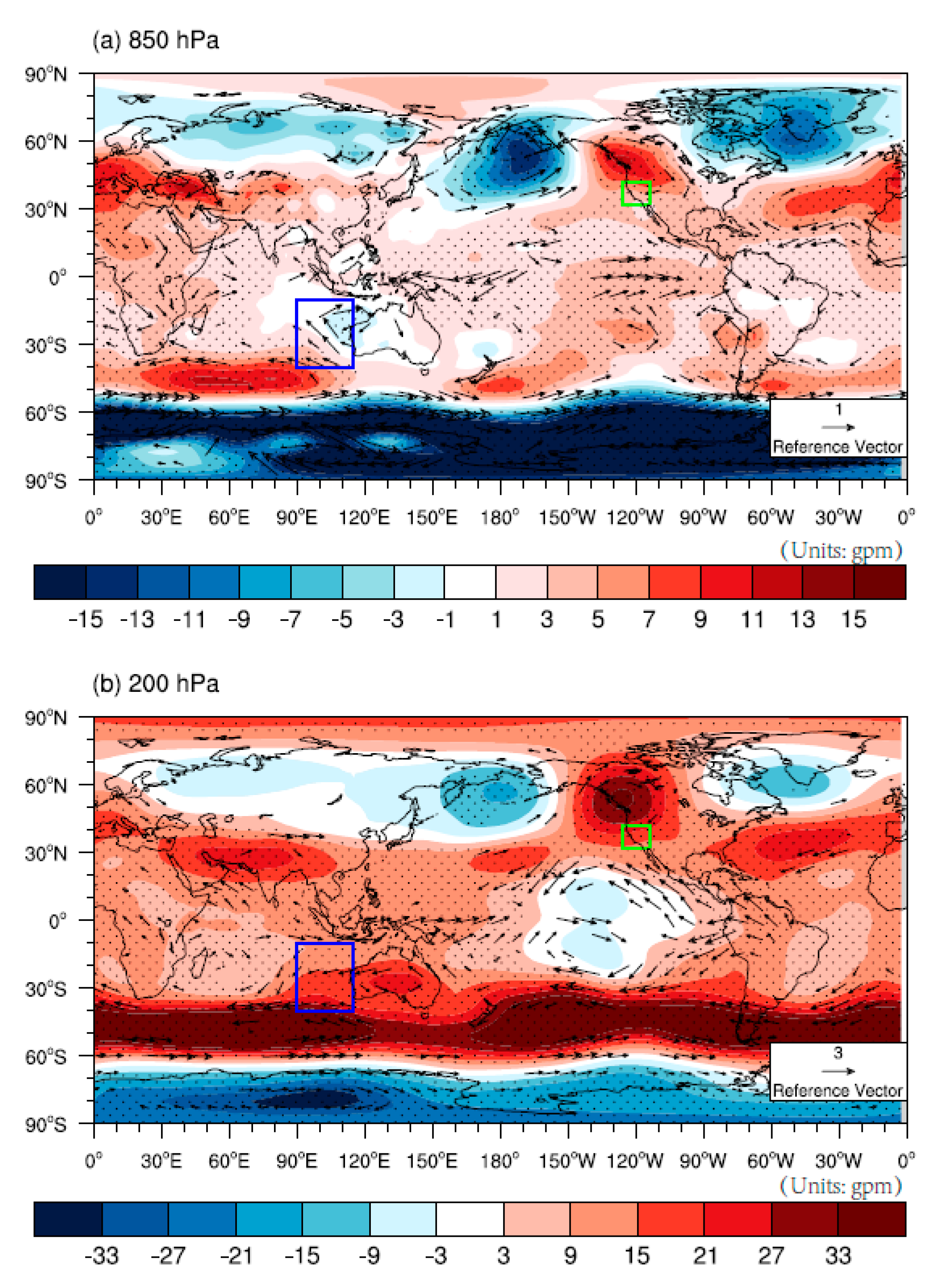
The relationship between SST in the southeast Indian Ocean and precipitation in California was negative. Using a similar method, index 2 was defined as the average SST in the blue box in Figure 3c in the preceding summer. Figure 6 shows the geopotential height and horizontal velocity at 850 hPa and 200 hPa in the concurrent winter regressed to index 2. Regardless of whether the lower level or upper level was considered, the key region was occupied by the significantly high pressure, leading to unfavorable conditions for precipitation and a negative relationship between SST in the Indian Ocean and precipitation in California, consistent with the above analysis. It is worth mentioning that the correlation coefficient between index 1 and index 2 was not significant (0.16), indicating that the Indian Ocean SST is an independent factor and has a negative contribution to California precipitation. Where is the source of the anticyclone? Here, we use wave activity and wave activity flux to describe this [56]. The definition of wave activity (W) is as follows:
where is horizontal wind, and are zonal and meridional velocity, denotes the stream function, , , and represent the climatology horizonal, zonal, and meridional velocity, and represents the anomalous stream function.
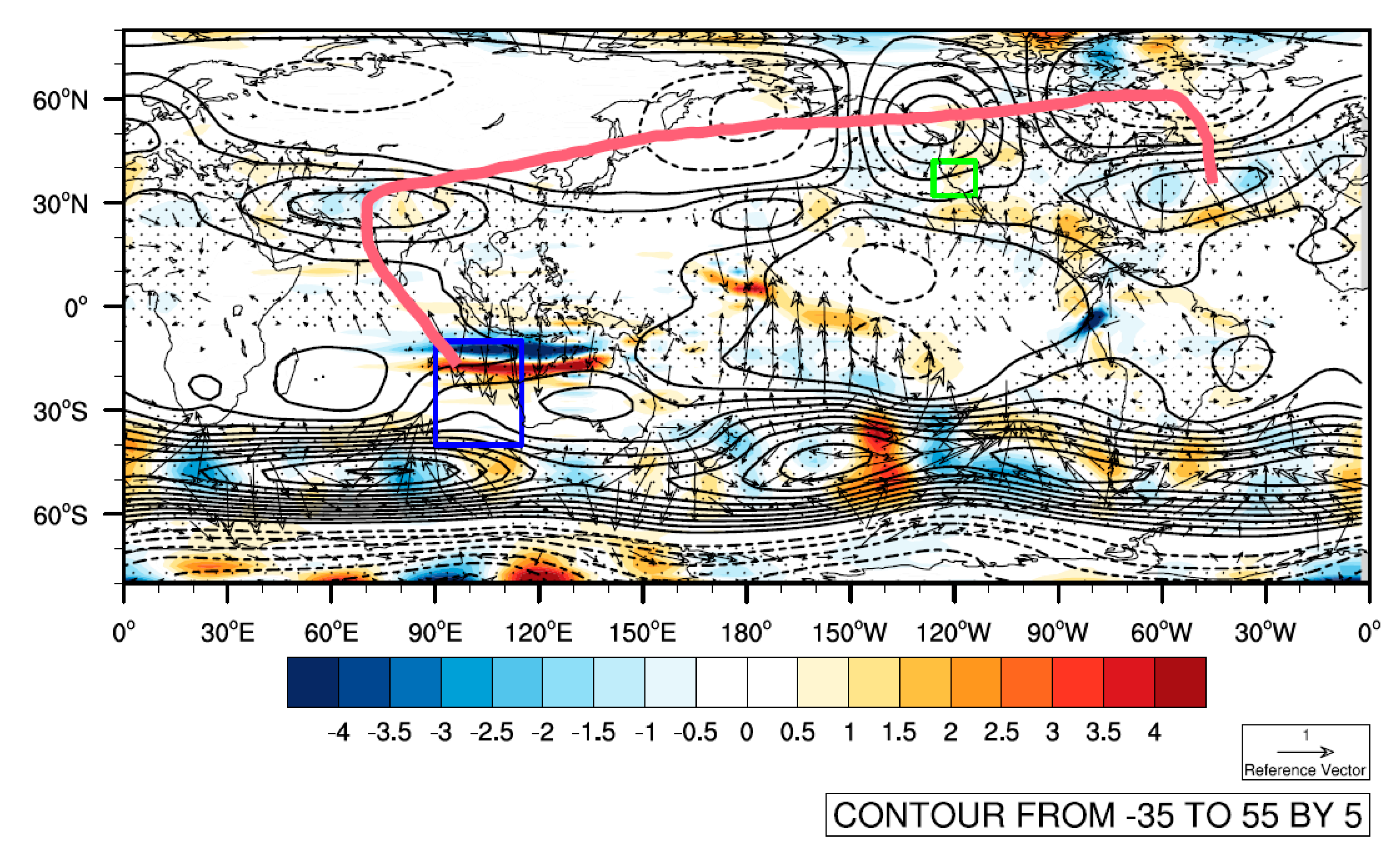
Figure 7 shows the wave activity flux. We can see that there is a Rossby wave source in the southeast Indian Ocean. The Rossby wave train extends from the northern Indian Ocean to the Atlantic Ocean. We can find an anticyclone and high-pressure anomaly in the northern Indian Ocean. California is controlled by the high-pressure anomaly, leading to a negative precipitation anomaly. In our opinion, the high-pressure anomaly and anticyclone in the northern Indian Ocean represent key systems and the Rossby wave source; hence, a positive SST in the southeast Indian Ocean could potentially lead to a cyclone at the lower level and an anticyclone at the upper level in the northern Indian Ocean. An anomaly GCM experiment was designed to address this possibility.
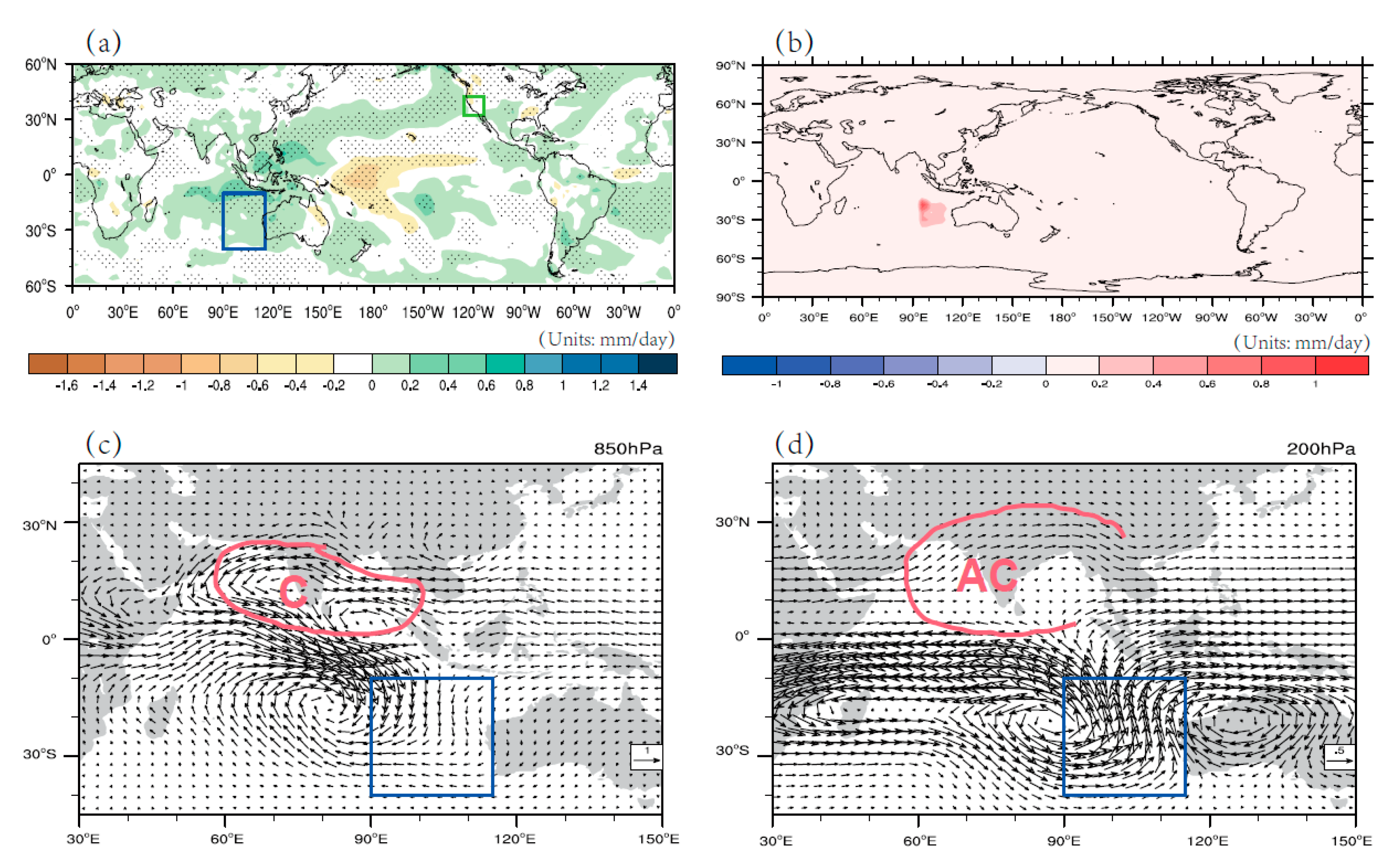
Figure 8a shows the regressed precipitation pattern. We can see that there was a positive precipitation anomaly in the east Indian Ocean. In order to determine the atmospheric response to this heating, only the precipitation anomaly in the key region was normalized and introduced into the AGCM, as shown in Figure 8b. From the model results (Figure 8c,d), we can see that there was cyclone at the lower level and an anticyclone at the upper level in the northern Indian ocean, consistent with the previous observation (Figure 6), induced by positive heating in the southeast Indian Ocean. According to the Gill response [57], even when the heating is asymmetric (such as a positive SST in the southeast Indian Ocean), there is also a cyclonic Rossby wave gyre response in the west at the lower level. In the tropics, the atmospheric system is baroclinic; thus, at the upper level, there would be an anticyclone in the northern Indian ocean. This, then, induces the Rossby wave train, resulting in an anticyclone and a high-pressure anomaly in California, which would cause negative precipitation.
5. Environmental Factors Affecting PC2 Changes
Figure 9 shows the evolution of SST patterns regressed to PC2 from the preceding winter to the subsequent winter. In both winters, we can see an El Niño-like pattern, which indicates that warm SST in the eastern Pacific Ocean corresponded to positive precipitation in California. Other than the decreased level of relevance, this characteristic was similar to PC1; thus, the environmental factors in the Pacific Ocean are not discussed here.
The situation was different in the Indian ocean. The relationship between PC2 and SST in the Indian Ocean in the preceding summer was significantly positive. In order to determine how the SST in the Indian Ocean influences California precipitation, index 3 was defined as the average SST in the mostly positive related region (40° S–10° N; 50–100° E; left red box in Figure 9c) in the preceding summer. Figure 10 shows the relative vorticity and horizontal velocity at 850 hPa and 200 hPa in winter regressed to index 3. From the figure, we can see that, at the upper level, the key region is controlled by positive vorticity and a cyclone, whereas at the lower level, the situation is complex. In the south of California, there is positive vorticity. Combined with circulation at the lower level, such positive vorticity is beneficial for positive precipitation. On the other hand, in the north of California, there is negative vorticity, which is unfavorable for precipitation. As a result, the combination of upper and lower circulation is favorable for precipitation in the south but unfavorable in the north, leading to a dipole mode of precipitation, which is consistent with EOF2.
6. Summary and Discussion
In this study, the environmental factors affecting precipitation in California during 1948–2020 were investigated. Considering the seasonal mean and standard deviation of precipitation, this paper focused on winter as the main rainy season with the greatest variation. According to the EOF analysis of winter precipitation, the first EOF mode described a consistent change, with a variance contribution of 70.1%. The second EOF mode exhibited a south–east dipole change with an 11.7% variance contribution.
For EOF1, the relationship was positive between SST in the central Pacific in the preceding summer with PC1 in winter and negative between SST in the southeast Indian Ocean in the preceding summer with PC1 in winter. Due to the slow change and continuity of SST, the warm SST in the central Pacific Ocean would be maintained from summer to winter. Thus, the positive precipitation induced would exist in the subsequent winter in the central Pacific Ocean, thereby inducing a PNA-type wave train response to influence the California precipitation. Regardless of whether the lower level or the upper level was considered, the key region was located to the southeast of the anomalous cyclone induced. The southwesterly wind would transport warm and wet flow from the ocean, beneficial for precipitation. There is another possible process underlying how warm SST in the central Pacific Ocean would affect California precipitation. California is located around the boundary of the tropical belt, at the edge of the Hadley cell sinking phenomenon. The edge of Hadley cells features a hot and dry climate. Yang et al. (2020) [58] proposed that poleward shift of the meridional temperature gradients would cause expanding tropics. Therefore, the El Nino-like pattern in EOF1 favors an equator contraction of the meridional temperature gradient, contributing to a narrower Hadley cell, which is then favorable for California precipitation. For the Indian ocean, the positive SST would induce an anomalous cyclone at the lower level and an anticyclone at the upper level in the northern Indian Ocean according to the Gill response. This was confirmed by both the observation and the AGCM model experiments. Following an anomalous heating in the eastern Indian Ocean in the model, there was a cyclone anomaly response at the lower level and an anticyclone anomaly response at the upper level in the northwest. The induced Rossby wave train extends from the Indian Ocean to the Atlantic Ocean. The key region is controlled by the biotrophically high pressure, which is unfavorable for precipitation.
As for PC2, the situation in Pacific Ocean was similar to that for PC1. There was a positive relationship between SST in the central Pacific Ocean in the preceding summer and California precipitation in winter. However, the circumstances were different in the Indian Ocean, whereby the relationship between SST in the Indian Ocean in the preceding summer and California precipitation in winter was also positive. Due to the slow change and continuity of SST, the warm SST would be maintained from summer to winter, which would induce a Rossby wave train from the Indian Ocean to California. Since the key region of the Indian Ocean is shifted westward, the wave train is shifted correspondingly. As a result, at the upper level, California is controlled by positive vorticity, whereas at the lower level, there is positive vorticity in the south and negative vorticity in the north. This combination of circulation at the upper and lower levels would lead to a dipole mode of precipitation, positive in the south and negative in the north.
It is worth mentioning that, in this study, how the summer conditions affect winter precipitation was mainly attributed to the slow change and continuity of SST. However, other possibilities, such as human activities, should be considered. Furthermore, only the effect of SST in the preceding summer was analyzed. Other environmental factors, such as geopotential height, in other seasons, such as in the preceding autumn, should also be considered. In this study, we only used AGCM to confirm the physical processes. Other models, such as ECHAM, should be applied. Further studies are needed to solve these questions. Having now found the precursor signals, further studies are needed to determine whether they can be adopted in precipitation forecasts.
Author Contributions
Data curation, L.Z.; formal analysis, F.H.; funding acquisition, L.Z.; methodology, Q.L.; validation, D.C.; writing—original draft, F.H.; writing—review and editing, F.H. All authors have read and agreed to the published version of the manuscript.
Funding
This work was jointly supported by the NSFC (grants 42088101 and 41875069), the China Scholarship Council (CSC) (grant N201908320493), and the Postgraduate Research and Practice Innovation Program of Jiangsu Province (grant SJKY19_0923).
Institutional Review Board Statement
Not applicable.
Informed Consent Statement
Not applicable.
Data Availability Statement
Datasets are available in a public repository that assigns persistent identifiers to datasets. 1. precipitation data used in this study are openly available from the Climate Prediction Center (CPC) at http://www.psl.noaa.gov/data/gridded/data.unified.daily.conus.html (accessed on 1 August 2021) as cited in Xie et al. 2007, ref. [41]. 2. precipitation data are openly available from the NOAA’s Precipitation Reconstruction Dataset (PREC) at https://www.esrl.noaa.gov/psd/data/gridded/data.prec.html (accessed on 1 August 2021) as cited in Chen et al. 2002, ref. [42]. 3. sea sur-face temperature (SST) data are openly available from the Hadley Center Global Sea Ice and Sea Surface Temperature dataset (HadISST) at http://www.metoffice.gov.uk/hadobs/hadisst (accessed on 1 August 2021) as cited in Rayner 2003, ref. [43]. 4. horizontal wind and geopotential height data are openly available from the National Centers for Environmental Prediction (NECP)/National Center for Atmosphere Research (NCAR) reanalysis http://www.esrl.noaa.gov/psd/data/gridded/data.ncep.reanalysis.html (accessed on 1 August 2021) as cited in Kalnay et al. 1996, ref. [44].
Conflicts of Interest
The authors declare no conflict of interest.
References
- Seager, R.; Hoerling, M.P.; Schubert, S.; Wang, H.; Lyon, B.; Kumar, A.; Nakamura, J.; Henderson, N. Causes of the 2011–2014 California Drought. J. Clim. 2015, 28, 6997–7024. [Google Scholar] [CrossRef]
- Diffenbaugh, N.S.; Swain, D.L.; Touma, D. Anthropogenic warming has increased drought risk in California. Proc. Natl. Acad. Sci. USA 2015, 112, 3931–3936. [Google Scholar] [CrossRef] [Green Version]
- US Census Bureau. State and County QuickFacts. 2014. Available online: Quickfacts.census.gov/qfd/states/06000.html (accessed on 20 March 2021).
- US Bureau of Economic Analysis. Bureau of Economic Analysis Interactive Data. 2014. Available online: www.bea.gov/ (accessed on 20 March 2021).
- US Department of Agriculture. CALIFORNIA Agricultural Statistics 2012 Crop Year. 2013. Available online: www.nass.usda.gov/Statistics_by_State/California/Publications/California_Ag_Statistics/Reports/2012cas-all.pdf (accessed on 20 March 2021).
- Zhu, Z.; Li, T. Amplified contiguous United States summer rainfall variability induced by East Asian monsoon interdecadal change. Clim. Dyn. 2017, 50, 1–14. [Google Scholar] [CrossRef]
- Manuel, J. Drought in the Southeast: Lessons for Water Management. Environ. Health Perspect. 2008, 116, A168–A171. [Google Scholar] [CrossRef] [PubMed] [Green Version]
- Gotvald, A.J.; Mccallum, B.E. Epic Flooding in Georgia, 2009. In U.S. Geological Survey Fact Sheet 2010-3107; U.S. Geological Survey: Reston, VA, USA, 2012; 2p. [Google Scholar]
- Griffin, D.; Anchukaitis, K.J. How unusual is the 2012–2014 California drought? Geophys. Res. Lett. 2014, 41, 9017–9023. [Google Scholar] [CrossRef] [Green Version]
- Williams, A.P.; Seager, R.; Abatzoglou, J.T.; Cook, B.I.; Smerdon, J.E.; Cook, E.R. Contribution of anthropogenic warming to California drought during 2012–2014. Geophys. Res. Lett. 2015, 42, 6819–6828. [Google Scholar] [CrossRef] [Green Version]
- Mao, Y.; Nijssen, B.; Lettenmaier, D.P. Is climate change implicated in the 2013–2014 California drought? A hydrologic perspective. Geophys. Res. Lett. 2015, 42, 2805–2813. [Google Scholar] [CrossRef]
- Nitta, T. Convective activities in the tropical western Pacific and their impact on the northern hemisphere summer circulation. J. Meteorol. Soc. Jpn. 1987, 65, 373–390. [Google Scholar] [CrossRef] [Green Version]
- Huang, R. The numerical simulation of the three-dimensional teleconnections in the summer circulation over the Northern Hemisphere. Adv. Atmos. Sci. 1985, 2, 81–92. [Google Scholar]
- Lau, K.M.; Weng, H. Recurrent Teleconnection Patterns Linking Summertime Precipitation Variability over East Asia and North America. J. Meteorol. Soc. Jpn. 2002, 80, 1309–1324. [Google Scholar] [CrossRef] [Green Version]
- Lau, K.M. Dynamics of atmospheric teleconnections during the Northern Hemisphere summer. J. Clim. 1992, 5, 140–158. [Google Scholar] [CrossRef] [Green Version]
- Ting, M.; Wang, H. Summertime, U.S. Precipitation Variability and Its Relation toPacific Sea Surface Temperature. J. Clim. 2010, 10, 1853–1873. [Google Scholar] [CrossRef]
- Hui, W.; Ting, M.; Ming, J. Prediction of seasonal mean United States precipitation based on El Niño sea surface temperatures. Geophys. Res. Lett. 1999, 26, 1341–1344. [Google Scholar]
- Li, C.; Zhang, L. Summer monsoon activities in South China Sea and its impacts. Chinese. Sci. Atmos. Sin. 1999, 3, 23. [Google Scholar]
- Lau, K.M. Dynamical and Boundary Forcing Characteristics of Regional Components of the Asian Summer Monsoon. J. Clim. 2000, 13, 2461–2482. [Google Scholar] [CrossRef]
- Wang, B.; Wu, R.; Lau, K.M. Interannual Variability of the Asian Summer Monsoon: Contrasts between the Indian and the Western North Pacific–East Asian Monsoons*. J. Clim. 2001, 14, 4073–4090. [Google Scholar] [CrossRef]
- Trenberth, K.E.; Guillemot, C.J. Physical Processes Involved in the 1988 Drought and 1993 Floods in North America. J. Clim. 1996, 9, 1288–1298. [Google Scholar] [CrossRef] [Green Version]
- Mo, K.C.; Paegle, J.N.; Higgins, R.W. Atmospheric Processes Associated with Summer Floods and Droughts in the Central United States. J. Clim. 1997, 10, 3028–3046. [Google Scholar] [CrossRef]
- Livezey, R.E.; Smith, T.M. Covariability of Aspects of North American Climate with Global Sea Surface Temperatures on Interannual to Interdecadal Timescales. J. Clim. 1999, 12, 289–302. [Google Scholar] [CrossRef]
- Mo, K.C. Intraseasonal Modulation of Summer Precipitation over North America. Mon. Weather Rev. 2000, 128, 1490–1505. [Google Scholar] [CrossRef]
- Higgins, R.W.; Leetmaa, A.; Xue, Y.; Barnston, A. Dominant factors influencing the seasonal predictability of United States precipitation and surface air temperature. J. Clim. 2000, 13, 3994–4017. [Google Scholar] [CrossRef] [Green Version]
- Ropelewski, C.F.; Halpert, M.S. North American Precipitation and Temperature Patterns Associated with the El Nio/Southern Oscillation (ENSO). Mon. Weather Rev. 1985, 114, 12. [Google Scholar]
- Palmer, T.N.; Brankovi, C. The 1988 US drought linked to anomalous sea surface temperature. Nature 1989, 338, 54–57. [Google Scholar] [CrossRef]
- Mo, K.C.; Schemm, J.E. Relationships between ENSO and drought over the southeastern United States. Geophys. Res. Lett. 2008, 35, 212–222. [Google Scholar] [CrossRef]
- Li, L.; Li, W.; Kushnir, Y. Variation of the North Atlantic subtropical high western ridge and its implication to Southeastern US summer precipitation. Clim. Dyn. 2012, 39, 1401–1412. [Google Scholar] [CrossRef] [Green Version]
- Dai, A. The influence of the inter-decadal Pacific oscillation on US precipitation during 1923–2010. Clim. Dyn. 2013, 41, 633–646. [Google Scholar] [CrossRef] [Green Version]
- Enfield, D.B. Relationships of inter-american rainfall to tropical Atlantic and Pacific SST variability. Geophys. Res. Lett. 1996, 23, 3305–3308. [Google Scholar] [CrossRef]
- Wang, H.; Fu, R.; Kumar, A.; Li, W. Intensification of Summer Rainfall Variability in the Southeastern United States during Recent Decades. J. Hydrometeorol. 2010, 11, 1007–1018. [Google Scholar] [CrossRef]
- Hu, Q.; Feng, S.; Oglesby, R.J. Variations in North American Summer Precipitation Driven by the Atlantic Multidecadal Oscillation. J. Clim. 2010, 1, 8. [Google Scholar] [CrossRef] [Green Version]
- Curtis, S. The Atlantic multidecadal oscillation and extreme daily precipitation over the US and Mexico during the hurricane season. Clim. Dyn. 2008, 30, 343–351. [Google Scholar] [CrossRef]
- McCabe, G.J.; Palecki, M.A.; Betancourt, J.L. Pacific and Atlantic Ocean influences on multidecadal drought frequency in the United States. Proc. Natl. Acad. Sci. USA 2004, 101, 4136–4141. [Google Scholar] [CrossRef] [PubMed] [Green Version]
- Horel, J.D.; Wallace, J.M. Planetary-Scale Atmospheric Phenomena Associated with the Southern Oscillation. Mon. Weather Rev. 1981, 109, 813–829. [Google Scholar] [CrossRef]
- Leathers, D.J.; Yarnal, B.; Palecki, M.A. The Pacific/North American Teleconnection Pattern and United States Climate. Part I: Regional Temperature and Precipitation Associations. J. Clim. 1991, 4, 517–528. [Google Scholar] [CrossRef]
- Trenberth, K.E.; Branstator, G.W.; Karoly, D.; Kumar, A.; Lau, N.C.; Ropelewski, C. Progress during TOGA in understanding and modeling global teleconnections associated with tropical sea surface temperatures. J. Geophys. Res. Ocean. 1998, 103, 14291–14324. [Google Scholar] [CrossRef]
- Coleman, J.S.M.; Rogers, J.C. Ohio River Valley Winter Moisture Conditions Associated with the Pacific–North American Teleconnection Pattern. J. Clim. 2003, 16, 969–981. [Google Scholar] [CrossRef]
- Ge, Y.; Gong, G.; Frei, A. Physical Mechanisms Linking the Winter Pacific–North American Teleconnection Pattern to Spring North American Snow Depth. J. Clim. 2009, 22, 5135–5148. [Google Scholar] [CrossRef] [Green Version]
- Xie, P.; Chen, M.; Yang, S.; Yatagai, A.; Hayasaka, T.; Fukushima, Y.; Liu, C. A Gauge-Based Analysis of Daily Precipitation over East Asia. J. Hydrometeorol. 2007, 8, 607–626. [Google Scholar] [CrossRef]
- Chen, M.; Xie, P.; Janowiak, J.E.; Arkin, P. Global Land Precipitation: A 50-yr Monthly Analysis Based on Gauge Observations. J. Hydrometeorol. 2002, 3, 249–266. [Google Scholar] [CrossRef]
- Rayner, N.A. Global analyses of sea surface temperature, sea ice, and night marine air temperature since the late nineteenth century. J. Geophys. Res. Atmos. 2003, 108, D14. [Google Scholar] [CrossRef]
- Kalnay, E.; Kanamitsu, M.; Kistler, R.; Collins, W.; Deaven, D.; Gandin, L.; Iredell, M.; Saha, S.; Whie, G.; Woolled, J.; et al. The NCEP/NCAR 40-year reanalysis project. Bull. Am. Meteorol. Soc. 1996, 77, 437–472. [Google Scholar] [CrossRef] [Green Version]
- Wei, F.Y. Modern Climate Statistical Diagnosis and Prediction Technology; China Meteorological Press: Beijing, China, 1956. [Google Scholar]
- Venkateshan, S.P. Regression Analysis. Mechanical Measurements; Springer International Publishing: Cham, Switzerland, 2021; pp. 49–77. [Google Scholar]
- Fisher, R.A. Accuracy of observation, A mathematical examination of the methods of determining, by the mean error and by the mean square error. Mon. Not. R. Astron. Soc. 1920, 80, 443–450. [Google Scholar] [CrossRef] [Green Version]
- Held, I.M.; Suarez, M.J. A proposal for the intercomparison of the dynamical cores of atmospheric general circulation models. Bull. Am. Meteorol. Soc. 1994, 75, 1825–1830. [Google Scholar] [CrossRef] [Green Version]
- Jiang, X.A.; Li, T. Reinitiation of the boreal summer intraseasonal oscillation in the tropical Indian Ocean. J. Clim. 2005, 18, 3777–3795. [Google Scholar] [CrossRef] [Green Version]
- Li, T.; Liu, P.; Fu, X.; Wang, B.; Meehl, G.A. Spatiotemporal Structures and Mechanisms of the Tropospheric Biennial Oscillation in the Indo-Pacific Warm Ocean Regions*. J. Clim. 2006, 19, 3070–3087. [Google Scholar] [CrossRef]
- North, G.R.; Bell, T.L.; Cahalan, R.F.; Moeng, F.J. Sampling Errors in the Estimation of Empirical Orthogonal Functions. Mon. Weather. Rev. 1982, 110, 699. [Google Scholar] [CrossRef]
- Bridge, N. The Climate of Southern California; University of California Press: Oakland, CA, USA, 1901. [Google Scholar]
- Wallace, J.M.; Gutzler, D.S. Teleconnections in the Geopotential Height Field during the Northern Hemisphere Winter. Mon. Weather Rev. 1981, 109, 784–812. [Google Scholar] [CrossRef]
- Barnston, A.G.; Livezey, R.E. Classification, Seasonality and Persistence of Low-Frequency Atmospheric Circulation Patterns. Mon. Weather Rev. 1987, 115, 1083–1126. [Google Scholar] [CrossRef]
- Lindzen, R.S.; Nigam, S. On the Role of Sea Surface Temperature Gradients in Forcing Low-Level Winds and Convergence in the Tropics. J. Atmos. Sci. 1987, 45, 2418–2436. [Google Scholar] [CrossRef] [Green Version]
- Nakamura, H.; Nakamura, M.; Anderson, J.L. The Role of High- and Low-Frequency Dynamics in Blocking Formation. Mon. Weather Rev. 1997, 125, 2074–2093. [Google Scholar] [CrossRef] [Green Version]
- Gill, A.E. Some simple solutions for heat-induced tropical circulation. Q. J. R. Meteorol. Soc. 2010, 106, 447–462. [Google Scholar] [CrossRef]
- Yang, H.; Lohmann, G.; Lu, J.; Gowan, E.J.; Shi, X.; Liu, J.; Wang, Q. Tropical Expansion Driven by Poleward Advancing Midlatitude Meridional Temperature Gradients. J. Geophys. Res. Atmos. 2020, 125, e2020JD033158. [Google Scholar] [CrossRef]
Figure 1.
Seasonal anomalies (a–d; mm/day) and standard deviation (e–h) of precipitation in winter (a,e), spring (b,f), summer (c,g), and autumn (d,h) during 1948–2020. The climatology is based on the time period of 1951–1990 over land and 1979–1998 over oceans. Shading denotes altitude (m). Box-averaged variables are shown above each panel.

Figure 2.
Patterns (a,b; mm/day) and principal components (c,d) of first (a,c) and second (b,d) EOF modes of winter precipitation anomalies.
Figure 2.
Patterns (a,b; mm/day) and principal components (c,d) of first (a,c) and second (b,d) EOF modes of winter precipitation anomalies.

Figure 3.
Evolution of SST patterns (°C) regressed to standardized PC1 from the preceding winter (a) to spring (b), summer (c), autumn (d) and the subsequent winter (e). Areas with dots exceed a 90% confidence level. The green box represents the selected California area. Red and blue boxes denote key regions analyzed.

Figure 4.
Geopotential height (shading; gpm) and horizontal velocity (vector; m/s) at 850 hPa (a) and 200 hPa (b) in winter regressed to the box-averaged SST (red box). The green box represents the selected California area. Only wind exceeding the 90% confidence level is shown. Areas with dots exceed the 90% confidence level.

Figure 5.
Precipitation (shading; mm/day) and SST (contour; °C) in the preceding summer (a) and subsequent winter (b) regressed to the box-averaged SST (red box). The green box represents the selected California area. (c) Time evolution of box-averaged SST (°C) from the preceding summer to subsequent spring. Areas with dots exceed the 90% confidence level.

Figure 6.
Same as in Figure 4, except that SST is averaged over the blue box.
Figure 6.
Same as in Figure 4, except that SST is averaged over the blue box.

Figure 7.
Geopotential height (contour; gpm), wave activity (vector; m/s), and wave activity flux (shading; s−1) at 200 hPa (bottom) in winter regressed to the box-averaged SST (blue box). The red line highlights the wave train. The green box represents the selected California area. Only the wave activity exceeding the 90% confidence level is shown. Areas with dots exceed the 90% confidence level.

Figure 8.
(a) Precipitation (mm/day) in winter regressed to the box-averaged SST (blue box). The green box represents the selected California area. Areas with dots exceed the 90% confidence level. (b) Diabatic heating anomaly pattern introduced into the AGCM experiment. Atmospheric response (m/s) at 850 hPa (c) and 200 hPa (d) in the model. “C” and “AC” represent the anomalous cyclone and anticyclone induced.

Figure 9.
Same as in Figure 3, except for PC2.
Figure 9.
Same as in Figure 3, except for PC2.

Figure 10.
Relative vorticity (shading; 10−7 s−1) and horizontal velocity (vector; m/s) at 850 hPa (a) and 200 hPa (b) in winter regressed to the box-averaged SST (the left red box in Figure 9c). The green box represents the selected California area. Areas with dots exceed the 90% confidence level.
Figure 10.
Relative vorticity (shading; 10−7 s−1) and horizontal velocity (vector; m/s) at 850 hPa (a) and 200 hPa (b) in winter regressed to the box-averaged SST (the left red box in Figure 9c). The green box represents the selected California area. Areas with dots exceed the 90% confidence level.

Publisher’s Note: MDPI stays neutral with regard to jurisdictional claims in published maps and institutional affiliations. |
© 2021 by the authors. Licensee MDPI, Basel, Switzerland. This article is an open access article distributed under the terms and conditions of the Creative Commons Attribution (CC BY) license (https://creativecommons.org/licenses/by/4.0/).
Share and Cite
MDPI and ACS Style
Hu, F.; Zhang, L.; Liu, Q.; Chyi, D. Environmental Factors Controlling the Precipitation in California. Atmosphere 2021, 12, 997. https://0-doi-org.brum.beds.ac.uk/10.3390/atmos12080997
AMA Style
Hu F, Zhang L, Liu Q, Chyi D. Environmental Factors Controlling the Precipitation in California. Atmosphere. 2021; 12(8):997. https://0-doi-org.brum.beds.ac.uk/10.3390/atmos12080997
Chicago/Turabian StyleHu, Feng, Leying Zhang, Qiao Liu, and Dorina Chyi. 2021. "Environmental Factors Controlling the Precipitation in California" Atmosphere 12, no. 8: 997. https://0-doi-org.brum.beds.ac.uk/10.3390/atmos12080997
Note that from the first issue of 2016, this journal uses article numbers instead of page numbers. See further details here.