1. Introduction
More than half of the world’s population lives in urban areas and the danger from an accidental or deliberate release of hazardous materials can be significant. The transport and dispersion of atmospheric contaminants in urban areas is strongly influenced by surrounding buildings, which significantly modify the winds, leading to areas of channeling along the streets, updrafts and downdrafts in the wake of the buildings, and recirculating flow in street canyons [
1,
2]. In addition, urban areas create highly heterogeneous regions of wind speed and turbulence intensity. Similarly in complex terrain, the local terrain impacts the flow field significantly, producing similar complex effects which can lead to non-intuitive dispersion patterns. There is a great need to have an accurate and efficient capability to predict dispersion and deposition patterns in these complex scenarios.
High-resolution computer models can predict how airborne materials spread around buildings in urban areas and land features in complex terrain. However, the modeling tool must be flexible enough to use for a variety of applications, and should be coupled to many relevant databases, such as terrain, building shapefiles, land-use characteristics, and population. Many fast-response urban dispersion models have been developed to predict transport for these scenarios. Gaussian plume models, which run in seconds on a laptop, have been modified to account for the plume centerline shift that may occur due to channeling in street canyons [
3]. Hall et al. (2000) developed a Gaussian puff model called the Urban Dispersion Model (UDM) for use from neighborhood to city scales [
4]. Röckle (1990) derived a diagnostic model that computes three-dimensional (3-D) flow around buildings using empirical equations and mass conservation [
5]. Most fast-response models rely on empirical algorithms based on idealized building configurations. This makes it difficult to generalize the accuracy of these models for flow fields in highly heterogeneous urban terrain without many validation exercises [
6].
Computational fluid dynamics (CFD) models have been used to compute the flow field in urban areas and complex topography. Comparison of these results with field measurements shows that these models work well in most regions [
7,
8,
9,
10,
11,
12,
13]. These CFD models, however, are computationally very expensive and prohibitive for applications related to toxic releases in cities or at industrial facilities where turnaround time is very important.
Further, before running CFD models, users need to generate detailed grids that account for the 3-D geometry of the surrounding city and terrain. This is usually a time-consuming process, which renders these models useless for an operational response where a quick answer is needed in a small amount of time.
Gowardhan et al. (2011) developed a fast-response CFD model which represents an intermediate model type that produces fast runtimes (in the order of minutes for a several-block problem) and a reasonably accurate solution [
9]. Neophytou et al. (2011) also evaluated this model and showed these fast-response CFD models can accurately predict the flow features in complex urban configurations [
10].
Based on work carried out by Gowardhan (2008) and Gowardhan et al. (2011), we have developed a new fast-response operational dispersion modeling system called Aeolus, which can predict the flow and transport of airborne contaminants in urban areas and complex terrain [
9,
11]. The model can be run in a very efficient (~minutes) RANS (Reynolds average Navier–Stokes) mode or a detailed (~hours) LES (large eddy simulation) mode.
In this paper, we describe the Aeolus model and evaluate its performance in large eddy simulation mode. The LES version is validated for two different cases and applied to a third case to showcase the model capabilities over a wide range of applications. We first present validation results for turbulence generated in neutrally stratified flow over complex terrain case using data from Askervien hill campaign [
14]. Next, flow and dispersion in an urban area is validated using wind and tracer data from the Joint Urban 2003 Oklahoma City field experiment [
15]. Last, we apply the model’s capability to simulate the cloud rise dynamics of a high-temperature bubble from a nuclear explosion in the troposphere using data from the Upshot-Knothole Dixie test. This test was a high-altitude air burst with an explosive yield of 11 kilotons and a height of burst (HOB) of 1836 m above ground level (AGL).
2. Introduction to Aeolus Modeling System
Aeolus is an efficient 3-D CFD code based on a finite volume method. It solves the time-dependent incompressible Navier–Stokes equations on a regular cartesian staggered grid using a fractional step method algorithm. It also solves a scalar transport equation for potential temperature, which is coupled to the flow using an anelastic approximation. The model includes a Lagrangian dispersion model for predicting the atmospheric transport and dispersion of tracers and other materials. The RANS version of Aeolus is used as an operational model in the National Atmospheric Release Advisory Center (NARAC) at Lawrence Livermore National Laboratory (LLNL) for quickly simulating the impacts of airborne hazardous materials in urban areas. NARAC uses Aeolus and other operational atmospheric models to provide the United States Department of Energy information and services pertaining to chemical, biological, radiological, and nuclear airborne hazards [
16,
17]. NARAC can simulate downwind effects from a variety of scenarios, including fires, industrial and transportation accidents, radiation dispersal device explosions, hazardous material spills, sprayers, nuclear power plant accidents, and nuclear detonations.
2.1. Large Eddy Simulation Model
Aeolus can be run in a high-fidelity mode using an LES model. LES resolves the time-dependent turbulent flow field at both small and large scales, allowing better fidelity than alternative approaches such as RANS. The smallest scales of the solution rely on a Smagorinsky model with a constant of Cs = 0.12 to account for unresolved scales in the flow, rather than resolving them directly as in expensive direct numerical simulation (DNS) methods. This makes the computational cost for applying LES to realistic engineering systems with complex geometry or flow configurations practical and attainable using supercomputers. In contrast, direct numerical simulation, which resolves every scale of the solution, is prohibitively expensive for nearly all atmospheric dispersion problems with complex geometry.
2.2. Numerics
The model uses the 3rd order accurate Quadratic Upstream Interpolation for Convective Kinematics (QUICK) scheme [
18] for the advective terms and 2nd order central difference for the diffusive terms. The scalar transport equation uses a Bounded QUICK (BQUICK) scheme to obtain a bounded solution while maintaining spatial accuracy and reducing dispersion errors. The law of the wall boundary condition is imposed at the rigid surface by applying a free slip boundary condition at the surface. The tangential shear stress is set equal to
u∗2. The value of friction velocity
u∗ is evaluated using a log-law (
u∗ =
uk/ln(0.5 × Δ
z/
z0)), where
u is the magnitude of the tangential velocity and
z0 is the surface roughness, k is the von Karman constant with a value of 0.4, and Δ
z is the vertical grid resolution.
The pressure Poisson equation is solved using the successive over-relaxation method (SOR via the methodology described above). A free slip condition is used at the top and side boundaries. The following outflow boundary condition is prescribed at the outlet:
where
denotes the direction normal to the boundary face, φ is the advected variable, and
Ub is a velocity that is independent of the location of the outflow surface and is selected so that an overall mass balance is maintained. This boundary condition allows the convection of turbulent structures out of the domain and avoids problems with reflection of pressure waves back to the interior of the domain.
2.3. Dispersion Model
To model dispersion within the atmosphere, Aeolus models the 3-D, incompressible, advection–diffusion equation with sources and sinks using a Lagrangian framework [
19]:
where the total derivative represents the advection and diffusion that occurs to species in a Lagrangian reference frame,
is the air concentration of the species,
Q is the source term, and
S is the sink term, which accounts for removal processes such as deposition.
The equations for the Lagrangian particle displacement due to advection, diffusion, and settling in the three coordinate directions are:
where
is the wind components in the
x,
y, and
z projection directions, respectively,
is the eddy diffusivity,
is the Schmidt number,
dWx,y,z are three independent normal random variates with zero mean and variance
dt, which is the timestep of advection of the Lagrangian particle. The stochastic differential equations above are then integrated in time to calculate an independent trajectory for each Lagrangian particle. The concentration
, at any time
t, can then be calculated from the Lagrangian particle locations at time
t and the contaminant mass associated with each particle. The model does not apply kernel smoothing and the grid cell concentration depends on the number of particles in the respective grid cell.
2.4. Grid Generation
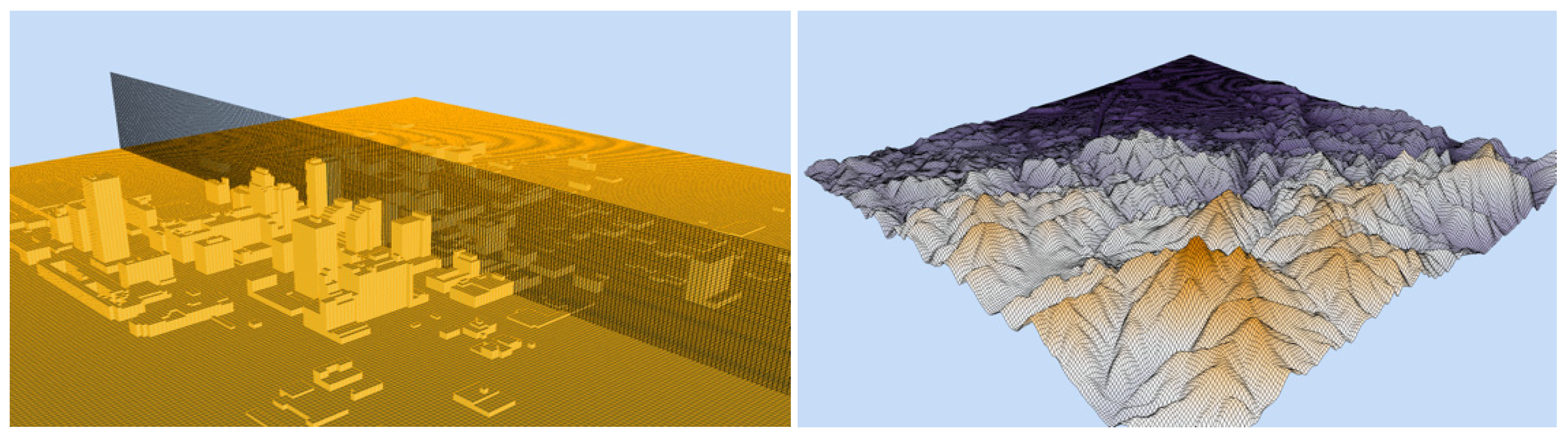
The model uses a cartesian grid and straightforward masking approach for generating a computational grid. New model grids can be generated in seconds from geographic information system shapefiles (for a few kilometers) and/or building data available from the National Geospatial Intelligence Agency and United States Geological Service (USGS) dataset containing building data for over 100 U.S. cities. Apart from the building dataset, the model also uses the USGS national elevation data at 10 m resolution (NED10) for terrain information which covers the 48 contiguous U.S. states, Hawaii, and portions of Alaska. The built-in datasets and fast grid generation tools are useful for operational applications. Examples of the grids produced for urban areas and complex terrain areas are shown in
Figure 1.
Apart from the elevation and building databases, the modeling system also integrates data about land-use characteristics, daytime and nighttime population, as well as meteorological fields from operational weather forecast centers and other sources. All the above information provides the model with the required initial and boundary conditions and subsequently helps to reduce the model setup time to minutes. The integrated databases also ensure that relevant products can be produced quickly and be distributed to relevant authorities.
2.5. Inflow Turbulence
Large eddy simulation models often need a precursor simulation to build a turbulent inflow profile. However, this process can be time consuming and difficult to achieve in an operational setup. Following DeLeon and Senocak (2017), we have developed a robust inflow turbulence generator which uses temperature perturbations in cells near the inflow boundary to produce a turbulent profile [
20]. The inflow turbulence zone is contained within the five grid cells nearest to the inlet where a mean velocity is prescribed. The buoyancy effect due to the perturbation in the temperature field propagates to the velocity field and produces the requisite turbulent structures.
3. Complex Terrain Validation
The Aeolus model using the large eddy simulation methodology was validated against experimental data for three different applications: flow over complex terrain, flow and dispersion of tracers in urban areas, and cloud rise dynamics for buoyant plumes from high-temperature explosions. This section covers the complex terrain validation, while the following two sections cover the urban area and cloud rise validations.
The Askervein Hill project [
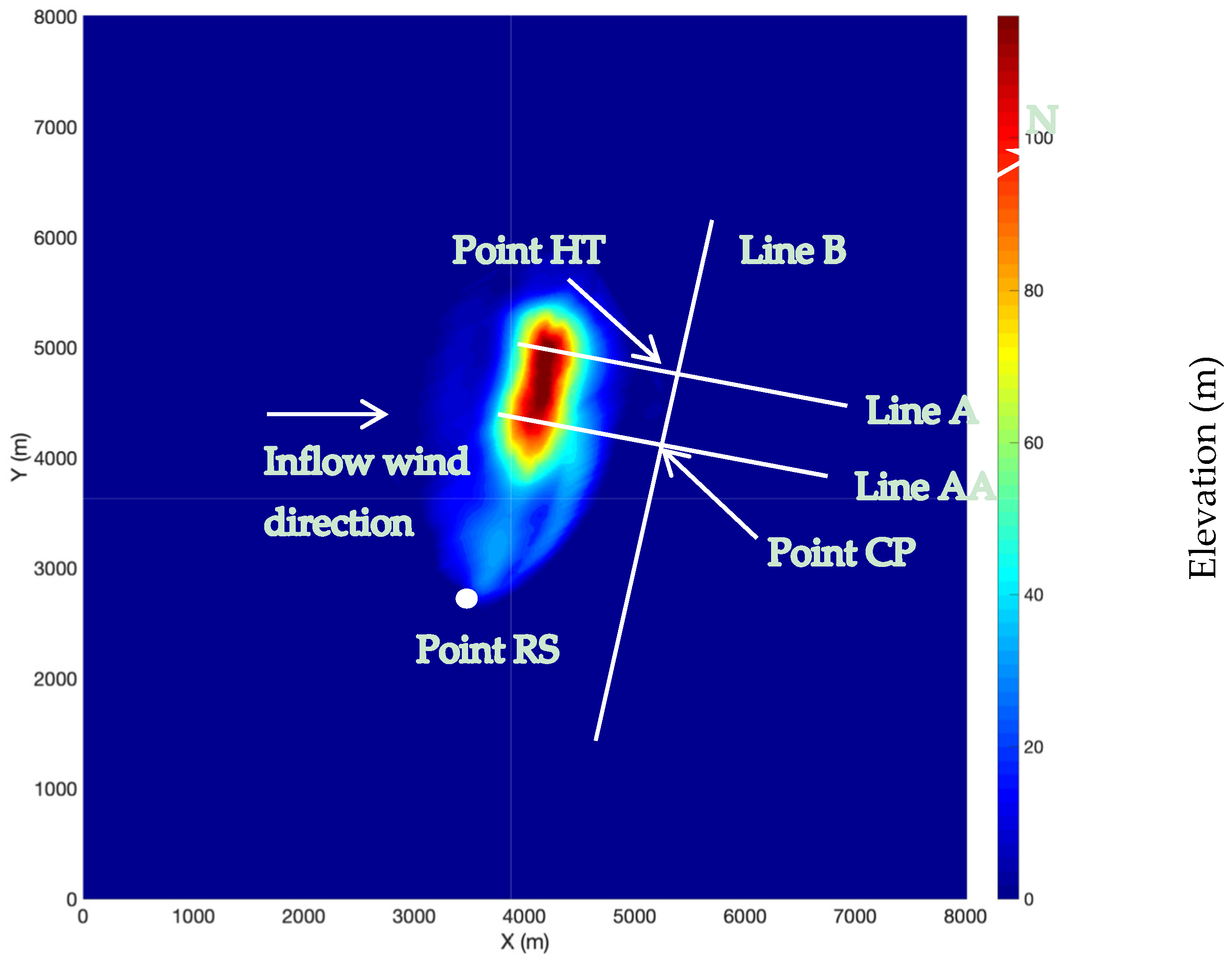
14] was a field study conducted in 1982 and 1983 to study the boundary-layer flow over low-profile hills. It was performed under a collaborative effort under the auspices of the International Energy Agency Programme for Research and Development on Wind Energy Conversion Systems. Askervein Hill is a low, isolated elliptic hill on the west coast of the island of South Uist in the Outer Hebrides of Scotland, which peaks at about 116 m above the ground. During these field campaigns, more than 50 towers were deployed and instrumented for wind measurements on and around this low-profile hill, as shown in
Figure 2. Towers were placed in two arrays along the major axis of the hill (lines A and AA), in the prevailing wind direction, and one array along the minor axis of the hill (line B). Lines A and AA pass through points hilltop (HT) and center point (CP), respectively, and along an orthogonal line B. A measurement site called reference site (RS) was also placed upstream of the hill to characterize the inflow conditions.
The Aeolus grid was generated by rotating the elevation dataset clockwise by 60 degrees so that the inflow wind direction is orthogonal to the grid as shown in
Figure 2, with the vertical extent of 1 km. A uniform Cartesian mesh was created using a grid resolution of Δ
x, Δ
y = 20 m, and Δ
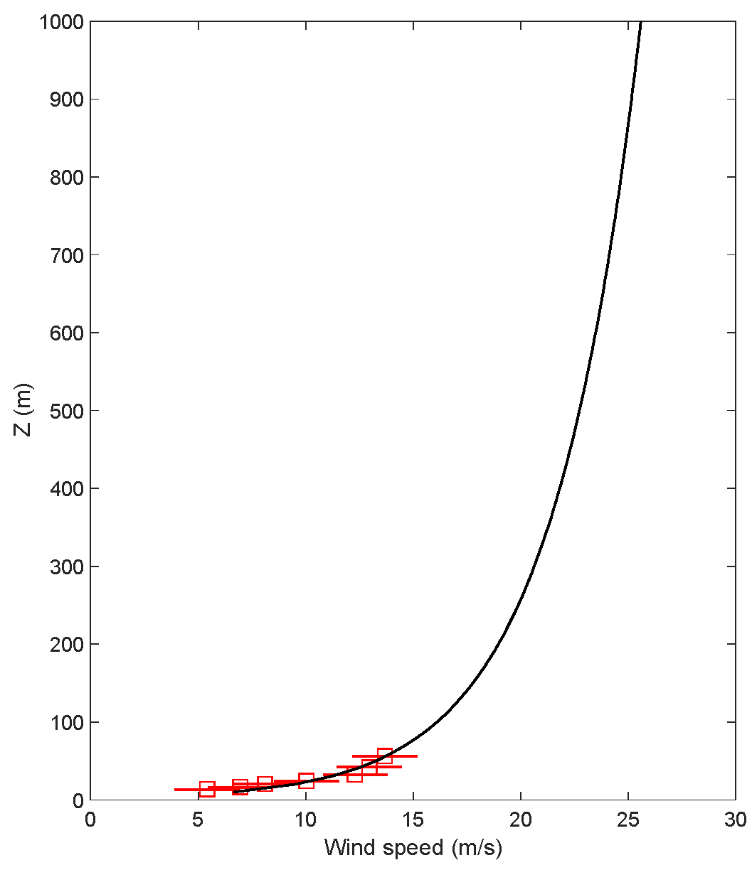
z = 10 m resulting in~16 million grid cells. The inflow velocity profile was created using a log-law profile (
u = (
u∗/
k) ln(
z/
z0)), to fit the observed data from the upstream site RS as shown in
Figure 3. The value of surface roughness,
z0, was 0.03 m [
14] and the friction velocity
u∗ was derived using the velocity reading (
ur = 14 m/s at
zr = 60 m) at the reference site RS.
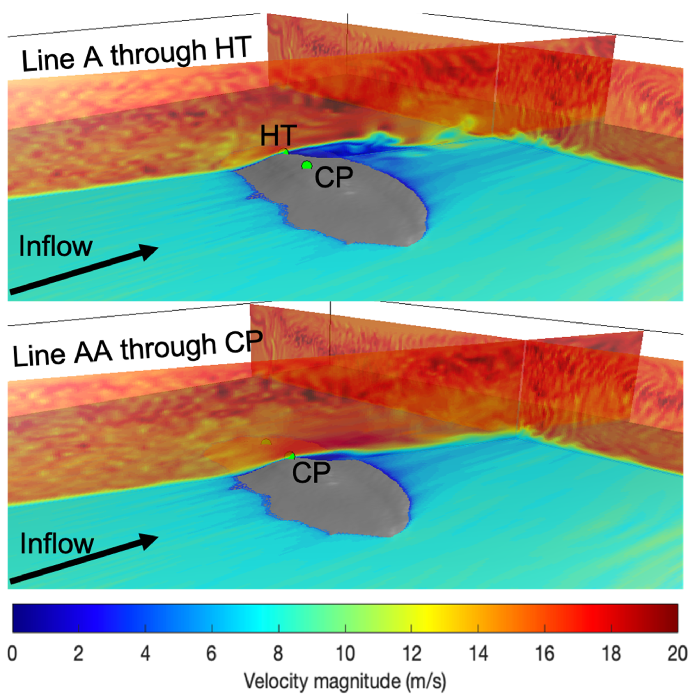
Figure 4 shows the turbulent structures in the velocity magnitude in a vertical slice along lines A and AA. The velocity magnitude increases as it passes over the Askervein Hill top and the flow separates in the lee side of the hill. It can be observed that a larger wake is created behind the plane passing along line A. This larger region of separation occurs due to a steeper drop in elevation along line A and has been observed in other model results, as well as observed data.
Winds were simulated for 2 h, which took about 6 h of computer time on a quad-core machine. After a 1.5 h spinup period, Aeolus data from the last 30 min of the simulation was time averaged for comparision with the observed data.
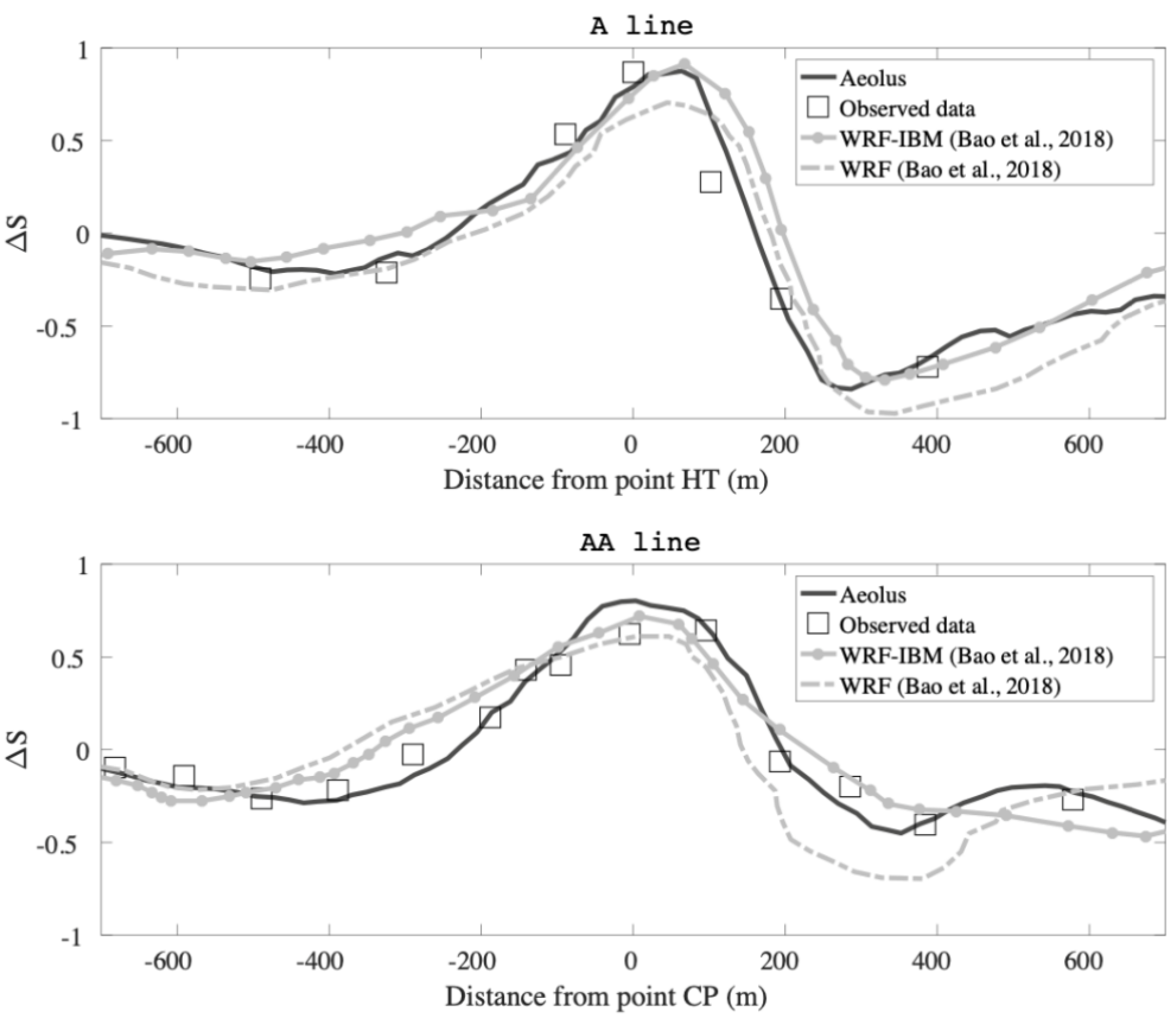
Observations along lines A and AA are compared with averaged velocities from the Aeolus simulation. Historically, other model simulations have been compared to the Askervein Hill dataset in terms of fractional speedup
, which is defined as
where
S is the horizontal wind speed at a specified height above the surface
z = 10 m, and
SRS is the wind speed at the reference site. The fractional speedup
provides a measure of the influence of the terrain on the wind field based on the upwind undisturbed inflow.
Figure 5 compares the fractional speedup
at 10 m above ground from Aeolus with field data and two other peer-reviewed models, the standard Weather Research and Forecasting (WRF) model and a version of WRF with an immersed boundary method (WRF-IBM) [
8]. For results along line A, Aeolus compares reasonably well with the observed data and the other models. It correctly captures the speed-up observed at the top of hill, as well as the separation of the flow on the lee side of hill. Aeolus is also able to predict the slight deceleration in the upwind part of hill reasonably well. Predictions along line AA have been challenging for many models, but here also, Aeolus is able to predict the key features observed in the data.
This validation study shows us that Aeolus is able to predict key flow features in complex terrain and this makes it an important tool for many applications ranging from wind turbine optimization studies to predicting dispersion patterns in regions with complex terrain. In future work, we plan to validate Aeolus for predicting flow and dispersion pattern in more complicated terrain involving multiple hills and valleys.
4. Urban Area Flow and Dispersion Validation
Aeolus was validated using data from the Joint Urban 2003 field experiment, which was performed in July 2003 in the central business district of Oklahoma City. A large number of meteorological instruments and tracer-gas air samplers were deployed in the urban area. Meteorological measurements were taken at over 160 different locations [
15] while tracer measurements were made at over 130 locations [
21]. Ten intensive operation periods (IOPs) were conducted for both daytime and nighttime periods, during which most meteorological and gas sampler instruments were activated. During the IOPs, the winds were predominantly from the south. Further details about the experiment, instrument types and locations, and tracer release information can be found in Allwine et al. (2004), Clawson et al. (2005), Flaherty et al. (2007), Nelson et al. (2007), and Brown et al. (2004) [
15,
21,
22,
23,
24].
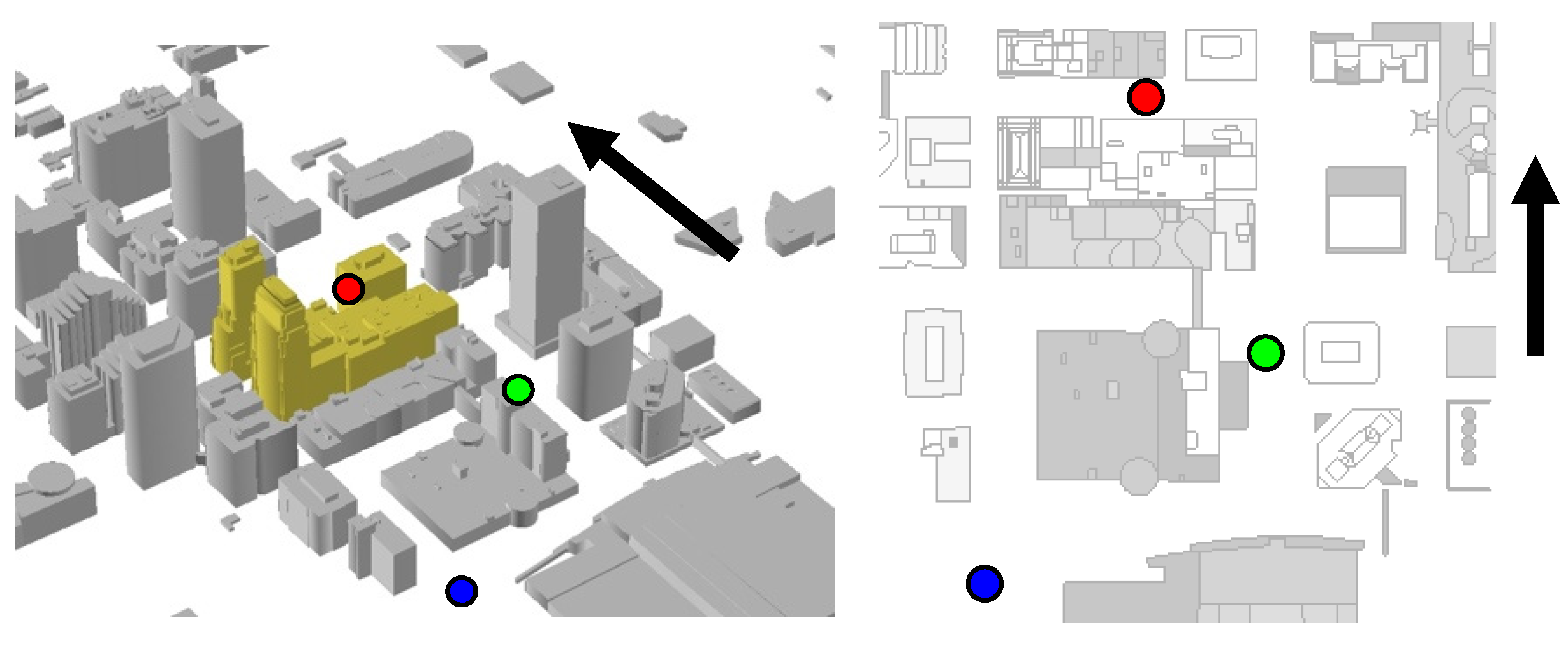
Aeolus results were compared to field data from a continuous release of sulfur hexafluoride (SF
6) during IOP 8 trial 2. As noted previously, the winds were predominantly from the south for this release. The event was chosen because there was little variation in the inflow wind direction and the edge of the plume was well captured by the gas sampler data. The portable wind detector at the city post office (PWID 15), a propeller anemometer, was used to record the ‘wake-free’ inflow profile for wind direction and wind speed. It was located about 500 m upstream of the central business district at 50 m above ground on a 35 m rooftop tower, and was free from building effects. A total of 5488 g of SF
6 gas was released continuously for 30 min from the Westin location shown in
Figure 6.
The computational domain is displayed in
Figure 1 (left) and was 1.2 km × 1.4 km × 0.21 km in the
x,
y, and
z directions discretized on a regular grid (Δ
x = Δ
y = 5 m, Δ
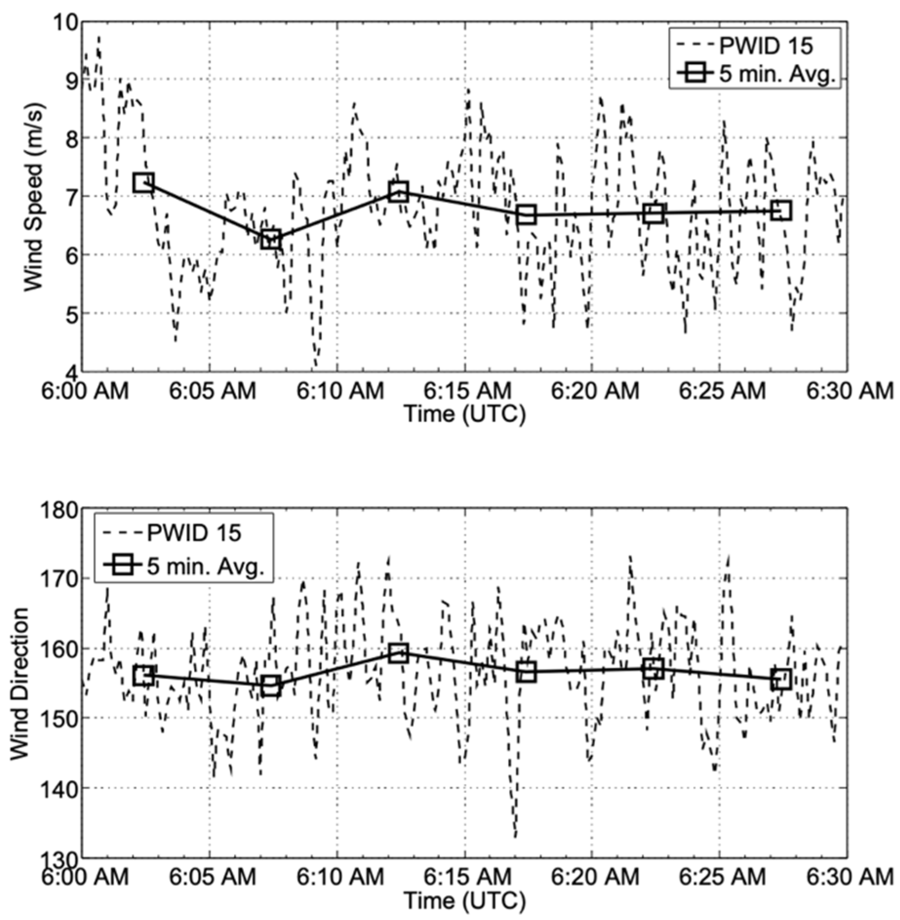
z = 3 m). The horizontal grid resolution of 5 m is the minimum grid spacing needed to resolve a typical street canyon. The grid consists of about 4.5 million cells. Time varying input for the simulation was constructed using data from the PWID 15 anemometer. Six log-law profiles using a surface roughness value of
z0 = 0.1 m (5 min average) were used in the LES simulation.
Figure 7 shows the wind speed and direction measured by the anemometer (dashed lines) and the five minute averaged values used to construct the Aeolus input wind profile (solid line, squares). The averaged log-law profiles were used to create the mean inflow profile while the inflow turbulence gerator perturbed the velcoity field to create physically realistic turbulent features. The source was defined as a sphere of 1 m radius and a release amount of 5488 g was simulated by releasing 0.5 million lagrangian particles over the release duration of 30 min. It was found that 0.5 million particels are sufficient to estimate 30 min averaged concentration at this spatial resolution.
Similarly to the complex terrain case, the flow field was simulated for 1.5 h, with the initial hour used for spinup and the final 30 min used for analysis and comparison with observations. The simulation took about 2 h of computer time to run on a quad-core machine.
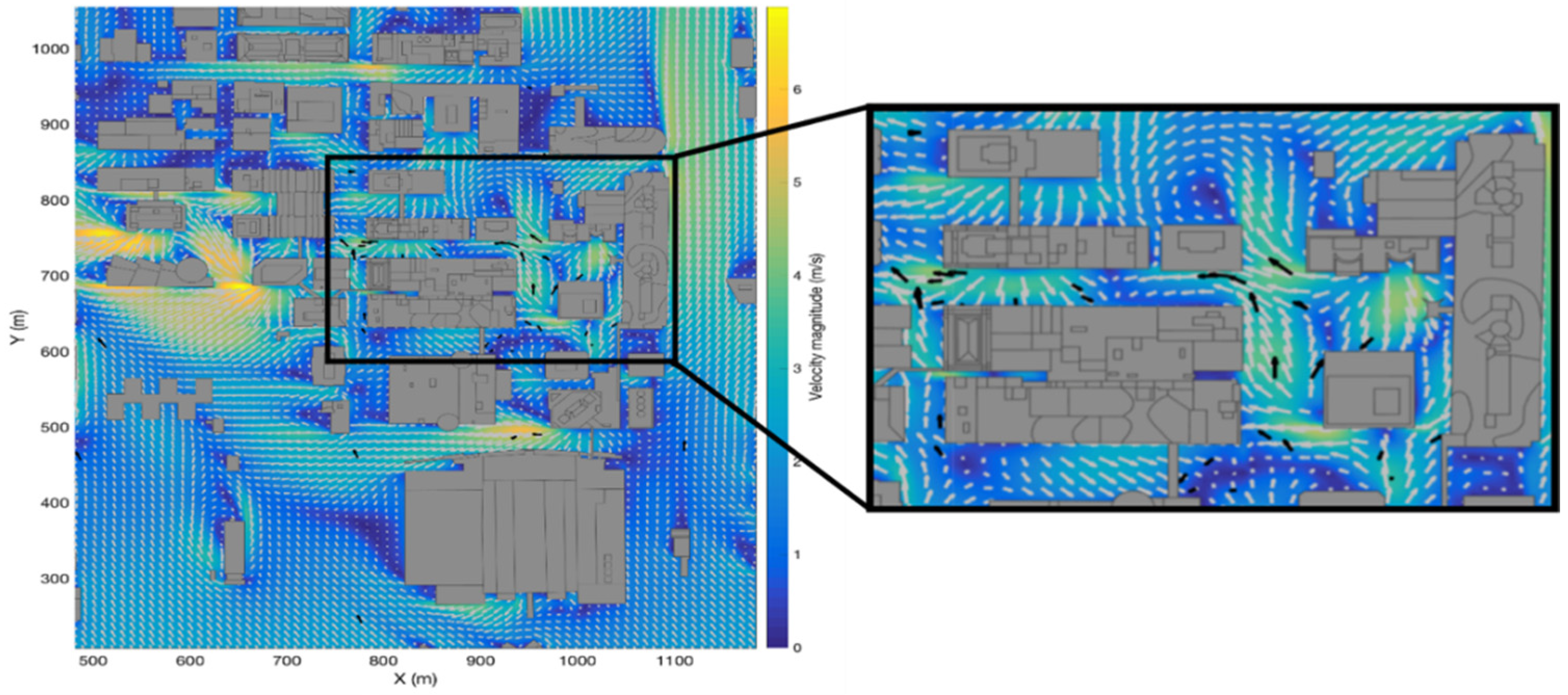
Figure 8 shows the velocity vector field for flow around Oklahoma City in the
x–
y plane at 8 m above ground level (AGL). Simulated wind vectors from the Aeolus model (grey arrows) are overlaid with meteorological observations (black arrows). Longer arrows in the figure indicate higher wind speed. The Aeolus wind speed prediction is also represented by the color shading around the buildings, where warmer colors indicate higher predicted wind speed values. From this figure, it can be observed that the Aeolus model is able to predict the important flow features reasonably well.
The model captures the channeling effects along north–south running streets and predicts the high wind speeds measured in these regions. Aeolus also predicts the reverse flow in the street canyons and wake regions in the domain. The model-produced velocities in the intersection areas are in good agreement with the field data.
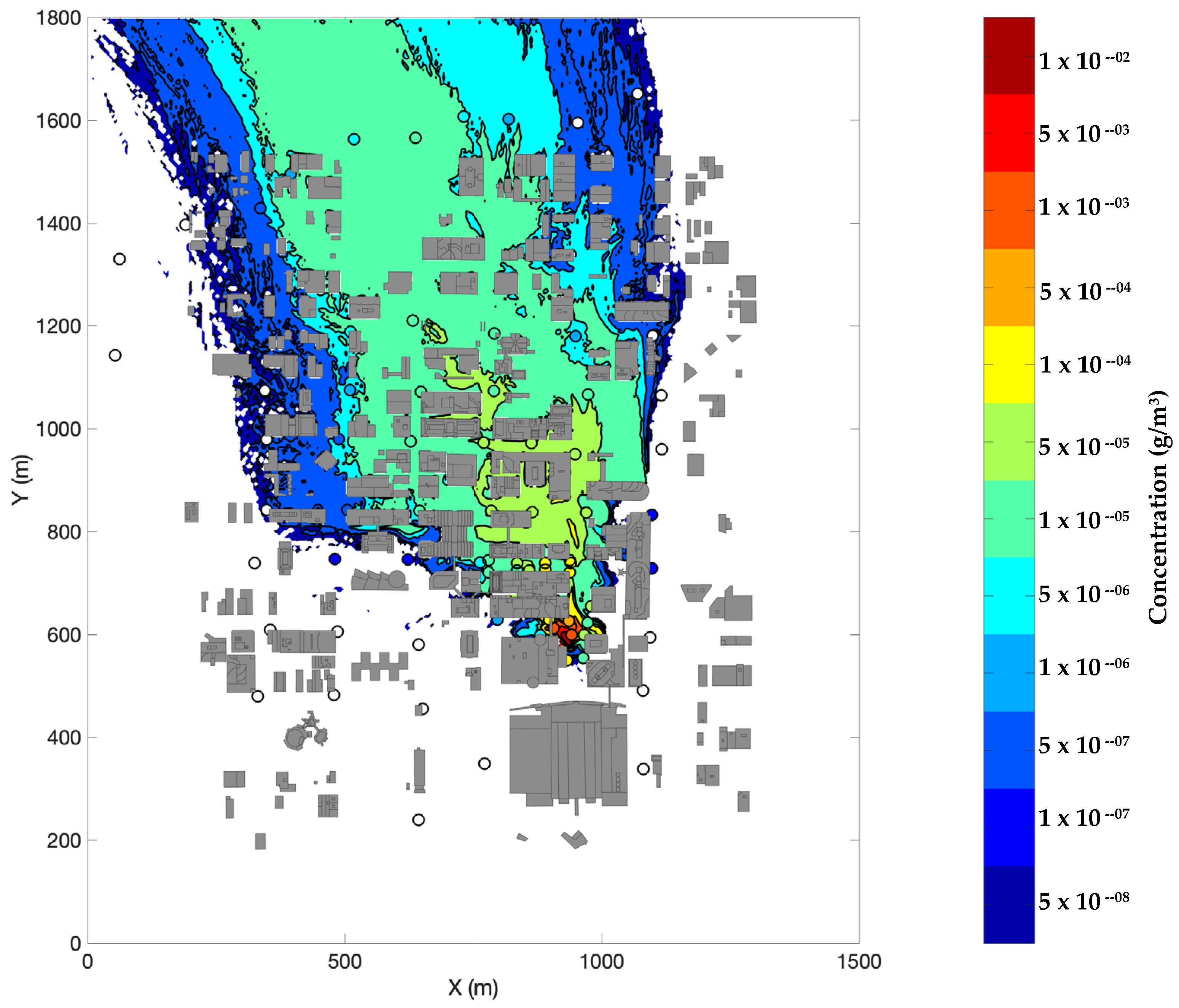
Figure 9 shows the measured and predicted SF
6 air concentration values at ground level. The colored circles represent the measured air concentrations averaged over the 30 min of the continuous release. The colored contours represent the Aeolus prediction of the 30 min average air concentration, with higher predicted values near the source (red, orange areas). The Aeolus model predictions agree with the experimental results well; the areas of highest concentration and the general downwind plume spreading are captured in the simulation results.
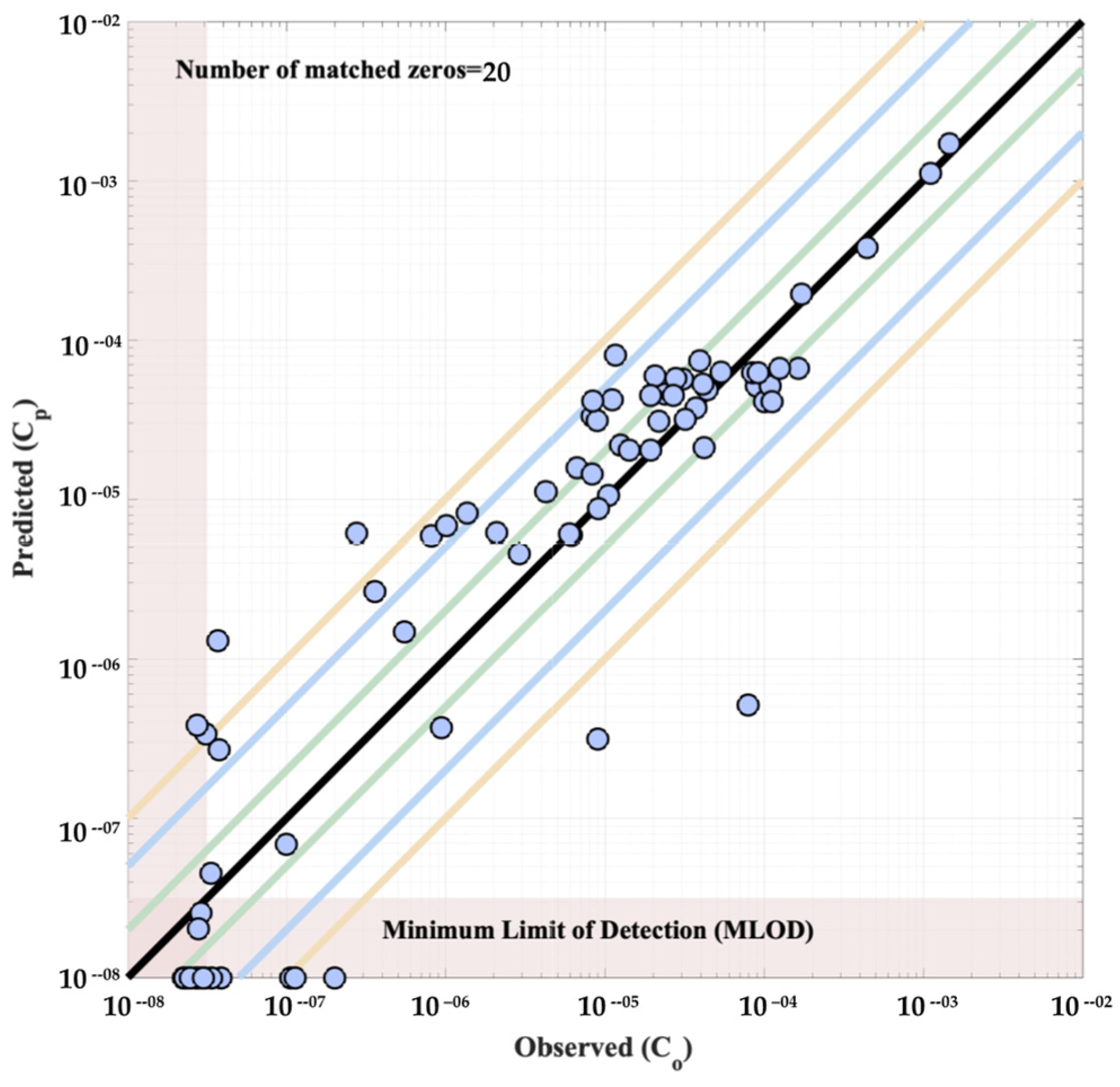
Figure 10 displays scatter plots of the paired (point-to-point) values from the Aeolus predictions and the field experiment measurements. Data points (blue circles) that fall on the solid black diagonal represent perfect matching between the predicted and measured values. Points that lie above and below the black line represent values that are over- and under-predicted by Aeolus, respectively, as compared to the measured data. The green, blue, and orange colored diagonal lines represent factors of 2, 5, and 10 model–measurement mismatches, respectively (FAC2, FAC5, and FAC10). The scatter plots show good agreement between predicted and measured values, with most pairs falling within the blue FAC5 lines.
Figure 10 also indicates that the number of matched zeros, which show how often the model correctly predicts zero-valued measurements (data below the instrument minimum level of detection, MLOD = 10
−7.5 g/m
3). The number of matched zeros shows that the model is able to correctly predict the spread of the plume. Overall, we found that 48.9%, 84.7%, and 91.5% of the simulated points fall within FAC2, FAC5, and FAC10, respectively, indicating excellent performance for predicting dispersion in complex urban areas which are consistent with the values suggested in Hanna and Chang (2012) [
25].
Further quantitative analysis of our results is given in terms of absolute value of fractional bias (|FB|) and the normalized mean square error (NMSE) for concentration. Fractional bias is a normalized value of mean error [
26]. |FB| values range from 0 to +2. A perfect agreement between model and measurement would result in FB = 0.
where
is the
ith observation (measurement), and
is the corresponding model prediction. NMSE captures the overall absolute departure of the modeled results from measurements. Lower values of NMSE indicate better agreement between model and experimental values.
where
n is the number of valid measurement–model data pairs and
is the mean measurement value. Hanna and Chang (2012) suggest the following limits on the comparison metrics for acceptable performance of an urban model [
25]:
|FB| ≲ 0.67, i.e., the relative mean bias less than a factor of ~2.
NMSE ≲ 6, i.e., the random scatter ≲ 2.4 times the mean.
FAC2 ≲ 0.30, i.e., 30% or more of model predicted values are within a factor of two of measured values.
The absolute value of the fractional bias (|FB|) was found to be 0.015 and the NMSE for the LES simulation was 0.29, indicating relatively low simulation errors compared to the experimental data. This excellent comparison of the Aeolus model with field measurements in complex urban areas makes it a very useful tool for predicting flow features and dispersion patterns in these scenarios.
5. High-Temperature Nuclear Cloud Rise Dynamics
For the final application, we ran Aeolus to simulate the dynamics of a hot nuclear detonation cloud rising in the troposphere with a specified ambient potential temperature profile θa. In this set-up, the source is not only a mass release, but also a large temperature perturbation. Therefore, the initialization requires the temperature, altitude, and size of the fireball formed from the detonation.
The Smagorinsky scheme in Aeolus (see
Section 2.1) is useful for simulating turbulence at standard atmospheric conditions, but not for including all the relevant turbulence scales in a buoyant nuclear cloud. Realistically, there is additional mass and energy exchange as ambient air is entrained into the cloud. In
Section 5.3, we describe a new parameterization that was added to Aeolus to represent this entrainment process.
5.1. Dixie Event Description
The Dixie test was performed during operation Upshot-Knothole on 6 April 1953 at 07:30 local time in Nevada (37°5′5″ N, 116°1′5″ W). The device was detonated in the atmosphere at 1.84 km AGL (3.1 km above mean sea level) with an explosive yield of 11 kilotons [
27]. These characteristics result in a scaled height of burst of 831 m corresponding to ‘regime 1’ in which no soil or dirt is disturbed due to the detonation [
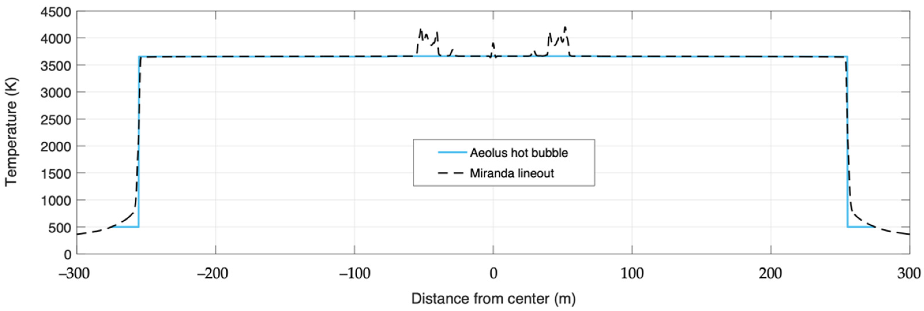
28]. During the shot, high-frequency cameras captured the formation and propagation of the shockwave and fireball for comparison with simulations, such as Miranda [
29]. Miranda simulates the initial fireball size and temperature, which is shown in
Figure 11 for the timestep directly before the Dixie cloud starts rising. Additionally, the time series of the observed top and bottom of the Dixie cloud were recorded in Hawthorne (1979) [
30].
Previous models successfully simulated Dixie cloud rise. Kanarska et al. (2009) compared predictions from a compressible Eulerian model with a low Mach number component [
31]. More recently, Arthur et al. (2021) used the Weather Research and Forecasting model to simulate Dixie cloud rise, finding good agreement with observations [
32]. However, neither of these prior modeling studies contained detonation gas and debris in the cloud, which is included in the Aeolus simulation.
5.2. Model Setup
In setting up the model grid, there is a tradeoff between having cells that are small enough to resolve the turbulent flow, but not too small because a large domain with many cells is required to simulate cloud rise throughout the troposphere. For this simulation, we selected a model resolution of Δx, Δy, Δz = 30 m in the x-, y-, and z-directions and a domain size of x, y, z = 9000 m, 9000 m, 15,000 m, resulting in 45 million grid cells.
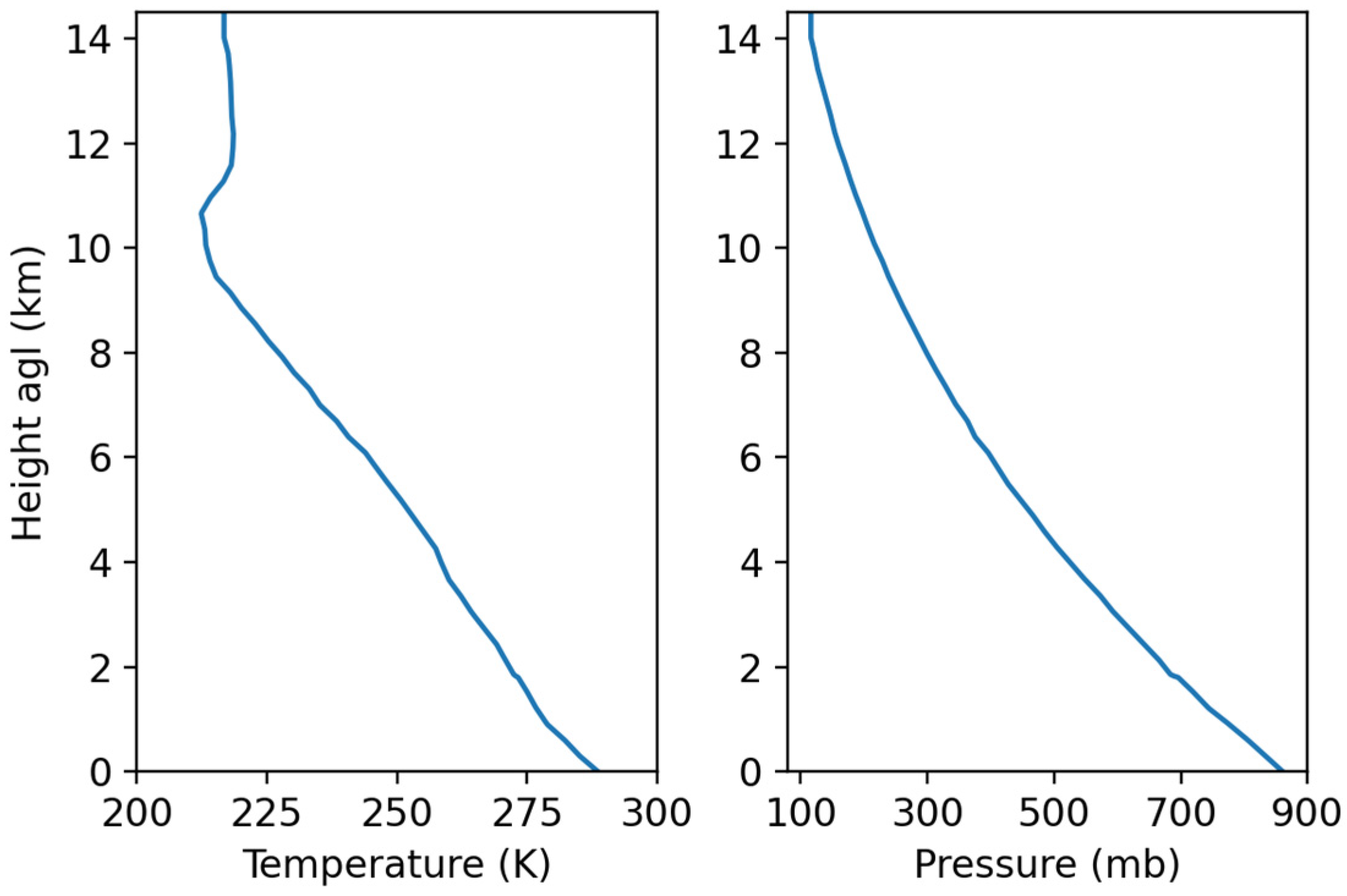
The ambient conditions are specified as vertical profiles of temperature and pressure at the detonation location. These input data are at a resolution of 304.8 m, and Aeolus linearly interpolates the temperature and pressure profiles to its vertical grid (
Tk,
Pk). The profiles utilized for the Dixie case from radiosonde measurements [
30] are shown in
Figure 12. The potential temperature of every grid cell
θi,j,k in Aeolus is set according to the vertical profile:
The source inputs defining the initial hot bubble include the detonation time , bubble diameter and temperature , the mass and number of Lagrangian particles representing materials in the hot bubble, the density and size of materials in the hot bubble, and the source position . Aeolus replaces the ambient potential tempertaure with the hot bubble potential temperature at the source location based on and the grid pressure at . Additionally, 1.8 million Lagrangian particles are released at random locations within the bubble volume, representing the hot cloud at .
5.3. Entrainment Parameterization
The momentum and energy balances are solved for the velocity and potential temperature fields at each grid cell center. Turbulent viscosity is determined based on the shear rate and Smagorinsky constant
Cs, but it is also enhanced by entrainment of ambient air that is not tracked in Aeolus. To account for the induced mixing from entrainment, we add an entrainment term (
) to eddy viscosity for momentum and potential temperature equation (
) at the grid cell at index
in the
x-,
y-, and
z-direction, respectively.
where
is contraction of the rate-of-strain tensor,
.
This enhancement due to entrainment is determined based on the vertical velocity of that cell
the potential temperature of that cell
, the ambient potential temperature at that vertical level
, and a dimensionless empirical parameter
entrainment factor.
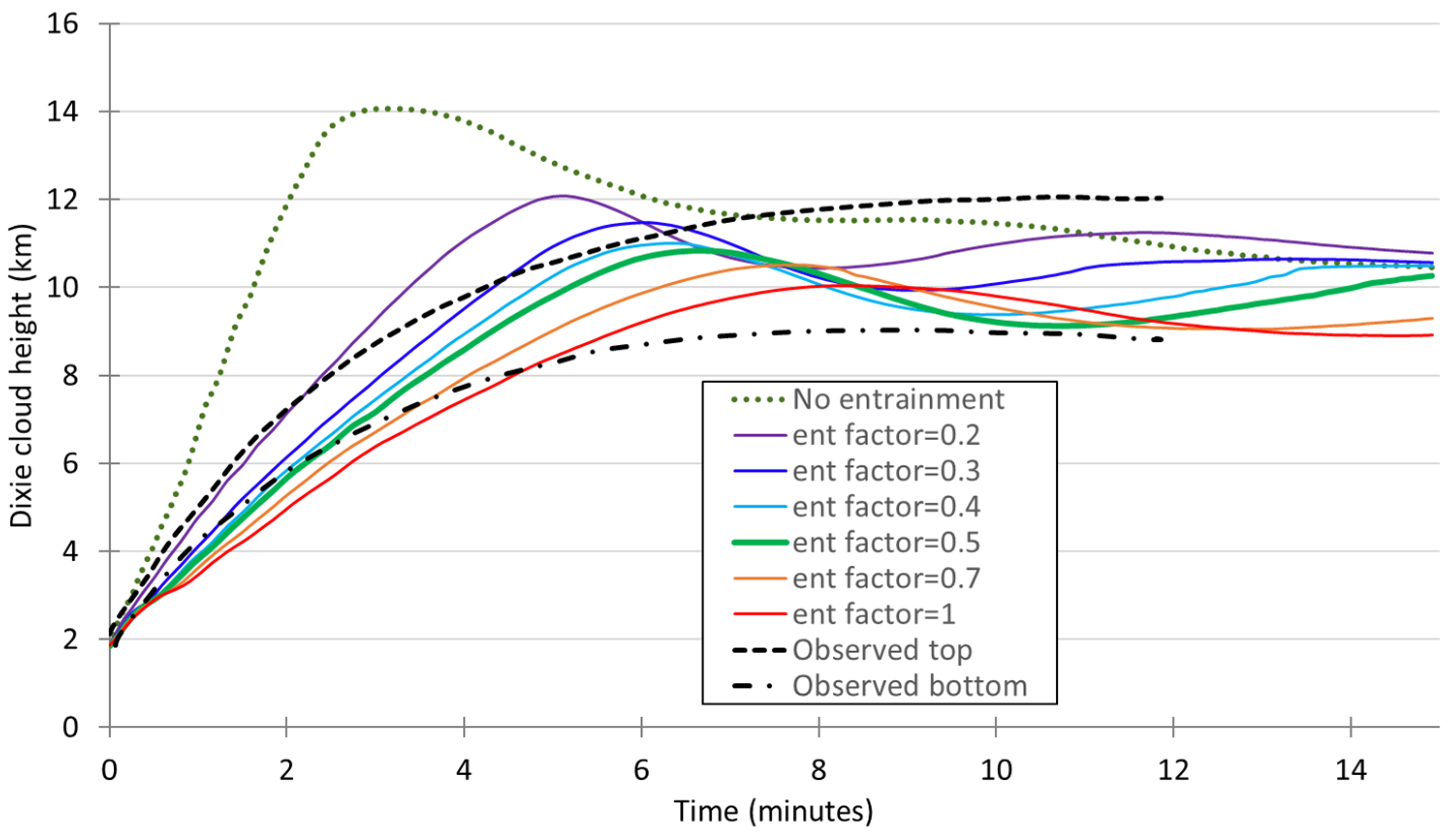
Using the model inputs and entrainment parameterization described above, we performed seven Aeolus simulations. The model set-up was identical for all seven simulations except that we varied
between zero and one. An entrainment factor of zero is equivalent to running a simulation without the entrainment parameterization. The results are shown in
Figure 13 where the green profile corresponding to
of 0.5 is the closest match to the observations.
The entrained ambient air slows the cloud rise velocity, decreasing the maximum cloud height. Additionally, entrainment results in oscillations around the stabilized cloud height since the cloud does not overshoot the tropopause height. The hot cloud rises above its neutral buoyancy height due to its inertia until the inertia cannot sustain the imbalance in density between the cloud and environment. At this point, the cloud is denser than its surroundings and it falls, carried past stabilization by its momentum. The oscillations continue as the cloud height converges to its stabilization height. Theoretically, the frequency of oscillations in a stratified environment can be described with the Brunt–Väisälä frequency
.
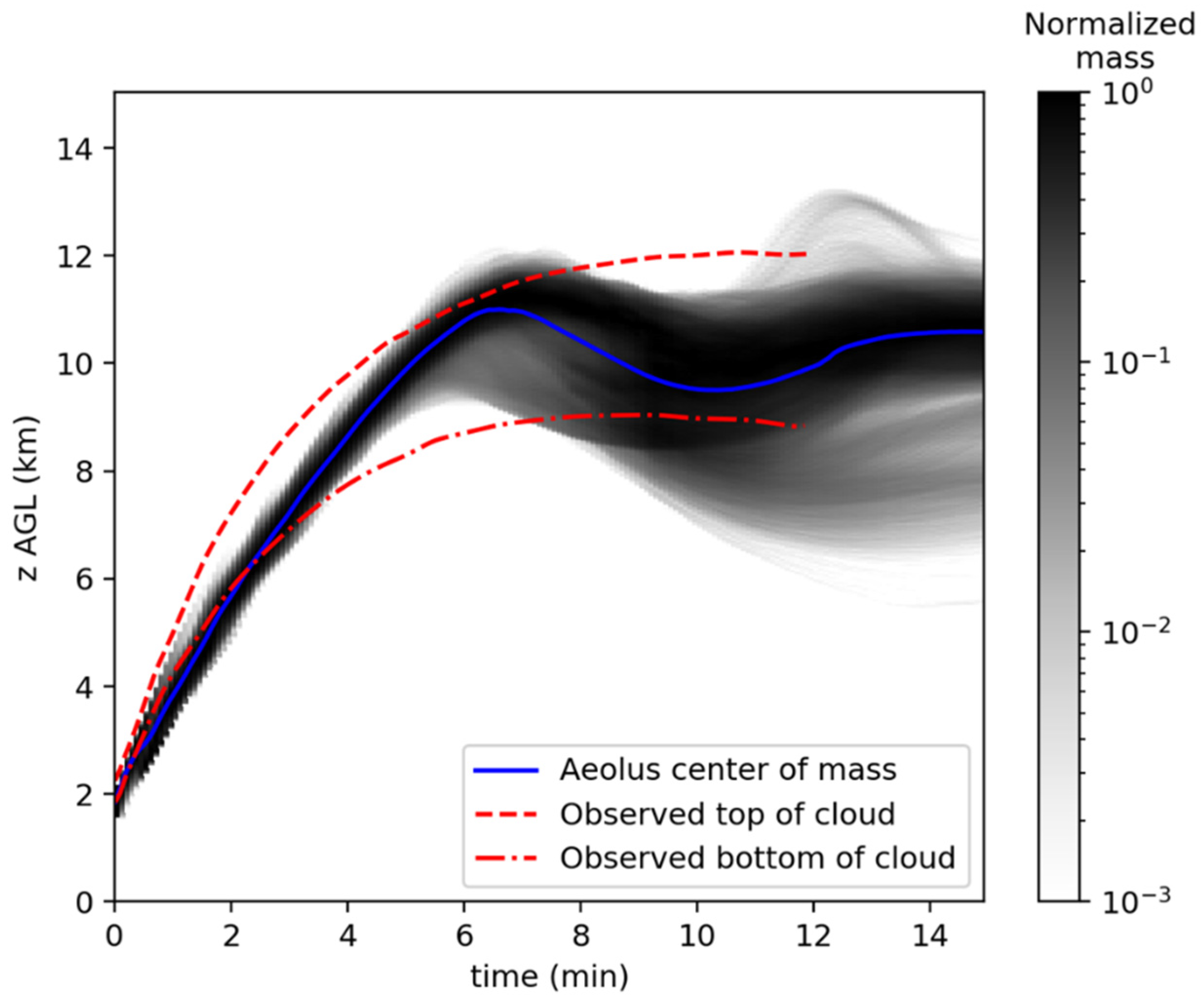
Figure 13 shows the cloud center of mass, which is not the best comparison to the observations of cloud top and bottom. Instead,
Figure 14 shows the normalized cloud mass (
) calculated from the average concentration in the
x- and
y-directions for each vertical level
(
) where
is the number of horizontal grid cells in each vertical level. The mean cloud mass is normalized so the maximum value of
is one, so the average concentration is divided by its maximum value across the vertical levels.
Similar to simulations by Arthur et al. (2021), the cloud height is underpredicted in the first 2 min post detonation [
32]. At later times, the majority of the cloud mass is contained between the observed cloud top and bottom, as shown in
Figure 14.
Figure 15 shows the evolution of the cloud temperature and gas and debris concentrations at 1.0, 3.5, 6.5, and 11.5 min after detonation. The potential temperature is shown across the
y- and
z-grid cells at
x = 4.5 km, which corresponds to the cloud center. The gas and debris concentrations are averaged over the x-direction and normalized by their respective source mass to determine their dilution ratios shown in
Figure 15. The cloud vertical extent, shown in the grey shaded area, is defined as the altitudes
in which the concentration is more than 10% of the current maximum concentration.
The cloud center is defined as the cloud center of mass within the cloud extent, which is shown as the black solid lines in
Figure 15.
The observed cloud top and bottom is also shown in
Figure 15 as the red dashed lines. The simulated cloud rise matches observations well on average, with an underestimate of the observed height initially and a slight overestimate at the maximum height near 6.5 min post-detonation. Additionally, even though the simulated cloud bottom extends lower than the observed after about 8 min (as shown in
Figure 14), most of the cloud below the observed bottom could be considered the stem instead of the cap.
6. Conclusions
Aeolus is a fast-running computational fluid dynamics urban dispersion model that has been validated using several experimental data sets. Using the Aeolus model, complex dispersal experiments can be completed with simulation run times small enough for use in emergency response, to provide consequence management information. The model is coupled to all the relevant databases required to setup and run the model and produce products which are useful for first responders.
In this work, we have simulated flow and dispersion using the large eddy simulation version of the Aeolus model in three different regimes—complex terrain, urban domain, and high-temperature cloud rising into high altitudes. This showcases the flexibility and adaptability of the model in different scenarios.
Comparing Aeolus predictions to field experiments, the model generally shows good agreement with the measured data. This report details model validation to the Askervein hill field campaign conducted in 1982 and 1983, the Joint Urban field experiments conducted in 2003 for both continuous and instantaneous tracer gas releases, and explosive cloud rise data from the Dixie nuclear test conducted at the Nevada Test Site in 1953. Aeolus results compare well with measured data both qualitatively and quantitatively and were found to compare well with the data.
Expanding the capabilities of a fast-running urban dispersion model and validating its simulation results against field data greatly advances NARAC’s ability to make predictions of the fate of material released in an urban environment and complex terrain. The improved and validated Aeolus model represents a significant capability for NARAC, and improved support to the USA’s Department of Energy.
In future, we plan to validate the LES model for additional complex terrain regions and other real and mock urban areas. We also plan on validating the model for different release types, including buoyant and dense gas releases in urban areas. Given the simplicity of the model to adapt to complex grids, we intend to extend the model for modeling flow and dispersion pattern in indoor environments. To further increase the efficiency of the large eddy simulation capability of the Aeolus model, we plan to implement the code on a Graphics Processing Unit (GPU) platform which will truly help in operationalizing the model.
In addition, we plan to validate the entrainment parameterization in nuclear cloud rise simulations using other test shots.


 ,
, 


