Article

Extreme Aerosol Events at Mesa Verde, Colorado: Implications for Air Quality Management

1
Department of Chemical and Environmental Engineering, The University of Arizona, Tucson, AZ 85721, USA
2
Department of Health Sciences, Northern Arizona University, Flagstaff, AZ 86011, USA
3
Department of Hydrology and Atmospheric Sciences, The University of Arizona, Tucson, AZ 85721, USA
*
Author to whom correspondence should be addressed.
Co-first authors.
Submission received: 16 August 2021 / Revised: 29 August 2021 / Accepted: 31 August 2021 / Published: 4 September 2021
(This article belongs to the Special Issue Air Quality Management)

Abstract

:
A significant concern for public health and visibility is airborne particulate matter, especially during extreme events. Of most relevance for health, air quality, and climate is the role of fine aerosol particles, specifically particulate matter with aerodynamic diameters less than or equal to 2.5 micrometers (PM2.5). The purpose of this study was to examine PM2.5 extreme events between 1989 and 2018 at Mesa Verde, Colorado using Interagency Monitoring of Protected Visual Environments (IMPROVE) monitoring data. Extreme events were identified as those with PM2.5 on a given day exceeding the 90th percentile value for that given month. We examine the weekly, monthly, and interannual trends in the number of extreme events at Mesa Verde, in addition to identifying the sources of the extreme events with the aid of the Navy Aerosol Analysis and Prediction (NAAPS) aerosol model. Four sources were used in the classification scheme: Asian dust, non-Asian dust, smoke, and “other”. Our results show that extreme PM2.5 events in the spring are driven mostly by the dust categories, whereas summertime events are influenced largely by smoke. The colder winter months have more influence from “other” sources that are thought to be largely anthropogenic in nature. No weekly cycle was observed for the number of events due to each source; however, interannual analysis shows that the relative amount of dust and smoke events compared to “other” events have increased in the last decade, especially smoke since 2008. The results of this work indicate that, to minimize and mitigate the effects of extreme PM2.5 events in the southwestern Colorado area, it is important to focus mainly on smoke and dust forecasting in the spring and summer months. Wintertime extreme events may be easier to regulate as they derive more from anthropogenic pollutants accumulating in shallow boundary layers in stagnant conditions.

1. Introduction

Particulate matter (PM) is a leading cause of death globally among environmental threats and was the fifth-ranking mortality risk factor as of 2015 [1], accounting for over 7 million deaths per year (~4.2 million from outdoor pollution) according to the World Health Organization [2]. In addition, atmospheric aerosol particles degrade visibility and air quality and have important impacts on climate and the hydrological cycle. Of concern are rare events when PM levels are extremely high, which can lead to an abrupt increase in risk for living beings and the environment. A region especially vulnerable to such events is the southwestern United States (U.S.), which is exposed to dust and smoke, in addition to various forms of anthropogenic pollution. In particular, wildfires are of growing concern owing to warming temperatures, and historic land management practices that yielded conditions conducive to larger and more frequent fires over the western U.S. [3,4,5]. Recent decades have coincided with rapid population growth, land use change, and increasing water shortages and drought, resulting in perturbations in aerosol emissions and their eventual effects (e.g., health, cloud formation, visibility, climate) on the region [6,7,8,9,10,11]. Seasonal characteristics of aerosol composition and concentrations have been discussed thoroughly in many past studies for the southwestern U.S. [12,13,14,15,16]. Of note is that the southwestern U.S. has the highest fine soil levels in ambient particles as compared to the rest of the country [17]. Furthermore, regulatory activities have been linked to reductions over time over the western U.S. for anthropogenic pollutants such as sulfate [18].
Mesa Verde National Park (NP) in southwest Colorado, near the four-corners area between Arizona, New Mexico, Utah, and Colorado (Figure 1), is located in an area where several sources of PM combine to lead to extreme PM events. Such sources include biomass burning, dust, natural biogenic and anthropogenic sources, and also long-range transport from other regions [12,13,17,19,20,21]. There are relatively small populated centers (population < 50,000) within a ~50 km radius, but there are major coal-fired power stations including the San Juan Generating Station and Four Corners Power Plant about 46 km and 53 km south of Mesa Verde NP, respectively (Figure 1) [22]. Knowledge of the frequency, intensity, and chemical characteristics of extreme PM events is helpful for developing strategies to mitigate their negative impacts. As fossil fuel combustion can be more easily controlled than natural aerosol sources (e.g., dust, smoke) [23], a potential concern for this region is if dust and smoke air quality events are more prevalent than those linked to anthropogenic emissions. Motivating this issue is that another study focused on the southwestern U.S. reported a decline in the number of extreme aerosol events based on criteria involving elemental carbon (i.e., anthropogenic pollutant) between 2001 and 2014 [24]. This study aims to use three decades of surface monitoring data at Mesa Verde, coupled to global aerosol model results, to address the temporal frequency of extreme PM events (monthly, day of week, interannual), categorization of such events into source categories, and the aerosol chemical characteristics of these events as a function of source category.

2. Methods

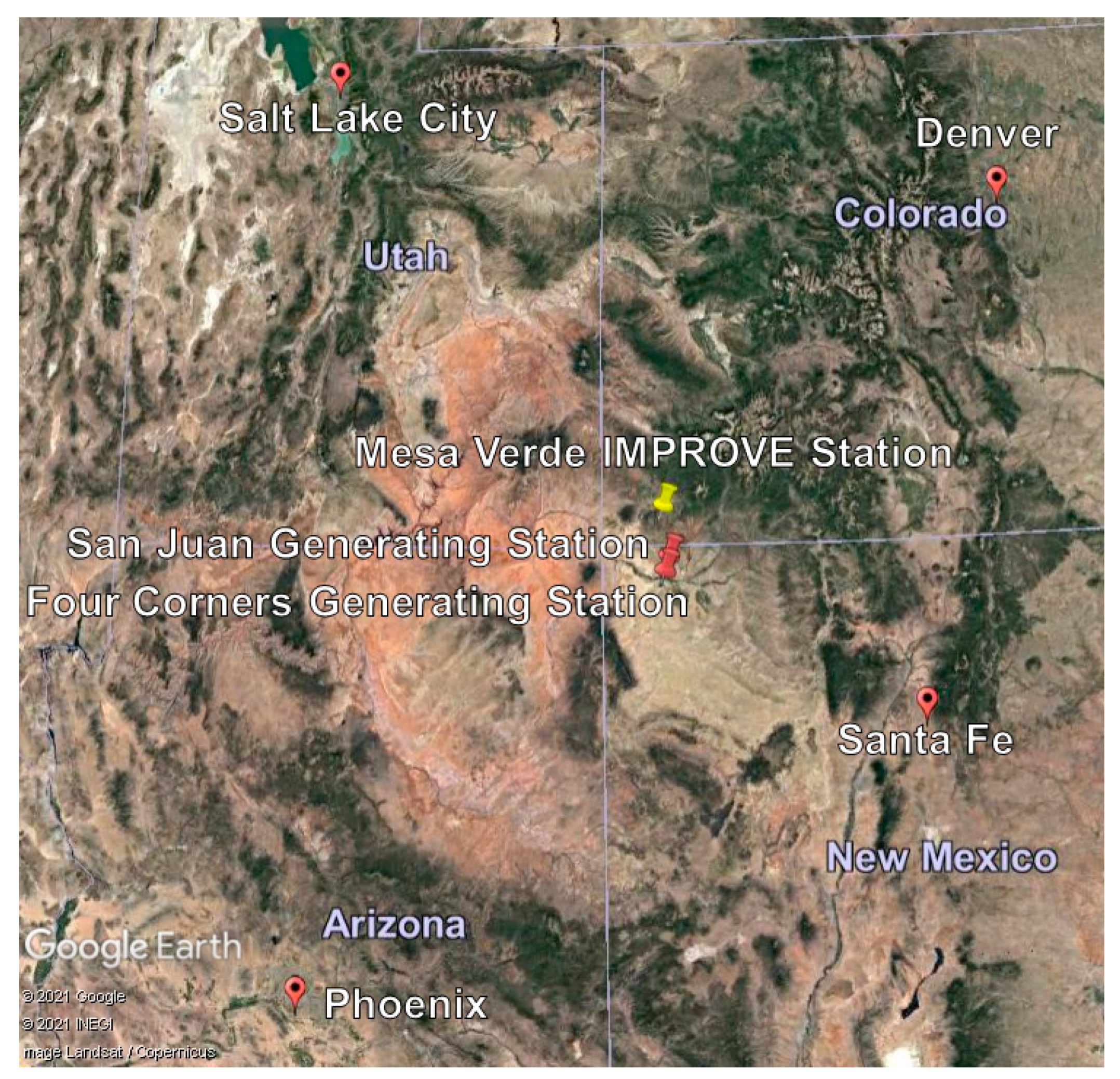
2.1. IMPROVE Site and Data Description

The Mesa Verde National Park (NP) Interagency Monitoring of Protected Visual Environments (IMPROVE) site (37.1984° N, 108.4907° W) in southwestern Colorado (Figure 1) is based in Montezuma County and at 2172 m above sea level (ASL). Other notable regional cities are shown in Figure 1, including Santa Fe, New Mexico (~295 km away), Phoenix, Arizona (~540 km away), Denver, Colorado (~405 km away), and Salt Lake City, Utah (~490 km away). This IMPROVE site collects 24 h filter samples throughout the week, with two collected per week (Wednesday and Saturday) before 2000, and one every third day after 2000. This shift in sampling schedule is not expected to bias the results shown in this study as the day-of-week analysis is only conducted for the period starting in 2000. Sampling details and protocols are explained in detail elsewhere (http://vista.cira.colostate.edu/improve/Publications/SOPs/UCDavis_SOPs/IMPROVE_SOPs.htm (accessed on 23 May 2021)), with numerous studies summarizing IMPROVE data details (e.g., [13,25]). Data are used for total mass concentrations of PM with aerodynamic diameters less than or equal to 2.5 µm (PM2.5) and 10 µm (PM10), as measured gravimetrically. Speciated data are used from the PM2.5 samples, with water-soluble ions (e.g., SO42−, NO3) detected via ion chromatography, elements from sodium (Na) to manganese (Mn) measured with particle-induced X-ray emission (PIXE), and elements ranging from iron (Fe) to lead (Pb) detected with X-ray fluorescence (XRF). Organic carbon (OC) and elemental carbon (EC) were measured with a thermal optical reflectance method of carbon analysis [26,27]. We report IMPROVE concentrations for fine soil in the PM2.5 fraction, which are calculated using this equation [25], supported by earlier analysis of local soils and ambient aerosol particles [28,29]:
Fine Soil (µg m−3) = 2.2[Al] + 2.49[Si] + 1.63[Ca] + 2.42[Fe] + 1.94[Ti]
The criteria used here to define extreme events hinges on calculating the 90th percentile value of PM2.5 for each month based on data for the full-time duration of this study, and assigning any day with a PM2.5 level above that threshold as an extreme event. A similar strategy has been used in other studies of this nature for parts of the southwestern U.S. [24].

2.2. Meteorological Data and Calculations

A series of datasets were collected from 1 January 2014 through to 31 December 2018 co-located with the Mesa Verde NP IMPROVE site and are briefly described here. The maximum and minimum temperatures were retrieved via the University of Utah’s MesoWest database [30,31,32]. The closest station to the park was Cortez-Montezuma County Airport (KCEZ; 37.3031° N, 108.6281° W) at an elevation of 1799 m ASL. Average temperature data were retrieved from the Western Regional Climate Center (WRCC; station COOP) [33]. Precipitation accumulation data were retrieved from the National Atmospheric Deposition Program (NADP) site at the Mesa Verde NP-Chapin Mesa site (CO99; 37.1979° N, 108.4910° W at 2162 m ASL) [34]. Cloud fraction data were retrieved from the moderate resolution imaging spectroradiometer (MODIS)-Aqua platform at 1° spatial resolution. Planetary boundary layer height (PBLH) data were retrieved from Modern-Era Retrospective analysis for Research and Applications-Version 2 (MERRA-2) at a spatial resolution of 0.5° × 0.625° [35]. Data for specific humidity and soil moisture at a depth of 0–10 cm at a spatial resolution of 0.25° were obtained from the Global Land Data Assimilation System (GLDAS) [36]. Data for the aforementioned four parameters (cloud fraction, PBLH, specific humidity, and soil moisture) were downloaded from NASA GIOVANNI [37]. Wind speed data were retrieved from Environmental Protection Agency (EPA) Air Quality Monitors associated with the EPA Air Quality System (AQS) at the Mesa Verde NP Resource Management Area IMPROVE station [38].
MesoWest reported maximum and minimum daily temperature values for each year examined. The average maximum and minimum temperatures were calculated for each month of a given year, and then the average of each month was taken for both temperature parameters across all five years (2014–2018). WRCC reported the monthly average of average daily temperatures at the chosen site starting in 1922, which were used to calculate the average monthly temperature within the time period. The total amount of precipitation measured via a rain gauge per month at the CO99 site was reported for each year after April 1981. The average amount of precipitation for each month during the 2014–2018 period was calculated from the given values. Cloud fraction, PBLH, specific humidity, and soil moisture content were reported as monthly means for the given time period, and the average for each month was calculated across all five years. Daily average wind speed values were averaged for each month of the year and then the average of each month was taken across all five years.

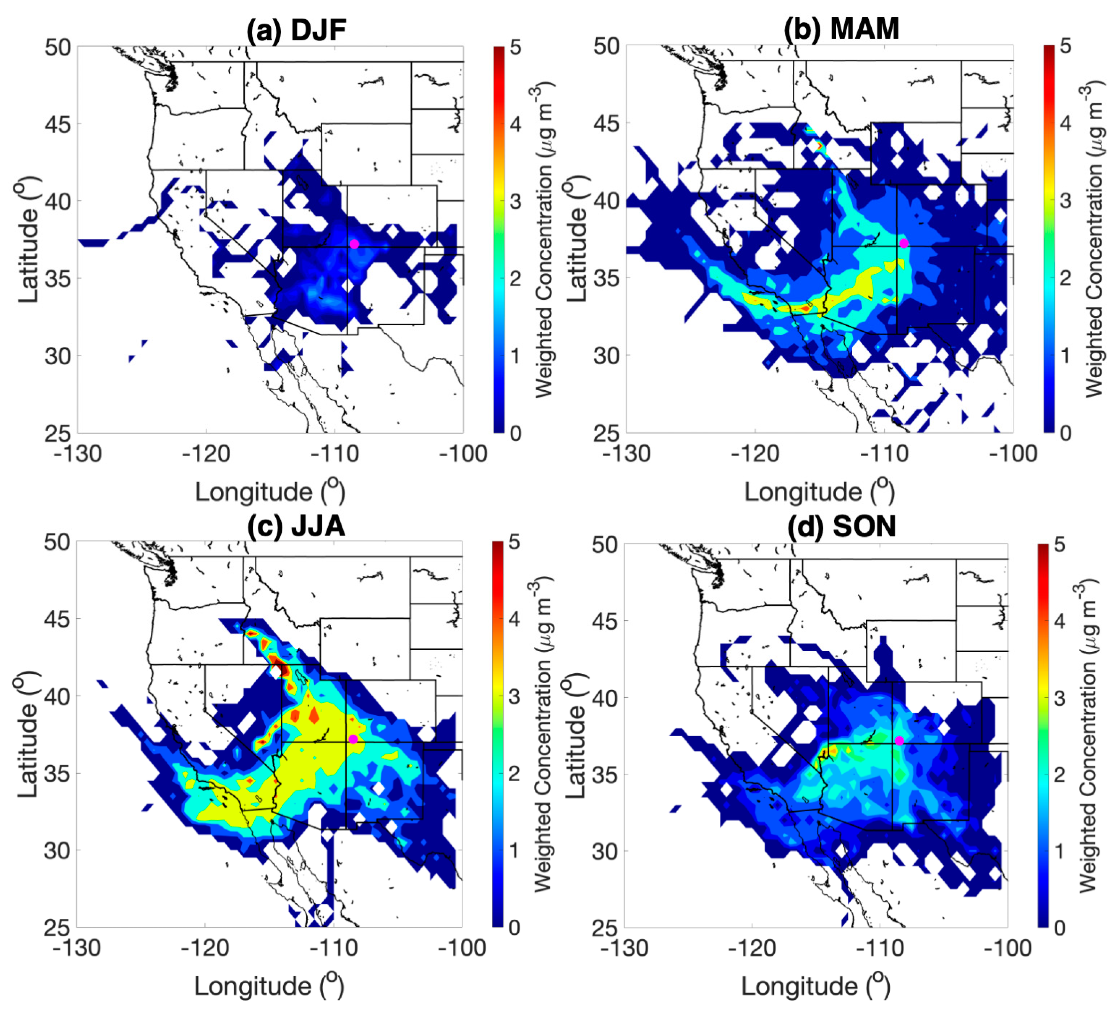
2.3. Trajectory Modeling

The NOAA Hybrid Single-Particle Lagrangian Integrated Trajectory (HYSPLIT) model [39,40] was used to obtain air mass back-trajectory information. We used the Global Data Assimilation System (GDAS) for simulations at 0.5° × 0.5° spatial resolution along with the “model vertical velocity method” to drive vertical transport. We used the ending point at the IMPROVE station for simulations and a 0.5 km ending altitude as that level has been used successfully in several other studies examining surface layer air quality [41,42,43].
We also used concentration weighted trajectory (CWT) analysis to gain insight into the predominant source regions and transport corridors for elevated PM2.5 levels at Mesa Verde for different seasons. A weighted concentration is applied to HYSPLIT grids derived from measured concentrations linked to individual 96 h back-trajectories passing each grid. This method is described in more detail in the literature [44,45,46,47,48]. The TrajStat software package (GIS-based) was used to develop CWT profiles [49]. CWT analysis was conducted using the most recent five years of the study period as this duration was deemed representative of general conditions for the entire 30 year period.

2.4. NAAPS and Air Mass Type Assignments

For determining whether smoke or dust contributed to individual extreme event days, we rely on the Navy Aerosol Analysis and Prediction System (NAAPS) [50], which is summarized at https://www.nrlmry.navy.mil/aerosol/ (accessed on 18 June 2021). The model has 25 vertical levels and provides data every 6 h at 1° × 1° spatial resolution. The Navy Global Environmental Model (NAVGEM) [51] provides meteorological data to drive NAAPS. We specifically used data for optical depths and surface mass concentrations associated with dust, smoke, and sulfate in this work for assigning extreme events to specific sources. We use the NAAPS results to classify extreme PM2.5 events into the following categories: (i) “Asian dust” if elevated dust optical depths extend from Mesa Verde to East Asia; (ii) “non-Asian dust” if there are high dust optical depths and surface mass concentrations regionally but not extended towards East Asia; (iii) “smoke” if there are enhanced smoke optical depths and surface mass concentrations regionally; and (iv) “other” if there were not enhanced dust or smoke optical depths or surface mass concentrations regionally. It is cautioned that NAAPS data were used starting in March 1998, and thus the air type classifications do not extend across the entire time range of analysis starting in 1989.

3. Results and Discussion

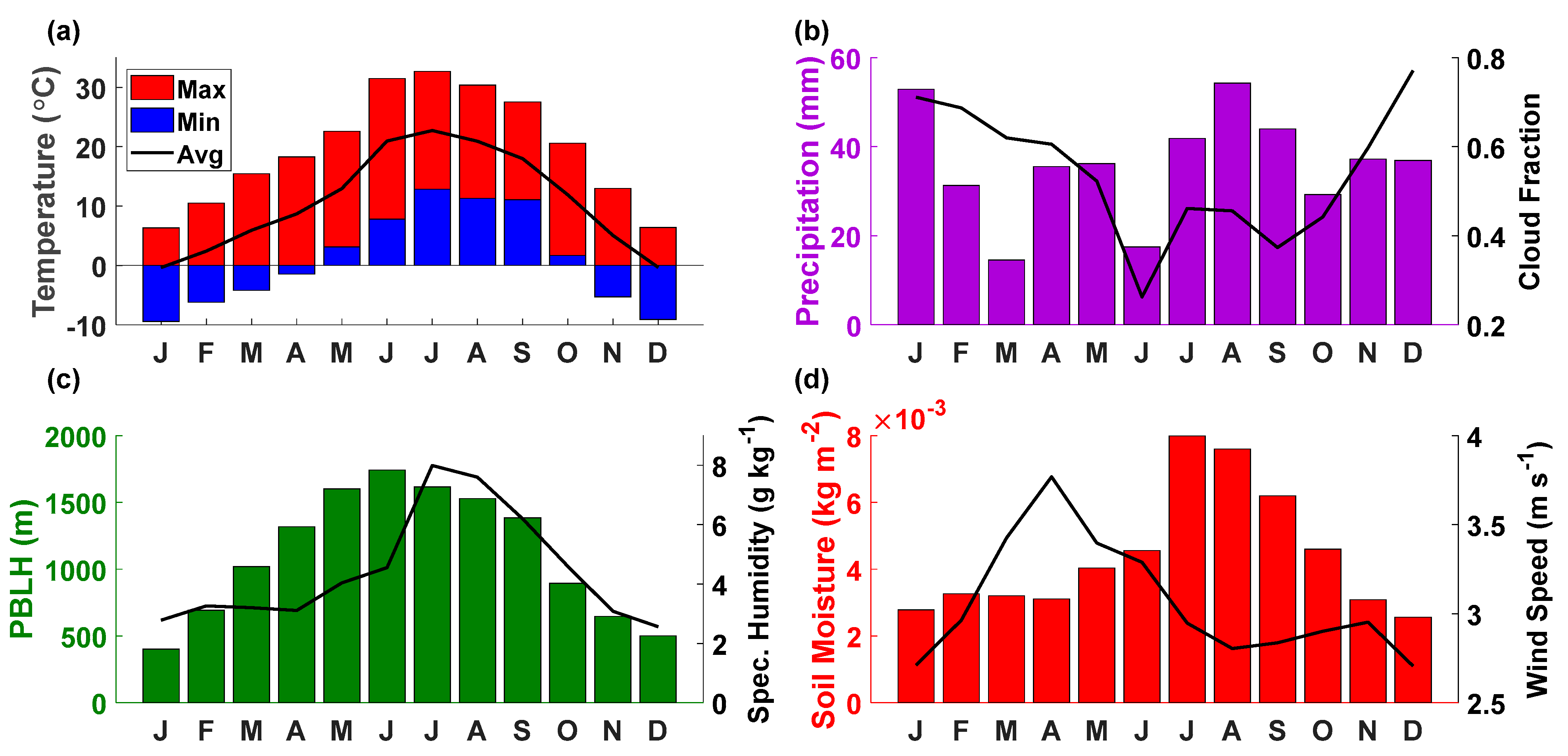
3.1. Meteorological Profile
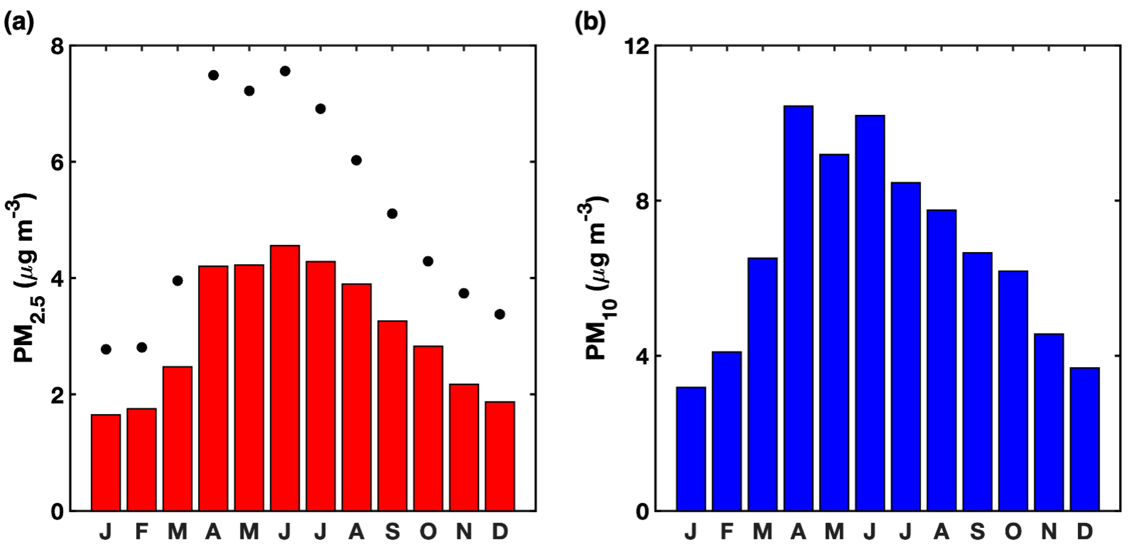
Meteorological data are first analyzed to provide environmental context for the study region (Figure 2). Hereafter we use the following seasonal acronyms: December–February (DJF), March–May (MAM), June–August (JJA), September–November (SON). The summer months (JJA) had the hottest temperatures with maximum levels exceeding 30 °C while the winter (DJF) and spring (March–April) months had a consistent minimum temperature below 0 °C (Figure 2a). The average temperature for the period of meteorological analysis (Jan 2014–Dec 2018) was 10.73 °C, with an overall maximum of 32.68 °C and minimum of −9.45 °C. The majority of precipitation occurred in the summer months (July–August) and the fall month of September, followed by a heavy precipitation period in late fall/early-mid winter (November–January) (Figure 2b). Maximum precipitation occurred during August with an average of 54.25 mm, while the minimum amount occurred during March averaging 14.53 mm (Figure 2b). The general trend for the cloud fraction included higher values in January (0.71) followed by a decrease until the end of June (0.26), with a mostly-gradual increase to December (0.77; Figure 2b). PBLH exhibited a trend following temperature with the lowest values in winter and reaching maximum heights in summer, peaking at 1742 m in June (Figure 2c). Specific humidity followed a similar trend to temperature, with a maximum humidity of 7.99 g kg−1 in July (Figure 2c). Wind speed had a peak during April (3.77 m s−1) with a mostly downward trend through the end of the year (Figure 2d). Soil moisture exhibited its highest values in the summer with a peak in July (7.99 × 10⁻³ kg m−2) (Figure 2d).

3.2. PM Profile

Monthly mean values of PM2.5 and PM10 are summarized in Figure 3, in addition to the 90th percentile values of PM2.5 per month (Figure 3a) that are used as the threshold concentrations above which PM2.5 values qualify as an extreme event in this study. PM2.5 levels exhibited peak monthly mean levels between April and August (3.9–4.6 µg m−3) and lowest levels in DJF (1.7–1.9 µg m−3). The 90th percentile values of PM2.5 expectedly followed the same monthly cycle as monthly mean PM2.5 levels ranging from as low as 2.8–3.4 µg m−3 in DJF to as high as 6.0–7.6 µg m−3 between April and August. The higher levels of PM2.5 in the spring and summer months are coincident with the months with the most dust and wildfire activity [9,20,52,53], in addition to high incident solar radiation and moisture that help promote secondary aerosol formation [19,54].
Monthly mean PM10 values ranged from lower values in DJF (3.2–4.1 µg m−3) to peak values between August and July (9.2–10.4 µg m−3). The difference between PM2.5 and PM10 is presumed to be largely due to dust particles in this region [9,20,22]. The highest PM10:PM2.5 ratios based on monthly mean concentrations occur in March (2.6) and April (2.5), which is presumed to be a marker indicative of high local dust influence [55].
Seasonal concentrated weighted trajectories from the most recent five years of the study period (December 2013–November 2018) (Figure 4) were used to provide further insight on influential transport corridors leading to high PM2.5 at Mesa Verde NP. The high mass concentrations during the summer (JJA) are largely associated with trajectories from the southwest and northwest. The next highest mass concentrations during the spring months (MAM) are linked to similar transport behavior as JJA albeit with reduced PM2.5 concentrations. A subtle difference between MAM and JJA is that the latter has more ‘hot spots’ of influential PM2.5 to the northwest, possibly from biomass burning owing partly to dry and hot conditions (Figure 2a), whereas the former has more influence from the southwest direction likely from dust owing partly to high winds and low soil moisture (Figure 2c,d). Subsequent extreme event source analysis for each season (Section 3.3) will support these speculations. The CWT map for MAM shows the widest reach in terms of how far away areas impacted PM2.5 at Mesa Verde, consistent with high surface wind speeds (Figure 2) and well-documented influence from long-range transport in this season from as far upwind as East Asia [56]. The SON and DJF seasons had lower PM2.5 and the DJF was particularly unique in terms of having the narrowest spatial range of influential source regions. This is due largely to the colder months having more stagnant conditions, as demonstrated by low surface wind speeds (Figure 2d) and shallow boundary layer heights (Figure 2c).

3.3. Demonstration of Extreme PM2.5 Events

We next demonstrate case examples of each source type contributing to extreme PM2.5 events at Mesa Verde NP before examining temporal trends. The first event shown (Figure 5) on 5 April 2010 was classified as an Asian dust event based on NAAPS and HYSPLIT results. NAAPS data going as far back as 24 March 2010 show significant dust optical depths over northeastern Asia that persisted along their journey across the Pacific Ocean towards the Mesa Verde area. Areas with higher dust surface concentrations coincided with areas with higher dust optical depth. On the day of the event, the following IMPROVE concentrations were measured, with the concentrations for species beginning with fine soil specific to the PM2.5 size fraction: PM2.5 = 34.5 µg m−3; PM10 = 186.8 µg m−3; fine soil = 41.2 µg m−3; Fe = 1.3 µg m−3; Al = 4.9 µg m−3; Ca = 1.5 µg m−3; K = 0.9 µg m−3; Si = 9.8 µg m−3. All of the aforementioned PM constituents are associated with Asian dust and each was pronounced in magnitude.
The second event shown from 16 April 2013 is a non-Asian dust case as it clearly demonstrates the lack of any extended dust optical depths from Mesa Verde NP towards Asia on the days preceding this event (Figure 6). The likely source of the dust was regional in nature (i.e., eastern Arizona) based on the HYSPLIT and NAAPS results. As dust events are most common in MAM for the study region, it is expected that the Asian and non-Asian events will typically reside in greatest number in the spring months. IMPROVE concentrations during this event day were as follows: PM2.5 = 40.3 µg m−3; PM10 = 98.2 µg m−3; fine soil = 27.6 µg m−3; Fe = 1.4 µg m−3; Al = 2.8 µg m−3; Ca = 1.5 µg m−3; K = 0.7 µg m−3; Si = 6.1 µg m−3.
The third event on 30 October 2003 was a smoke event marked by transport from southern California and Baja California (Figure 7). High smoke optical depth was observed in this region two days before the extreme smoke event was identified at Mesa Verde NP. High smoke surface concentrations can be seen stretching from southern California across the southwestern U.S. on the day of the event. IMPROVE measurements the day of the event support a smoke source based on enhancements in documented smoke tracer species [57,58,59]: PM2.5 = 32.5 µg m−3; PM10 = 117.7 µg m−3; fine soil = 12.0 µg m−3; OC = 8.7 µg m−3; EC = 0.9 µg m−3; K = 0.6 µg m−3; Ca = 0.8 µg m−3; SO42− = 0.7 µg m−3; NO3 = 1.4 µg m−3.
Finally, the fourth event on 9 January 2003 was classified as “other”, with transport from the Texas-Mexico border area (Figure 8). The likely sources contributing to this “other” event are anthropogenic in nature, and the high sulfate optical depths over western Texas support this notion. Sulfate was the only speciated optical depth recognized as enhanced by NAAPS for the region shown two days before the extreme event. NAAPS sulfate surface concentrations were elevated at Mesa Verde the day of the event because the sulfate-rich air mass was transported from western Texas to the Mesa Verde area. IMPROVE concentrations were as follows, with sulfate being notably enhanced: PM2.5 = 4.1 µg m−3; PM10 = 6.0 µg m−3; fine soil = 0.6 µg m−3; OC = 0.6 µg m−3; EC = 0.2 µg m−3; K < 0.1 µg m−3; Ca = 0.1 µg m−3; SO42− = 1.0 µg m−3. The DJF season is the season most likely to experience the most “other” events owing to stagnant conditions accumulation local and regional pollution, and also due to the lack of other extreme event sources that are more common in MAM and JJA such as dust and fires.

3.4. Monthly Profile of Extreme PM2.5 Events

The number of extreme PM2.5 days per month based on source category is summarized in Table 1 based on the criteria used from Section 2.1. “Other” sources were the most abundant relative to the other three categories for most of the annual cycle including between October and February. The “other” sources were especially influential compared to other sources in the colder winter months owing to limited dust and wildfires, in addition to stagnant conditions conducive to the build-up of local anthropogenic emissions (i.e., Figure 4).
Dust sources were most responsible for extreme events in March (40%), April (64%), and May (53%), whereas smoke was most important in June (67%), July (72%), August (83%), and September (53%). These results are in line with expectations for the following reasons. The predominant months linked to dust events, whether from Asia or regional sources, are in the springtime [9,56,60,61,62], whereas wildfires are active in the hot and dry summer months [59,63,64,65]. Asian dust was much more influential towards contributing to extreme PM2.5 events as compared to non-Asian dust between March and May owing likely in some part to the high altitude of this site being more receptive to long-range transported dust as compared to lower elevation sites such as in Arizona that have more influence from local sources [24].

3.5. Day of Week Profile of Extreme PM2.5 Events

Natural sources of aerosol particles (e.g., dust, sea salt) are not expected to follow a specific weekly cycle in contrast to anthropogenic sources that typically yield higher pollutant concentrations during the workweek and lower values during the weekend [66,67,68,69,70]. However, a concern in populated regions is anthropogenic dust (e.g., construction, recreational activity, resuspension from vehicular traffic) [71,72,73,74,75], which can follow a traditional weekly cycle with higher levels in the workweek similar to other traditional anthropogenic tracer species such as EC [57,66]. Although our analysis is not a typical weekly cycle analysis in that we are investigating selected events based on criteria of exceeding a monthly-specific 90th percentile of PM2.5 concentration, it is still of interest to examine the temporal profile of extreme PM2.5 events. This day of week analysis is shown in Table 2 and is limited to data beginning in 2000 when IMPROVE sampled every third day rather than only on Wednesday and Saturday in earlier years.
The days with most events across the entire study period were Friday and Saturday (30), with the other days having between 20 (Monday) and 29 (Thursday) extreme PM2.5 events. The two types of sources with the highest potential to have an anthropogenic signature include foremost “other” followed by non-Asian dust, assuming the latter had influence from anthropogenic dust emissions. The “other” category exhibited most of its events on Saturday (13), with the other days of the week having between 5 (Monday) and 12 (Sunday and Wednesday) events per day. Non-Asian dust events were most common on Friday (4 events), although there was a fairly small range between the days of the week (1–4 events per day of the week). The frequency of smoke events per day ranged from 7–15 per day, whereas Asian dust ranged from 2–5 per day. The day of week analysis does not point to any clear weekly cycle of when extreme PM2.5 events, which is a consequence partly of the appreciable contribution of non-anthropogenic forms of PM to these events. Furthermore, meteorological factors that do not typically exhibit weekly cycles are likely an interfering factor for when PM2.5 levels reach abnormally high levels in certain months [54]. Another study focused on extreme aerosol events across Arizona also did not observe any statistically significant differences for number of events on specific days of the week [24].

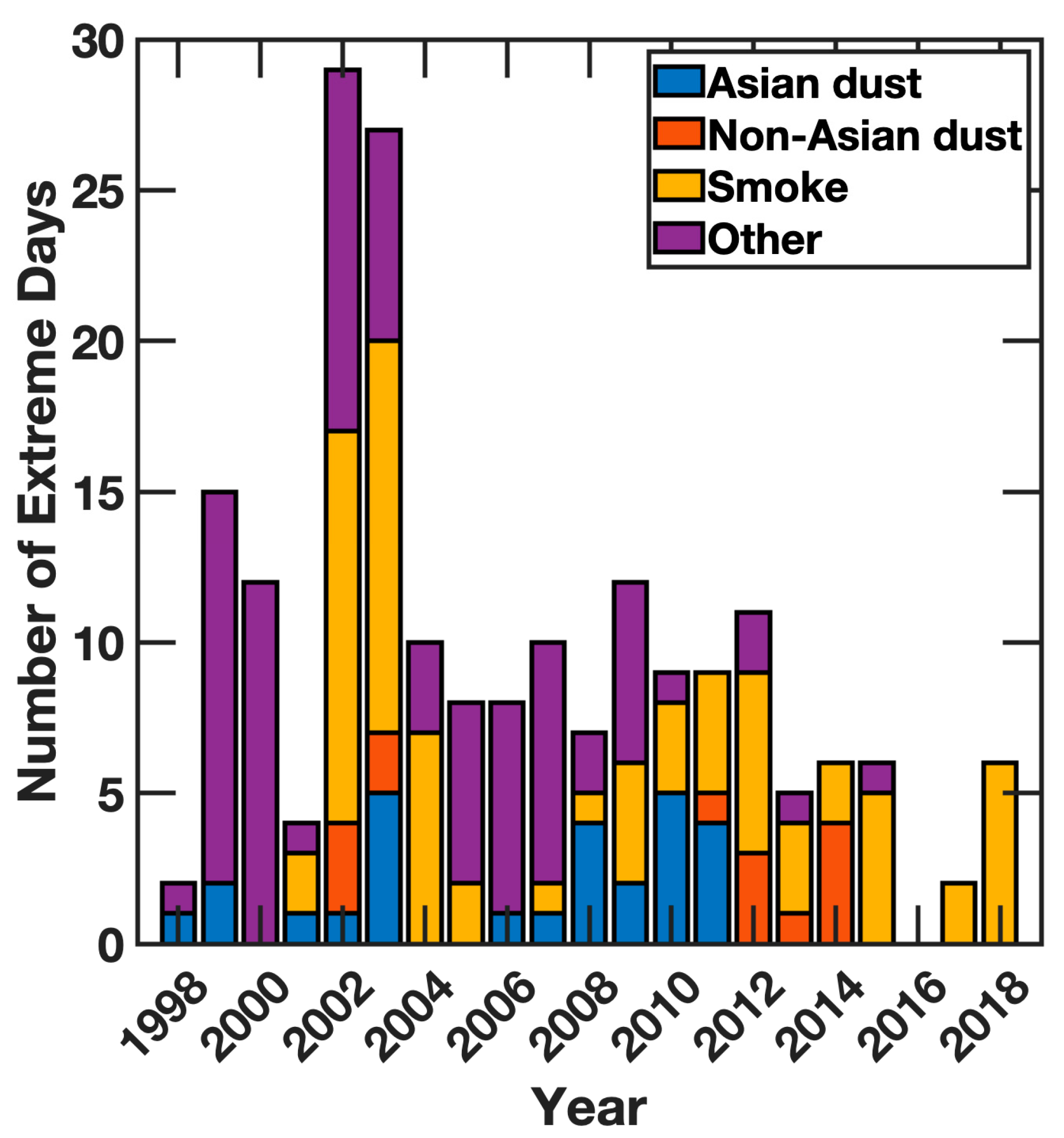
3.6. Interannual Profile of Extreme PM2.5 Events

Figure 9 shows the interannual frequency of extreme PM2.5 events, broken down into source categories with the caveat that 1998 had sparse NAAPS data across the full year. The years 2002 and 2003 had the most events (29 and 27, respectively), with the most common source being smoke (45% and 48% of events, respectively). The “other” category tended to contribute relatively more to extreme events up to 2008, after which the dust and smoke categories became relatively more influential. Smoke was the largest contributor in recent years (2012, 2013, 2015, 2017, 2018; 54–100% of events per those years).

3.7. Chemical Characteristics of Extreme PM2.5 Events

Average (±standard deviation) characteristics of total PM and speciated concentrations and selected chemical ratios are discussed next (Table 3) to parse out features specific to the individual sources identified with NAAPS. Both PM10 and PM2.5 were highest for the Asian dust events, followed by non-Asian dust, smoke, and “other”. The PM10:PM2.5 ratios were expectedly highest for the two dust categories (2.99–2.98) as compared to smoke (2.27) and “other” (2.01); this is due to dust having higher levels of coarse particles than the other two source categories. Fine soil levels were also expectedly higher for the two dust categories (8.57–5.10 µg m−3) as compared to smoke (2.80 µg m−3) and “other” (1.96 µg m−3). These results provide support for the accuracy of the dust source categorizations.
There was a lack of notable difference in concentration among the other listed species such as sulfate and nitrate. However, one exception was that OC was higher for the smoke category (2.35 µg m−3 versus 0.76–1.29 µg m−3 for other categories). This result is consistent with literature showing that organics are an abundant component of wildfire emissions over the western U.S. [59]. Elemental carbon is also an important constituent in smoke and it was highest for this category (0.28 µg m−3) followed by “other” (0.23 µg m−3), which is consistent with how EC is an anthropogenic pollutant. While K is a biomass burning tracer [58], its highest levels were in the dust categories presumably because K is also a natural component of soil [76]. The two species showing higher levels in the “other” category among the IMPROVE dataset were Ni and Se. Nickle is documented as being a combustion tracer species associated with fossil fuel combustion and industrial operations [77]. Selenium has been observed in the U.S. southwest to arise from smelting emissions [57].
A series of selected elemental ratios are compared between the source categories as their values have previously been used to distinguish between different dust sources [78]. It is cautioned that our analysis is based on just the PM2.5 fraction of aerosol particles and not PM10 or other less restrictive size ranges as in other studies. Ratios have often been used to compare Asian dust to African dust, with the former having lower Fe:Ca ratios (~0.80–1.35) [79], higher K:Fe ratios that typically exceed ~0.5 [79,80], higher Si:Al ratios reported to be above ~2.8 [78,80,81], and lower Al:Ca ratios (<2.6) [62,78,79,80,81]. In contrast with the aforementioned reported ratio values, Asian dust events in this study exhibited the following values: K:Fe (0.68 ± 0.15), Fe:Ca (0.68 ± 0.24), Si:Al (2.43 ± 0.29), Al:Ca (1.49 ± 0.73). The reported mean ratios in Table 3 for Asian dust do not all align with the aforementioned ranges in the literature. Specifically, the Si:Al ratios are somewhat lower owing presumably to the data being only for PM2.5 and missing concentrations of these elements at coarser sizes (>2.5 µm). However, the Fe:Ca, K:Fe, and Al:Ca ratios are in line with past reports. Among these four ratios, only K:Fe showed an appreciable difference in Asian dust as compared to the other categories (0.68 versus 1.12–1.55) with the other three ratios being more comparable among the four categories.

4. Conclusions

The current study examines multiple decades of IMPROVE aerosol data at the Mesa Verde NP site in southwestern Colorado, which is exposed to a variety of pollution sources locally, regionally, and from distant continents like Asia. By using specific criteria related to PM2.5 concentrations, the temporal and chemical characteristics of extreme PM2.5 events were studied, including categorization of such events into four categories. The results indicate that the predominant source of events varies by season, with dust more common in spring months, smoke abundant in summertime, and other sources such as local and regional anthropogenic pollution more influential in the more stagnant winter months. No weekly cycle was observed for the number of events in each source category. Furthermore, interannual analysis shows that the relative abundance of dust and smoke events has increased in the last several years, especially since 2008. Chemical characteristics examined for each source category confirm the validity of the source categorization scheme using NAAPS. While this dataset has provided unique insight into extreme PM2.5 events, further work is recommended to investigate such episodes at other sites across the western and eastern U.S. and other global regions. It is of interest to see how the relative importance of local versus transported emissions changes in terms of extreme aerosol events at different locations. Furthermore, using datasets with more available data (e.g., daily rather than every third day) would enhance the type of analysis conducted here.
From an air quality management perspective, minimizing the effect of extreme PM2.5 events is difficult in spring and summer months owing to the prevalence of natural sources such as dust and smoke. The effects of those types of events can be minimized with accurate forecasting and adaptation by nearby communities to stay indoors. These types of dust and smoke events have become more common relative to the “other” category (presumed to be mostly anthropogenic in nature) in recent years based on the analysis of this study pointing to increased attention towards natural aerosol extreme events. Wintertime events are linked more to anthropogenic emissions that are easier to regulate; however, an added interfering factor is that the meteorological set-up (stagnation, boundary layer height) is important in whether such emissions will lead to an extreme PM2.5 event. Lastly, it is important to note that numbers of total and “other” extreme events have declined in the most recent years of this study as compared to the beginning years, suggestive of regulatory improvements such as for SO2 across the United States [18].

Author Contributions

Conceptualization, M.E.G. and A.S.; methodology, formal analysis, and investigation, M.E.G., J.G.G., A.F.C., E.-L.E., K.Z.; drafting of manuscript, M.E.G., A.S.; editing of manuscript, all authors. All authors have read and agreed to the published version of the manuscript.

Funding

We acknowledge funding from the Institute for Tribal Environmental Professionals that supported J.G.G. Data analysis was funded by ONR grant N00014-21-1-2115.

Data Availability Statement

IMPROVE: http://views.cira.colostate.edu/fed/QueryWizard/Default.aspx/, (accessed on 23 May 2021). MesoWest: https://mesowest.utah.edu/, (accessed on 23 May 2021). WRCC: https://wrcc.dri.edu/summary/Climsmco.html, (accessed on 23 May 2021). NADP: http://nadp.slh.wisc.edu/data/sites/siteDetails.aspx?net=NTN&id=CO99, (accessed on 23 May 2021). NASA GES DISC: https://giovanni.gsfc.nasa.gov/, (accessed on 23 May 2021), HYSPLIT: http://ready.arl.noaa.gov, (accessed on 23 May 2021). NAAPS: https://www.nrlmry.navy.mil/aerosol/ (accessed on 23 May 2021).

Acknowledgments

The authors gratefully acknowledge the NOAA Air Resources Laboratory (ARL) for the provision of the HYSPLIT transport and dispersion model and READY website (http://ready.arl.noaa.gov (accessed on 4 August 2021)). The authors acknowledge the EPA Air Quality System (AQS) database (data are available from https://epa.maps.arcgis.com (accessed on 7 August 2021)) and IMPROVE (data are available from http://views.cira.colostate.edu/fed/QueryWizard/Default.aspx (accessed on 23 May 2021)). This study was made possible in part due to the data made available by the governmental agencies, commercial firms, and educational institutions participating in MesoWest. Some of the analyses and visualizations used in this study were produced with the Giovanni online data system, developed and maintained by NASA GES DISC (data are available from https://giovanni.gsfc.nasa.gov/ (accessed on 7 August 2021)).

Conflicts of Interest

The authors declare no conflict of interest.

References

  1. Cohen, A.J.; Brauer, M.; Burnett, R.; Anderson, H.R.; Frostad, J.; Estep, K.; Balakrishnan, K.; Brunekreef, B.; Dandona, L.; Dandona, R. Estimates and 25-year trends of the global burden of disease attributable to ambient air pollution: An analysis of data from the Global Burden of Diseases Study 2015. Lancet 2017, 389, 1907–1918. [Google Scholar] [CrossRef] [Green Version]
  2. World Health Organization. Air Pollution. Available online: https://www.who.int/health-topics/air-pollution (accessed on 1 June 2021).
  3. Dennison, P.E.; Brewer, S.C.; Arnold, J.D.; Moritz, M.A. Large wildfire trends in the western United States, 1984–2011. Geophys. Res. Lett. 2014, 41, 2928–2933. [Google Scholar] [CrossRef]
  4. Flannigan, M.; Stocks, B.; Turetsky, M.; Wotton, M. Impacts of climate change on fire activity and fire management in the circumboreal forest. Glob. Chang. Biol. 2009, 15, 549–560. [Google Scholar] [CrossRef]
  5. Moritz, M.A.; Parisien, M.-A.; Batllori, E.; Krawchuk, M.A.; Van Dorn, J.; Ganz, D.J.; Hayhoe, K. Climate change and disruptions to global fire activity. Ecosphere 2012, 3. [Google Scholar] [CrossRef]
  6. Cayan, D.R.; Das, T.; Pierce, D.W.; Barnett, T.P.; Tyree, M.; Gershunov, A. Future dryness in the southwest US and the hydrology of the early 21st century drought. Proc. Natl. Acad. Sci. USA 2010, 107, 21271–21276. [Google Scholar] [CrossRef] [PubMed] [Green Version]
  7. Crosbie, E.; Youn, J.S.; Balch, B.; Wonaschütz, A.; Shingler, T.; Wang, Z.; Conant, W.C.; Betterton, E.A.; Sorooshian, A. On the competition among aerosol number, size and composition in predicting CCN variability: A multi-annual field study in an urbanized desert. Atmos. Chem. Phys. 2015, 15, 6943–6958. [Google Scholar] [CrossRef] [Green Version]
  8. Raman, A.; Arellano, A.F.; Sorooshian, A. Decreasing Aerosol Loading in the North American Monsoon Region. Atmosphere 2016, 7, 24. [Google Scholar] [CrossRef] [PubMed] [Green Version]
  9. Sorooshian, A.; Wonaschütz, A.; Jarjour, E.G.; Hashimoto, B.I.; Schichtel, B.A.; Betterton, E.A. An aerosol climatology for a rapidly growing arid region (southern Arizona): Major aerosol species and remotely sensed aerosol properties. J. Geophys. Res. Atmos. 2011, 116. [Google Scholar] [CrossRef] [Green Version]
  10. Woodhouse, C.A.; Meko, D.M.; MacDonald, G.M.; Stahle, D.W.; Cook, E.R. A 1200-year perspective of 21st century drought in southwestern North America. Proc. Natl. Acad. Sci. USA 2010, 107, 21283–21288. [Google Scholar] [CrossRef] [Green Version]
  11. Letcher, T.; Cotton, W.R. The Effect of Pollution Aerosol on Wintertime Orographic Precipitation in the Colorado Rockies Using a Simplified Emissions Scheme to Predict CCN Concentrations. J. Appl. Meteorol. Climatol. 2014, 53, 859–872. [Google Scholar] [CrossRef]
  12. Malm, W.; Sisler, J. Spatial patterns of major aerosol species and selected heavy metals in the United States. Fuel Process. Technol. 2000, 65, 473–501. [Google Scholar] [CrossRef]
  13. Malm, W.C.; Schichtel, B.A.; Pitchford, M.L.; Ashbaugh, L.L.; Eldred, R.A. Spatial and monthly trends in speciated fine particle concentration in the United States. J. Geophys. Res. Atmos. 2004, 109. [Google Scholar] [CrossRef]
  14. Schichtel, B.A.; Malm, W.C.; Bench, G.; Fallon, S.; McDade, C.E.; Chow, J.C.; Watson, J.G. Fossil and contemporary fine particulate carbon fractions at 12 rural and urban sites in the United States. J. Geophys. Res. Atmos. 2008, 113. [Google Scholar] [CrossRef] [Green Version]
  15. Matichuk, R.; Barbaris, B.; Betterton, E.A.; Hori, M.; Murao, N.; Ohta, S.; Ward, D. A Decade of Aerosol and Gas Precursor Chemical Characterization at Mt. Lemmon, Arizona (1992 to 2002). J. Meteorol. Soc. Japan 2006, 84, 653–670. [Google Scholar] [CrossRef] [Green Version]
  16. Upadhyay, N.; Clements, A.; Fraser, M.; Herckes, P. Chemical speciation of PM(2.5) and PM(10) in south Phoenix, AZ, USA. J. Air Waste Manag. Assoc. 2011, 61, 302–310. [Google Scholar] [CrossRef] [PubMed]
  17. Hand, J.L.; Schichtel, B.A.; Pitchford, M.; Malm, W.C.; Frank, N.H. Seasonal composition of remote and urban fine particulate matter in the United States. J. Geophys. Res. Atmos. 2012, 117. [Google Scholar] [CrossRef]
  18. Hand, J.L.; Schichtel, B.A.; Malm, W.C.; Pitchford, M.L. Particulate sulfate ion concentration and SO2 emission trends in the United States from the early 1990s through 2010. Atmos. Chem. Phys. 2012, 12, 10353–10365. [Google Scholar] [CrossRef] [Green Version]
  19. Youn, J.-S.; Wang, Z.; Wonaschütz, A.; Arellano, A.; Betterton, E.A.; Sorooshian, A. Evidence of aqueous secondary organic aerosol formation from biogenic emissions in the North American Sonoran Desert. Geophys. Res. Lett. 2013, 40, 3468–3472. [Google Scholar] [CrossRef] [PubMed] [Green Version]
  20. Hand, J.L.; Gill, T.E.; Schichtel, B.A. Spatial and seasonal variability in fine mineral dust and coarse aerosol mass at remote sites across the United States. J. Geophys. Res. Atmos. 2017, 122, 3080–3097. [Google Scholar] [CrossRef]
  21. Reynolds, R.L.; Munson, S.M.; Fernandez, D.; Goldstein, H.L.; Neff, J.C. Concentrations of mineral aerosol from desert to plains across the central Rocky Mountains, western United States. Aeolian Res. 2016, 23, 21–35. [Google Scholar] [CrossRef] [Green Version]
  22. Sorooshian, A.; Shingler, T.; Harpold, A.; Feagles, C.W.; Meixner, T.; Brooks, P.D. Aerosol and precipitation chemistry in the southwestern United States: Spatiotemporal trends and interrelationships. Atmos. Chem. Phys. 2013, 13, 7361–7379. [Google Scholar] [CrossRef] [Green Version]
  23. Vohra, K.; Vodonos, A.; Schwartz, J.; Marais, E.A.; Sulprizio, M.P.; Mickley, L.J. Global mortality from outdoor fine particle pollution generated by fossil fuel combustion: Results from GEOS-Chem. Environ. Res. 2021, 195, 110754. [Google Scholar] [CrossRef]
  24. Lopez, D.H.; Rabbani, M.R.; Crosbie, E.; Raman, A.; Arellano, A.F.; Sorooshian, A. Frequency and Character of Extreme Aerosol Events in the Southwestern United States: A Case Study Analysis in Arizona. Atmosphere 2016, 7, 1. [Google Scholar] [CrossRef] [Green Version]
  25. Malm, W.C.; Sisler, J.F.; Huffman, D.; Eldred, R.A.; Cahill, T.A. Spatial and seasonal trends in particle concentration and optical extinction in the United States. J. Geophys. Res. Atmos. 1994, 99, 1347–1370. [Google Scholar] [CrossRef]
  26. Chow, J.C.; Watson, J.G.; Pritchett, L.C.; Pierson, W.R.; Frazier, C.A.; Purcell, R.G. The DRI thermal/optical reflectance carbon analysis system: Description, evaluation and applications in US air quality studies. Atmos. Environ. 1993, 27, 1185–1201. [Google Scholar] [CrossRef]
  27. Watson, J.G.; Chow, J.C.; Lowenthal, D.H.; Pritchett, L.C.; Frazier, C.A.; Neuroth, G.R.; Robbins, R. Differences in the carbon composition of source profiles for diesel- and gasoline-powered vehicles. Atmos. Environ. 1994, 28, 2493–2505. [Google Scholar] [CrossRef]
  28. Cahill, T.A.; Ashbaugh, L.L.; Eldred, R.A.; Feeney, P.J.; Kusko, B.H.; Flocchini, R.G. Comparisons Between Size-Segregated Resuspended Soil Samples and Ambient Aerosols in the Western United States. In Atmospheric Aerosol; American Chemical Society: Washington, DC, USA, 1981; Volume 167, pp. 269–285. [Google Scholar]
  29. Pitchford, M.; Flocchini, R.G.; Draftz, R.G.; Cahill, T.A.; Ashbaugh, L.L.; Eldred, R.A. Silicon in submicron particles in the southwest. Atmos. Environ. 1981, 15, 321–333. [Google Scholar] [CrossRef]
  30. Horel, J.; Potter, T.; Dunn, L.; Steenburgh, W.J.; Eubank, M.; Splitt, M.; Onton, J. Weather Support for the 2002 Winter Olympic and Paralympic Games. Bull. Am. Meteorol. Soc. 2002, 83, 227–240. [Google Scholar] [CrossRef] [Green Version]
  31. Horel, J.; Splitt, M.; Dunn, L.; Pechmann, J.; White, B.; Ciliberti, C.; Lazarus, S.; Slemmer, J.; Zaff, D.; Burks, J. Mesowest: Cooperative Mesonets In The Western United States. Bull. Am. Meteorol. Soc. 2002, 83, 211–226. [Google Scholar] [CrossRef]
  32. Utah, U.O. MesoWest. Available online: https://mesowest.utah.edu/ (accessed on 5 August 2021).
  33. Center, W.R.C. SOD USA Climate Archive. Available online: https://wrcc.dri.edu/summary/Climsmco.html (accessed on 1 June 2021).
  34. Office, N.P. National Atmospheric Deposition Program (NRSP-3). Available online: http://nadp.slh.wisc.edu/data/sites/siteDetails.aspx?net=NTN&id=CO99 (accessed on 5 August 2021).
  35. Gelaro, R.; McCarty, W.; Suárez, M.J.; Todling, R.; Molod, A.; Takacs, L.; Randles, C.A.; Darmenov, A.; Bosilovich, M.G.; Reichle, R.; et al. The Modern-Era Retrospective Analysis for Research and Applications, Version 2 (MERRA-2). J. Clim. 2017, 30, 5419–5454. [Google Scholar] [CrossRef]
  36. Rodell, M.; Houser, P.R.; Jambor, U.; Gottschalck, J.; Mitchell, K.; Meng, C.-J.; Arsenault, K.; Cosgrove, B.; Radakovich, J.; Bosilovich, M.; et al. The Global Land Data Assimilation System. Bull. Am. Meteorol. Soc. 2004, 85, 381–394. [Google Scholar] [CrossRef] [Green Version]
  37. Acker, J.G.; Leptoukh, G. Online analysis enhances use of NASA Earth science data. EOS 2007, 88, 14–17. [Google Scholar] [CrossRef]
  38. AQS, U. EPA AirData Air Quality System (AQS) Monitors. Available online: https://epa.maps.arcgis.com/apps/webappviewer/index.html?id=5f239fd3e72f424f98ef3d5def547eb5&extent=-146.2334,13.1913,-46.3896,56.5319 (accessed on 5 August 2021).
  39. Rolph, G.; Stein, A.; Stunder, B. Real-time Environmental Applications and Display sYstem: READY. Environ. Model Softw. 2017, 95, 210–228. [Google Scholar] [CrossRef]
  40. Stein, A.F.; Draxler, R.R.; Rolph, G.D.; Stunder, B.J.B.; Cohen, M.D.; Ngan, F. NOAA’s hysplit atmospheric transport and dispersion modeling system. Bull. Am. Meteorol. Soc. 2015, 2059–2077. [Google Scholar] [CrossRef]
  41. Aldhaif, A.M.; Lopez, D.H.; Dadashazar, H.; Painemal, D.; Peters, A.J.; Sorooshian, A. An Aerosol Climatology and Implications for Clouds at a Remote Marine Site: Case Study over Bermuda. J. Geophys. Res. Atmos. 2021, 126, e2020JD034038. [Google Scholar] [CrossRef]
  42. Corral, A.F.; Dadashazar, H.; Stahl, C.; Edwards, E.-L.; Zuidema, P.; Sorooshian, A. Source Apportionment of Aerosol at a Coastal Site and Relationships with Precipitation Chemistry: A Case Study over the Southeast United States. Atmosphere 2020, 11, 1212. [Google Scholar] [CrossRef]
  43. Crosbie, E.; Sorooshian, A.; Monfared, N.A.; Shingler, T.; Esmaili, O. A Multi-Year Aerosol Characterization for the Greater Tehran Area Using Satellite, Surface, and Modeling Data. Atmosphere 2014, 5, 178–197. [Google Scholar] [CrossRef] [Green Version]
  44. Dadashazar, H.; Ma, L.; Sorooshian, A. Sources of pollution and interrelationships between aerosol and precipitation chemistry at a central California site. Sci. Total Environ. 2019, 651, 1776–1787. [Google Scholar] [CrossRef]
  45. Hsu, Y.-K.; Holsen, T.M.; Hopke, P.K. Comparison of hybrid receptor models to locate PCB sources in Chicago. Atmos. Environ. 2003, 37, 545–562. [Google Scholar] [CrossRef]
  46. Polissar, A.V.; Hopke, P.K.; Paatero, P.; Kaufmann, Y.J.; Hall, D.K.; Bodhaine, B.A.; Dutton, E.G.; Harris, J.M. The aerosol at Barrow, Alaska: Long-term trends and source locations. Atmos. Environ. 1999, 33, 2441–2458. [Google Scholar] [CrossRef]
  47. Sun, T.; Che, H.; Qi, B.; Wang, Y.; Dong, Y.; Xia, X.; Wang, H.; Gui, K.; Zheng, Y.; Zhao, H.; et al. Aerosol optical characteristics and their vertical distributions under enhanced haze pollution events: Effect of the regional transport of different aerosol types over eastern China. Atmos. Chem. Phys. 2018, 18, 2949–2971. [Google Scholar] [CrossRef] [Green Version]
  48. Stahl, C.; Cruz, M.T.; Bañaga, P.A.; Betito, G.; Braun, R.A.; Aghdam, M.A.; Cambaliza, M.O.; Lorenzo, G.R.; MacDonald, A.B.; Hilario, M.R.A.; et al. Sources and characteristics of size-resolved particulate organic acids and methanesulfonate in a coastal megacity: Manila, Philippines. Atmos. Chem. Phys. 2020, 20, 15907–15935. [Google Scholar] [CrossRef]
  49. Wang, Y.Q.; Zhang, X.Y.; Draxler, R.R. TrajStat: GIS-based software that uses various trajectory statistical analysis methods to identify potential sources from long-term air pollution measurement data. Environ. Model Softw. 2009, 24, 938–939. [Google Scholar] [CrossRef]
  50. Lynch, P.; Reid, J.S.; Westphal, D.L.; Zhang, J.; Hogan, T.F.; Hyer, E.J.; Curtis, C.A.; Hegg, D.A.; Shi, Y.; Campbell, J.R.; et al. An 11-year global gridded aerosol optical thickness reanalysis (v1.0) for atmospheric and climate sciences. Geosci. Model Dev. 2016, 9, 1489–1522. [Google Scholar] [CrossRef] [Green Version]
  51. Hogan, T.F.; Liu, M.; Ridout, J.A.; Peng, M.S.; Whitcomb, T.R.; Ruston, B.C.; Reynolds, C.A.; Eckermann, S.D.; Moskaitis, J.R.; Baker, N.L.; et al. The Navy Global Environmental Model. Oceanography 2014, 27, 116–125. [Google Scholar] [CrossRef]
  52. Hand, J.L.; White, W.H.; Gebhart, K.A.; Hyslop, N.P.; Gill, T.E.; Schichtel, B.A. Earlier onset of the spring fine dust season in the southwestern United States. Geophys. Res. Lett. 2016, 43, 4001–4009. [Google Scholar] [CrossRef] [Green Version]
  53. Kavouras, I.G.; Etyemezian, V.; Xu, J.; DuBois, D.W.; Green, M.; Pitchford, M. Assessment of the local windblown component of dust in the western United States. J. Geophys. Res. Atmos. 2007, 112. [Google Scholar] [CrossRef] [Green Version]
  54. Tai, A.P.K.; Mickley, L.J.; Jacob, D.J. Correlations between fine particulate matter (PM2.5) and meteorological variables in the United States: Implications for the sensitivity of PM2.5 to climate change. Atmos. Environ. 2010, 44, 3976–3984. [Google Scholar] [CrossRef]
  55. Tong, D.Q.; Dan, M.; Wang, T.; Lee, P. Long-term dust climatology in the western United States reconstructed from routine aerosol ground monitoring. Atmos. Chem. Phys. 2012, 12, 5189–5205. [Google Scholar] [CrossRef] [Green Version]
  56. Wells, K.C.; Witek, M.; Flatau, P.; Kreidenweis, S.M.; Westphal, D.L. An analysis of seasonal surface dust aerosol concentrations in the western US (2001–2004): Observations and model predictions. Atmos. Environ. 2007, 41, 6585–6597. [Google Scholar] [CrossRef]
  57. Prabhakar, G.; Sorooshian, A.; Toffol, E.; Arellano, A.F.; Betterton, E.A. Spatiotemporal distribution of airborne particulate metals and metalloids in a populated arid region. Atmos. Environ. 2014, 92, 339–347. [Google Scholar] [CrossRef] [Green Version]
  58. Reid, J.S.; Koppmann, R.; Eck, T.F.; Eleuterio, D.P. A review of biomass burning emissions part II: Intensive physical properties of biomass burning particles. Atmos. Chem. Phys. 2005, 5, 799–825. [Google Scholar] [CrossRef] [Green Version]
  59. Schlosser, J.S.; Braun, R.A.; Bradley, T.; Dadashazar, H.; MacDonald, A.B.; Aldhaif, A.A.; Aghdam, M.A.; Mardi, A.H.; Xian, P.; Sorooshian, A. Analysis of aerosol composition data for western United States wildfires between 2005 and 2015: Dust emissions, chloride depletion, and most enhanced aerosol constituents. J. Geophys. Res. Atmos. 2017, 122, 8951–8966. [Google Scholar] [CrossRef]
  60. Jaffe, D.; Snow, J.; Cooper, O. The 2001 Asian dust events: Transport and impact on surface aerosol concentrations in the U.S. EOS 2003, 84, 501–507. [Google Scholar] [CrossRef]
  61. Kavouras, I.G.; Etyemezian, V.; DuBois, D.W.; Xu, J.; Pitchford, M. Source reconciliation of atmospheric dust causing visibility impairment in Class I areas of the western United States. J. Geophys. Res. Atmos. 2009, 114. [Google Scholar] [CrossRef]
  62. VanCuren, R.A.; Cahill, T.A. Asian aerosols in North America: Frequency and concentration of fine dust. J. Geophys. Res. Atmos. 2002, 107. [Google Scholar] [CrossRef] [Green Version]
  63. Jaffe, D.; Hafner, W.; Chand, D.; Westerling, A.; Spracklen, D. Interannual Variations in PM2.5 due to Wildfires in the Western United States. Environ. Sci. Technol. 2008, 42, 2812–2818. [Google Scholar] [CrossRef] [PubMed]
  64. Mardi, A.H.; Dadashazar, H.; MacDonald, A.B.; Braun, R.A.; Crosbie, E.; Xian, P.; Thorsen, T.J.; Coggon, M.M.; Fenn, M.A.; Ferrare, R.A.; et al. Biomass Burning Plumes in the Vicinity of the California Coast: Airborne Characterization of Physicochemical Properties, Heating Rates, and Spatiotemporal Features. J. Geophys. Res. Atmos. 2018, 123, 13560–13582. [Google Scholar] [CrossRef]
  65. Braun, R.A.; Dadashazar, H.; MacDonald, A.B.; Aldhaif, A.M.; Maudlin, L.C.; Crosbie, E.; Aghdam, M.A.; Hossein Mardi, A.; Sorooshian, A. Impact of Wildfire Emissions on Chloride and Bromide Depletion in Marine Aerosol Particles. Environ. Sci. Technol. 2017, 51, 9013–9021. [Google Scholar] [CrossRef] [PubMed]
  66. Murphy, D.M.; Capps, S.L.; Daniel, J.S.; Frost, G.J.; White, W.H. Weekly patterns of aerosol in the United States. Atmos. Chem. Phys. 2008, 8, 2729–2739. [Google Scholar] [CrossRef] [Green Version]
  67. Bell, T.L.; Rosenfeld, D.; Kim, K.-M.; Yoo, J.-M.; Lee, M.-I.; Hahnenberger, M. Midweek increase in U.S. summer rain and storm heights suggests air pollution invigorates rainstorms. J. Geophys. Res. Atmos. 2008, 113. [Google Scholar] [CrossRef]
  68. Hilario, M.R.A.; Cruz, M.T.; Bañaga, P.A.; Betito, G.; Braun, R.A.; Stahl, C.; Cambaliza, M.O.; Lorenzo, G.R.; MacDonald, A.B.; AzadiAghdam, M.; et al. Characterizing Weekly Cycles of Particulate Matter in a Coastal Megacity: The Importance of a Seasonal, Size-Resolved, and Chemically Speciated Analysis. J. Geophys. Res. Atmos. 2020, 125, e2020JD032614. [Google Scholar] [CrossRef]
  69. Barmet, P.; Kuster, T.; Muhlbauer, A.; Lohmann, U. Weekly cycle in particulate matter versus weekly cycle in precipitation over Switzerland. J. Geophys. Res. Atmos. 2009, 114. [Google Scholar] [CrossRef] [Green Version]
  70. Wang, W.; Gong, D.; Zhou, Z.; Guo, Y. Robustness of the aerosol weekly cycle over Southeastern China. Atmos. Environ. 2012, 61, 409–418. [Google Scholar] [CrossRef]
  71. Harrison, R.M.; Beddows, D.C.S.; Dall’Osto, M. PMF Analysis of Wide-Range Particle Size Spectra Collected on a Major Highway. Environ. Sci. Technol. 2011, 45, 5522–5528. [Google Scholar] [CrossRef] [PubMed]
  72. Ma, L.; Dadashazar, H.; Braun, R.A.; MacDonald, A.B.; Aghdam, M.A.; Maudlin, L.C.; Sorooshian, A. Size-resolved characteristics of water-soluble particulate elements in a coastal area: Source identification, influence of wildfires, and diurnal variability. Atmos. Environ. 2019, 206, 72–84. [Google Scholar] [CrossRef]
  73. Singh, M.; Jaques, P.A.; Sioutas, C. Size distribution and diurnal characteristics of particle-bound metals in source and receptor sites of the Los Angeles Basin. Atmos. Environ. 2002, 36, 1675–1689. [Google Scholar] [CrossRef]
  74. Adachi, K.; Tainosho, Y. Characterization of heavy metal particles embedded in tire dust. Environ. Int. 2004, 30, 1009–1017. [Google Scholar] [CrossRef]
  75. Cruz, M.T.; Bañaga, P.A.; Betito, G.; Braun, R.A.; Stahl, C.; Aghdam, M.A.; Cambaliza, M.O.; Dadashazar, H.; Hilario, M.R.; Lorenzo, G.R.; et al. Size-resolved composition and morphology of particulate matter during the southwest monsoon in Metro Manila, Philippines. Atmos. Chem. Phys. 2019, 19, 10675–10696. [Google Scholar] [CrossRef] [Green Version]
  76. Seinfeld, J.H.; Pandis, S.N. Atmospheric Chemistry and Physics, 3rd ed.; Wiley-Interscience: New York, NY, USA, 2016. [Google Scholar]
  77. Nriagu, J.O. A global assessment of natural sources of atmospheric trace metals. Nature 1989, 338, 47–49. [Google Scholar] [CrossRef]
  78. Aldhaif, A.M.; Lopez, D.H.; Dadashazar, H.; Sorooshian, A. Sources, frequency, and chemical nature of dust events impacting the United States East Coast. Atmos. Environ. 2020, 231, 117456. [Google Scholar] [CrossRef] [PubMed]
  79. Arimoto, R.; Kim, Y.J.; Kim, Y.P.; Quinn, P.K.; Bates, T.S.; Anderson, T.L.; Gong, S.; Uno, I.; Chin, M.; Huebert, B.J.; et al. Characterization of Asian Dust during ACE-Asia. Glob. Planet Change 2006, 52, 23–56. [Google Scholar] [CrossRef]
  80. Alfaro, S.; Gomes, L.; Rajot, J.; Lafon, S.; Gaudichet, A.; Chatenet, B.; Maille, M.; Cautenet, G.; Lasserre, F.; Cachier, H. Chemical and optical characterization of aerosols measured in spring 2002 at the ACE-Asia supersite, Zhenbeitai, China. J. Geophys. Res. Atmos. 2003, 108. [Google Scholar] [CrossRef]
  81. Zhang, X.Y.; Arimoto, R.; Zhu, G.H.; Chen, T.; Zhang, G.Y. Concentration, size-distribution and deposition of mineral aerosol over Chinese desert regions. Tellus B Chem. Phys. Meteorol. 1998, 50, 317–330. [Google Scholar] [CrossRef] [Green Version]
Figure 1. Map showing the location of the Interagency Monitoring of Protected Visual Environments (IMPROVE) monitoring site at Mesa Verde National Park (Colorado) in addition to other regional locations. Image source: Google Earth.
Atmosphere 12 01140 g001
Figure 2. Monthly averages over a 5–year period (January 2014–December 2018) at Mesa Verde NP for (a) maximum/minimum (MesoWest) and average (WRCC) temperature (°C), (b) precipitation (mm) (NADP) and cloud fraction (MODIS-Aqua), (c) planetary boundary layer height (PBLH) (m) (MERRA-2) and specific humidity (g kg−1) (GLDAS), and (d) soil moisture (kg m−2) at 0–10 cm (GLDAS) and wind speed (m s−1) (EPA AQS).
Atmosphere 12 01140 g002
Figure 3. Monthly averages of (a) PM2.5 and (b) PM10 at Mesa Verde NP based on IMPROVE data between 1989 and 2018. Shown in (a) as black markers are the 90th percentile of PM2.5 based on data for each month over the full study time duration; an extreme PM2.5 event is defined in this study as any day with a PM2.5 value exceeding the 90th percentile value for a given month.
Atmosphere 12 01140 g003
Figure 4. Seasonal CWT maps for PM2.5 based on 96 h back–trajectories ending at 500 m above ground level at Mesa Verde NP (pink circular marker) using data from December 2013–November 2018 for (a) December to February (DJF), (b) March to May (MAM), (c) June to August (JJA), and (d) September to November (SON).
Atmosphere 12 01140 g004
Figure 5. Case study features for an Asian dust event observed on 5 April 2010. (a) 300 h air mass back-trajectory ending 500 m AGL above the Mesa Verde NP IMPROVE site (black circular marker) the day of the extreme event. (b) NAAPS speciated optical depths 12 days before the extreme event. (c) NAAPS speciated optical depths the day of the extreme event. (d) NAAPS dust surface concentrations the day of the extreme event.
Atmosphere 12 01140 g005
Figure 6. Case study features for a non-Asian dust event observed on 16 April 2013. (a) 48 h air mass back–trajectory ending 500 m above the Mesa Verde NP IMPROVE site (black circular marker) the day of the extreme event. (b) NAAPS speciated optical depths the day before the extreme event. (c) NAAPS dust surface concentrations the day of the extreme event.
Atmosphere 12 01140 g006
Figure 7. Case study features for a smoke event observed on 30 October 2003. (left) 100 h air mass back–trajectory ending 500 m above the Mesa Verde NP IMPROVE site the day of the extreme event. (middle) NAAPS speciated optical depths two days before the extreme event. (right) NAAPS smoke surface concentrations the day of the extreme event. Mesa Verde is marked by a black circular marker.
Atmosphere 12 01140 g007
Figure 8. Case study features for an “other” event observed on 9 January 2003. (left) 100 h air mass back–trajectory ending 500 m above the Mesa Verde NP IMPROVE site (black circular marker) the day of the extreme event. (middle) NAAPS speciated optical depths two days before the extreme event. (right) NAAPS sulfate surface concentrations the day of the extreme event.
Atmosphere 12 01140 g008
Figure 9. Classification of the different extreme events sources for each year with available data in the NAAPS archive.
Atmosphere 12 01140 g009
Table 1. Monthly categorization of extreme PM2.5 events between 1998 and 2018 impacting the IMPROVE monitoring station in Mesa Verde, Colorado. Extreme events are days with PM2.5 exceeding the 90th percentile value for that given month. Only data starting in 1998 are shown as the source categorization was possible starting this date based on availability of NAAPS data. NAAPS data for 1998 are limited to March, April, November, and December. NAAPS data was also unavailable for extreme events days in October 2001.
MonthsAsian DustNon-Asian DustSmokeOther
January00012
February0115
March6257
April12253
May9053
June03123
July00135
August00194
September02107
October01411
November12013
December01010
Total28147483
Table 2. Daily categorization of extreme events over the study period. Extreme event classifications include Asian dust, non-Asian dust, smoke, and “other”. This analysis is only for data between 2000 and 2018 as earlier years had collected samples Wednesday and Thursday rather than every third day.
Day TotalAsian DustNon-Asian DustSmokeOther
Sunday2522912
Monday205285
Tuesday2532109
Wednesday2332712
Thursday29311510
Friday3044148
Saturday30511113
Table 3. Average (±standard deviation) of PM2.5, PM10, and PM2.5 species: sulfate, nitrate, organic carbon, elemental carbon, potassium, fine soil, nickel, and selenium. Relevant mass concentration ratios are also shown.
Parameter Asian DustNon-Asian DustSmokeOther
PM2.5 (µg m−3)11.64 ± 7.889.67 ± 9.649.45 ± 4.686.18 ± 3.10
PM10 (µg m−3)44.24 ± 61.5927.24 ± 23.5421.95 ± 17.5314.03 ± 15.20
PM10:PM2.52.99 ± 1.102.98 ± 1.192.27 ± 1.032.01 ± 1.15
SO42− (µg m−3)0.96 ± 0.500.75 ± 0.240.80 ± 0.330.86 ± 0.39
NO3 (µg m−3)0.32 ± 0.140.27 ± 0.140.23 ± 0.180.31 ± 0.37
OC (µg m−3)0.76 ± 0.710.87 ± 0.672.35 ± 1.921.29 ± 2.07
EC (µg m−3)0.08 ± 0.080.11 ± 0.110.28 ± 0.230.23 ± 0.38
K (µg m−3)0.24 ± 0.210.16 ± 0.170.12 ± 0.090.07 ± 0.07
Fine Soil (µg m−3)8.57 ± 9.525.10 ± 7.302.80 ± 2.821.96 ± 2.40
Ni (ng m−3)0.14 ± 0.170.18 ± 0.180.54 ± 2.830.76 ± 2.31
Se (ng m−3)0.14 ± 0.130.20 ± 0.140.18 ± 0.120.27 ± 0.23
Fe:Ca0.68 ± 0.240.66 ± 0.260.61 ± 0.240.67 ± 0.27
K:Fe0.68 ± 0.151.21 ± 1.791.55 ± 1.411.12 ± 1.18
Si:Al2.43 ± 0.292.55 ± 0.262.46 ± 0.302.57 ± 0.36
Al:Ca1.49 ± 0.731.17 ± 0.421.26 ± 0.541.25 ± 0.50
Publisher’s Note: MDPI stays neutral with regard to jurisdictional claims in published maps and institutional affiliations.

