Flux–Profile Relationships in the Stable Boundary Layer—A Critical Discussion

Abstract

Flux–profile relationships are crucial for parametrizing surface fluxes of momentum and heat, that are of central relevance for applications such as climate modelling and weather forecast. Nevertheless, their functional forms are still under discussion, and a generally accepted formulation does not exist yet. We reviewed the four main formulations proposed in the literature so far and assessed how they affect the theoretical behaviour of the kinematic heat flux ($H_0$) and the temperature scale ($T_{*}$) in the stable boundary layer, as well as their consequences on the existence of critical values for both the gradient and the flux Richardson numbers. None of them turned out to be fully consistent with the literature published so far, with two of them leading to very unreliable expressions for both $H_0$ and $T_{*}$. All considered, a convincing description of flux–profile relationships still needs to be found and seems to represents a considerable challenge.

1. Introduction

Characterising the turbulent energy exchange between the atmosphere and the underlying surface is a central problem in boundary-layer research, especially under stable conditions, i.e., when turbulence is produced only by wind shear and tends to be suppressed by buoyancy. In particular, generally accepted functions to describe mean vertical wind speed and temperature profiles related to a number of applications spanning from climate modelling and weather forecasting to air pollution are still missing.

Despite all efforts, measuring stable boundary-layer (SBL) turbulent parameters is still a challenge, primarily because the SBL is usually nonstationary and the turbulence is weak. It was recently highlighted how stable conditions can be classified in at least two different scaling regimes [1,2], depending on the stability strength. As stability increases, the heat flux decreases to a minimum value beyond which turbulence becomes local, intermittent, often detached from the surface, and mainly generated by low level jet gravity waves and sub-meso motions [3,4,5,6,7]. Such a variety of phenomena, as well as turbulence parameter values very close to the instrumental uncertainties make stable and very stable cases quite difficult to both measure and model. From a theoretical point of view, it was shown [8,9,10] how SBL turbulence intermittency arises when the surface radiative cooling, which tends to suppress turbulence, prevails over wind shear, with both processes being driven by downwelling longwave radiation associated with the cloud cover and synoptic pressure gradient.

As already highlighted in the literature [1,3,4,6,11,12,13,14], when considering the kinematic heat flux ($H_0)$ as a function of stability a peculiar behaviour occurs. Under a neutral condition, the thermal stratification is almost adiabatic, the mean potential temperature gradient is approximately zero, and so are the thermal fluctuations; as a consequence, $H_0$ is expected to tend to zero. Similarly, under very stable conditions, mechanical turbulence is suppressed by a strong thermal stratification leading to the same result. Such a behaviour implies that $H_0$ reaches at least one minimum in between (i.e., under a weakly stable condition), as confirmed by several papers [14,15,16,17,18] reporting a single pronounced minimum value.

According to the previous literature, the existence of such a minimum value was investigated with two different approaches, leading to analytical expressions for $H_0$ that include or exclude the surface roughness parameter depending on whether the gradient [11,13,14] or profile [3,4,6] relationships for wind speed and virtual potential temperature are considered. Despite the difference, a number of studies acknowledge the possibility of extending the Monin–Obukhov similarity theory (MOST) to very stable conditions, a conjecture supported by turbulent and mean meteorological measurements carried out during the SHEBA experiment [5]. However, such an extension requires adequately addressing the physical processes that are not considered by MOST but are expected to affect the SBL in very stable conditions, such as internal gravity waves, Kelvin–Helmholtz shear instability, low-level jets, sub-meso and nonturbulent motions in general [19].

Flux–profile relationships are crucial to validate MOST predictions, and are usually obtained by making a number of assumptions on both their analytical forms and the experimental data used to derive them. In particular, SBL measurement reliability depends on the capability of disentangling turbulent fluctuations from nonturbulent sub-meso motions with larger time scales [20,21]. As highlighted in [22], MOST similarity relationship reliability increases when turbulent parameters are estimated over short time windows, mostly because nonturbulent motions are filtered out.

In this framework, following [1,4,6,11,12,13] and extending the analysis presented in [14], we systematically explored the consequences of adopting MOST under both weak and strong stability conditions, with particular reference to the behaviour of $H_0$ and of the temperature scale $T_{*}$ when determined using four different universal similarity functions previously proposed in the literature (in both their gradient and bulk form). Since these functions are also related to the gradient ($Ri$) and the flux Richardson number ($Rf$), consequences on the nonexistence of a critical value for $Ri$ [23,24] are also discussed.

2. Theoretical Framework

The Monin–Obukhov similarity theory represents the most widely accepted approach to describe the surface layer (SL), i.e., the closest layer to the Earth’s surface where both the friction velocity ($u_{*}$) and the kinematic heat flux $H_0=\overline{w^{\prime }{\theta }^{\prime }}$ are approximately constant [25], and turbulence parameters can be expressed as a function of the stability parameter $\zeta =z/L$, with $z$ being a reference height and $L$ the Obukhov length defined as

$$L=-\frac{{\theta }_r}{kg}\frac{u_{*}^3}{\overline{w^{\prime }{\theta }^{\prime }} },$$

(1)

where ${\theta }_r$ is a reference virtual potential temperature (e.g., the temperature at ground level), $k$ the von Kármán constant, and $g$ the gravity acceleration. The Obukhov length represents the relative contributions of shear and buoyancy in the production or consumption of turbulent kinetic energy, and is positive (negative) in stable (unstable) conditions but becomes infinite when the stratification is strictly neutral.

According to MOST, the vertical gradient of mean wind speed and potential temperature can be expressed in terms of dimensionless universal functions:

$$\frac{dU}{dz}=\frac{u_{*}}{kz}{\varphi }_m\left(\zeta \right),$$

(2a)

$$\frac{d\theta }{dz}=\frac{T_{*}}{kz}{\varphi }_h\left(\zeta \right),$$

(2b)

where $\theta$ is the mean potential temperature, $T_{*}=-\overline{w^{\prime }{\theta }^{\prime }}/u_{*}$ the scale temperature, and ${\varphi }_m\left(\zeta \right)$, ${\varphi }_h\left(\zeta \right)$ are the wind velocity and temperature universal similarity functions, respectively. Since, strictly speaking, gradients cannot be measured directly but only estimated by numerical methods (e.g., finite-difference), it is often convenient to retrieve $U$ and $\theta$ by integrating the previous equations:

$$U=\frac{u_{*}}{k}\left[\ln \frac{z}{z_0}-{\mathsf{\Psi }}_m\left(\zeta \right)\right],$$

(3a)

$$\theta ={\theta }_0+\frac{T_{*}}{k}\left[\ln \frac{z}{z_{0h}}-{\mathsf{\Psi }}_h\left(\zeta \right)\right],$$

(3b)

where is the surface ($z=0$) potential temperature, $z_0$ (as well as its counterpart $z_{0h}$) is the aerodynamic roughness length, and ${\mathsf{\Psi }}_{m,h}\left(\zeta \right)$ are the integral forms

$${\mathsf{\Psi }}_{m,h}\left(\zeta \right)={{\displaystyle \int }}_{{\zeta }_{0,0h}}^{\zeta }\frac{1-{\mathsf{\Phi }}_{m,h}\left(x\right)}{x}dx,$$

(4)

with ${\zeta }_{0,0h}=z/z_{0,0h}$.

As an alternative, stability can also be characterized using both $R_f$ and $R_i$, defined by

$$Ri=\frac{g}{{\theta }_r}\cdot \frac{\frac{\partial \theta }{\partial z}}{{\left(\frac{\partial U}{\partial z}\right)}^2+{\left(\frac{\partial V}{\partial z}\right)}^2}\hspace{1em}Rf=\frac{g}{{\theta }_r}\cdot \frac{\overline{w^{\prime }{\theta }^{\prime }}}{\overline{u^{\prime }{w}^{\prime }}\left(\frac{\partial U}{\partial z}\right)+\overline{v^{\prime }{w}^{\prime }}\left(\frac{\partial V}{\partial z}\right)}$$

(5)

where $U$ and $V$ are the horizontal wind component mean values. As for the Obukhov length, positive (negative) values are associated with a stable (unstable) condition: the more the stability increases the more the turbulence is suppressed. Substituting Equations (4) into (5), both the Richardson numbers can be expressed as a function of ${\mathsf{\Phi }}_h$ and ${\mathsf{\Phi }}_m$:

$$Ri=\zeta \frac{{\mathsf{\Phi }}_h\left(\zeta \right)}{{\left({\mathsf{\Phi }}_m\left(\zeta \right)\right)}^2}Rf=\frac{\zeta }{{\mathsf{\Phi }}_m\left(\zeta \right)}$$

(6)

As pointed out in [26], when considering a stationary SL the TKE balance can be used to demonstrate how $Rf$ reaches an asymptotic value of ≈ 0.2 for ζ→ ∞, as confirmed by a number of both experimental and modelling studies [24,27,28,29,30,31,32]. Conversely, according to the recent literature [23,24], $Ri$ does not reach a critical value below which the flow becomes laminar, even though weak and strong turbulence regimes are separated by a transitional range of $Ri$ ($0.1<Ri<1$).

3. Flux–Profile Relationships

On the basis of the general energy balance and without using MOST explicitly, it was shown [26] that under neutral conditions and for turbulence that is both homogeneous and stationary the wind vertical gradient as a function of the altitude is described by the very same relationship (2a) provided by MOST, with ${\mathsf{\Phi }}_m\left(\zeta \right)$ given by

$${\mathsf{\Phi }}_m\left(\zeta \right)=1+{\beta }_m\zeta ,$$

(7a)

where ${\beta }_m=5$. Under the same conditions and by using LES (Large Eddy Simulation) data, it was found [33] that the functional form of ${\mathsf{\Phi }}_h\left(\zeta \right)$ can be expressed as

$${\mathsf{\Phi }}_h\left(\zeta \right)=1+a\zeta +b{\zeta }^2,$$

(7b)

with $a=4$ and $b=1.25$.

Using Equations (6) and (7), it easy to show that Equation (6) behave as expected, i.e., lead to a critical value for $Rf$ but not for $Ri$. In addition, both the Equation (7a,b) hold in a neutral SL but can be considered as approximately valid in a real SBL too [33] provided that the stability is weak ($\zeta \lesssim 1$). Being derived from fluid dynamic arguments and LES that assume homogeneous and isotropic turbulence (i.e., not including sub-meso motions), hereafter Equation (7a,b) will be considered as the reference flux–profile relationships.

In the attempt to characterize better ${\mathsf{\Phi }}_{m,h}$ and ${\mathsf{\Psi }}_{m,h}$ in all cases, i.e., from weakly stable to very stable SBL, four main experimental campaigns were carried out in the last fifty years, leading to as many recommendations. In this respect, it is crucial to observe that all of them were determined using eddy covariance flux measurements with time averaging periods spanning from 15 to 60 min, i.e., not capable of filtering out all nonturbulent motions. According to [34], under stable conditions the eddy covariance fluxes should be estimated over a few minutes, while longer integration times would result in inflating the SBL turbulence [35].

3.1. Businger–Dyer Formulation

The first experimental campaigns investigating stability conditions are older [36,37,38], but despite that they can still be considered as a point of reference when considering weakly stable cases and continuous nonintermittent turbulence. The universal similarity functions proposed by Businger and Dyer and obtained using an averaging time of 15 min are:

$${\mathsf{\Phi }}_m\left(\zeta \right)=1+{\beta }_m\zeta {\mathsf{\Psi }}_m\left(\zeta \right)=-{\beta }_m\zeta$$

(8a)

$${\mathsf{\Phi }}_h\left(\zeta \right)={\alpha }_h^{-1}\left(1+{\beta }_h\zeta \right) {\mathsf{\Psi }}_h\left(\zeta \right)=-{\alpha }_h^{-1}{\beta }_h\zeta$$

(8b)

where the constants ${\beta }_m$, ${\beta }_h$ and ${\alpha }_h^{-1}$ are equal to 5.3, 8, and 0.95, respectively, as carefully assessed in [39,40,41]. These relationships were obtained under a weakly stable condition, in the range $0<\zeta \le 1$, and since Equation (8a) is identical to Equation (7a), which was retrieved for the neutral SL, they somehow reflect such a constraint. Contrary to what is expected, extending the previous equations to high stability parameter values ($\zeta \to \infty$) would lead to critical values for both $Rf$ and $Ri$. It is worth noting that the validity of the extension to high $\zeta$ values was discussed by several authors [42,43,44]; in particular, it was argued in [42] that in the range $0<\zeta \le 6$ of both the equations seem to tend to ≈6.2, so that $Ri\propto \zeta$ for $\zeta \to \infty$ and the nonexistence of a critical value for $Ri$ would hold.

3.2. Beljaars–Holtslag Formulation

Beljaars and Holtslag [45] based their study on a large dataset including routine micrometeorological measurements acquired at Cabauw (Holland) with an average time of 10 min, as well as data from the MESOGERS-84 campaign carried out in Southern France. Their analysis suggested the following equations:

$${\mathsf{\Phi }}_m\left(\zeta \right)=1+a\zeta +b\zeta ·\left[1+c-d\zeta \right]·exp\left(-d\zeta \right)$$

(9a)

$${\mathsf{\Psi }}_m\left(\zeta \right)=-\left[a\zeta +b\left(\zeta -\frac{c}{d}\right)·exp\left(-d\zeta \right)+\frac{bc}{d}\right]$$

(9b)

$${\mathsf{\Phi }}_h\left(\zeta \right)=1+a\zeta ·{\left[1+\frac{2}{3}a\zeta \right]}^{1/2}+b\zeta ·\left[1+c-d\zeta \right]·exp\left(-d\zeta \right)$$

(9c)

$${\mathsf{\Psi }}_h\left(\zeta \right)=-\left[{\left(1+\frac{2}{3}a\zeta \right)}^{3/2}+b\left(\zeta -\frac{c}{d}\right)·exp\left(-d\zeta \right)+\frac{bc}{d}-1\right]$$

(9d)

where $a$, $b$, $c,$ and $d$ are equal to 1.0, 0.667, 5.0, and 0.35, respectively.

It is easy to show that ${\mathsf{\Phi }}_m\left(\zeta \right)\propto \zeta$ and ${\mathsf{\Phi }}_h\left(\zeta \right)\propto {\zeta }^{3/2}$ when $\zeta \to \infty$, which implies no critical value for $Ri\left(\zeta \right)\propto {\zeta }^{1/2}$ and $R{f}_{\infty }\left(\zeta \right)=1.0$. The latter value is slightly higher than that reported in the literature but equal to the critical value originally proposed by Richardson [46]. In addition, it is worth highlighting that as neutrality is approached (i.e., when $\zeta \to 0$) Equations (9) reduce to (8) with ${\beta }_m={\beta }_h=5$ and ${\alpha }_h=1$.

3.3. CASES-99 Formulation

The CASES-99 field campaign [47] was carried out in Kansas (USA) to provide a detailed investigation of the SBL, including the retrieval of universal similarity functions. Performed at mid latitudes, the dataset is actually capable of providing information on the nocturnal SBL, but not on the long-living SBL that is typical of polar regions. Using one-hour averaged mean and turbulent parameters, Cheng and Brutsaert [48] were able to retrieve the following functions:

$${\mathsf{\Phi }}_m\left(\zeta \right)=1+a\left(\frac{\zeta +{\zeta }^b{\left(1+{\zeta }^b\right)}^{\frac{1-b}{b}}}{\zeta +{\left(1+{\zeta }^b\right)}^{1/b}}\right)$$

(10a)

$${\mathsf{\Psi }}_m\left(\zeta \right)=-a\ln \left\{\zeta +{\left[1+{\zeta }^b\right]}^{1/b}\right\}$$

(10b)

$${\mathsf{\Phi }}_h\left(\zeta \right)=1+c\left(\frac{\zeta +{\zeta }^d{\left(1+{\zeta }^d\right)}^{\frac{1-d}{d}}}{\zeta +{\left(1+{\zeta }^d\right)}^{1/d}}\right)$$

(10c)

$${\mathsf{\Psi }}_m\left(\zeta \right)=-c\ln \left\{\zeta +{\left[1+{\zeta }^d\right]}^{1/d}\right\}$$

(10d)

where $a$, $b$, $c,$ and $d$ are equal to 6.1, 2.5, 5.3, and 1.1, respectively. As expected, when $\zeta \to \infty$ the latter equations do not lead to a critical $Ri\left(\zeta \right)$ value, but in contrast with the recent literature they do not lead to a critical $Rf\left(\zeta \right)$ either. Moreover, in this case, when $\zeta \to 0$ the previous equations reduce to (8) with ${\beta }_m=6.1$, ${\beta }_h=5.3$ and ${\alpha }_h=1$.

3.4. SHEBA Formulation

The SHEBA experimental campaign [49,50] took place on the Arctic Ocean and is the principal source of information on the long-living SBL and a strong stability condition, with the stability parameter $\zeta$ spanning from 0 to 100, a limit practically impossible to be reached at midlatitudes. In this case, turbulent fluxes were calculated via eddy correlation based on 60 min averaging, but flux time series were further corrected by examining 1 h spectra and cospectra to filter noise and exclude low-frequency components, probably including part of the sub-meso motions.

The first four universal similarity functions, originally proposed in [50] on the basis of such an impressive dataset, were somehow complicated and difficult to be used in an operational context. To overcome this issue, they were analytically simplified [51] to the following expressions:

$${\mathsf{\Phi }}_m\left(\zeta \right)=1+\frac{a_m\zeta }{{\left(1+b_m\zeta \right)}^{2/3}}$$

(11a)

$${\mathsf{\Phi }}_h\left(\zeta \right)=P{r}_0\left(1+\frac{a_h\zeta }{1+b_h\zeta }\right)$$

(11b)

$${\mathsf{\Psi }}_m\left(\zeta \right)=-3\frac{a_m}{b_m}\left[{\left(1+b_m\zeta \right)}^{1/3}-1\right]$$

(11c)

$${\mathsf{\Psi }}_h\left(\zeta \right)=-P{r}_0\frac{a_h}{b_h}\ln \left(1+b_h\zeta \right)$$

(11d)

where $P{r}_0=0.98$, $a_m=a_h=5.0$, $b_m=0.3$, and $b_h=0.4$. It is easy to show that in this case both the Richardson number critical values do not exist (as $R{i}_{\infty }\propto {\zeta }^{\frac{1}{3}}$ and $R{f}_{\infty }\propto {\zeta }^{\frac{2}{3}}$), and Equations (11) reduce to (8) under neutral condition, with $b_m=b_h=5$ and ${\alpha }_h^{-1}=0.98$.

4. Effect of the Similarity Function Expressions on $H_0$ and $T_{*}$

The four similarity function formulations mentioned in the previous section imply different flux–profile relationships, leading to as many expressions for the mean wind speed and temperature and their vertical gradients. Following and extending previous analysis [1,4,6,11,12,13], which only considered the simple linear similarity functions (8), this section systematically investigates the theoretical consequences of adopting any of the presented options on $H_0$ and $T_{*}$ behaviour. The results for $H_0$ as a function of ${\mathsf{\Phi }}_m$ were already illustrated in [14] but are included here for the sake of completeness.

According to the cited literature, it is convenient to analyse the variation of $H=-H_0$, which is always greater than zero under a stable condition.

4.1. Universal Functions for Wind and Temperature Gradient

Using Equation (2a) with $\zeta =z/L$ and Equation (1), $H$ can be expressed as a function of ${\mathsf{\Phi }}_m\left(\zeta \right)$,

$$H=\frac{{\theta }_r}{kzg}\zeta {\left[\frac{kz·dU/dz}{{\mathsf{\Phi }}_m\left(\zeta \right)}\right]}^3,$$

(12)

i.e., as a parametric equation where (fixing a measurement height z and $dU/dz$) $H$ depends only on $\zeta$. When $\zeta \to 0$, $H$ is expected to decrease along with $\zeta$ because of the diminishing potential temperature gradient suppressing the thermal fluctuations; similarly, when $\zeta \to \infty$, the strong thermal stratification tends to inhibit vertical turbulent fluctuations leading to $H_0\to 0$ again. It follows that $H$ should be described by a nonmonotonic function of $\zeta$ with at least one relative maximum, as confirmed by a number of studies [14,15,16,17,18] reporting a single minimum value.

When the reference relationship (7a) is used, there is just one maximum [11,13,17,18] for ${\zeta }_H=1/2{\beta }_m\cong 0.1$, at which $H\left({\zeta }_H\right)$ is

$$H_{max}=\frac{4}{27}\frac{{\theta }_r}{{\beta }_m}{\left(kz\right)}^2{\left(\frac{dU}{dz}\right)}^3.$$

(13)

It is interesting to note that while the relative maximum value of $H$ depends on both $z$ and $dU/dz$, its position is a constant that has to be experimentally determined by estimating ${\beta }_m$. In this context, ${\zeta }_H$ is a critical threshold discriminating between weak ($\zeta <{\zeta }_H$) and strong stability ($\zeta >{\zeta }_H$), i.e., between SBL characterized by continuous and intermittent turbulence, respectively, with nonturbulent motions becoming more effective as stability increases.

Being more complex than the simple Businger–Dyer equation for ${\mathsf{\Phi }}_m$, the consequences of adopting the other three equations on the behaviour of $H$ were numerically characterized in the range $0<\zeta \le 100$, i.e., under the same stability conditions measured during the SHEBA campaign, where experimental studies suggested the existence of one maximum of $H$. In addition, to allow a direct comparison between the four results, $H_0$ was replaced with the dimensionless scale parameter

$$H_{*}=H\frac{g}{{\left(kz\right)}^2{\theta }_r{\left(dU/dz\right)}^3}=\frac{\zeta }{{\mathsf{\Phi }}_m^3\left(\zeta \right)},$$

(14)

that depends only on $\zeta$.

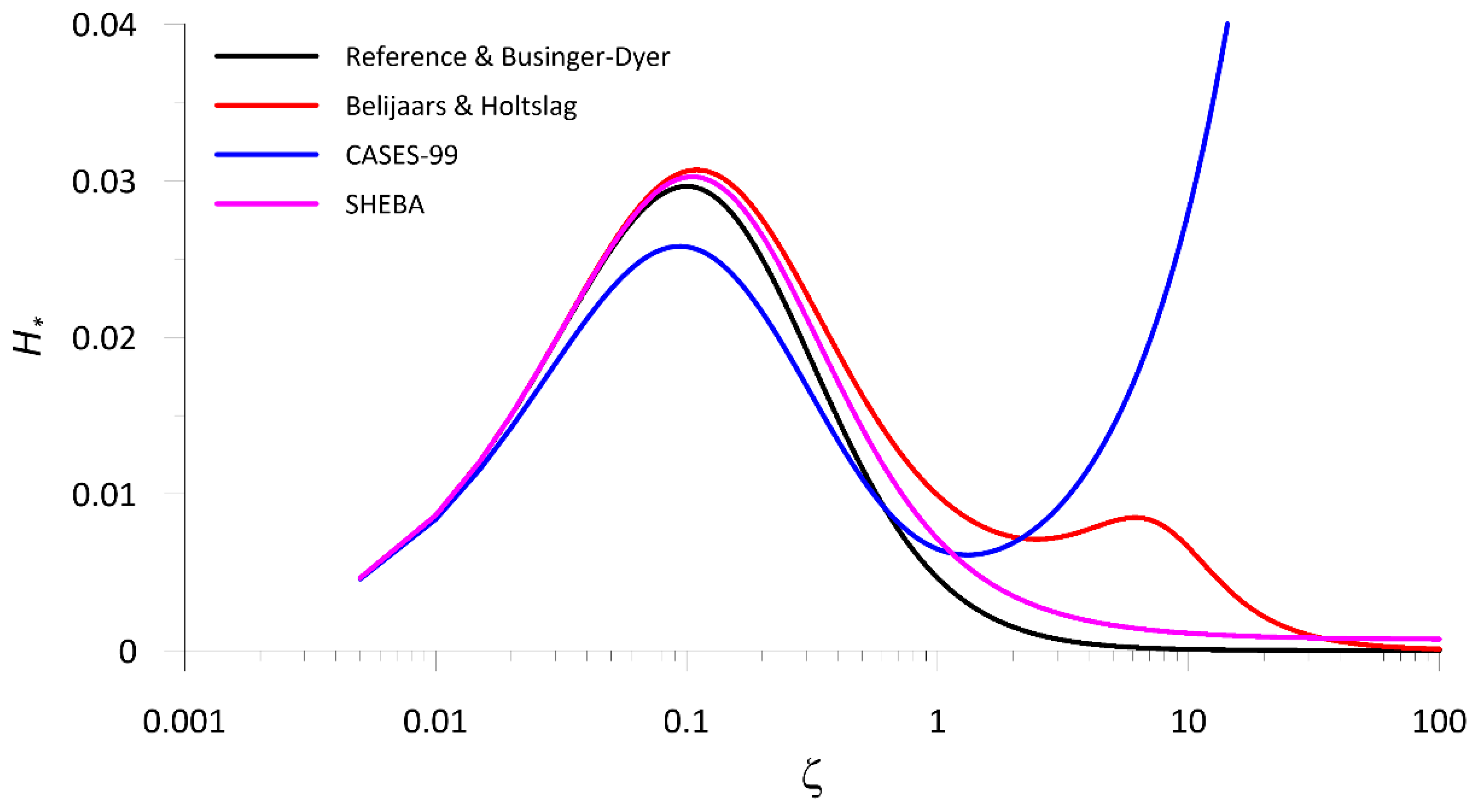
The behaviour of the absolute value of $H_{*}$ as a function of $\zeta$ for the four ${\mathsf{\Phi }}_m$ proposed in the literature is shown in Figure 1. Using Equation (7a) as a reference, the following conclusions can be made:

• SHEBA ${\mathsf{\Phi }}_m$ led to a trend similar to that expected, with a single maximum at $\zeta \cong 0.1$ and $H_{*}\to 0$ when $\zeta \to 0$ and $\zeta \to \infty$. We were not able to reproduce the local minimum at the large stability values ($\zeta \cong 80$) reported in [14].
• $H_{*}$ retrieved adopting the Beljaars–Holtslag ${\mathsf{\Phi }}_m$ presented a first maximum at $\zeta \cong 0.1$, but beyond that it did not decrease monotonically as expected, reaching a second maximum at $\zeta \cong 6.1$. The presence of such a secondary maximum might be attributed to the limited $\zeta$ values that can be observed at midlatitudes, i.e., where the Beljaars–Holtslag dataset was acquired.
• CASES-99 ${\mathsf{\Phi }}_m$ performance was disappointing, leading to a function that increased as stability increased.

As a result, while all equations were capable of reproducing the expected $H_{*}$ evolution when $0<\zeta \le 1$, both the Beljaars–Holtslag and the CASES-99 formulations did not hold under very stable conditions. When reference, Businger–Dyer, or SHEBA formulations were used, the correspondence between $\zeta$ and $H_{*}$ was not biunivocal and led to a sub- and a supercritical value of $\zeta$ for $H_{*}<H_{*,max}$.

The same analysis can be extended to the temperature scale $T_{*}$, whose expression as a function of ${\mathsf{\Phi }}_m\left(\zeta \right)$ was obtained from Equations (1) and (2a):

$$T_{*}=\frac{kz{\theta }_r}{g}\zeta {\left(\frac{dU/dz}{{\mathsf{\Phi }}_m\left(\zeta \right)}\right)}^2.$$

(15)

As before, it was convenient to introduce the dimensionless scale parameter $T_{**}$, that depends only on $\zeta$ and allows for direct comparisons between different ${\mathsf{\Phi }}_m\left(\zeta \right)$ expressions:

$$T_{**}=\frac{g}{kz{\theta }_r}{\left(dU/dz\right)}^{-2}{T}_{*}=\frac{\zeta }{{\left({\mathsf{\Phi }}_m\left(\zeta \right)\right)}^2}.$$

(16)

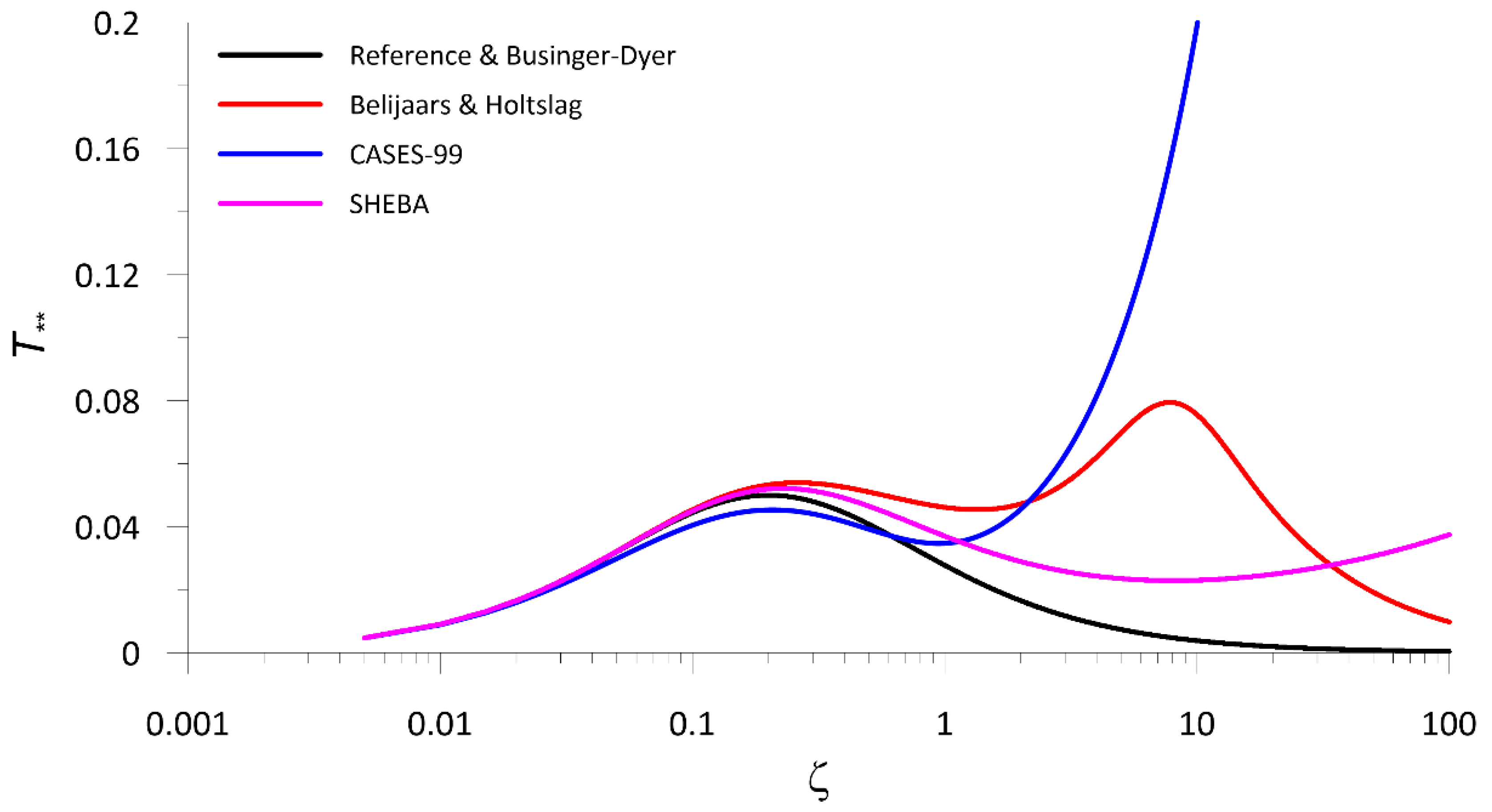
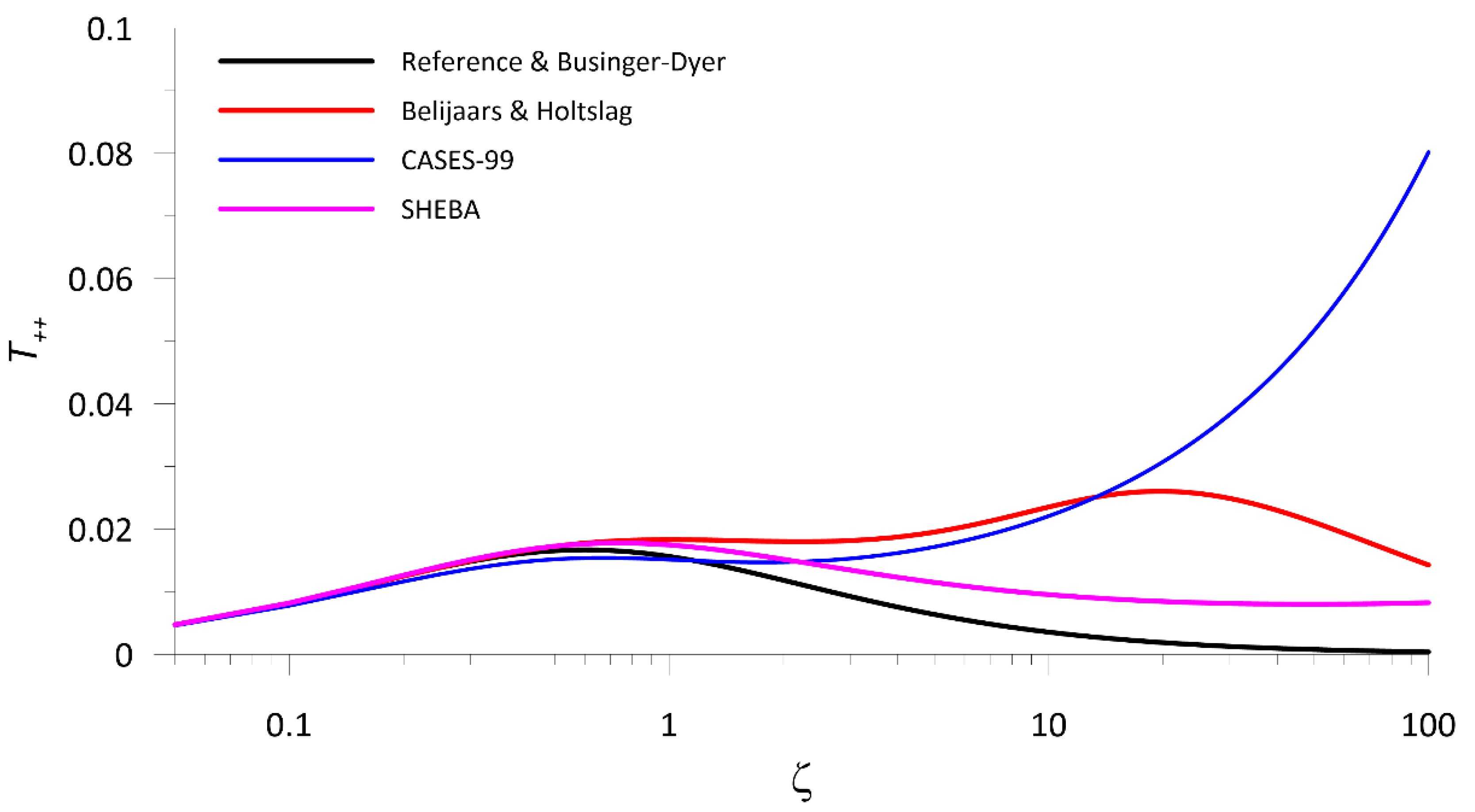
Since $T_{*}=-H_0/u_{*}$ and $u_{*}$ is greater than zero by definition (as long as $U>0$), all considerations of the evolution of $H_{*}$ as a function of $\zeta$ must hold here as well. Thus, $T_{**}$ is expected to tend to 0 when $\zeta \to 0$ and $\zeta \to \infty$ and to have a maximum somewhere between. When Equations (7a) or (8a) were used, the maximum value was at ${\zeta }_T=2{\zeta }_H\cong 0.2$, where $T_{**,max}=1/2{\beta }_m$. The behaviour of $T_{**}$ as a function of the stability parameter ζ for the four ${\mathsf{\Phi }}_m$ listed in Section 3 is represented in Figure 2, which shows how all functions except the reference and the Businger–Dyer ${\mathsf{\Phi }}_m$ led to unreliable representations of $T_{**}$ under very stable conditions. In particular, while all formulations presented a maximum at $\zeta \cong 0.2$, the Beljaars–Holtslag ${\mathsf{\Phi }}_m$ gave another pronounced maximum at $\zeta \cong 7.8$, and both CASES-99 and SHEBA ${\mathsf{\Phi }}_m$ did not approach to zero when $\zeta$ increased, presenting local minima at values of $\zeta$ that are of physical interest.

By inverting Equation (2b) is it possible to express $H$ as a function of ${\mathsf{\Phi }}_h\left(\zeta \right)$ instead of ${\mathsf{\Phi }}_m\left(\zeta \right)$, i.e., as a parametric equation where $H$ depends only on $\zeta$ when z and $d\theta /dz$ are fixed:

$$H={\left(\frac{g}{{\theta }_r}\right)}^{1/2}{\left(kz\right)}^2{\left(\frac{d\theta }{dz}\right)}^{3/2}{\zeta }^{-1/2}{\mathsf{\Phi }}_h^{-3/2}\left(\zeta \right).$$

(17)

Again, the dependence on $\zeta$ can be better studied by introducing the following dimensionless scale parameter:

$$H_{**}=H{\left(\frac{g}{{\theta }_r}\right)}^{-1/2}{\left(kz\right)}^{-2}{\left(\frac{d\theta }{dz}\right)}^{-3/2}={\zeta }^{-1/2}{\mathsf{\Phi }}_h^{-3/2}\left(\zeta \right).$$

(18)

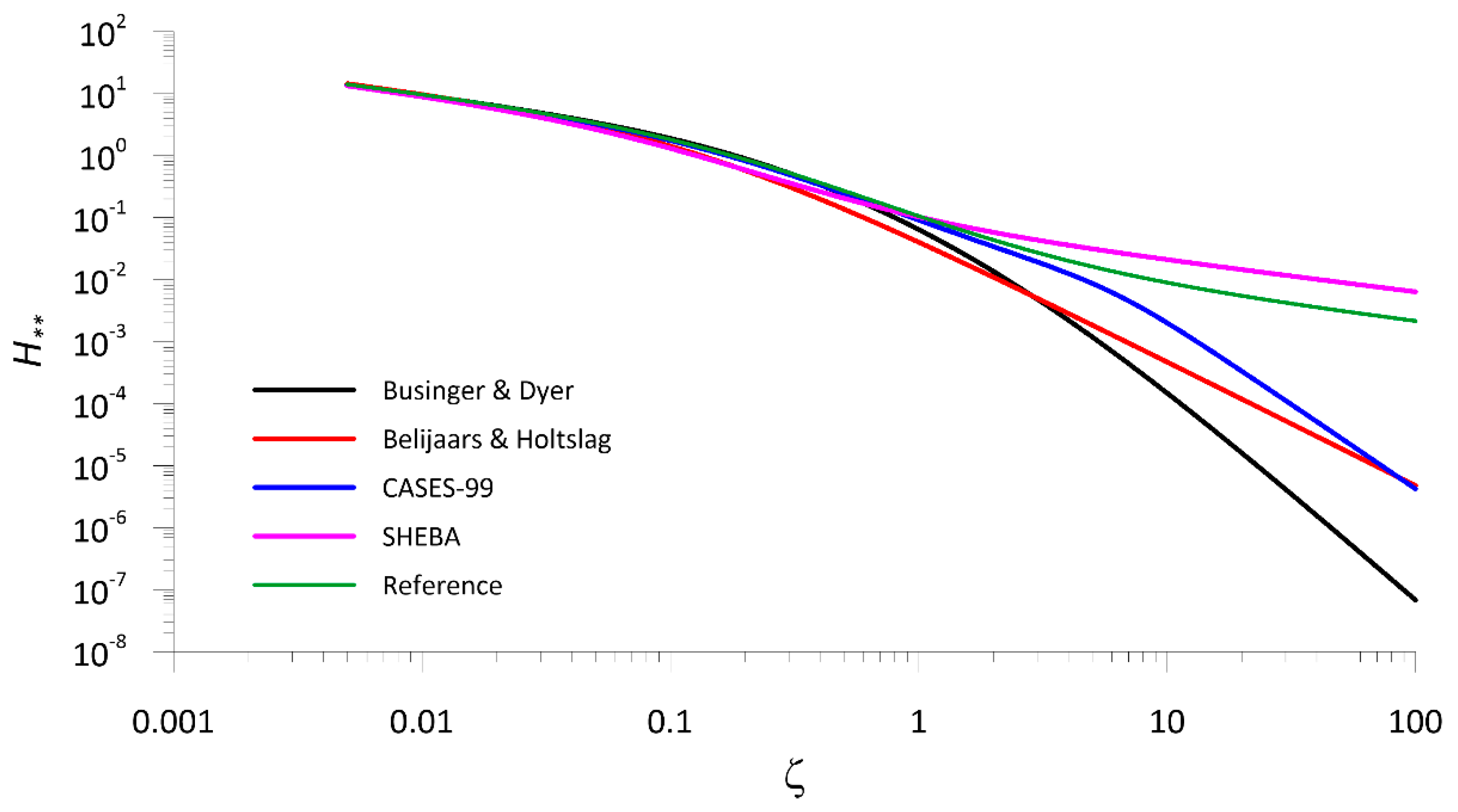
Unlike the previous cases, Equation (18) is not defined when $\zeta \to 0$, but it is straightforward to demonstrate that $H_{**}$ is represented by a monotonically decreasing function regardless of the analytical form of ${\mathsf{\Phi }}_h\left(\zeta \right)$. All the curves shown in Figure 3 tended to zero when $\zeta \to \infty$, even with different velocities depending on the ${\mathsf{\Phi }}_h$ chosen, with Businger–Dyer ${\mathsf{\Phi }}_h$ being the fastest and SHEBA the slowest. Moreover, SHEBA ${\mathsf{\Phi }}_h$ led to a trend very close to that of the reference function (7b), suggesting a very low influence of sub-meso motions. That is to say, the ${\mathsf{\Phi }}_h$ performance was even worse than that of ${\mathsf{\Phi }}_m$, leading to a monotonic trend that completely contradicted the expected behaviour.

4.2. Universal Functions for Wind and Temperature Profile

When measuring either the average wind speed or the mean potential temperature at a fixed height, the behaviour of both $H$ and $T_{*}$ can be expressed as a function of the universal similarity functions for wind and temperature gradient ${\mathsf{\Psi }}_m\left(\zeta \right)$ and ${\mathsf{\Psi }}_h\left(\zeta \right)$. In this case, the thermal and mechanical surface characteristics (represented by the three parameters $z_0$, $z_{0h}$, and ${\theta }_0$ in Equation (3) each play a role, and both $H_0$ and $T_{*}$ are now expected to depend on them.

Using Equation (3a) with $\zeta =z/L$ and Equation (1) gives

$$H=-H_0=\frac{{\theta }_r}{kzg}\zeta {\left[\frac{kU}{\ln \left(z/z_0\right)-{\mathsf{\Psi }}_m\left(\zeta \right)}\right]}^3,$$

(19)

that as its counterpart (12) is expected to tend to zero when $\zeta \to 0$ and $\zeta \to \infty$, i.e., to be described by a nonmonotonic function with one maximum. When the simple Businger–Dyer ${\mathsf{\Psi }}_m\left(\zeta \right)$ was used, it was easy to show [4] that Equation (18) has a maximum at ${\zeta }_H=\ln \left(z/z_0\right)/2{\beta }_m$, where $H_0$ is:

$$H_{max}=\frac{4k^2}{27}\frac{{\theta }_r}{zg{\beta }_m}\frac{U^3}{{\left[\ln \left(z/z_0\right)\right]}^2}.$$

(20)

Unlike the previous case, such a maximum is not universal, in the sense that it explicitly depends on the surface characteristics represented by $z_0$ and has to be considered as local.

As seen in the previous subsection, to compare the four ${\mathsf{\Psi }}_m$ proposed in the literature it is convenient to introduce the dimensionless variable

$$H_{+}=\frac{zg}{k^2}\frac{1}{{\theta }_r{U}^3}{H}^{\prime }=\frac{\zeta }{{\left[\ln \left(z/z_0\right)-{\mathsf{\Psi }}_m\left(\zeta \right)\right]}^3},$$

(21)

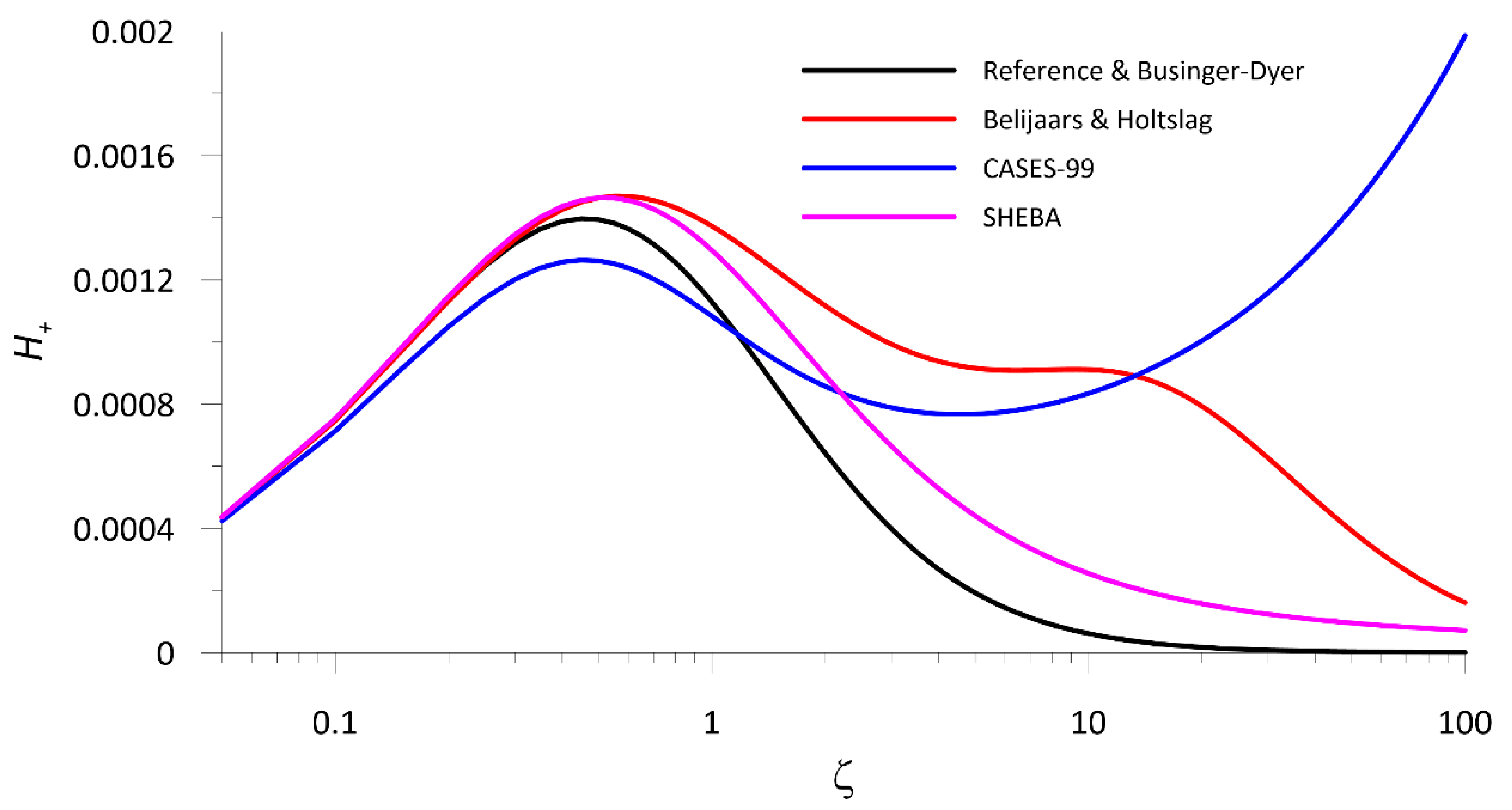
that is represented in Figure 4 as a function of $\zeta$ and for the five ${\mathsf{\Psi }}_m$ listed in Section 3, with $z_0$ = 0.1 m. The value of $z_0$ changed both the position of the maximum and its absolute value, but did not affect the general forms reported in Figure 4, which shows similar trends to those seen in the previous subsection. In particular, Businger–Dyer and reference ${\mathsf{\Psi }}_m$ (that coincided with each other), as well as SHEBA ${\mathsf{\Psi }}_m$, led to a $H_{*}$ trend compatible with that expected, but Beljaars–Holtslag ${\mathsf{\Psi }}_m$ produced a small secondary maximum around $\zeta \cong 10$ and CASES-99 formulation does not go to zero when $\zeta$ increased. All ${\mathsf{\Psi }}_m$ were capable of reproducing the first maximum, but in this case, it slightly depended on ${\mathsf{\Psi }}_m$ and was 0.46, 0.55, 0.45, and 0.5 for reference and Businger–Dyer, Beljaars–Holtslag, CASES-99, and SHEBA, respectively.

Regarding $T_{*}$, Equations (1) and (3a) gives

$$T_{*}=\frac{{\theta }_r}{kzg}\zeta {\left[\frac{kU}{\ln \left(z/z_0\right)-{\mathsf{\Psi }}_m\left(\zeta \right)}\right]}^2$$

(22)

and the dimensionless scale variable

$$T_{++}=\frac{zg}{{\theta }_r{U}^2}{T}_{*}=\frac{\zeta }{{\left[\ln \left(z/z_0\right)-{\mathsf{\Psi }}_m\left(\zeta \right)\right]}^2},$$

(23)

both of them depending on $z_0$. Once again, when the reference and the Businger–Dyer ${\mathsf{\Psi }}_m\left(\zeta \right)$ were selected it is easy to see that Equation (21) had its maximum value at ${\zeta }_T=\ln \left(z/z_0\right)/{\beta }_m=2{\zeta }_H$, where $T_{*}$ s

$$T_{*,max}=\frac{\theta {\mathsf{\Theta }}_r}{zg}\frac{k}{4{\beta }_m}\frac{U^2}{\ln \left(z/z_0\right)}$$

(24)

and depended on both $U$ and $z$, as well as on $z_0$. In addition, it is interesting to note that when $T_{*}$ was maximum $H$ was $\left({\zeta }_T\right)=27/32$ $H_{0,max}$, i.e., the two maxima were not coincident.

Figure 5 shows the comparison between different $T_{++}$ numerically calculated as a function of $\zeta$ for the four available ${\mathsf{\Psi }}_m$ with $z_0$ = 0.1 m. Moreover, in this case, $z_0$ did not affect the general behaviour of $T_{**}$ and the trends illustrated in Figure 5 can be considered as representative. The reference and Businger–Dyer ${\mathsf{\Psi }}_m$ led to the expected $T_{++}$ trend, reaching a maximum around $\zeta =1$ and decreasing as stability increased. SHEBA ${\mathsf{\Psi }}_m$ had similar behaviour, but with a slower decreasing trend reaching a slight minimum at high $\zeta$ values. In contrast, both the Beljaars–Holtslag and the CASES-99 formulations led to unreliable results, and did not appear to be capable of reproducing the expected behaviour. In particular, CASES-99 ${\mathsf{\Psi }}_m$ did not lead to a decreasing trend at all.

Following the same analysis performed in the previous subsection, it is possible to express $H$ as a function of ${\mathsf{\Psi }}_h$ also in this case, i.e., when dealing with profile universal functions. Obtaining $T_{*}$ from Equation (3b) and substituting it into $\zeta =z/L=kzg/{\theta }_r\cdot T_{*}/u_{*}^2$ to obtain $u_{*}$, $H=-T_{*}{u}_{*}$ can be expressed as

$$H=\sqrt{\frac{kzg}{{\theta }_r}}{\zeta }^{-1/2}{\left(\frac{k\left(\theta -{\theta }_0\right)}{\ln \left(z/z_{0h}\right)-{\mathsf{\Psi }}_h\left(\zeta \right)}\right)}^{3/2} ,$$

(25)

that leads to the dimensionless parameter

$$H_{++}=\sqrt{\frac{{\theta }_r}{kzg}}{\left(\frac{1}{k\left(\theta -{\theta }_0\right)}\right)}^{3/2}H=\frac{{\zeta }^{-1/2}}{{\left(\ln \left(z/z_{0h}\right)-{\mathsf{\Psi }}_h\left(\zeta \right)\right)}^{3/2}} .$$

(26)

Similarly to $H_{**}$, $H_{++}$ is not defined when $\theta -{\theta }_0=0$ Whatever ${\mathsf{\Psi }}_h\left(\zeta \right)$ and $z_{0h}$ values were used, $H_{++}$ trends were analogous to those presented in Figure 3, i.e., monotonically decreasing functions without extrema. Again, none of the published ${\mathsf{\Psi }}_h\left(\zeta \right)$ were capable of reproducing the expected behavior.

5. Discussion

Theoretical and experimental results suggest that both $H$ and $T_{*}$ tend to zero when $\zeta$ goes to zero or infinity, reaching a maximum in correspondence of the critical values ${\zeta }_H$ and ${\zeta }_T$, that discriminate between continuous and intermittent turbulence. In particular, when stability reaches supercritical values, turbulence becomes weak and can be significantly inflated by the presence of nonturbulent motions.

Assuming that MOST is a suitable theory to describe SBL turbulence under both weak and strong stability conditions, the behaviour of $H$ and $T_{*}$ as a function of different universal similarity functions was systematically investigated. The analysis included four experimentally determined formulations, as well as a reference formulation estimated from theoretical considerations and LES (i.e., expected to be valid under neutral condition and for homogeneous and stationary turbulence). Both the reference and the four experimentally determined formulations for ${\mathsf{\Phi }}_m$, ${\mathsf{\Phi }}_h$ ${\mathsf{\Psi }}_m$, and ${\mathsf{\Psi }}_h$ used here were expected to lead to similar outcomes, but our analysis showed otherwise. All ${\mathsf{\Phi }}_m$ and ${\mathsf{\Psi }}_m$ were able to describe the expected $H$ and $T_{*}$ trends for subcritical values of $\zeta$ ($\zeta <{\zeta }_{H,T}$), including their maxima. Such a result is not surprising, as when neutrality is approached (i.e., when $\zeta \to 0$) Beljaars–Holtslag, CASES-99, and SHEBA formulations reduce to the equations proposed by Businger and Dyer (although with different coefficients). Nevertheless, for supercritical values ($\zeta >{\zeta }_{H,T}$), three out of four formulations (namely Beljaars–Holtslag, CASES-99, and SHEBA) led to unreliable results, with varying degrees of failure. In particular, the SHEBA formulation showed an appreciable deviation only from the expected $T_{*}$ trend at high $\zeta$ values, while the Belijaars–Holtslag formulation always presented another pronounced maximum, and CASES-99 did not tend to zero as $\zeta$ increased. When considering ${\mathsf{\Phi }}_h$ and ${\mathsf{\Psi }}_h$ functions, the results were even more disappointing, as none of the formulations (including the reference) were able to reproduce the expected behaviour. Such results are difficult to explain without reanalysing the original datasets from which the universal similarity functions were obtained, but some useful remarks can still be made.

Firstly, all experimental campaigns did not explicitly take into account nonturbulent motions, which can sensibly affect turbulence measurements especially under very stable conditions, when the stability parameter $\zeta$ exceeds its critical value. Excluding nonturbulent motion would require a completely different data analysis based on the spectral gap that separates the small-scale turbulent region from mesoscale and sub-mesoscale motions [20,21,52]. Starting from this evidence, a multiresolution decomposition technique was successfully implemented in [22] to determine a turbulence cutoff time scale closely related to the spectral gap. This result was further extended in [34], where the authors introduced a variable averaging time $\tau$, based on the bulk Richardson number (their Equations (12) and (13)), that varied between 20 min (strongly unstable conditions) and 30 s (strongly stable conditions). As demonstrated in [19], such an approach is effective in removing most of the nonturbulent perturbations, with the exception of Kelvin–Helmholtz shear instability.

Secondly, none of the analysed formulations considered the possible presence of self-correlation, which may affect the regression analysis yielding unreliable results, as well demonstrated in [5,53]. For instance, ${\mathsf{\Phi }}_m\left(\zeta \right)$ is usually retrieved from Equation (2) by performing a curve fit of the measured ${\mathsf{\Phi }}_m\left(\zeta \right)=\frac{kz}{u_{*}}\frac{dU}{dz}$, where the friction velocity $u_{*}$ is present in both the dependent and the independent variable.

This problem is also related to how flux–profile relationships are determined. All the formulations considered here were obtained independently of each other, thus neglecting any possible physical constraints or relation between them, but MOST requires for universal functions to be congruent with all the similarity relationships in which they are included. To be clearer, let us focus only on ${\mathsf{\Phi }}_m$ and ${\mathsf{\Phi }}_h$, although a similar reasoning applies to ${\mathsf{\Psi }}_m$, and ${\mathsf{\Psi }}_h$ as well. In a typical experimental campaign, they are retrieved separately by measuring $dU/dz$, $d\theta /dz$, $u_{*}$, and $T_{*}$, so that any possible physical relationships between them is neglected. To overcome such an issue, let us recall that there are three possible parameters to characterize stability strength: the stability parameter $\zeta$, which at a fixed height depends only on the turbulent SBL parameters $u_{*}$ and $T_{*}$; the gradient Richardson numbers, defined only by mean parameters such as the lapse rate and the gradients of the mean horizontal wind speed components; and the flux Richardson number, which depends on a combination of both turbulent and mean parameters. As anticipated in Section 2, the gradient Richardson number can be written as a function of both ${\mathsf{\Phi }}_m$ and ${\mathsf{\Phi }}_h:$

$$Ri=\zeta \frac{{\mathsf{\Phi }}_h\left(\zeta \right)}{{\left({\mathsf{\Phi }}_m\left(\zeta \right)\right)}^2}={\mathfrak{J}}_{R_i}\left(\zeta \right),$$

(27)

that is a similar relationship between $Ri$ and $\zeta$ not affected by self-correlation. Moreover, ${\mathfrak{J}}_{Ri}\left(\zeta \right)$ represents a constraint that both ${\mathsf{\Phi }}_h\left(\zeta \right)$ and ${\mathsf{\Phi }}_m\left(\zeta \right)$ need to satisfy, as well as the absence of a critical value for $Ri$. Equation (27) alone would not enable determination of the two universal functions separately, just the functional form of their ratio. Nevertheless, Equation (27) could be used in conjunction with its equivalent for $Rf$,

$$Rf=\frac{\zeta }{{\mathsf{\Phi }}_m\left(\zeta \right)}={\mathfrak{J}}_{Rf}\left(\zeta \right),$$

(28)

that does not involve ${\mathsf{\Phi }}_h\left(\zeta \right)$ but presents self-correlations that would need to be addressed and is expected to reach a critical value when $\zeta \to \infty$.

Such an approach, along with a careful data analysis to exclude the presence of nonturbulent motions, could contribute to determining universal similarity functions that are consistent with both the flux–profile relationships and the variety of physical processes observed in the SBL. The effectiveness of this approach will be tested in future work, where data acquired at Concordia station (Dome C, Antarctica) under stable and strongly stable conditions will be analysed following the recommendations described above.

References

- Mahrt, L. Nocturnal boundary-layer regimes. Bound.-Layer Meteorol. 1998, 88, 255–278. [Google Scholar] [CrossRef]
- Mahrt, L. Stratified atmospheric boundary layers and breakdown of models. Theor. Comput. Fluid Dyn. 1998, 11, 263–279. [Google Scholar] [CrossRef]
- De Bruin, H.A.R. Analytic solutions of the equations governing the temperature fluctuation method. Bound.-Layer Meteorol. 1994, 68, 427–432. [Google Scholar] [CrossRef]
- Malhi, Y.S. The significance of the dual solutions for heat fluxes measured by the temperature fluctuation method in stable conditions. Bound.-Layer Meteorol. 1995, 74, 389–396. [Google Scholar] [CrossRef]
- Grachev, A.A.; Fairall, C.W.; Persson, P.O.G.; Andreas, E.L.; Guest, P.S. Stable Boundary-Layer Scaling Regimes: The Sheba Data. Bound.-Layer Meteorol. 2005, 116, 201–235. [Google Scholar] [CrossRef]
- Basu, S.; Holtslag, B.; Van De Wiel, B.J.H.; Moene, A.; Steeneveld, G.-J. An inconvenient “truth” about using sensible heat flux as a surface boundary condition in models under stably stratified regimes. Acta Geophys. 2007, 56, 88–99. [Google Scholar] [CrossRef] [Green Version]
- Sorbjan, Z. Local structure of turbulence in stably stratified boundary layers. J. Atmos. Sci. 2006, 63, 1526–1537. [Google Scholar] [CrossRef] [Green Version]
- Van de Wiel, B.J.H.; Vignon, E.; Baas, P.; van Hooijdonk, I.G.S.; van der Linden, S.J.A.; van Hooft, J.A.; Bosveld, F.C.; de Roode, S.R.; Moene, A.F.; Genthon, C. Regime transitions in near-surface temperature inversions: A conceptual model. J. Atmos. Sci. 2017, 74, 1057–1073. [Google Scholar] [CrossRef] [Green Version]
- Van De Wiel, B.J.H.; Moene, A.F.; Jonker, H.J.J. The Cessation of continuous turbulence as precursor of the very stable nocturnal boundary layer. J. Atmos. Sci. 2012, 69, 3097–3115. [Google Scholar] [CrossRef] [Green Version]
- Van De Wiel, B.J.H.; Moene, A.F.; Jonker, H.J.J.; Baas, P.; Basu, S.; Donda, J.M.M.; Sun, J.; Holtslag, A.A.M. The minimum wind speed for sustainable turbulence in the nocturnal boundary layer. J. Atmos. Sci. 2012, 69, 3116–3127. [Google Scholar] [CrossRef] [Green Version]
- van de Wiel, B.J.H.; Basu, S.; Moene, A.F.; Jonker, H.J.J.; Steeneveld, G.J.; Holtslag, A.A.M. Comments on “An extremum solution of the Monin-Obukhov similarity equations”. J. Atmos. Sci. 2011, 68, 1405–1408. [Google Scholar] [CrossRef]
- van de Wiel, B.J.H.; Moene, A.F.; Steeneveld, G.J.; Hartogensis, O.K.; Holtslag, A.A.M. Predicting the collapse of turbulence in stably stratified boundary layers. Flow Turbul. Combust. 2007, 79, 251–274. [Google Scholar] [CrossRef] [Green Version]
- Wang, J.; Bras, R.L. An extremum solution of the Monin–Obukhov similarity equations. J. Atmos. Sci. 2010, 67, 485–499. [Google Scholar] [CrossRef]
- Srivastava, P.; Sharan, M. Analysis of dual nature of heat flux predicted by Monin-Obukhov similarity theory: An impact of empirical forms of stability correction functions. J. Geophys. Res. Atmos. 2019, 124, 3627–3646. [Google Scholar] [CrossRef]
- Mahrt, L. The influence of nonstationarity on the turbulent flux–gradient relationship for stable stratification. Bound.-Layer Meteorol. 2007, 125, 245–264. [Google Scholar] [CrossRef]
- Basu, S.; Porté-Agel, F.; Foufoula-Georgiou, E.; Vinuesa, J.-F.; Pahlow, M. Revisiting the local scaling hypothesis in stably stratified atmospheric boundary-layer turbulence: An integration of field and laboratory measurements with large-eddy simulations. Bound.-Layer Meteorol. 2005, 119, 473–500. [Google Scholar] [CrossRef] [Green Version]
- Luhar, A.K.; Rayner, K.N. Methods to estimate surface fluxes of momentum and heat from routine weather observations for dispersion applications under stable stratification. Bound.-Layer Meteorol. 2009, 132, 437–454. [Google Scholar] [CrossRef]
- Luhar, A.K.; Hurley, P.J.; Rayner, K.N. Modelling near-surface low winds over land under stable conditions: Sensitivity tests, flux-gradient relationships, and stability parameters. Bound.-Layer Meteorol. 2008, 130, 249–274. [Google Scholar] [CrossRef]
- Cheng, Y.; Parlange, M.B.; Brutsaert, W. Pathology of Monin-Obukhov similarity in the stable boundary layer. J. Geophys. Res. Space Phys. 2005, 110, D06101. [Google Scholar] [CrossRef] [Green Version]
- Vickers, D.; Mahrt, L. A solution for flux contamination by mesoscale motions with very weak turbulence. Bound.-Layer Meteorol. 2005, 118, 431–447. [Google Scholar] [CrossRef]
- Mahrt, L.; Moore, E.; Vickers, D.; Jensen, N.O. Dependence of turbulent and mesoscale velocity variances on scale and stability. J. Appl. Meteorol. 2001, 40, 628–641. [Google Scholar] [CrossRef]
- Howell, J.F.; Sun, J. Surface-layer fluxes in stable conditions. Bound.-Layer Meteorol. 1999, 90, 495–520. [Google Scholar] [CrossRef]
- Galperin, B.; Sukoriansky, S.; Anderson, P.S. On the critical Richardson number in stably stratified turbulence. Atmos. Sci. Lett. 2007, 8, 65–69. [Google Scholar] [CrossRef]
- Zilitinkevich, S.S.; Elperin, T.; Kleeorin, N.; L’Vov, V.; Rogachevskii, I. Energy- and flux-budget turbulence closure model for stably stratified flows. Part II: The role of internal gravity waves. Bound.-Layer Meteorol. 2009, 133, 139–164. [Google Scholar] [CrossRef] [Green Version]
- Tennekes, H. Similarity relations, scaling laws and spectral dynamics. In Atmospheric Turbulence and Air Pollution Modelling; Nieuwstadt, F.T.M., van Dop, H., Eds.; Springer: Dordrecht, The Netherlands, 1984; pp. 37–68. [Google Scholar] [CrossRef]
- Zilitinkevich, S.S.; Esau, I.; Kleeorin, N.; Rogachevskii, I.; Kouznetsov, R. On the velocity gradient in stably stratified sheared flows. part 1: Asymptotic analysis and applications. Bound.-Layer Meteorol. 2010, 135, 505–511. [Google Scholar] [CrossRef] [Green Version]
- Yamada, T. The critical Richardson number and the ratio of the Eddy transport coefficients obtained from a turbulence closure model. J. Atmos. Sci. 1975, 32, 926–933. [Google Scholar] [CrossRef]
- Zilitinkevich, S.S.; Elperin, T.; Kleeorin, N.; Rogachevskii, I.; Esau, I.; Mauritsen, T.; Milesf, M.W. Turbulence energetics in stably stratified geophysical flows: Strong and weak mixing regimes. Q. J. R. Meteorol. Soc. 2008, 134, 793–799. [Google Scholar] [CrossRef] [Green Version]
- Zilitinkevich, S.S.; Elperin, T.; Kleeorin, N.; Rogachevskii, I. Energy- and flux-budget (EFB) turbulence closure model for stably stratified flows. Part I: Steady-state, homogeneous regimes. Bound.-Layer Meteorol. 2007, 125, 167–191. [Google Scholar] [CrossRef] [Green Version]
- Mauritsen, T.; Svensson, G. Observations of stably stratified shear-driven atmospheric turbulence at low and high richardson numbers. J. Atmos. Sci. 2007, 64, 645–655. [Google Scholar] [CrossRef]
- Mauritsen, T.; Svensson, G.; Zilitinkevich, S.S.; Esau, I.; Enger, L.; Grisogono, B. A total turbulent energy closure model for neutrally and stably stratified atmospheric boundary layers. J. Atmos. Sci. 2007, 64, 4113–4126. [Google Scholar] [CrossRef]
- Venayagamoorthy, S.K.; Stretch, D. On the turbulent Prandtl number in homogeneous stably stratified turbulence. J. Fluid Mech. 2010, 644, 359–369. [Google Scholar] [CrossRef] [Green Version]
- Kouznetsov, R.D.; Zilitinkevich, S. On the velocity gradient in stably stratified sheared flows. Part 2: Observations and models. Bound.-Layer Meteorol. 2010, 135, 513–517. [Google Scholar] [CrossRef] [Green Version]
- Vickers, D.; Mahrt, L. The cospectral gap and turbulent flux calculations. J. Atmos. Ocean. Technol. 2003, 20, 660–672. [Google Scholar] [CrossRef]
- Nappo, C.J. An Introduction to Atmospheric Gravity Waves, 2nd ed.; Academic Press: Cambridge, MA, USA, 2012. [Google Scholar]
- Businger, J.A.; Wyngaard, J.C.; Izumi, Y.; Bradley, E.F. Flux-profile relationships in the atmospheric surface layer. J. Atmos. Sci. 1971, 28, 181–189. [Google Scholar] [CrossRef]
- Dyer, A.J. A review of flux-profile relationships. Bound.-Layer Meteorol. 1974, 7, 363–372. [Google Scholar] [CrossRef]
- Hicks, B.B. Wind profile relationships from the ‘wangara’ experiment. Q. J. R. Meteorol. Soc. 1976, 102, 535–551. [Google Scholar] [CrossRef]
- Högström, U.; Bergström, H.; Smedman, A.-S.; Halldin, S.; Lindroth, A. Turbulent exchange above a pine forest, I: Fluxes and gradients. Bound.-Layer Meteorol. 1989, 49, 197–217. [Google Scholar] [CrossRef]
- Högström, U. Non-dimensional wind and temperature profiles in the atmospheric surface layer: A re-evaluation. Bound.-Layer Meteorol. 1988, 42, 55–78. [Google Scholar] [CrossRef]
- Högström, U. Review of some basic characteristics of the atmospheric surface layer. Bound.-Layer Meteorol. 1996, 78, 215–246. [Google Scholar] [CrossRef]
- Webb, E.K. Profile relationships: The log-linear range, and extension to strong stability. Q. J. R. Meteorol. Soc. 1970, 96, 67–90. [Google Scholar] [CrossRef]
- Carson, D.J.; Richards, P.J.R. Modelling surface turbulent fluxes in stable conditions. Bound.-Layer Meteorol. 1978, 14, 67–81. [Google Scholar] [CrossRef]
- Van Ulden, A.P.; Holtslag, A.A.M. Estimation of atmospheric boundary layer parameters for diffusion applications. J. Clim. Appl. Meteorol. 1985, 24, 1196–1207. [Google Scholar] [CrossRef] [Green Version]
- Beljaars, A.C.M.; Holtslag, A.A.M. Flux parameterization over land surfaces for atmospheric models. J. Appl. Meteorol. 1991, 30, 327–341. [Google Scholar] [CrossRef]
- Stull, R.B. An Introduction to Boundary Layer Meteorology; Springer: Dordrecht, The Netherlands, 1988. [Google Scholar]
- Poulos, G.S.; Blumen, W.; Fritts, D.C.; Lundquist, J.K.; Sun, J.; Burns, S.P.; Nappo, C.; Banta, R.; Newsom, R.; Cuxart, J.; et al. CASES-99: A comprehensive investigation of the stable nocturnal boundary layer. Bull. Am. Meteorol. Soc. 2002, 83, 555–581. [Google Scholar] [CrossRef]
- Chenge, Y.; Brutsaert, W. Flux-profile relationships for wind speed and temperature in the stable atmospheric boundary layer. Bound.-Layer Meteorol. 2005, 114, 519–538. [Google Scholar] [CrossRef]
- Uttal, T.; Curry, J.A.; McPhee, M.G.; Perovich, D.K.; Moritz, R.E.; Maslanik, J.A.; Guest, P.S.; Stern, H.L.; Moore, J.A.; Turenne, R.; et al. Surface heat budget of the Arctic Ocean. Bull. Am. Meteorol. Soc. 2002, 83, 255–275. [Google Scholar] [CrossRef] [Green Version]
- Grachev, A.A.; Andreas, E.L.; Fairall, C.; Guest, P.S.; Persson, P.O.G. SHEBA flux–profile relationships in the stable atmospheric boundary layer. Bound.-Layer Meteorol. 2007, 124, 315–333. [Google Scholar] [CrossRef]
- Gryanik, V.M.; Lüpkes, C.; Grachev, A.; Sidorenko, D. New modified and extended stability functions for the stable boundary layer based on SHEBA and parametrizations of bulk transfer coefficients for climate models. J. Atmos. Sci. 2020, 77, 2687–2716. [Google Scholar] [CrossRef]
- Smedman-Högström, A.-S.; Högström, U. Spectral gap in surface-layer measurements. J. Atmos. Sci. 1975, 32, 340–350. [Google Scholar] [CrossRef] [Green Version]
- Klipp, C.L.; Mahrt, L. Flux–gradient relationship, self-correlation and intermittency in the stable boundary layer. Q. J. R. Meteorol. Soc. 2004, 130, 2087–2103. [Google Scholar] [CrossRef]
Figure 1.
Evolution of as a function of the stability parameter for the four listed in Section 3.
Figure 2.
Figure 3.
Evolution of the absolute value of as a function of the stability parameter for the four listed in Section 3.
Figure 4.
Evolution of the absolute value of as a function of the stability parameter for the four listed in Section 3 ( = 0.5 m).
Figure 5.
Evolution of as a function of the stability parameter for the four listed in Section 3 ( = 0.5 m).
Publisher’s Note: MDPI stays neutral with regard to jurisdictional claims in published maps and institutional affiliations. |
© 2021 by the authors. Licensee MDPI, Basel, Switzerland. This article is an open access article distributed under the terms and conditions of the Creative Commons Attribution (CC BY) license (https://creativecommons.org/licenses/by/4.0/).
Share and Cite
MDPI and ACS Style
Casasanta, G.; Sozzi, R.; Petenko, I.; Argentini, S. Flux–Profile Relationships in the Stable Boundary Layer—A Critical Discussion. Atmosphere 2021, 12, 1197. https://0-doi-org.brum.beds.ac.uk/10.3390/atmos12091197
AMA Style
Casasanta G, Sozzi R, Petenko I, Argentini S. Flux–Profile Relationships in the Stable Boundary Layer—A Critical Discussion. Atmosphere. 2021; 12(9):1197. https://0-doi-org.brum.beds.ac.uk/10.3390/atmos12091197
Chicago/Turabian StyleCasasanta, Giampietro, Roberto Sozzi, Igor Petenko, and Stefania Argentini. 2021. "Flux–Profile Relationships in the Stable Boundary Layer—A Critical Discussion" Atmosphere 12, no. 9: 1197. https://0-doi-org.brum.beds.ac.uk/10.3390/atmos12091197
Note that from the first issue of 2016, this journal uses article numbers instead of page numbers. See further details here.