Article

Temporal Variability and Predictability of Intense Cyclones in the Western and Eastern Mediterranean

by
Veronika N. Maslova
*,
Elena N. Voskresenskaya
,
Andrey S. Lubkov
and
Alexander V. Yurovsky
Institute of Natural and Technical Systems, 299011 Sevastopol, Russia
*
Author to whom correspondence should be addressed.
Submission received: 15 July 2021 / Revised: 10 September 2021 / Accepted: 14 September 2021 / Published: 17 September 2021

Abstract

:
Our understanding of the time variability of intense cyclones in the Mediterranean region is still lacking despite its importance for the long-term forecast of climate anomalies. This study examines the month-to-month variability and predictability of cyclones, the intensity of which exceeded the 75th percentile (intense cyclones) and the 95th percentile (extreme cyclones), over the Western and Eastern Mediterranean. The locations of cyclones were obtained by applying the method of M. Yu. Bardin on the 6-hourly 1000 hPa geopotential height data from the NCEP/NCAR reanalysis for the period 1951–2017 (67 years). It was shown that annual frequencies of cyclones were higher in the Western Mediterranean due to the contribution of spring and autumn; monthly averages were higher in the Eastern Mediterranean in December/January–March for intense/extreme cyclones. In the context of global warming, no linear trends significant at the 90% confidence level were found in the variability of intense and extreme cyclones, except for a positive trend in autumn extreme cyclones over the Eastern Mediterranean. The time series of cyclones in both parts of the Mediterranean were characterized by a pronounced interannual variability with a noticeable decadal modulation. According to spectral analysis, these interannual periods were multiples of 2–3 years corresponding to the main global teleconnection patterns. Seasonally, the most energy was concentrated in winter spectra; spring and autumn spectra had lower comparable magnitudes. The correlation analysis between the frequency of cyclones and the indices of the main atmospheric patterns showed that the main synchronous patterns for intense and extreme Mediterranean cyclones in September–April were the Mediterranean Oscillation (with the opposite signs for the Western and Eastern Mediterranean), Scandinavia pattern (positive correlation), and East Atlantic Oscillation (negative correlation). Additional important synchronous teleconnection patterns for some months were the Arctic Oscillation and East Atlantic/West Russia pattern for the Western Mediterranean, and the Polar/Eurasia pattern and Tropical Northern Hemisphere pattern for the Eastern Mediterranean. The outcome of this paper was the use of an artificial neural network model with inputs of global teleconnection indices both in the atmosphere and ocean to describe the temporal variability of the frequency of intense cyclones in the Western and Eastern Mediterranean. The predictability of intense cyclones was shown with the possibility of forecasts with a lead time of 0, 2, 4, and 6 months for the Western Mediterranean in October, January, February, April, and May, and for the Eastern Mediterranean in January, February, March, April, and May. One of the applications of this model may be in forecasting the evolution of the monthly frequency of cyclones with a lead time of 2 to 6 months.

1. Introduction

The Mediterranean region is an important center of high cyclonic activity over the Northern Hemisphere, after the North Atlantic and North Pacific centers [1]. Due to geographical and orographic features, air masses over the Mediterranean Sea in winter have great contrasts of temperature and moisture content: cold air masses are located to the north of the mountain ranges over Europe, and tropical air spreads almost unhindered to the Mediterranean Sea. In winter, a latitudinal frontal zone with large baric and thermal gradients is established over the northern part of the Mediterranean Sea, which has the characteristics of a seasonal quasi-stationary front along which Mediterranean cyclones form [2].
The formation and evolution of Mediterranean cyclones is determined mainly by the interaction between the large-scale average flow in the atmosphere and local geomorphological features. Upper tropospheric forcing brings potential vorticity in the upper troposphere. At the same time, the mountain ridges around the basin and a complex land–sea distribution produce disturbances at the surface level. According to [3], cyclones over the Mediterranean region are essentially subsynoptic lows in winter (triggered by the North Atlantic synoptic systems being affected by local orography and/or low-level baroclinicity over the northern Mediterranean coast) and thermally induced lows in summer, despite the existence of other factors, such as the Atlas Mountains contributing to lee cyclogenesis in Northern Africa, or the extension of the Asian monsoon into the eastern part of the Mediterranean.
The most active cyclogenesis areas over the Mediterranean region, according to [3,4,5,6], are located mostly along the northern coast in winter (e.g., the Gulf of Genoa/Ligurian Sea, Aegean Sea, Black Sea, Balearic Sea, Gulf of Lyon, Adriatic Sea, Ionic Sea, Crete) and along the southern, western, and eastern coasts in summer (e.g., Iberian Peninsula, the southern slopes of the Atlas Mountains, Gulf of Gabes, Gulf of Sidra, Cyprus). Explosive cyclones tend to form in the Western Mediterranean, though their scale and depth is greater in the Eastern Mediterranean [7].
The study of the variability of intense cyclones is an important aspect of recent research on the patterns and mechanisms of regional environmental change. Knowledge about these patterns is necessary for the development of the theory of long-term forecasts of weather and climate anomalies. At the same time, intense cyclones in the Mediterranean region cause dangerous weather phenomena, such as extreme precipitation [8], wind storms [9], extreme waves [10], floods [11], landslides [12], thunderstorms [13], and even extreme dust events [14]. Quite often, they bring negative consequences to regions far from their place of origin, in particular, Central and Eastern Europe, the Middle East, and even Central Asia. Such extreme events can damage the environment and socioeconomic welfare [15], especially in the Mediterranean region with active slope and coastal processes [16].
Researchers usually study intense cyclones in the Mediterranean in terms of physical and thermodynamic processes, e.g., in [17], but not in terms of their temporal variability, which is better shown for the total frequency of cyclones, e.g., in [18]. A systematic climatology of Mediterranean cyclones has been studied, e.g., in [19,20], and included in the tasks of the following international projects: Mediterranean Cyclones Study Project (MCP) [21], MedCLIVAR [22,23], and MEDEX [24]. The Mediterranean Climate Variability and Predictability (MedCLIVAR) program serves as a scientific network to promote better communication among different scientific disciplines and to develop a multidisciplinary vision of the evolution of the Mediterranean climate [22]. The general objective of the international MEDiterranean EXperiment (MEDEX) was a better understanding and forecasting of cyclones that produce high-impact weather in the Mediterranean [24]. This is why our study is focused not on the climatological values and other characteristics of intense cyclones, but on their interannual fluctuations for the purposes of further forecasting monthly values.
The main temporal scales of regional climate fluctuations are associated with global processes in the ocean–atmosphere system. The centers of the most active ocean–atmosphere interaction are characterized by the strongest correlation with climate anomalies. In the atmosphere, they correspond to semi-permanent centers of high/low pressure (so-called atmospheric centers of action, for example in [25]). In the ocean, they are linked to the regions with the strongest sensible and latent heat fluxes, for example, the Gulf Stream region near Newfoundland (so-called energy-active zones of the World Ocean [26]). These global processes are referred to as teleconnection patterns [27,28] and are described by simple indices (calculated using spatial correlation analysis or principal component analysis) that can be used as predictors for regional climatic anomalies. Teleconnection patterns are associated with the modes of general atmospheric circulation by influencing its elements, such as the mean flow, baric anomalies, gradients and fronts, synoptic systems, heat and moisture transport, intensity and location of the jet stream, and storm track [29,30,31,32,33,34].
Oceanic patterns are characterized by several modes of low-frequency variability [28]. The main patterns are the Atlantic Multidecadal Oscillation [35,36] with a typical period of 60–70 years, Pacific Decadal Oscillation [37,38] with a typical period of 20 years, and El Niño–Southern Oscillation [39] with a 2–7-year periodicity of extreme phase alternation. These modes lead to oscillations of the atmospheric circulation patterns. At the same time, there are more than a dozen atmospheric modes with periods from several months to several years [27,40]. The most famous among them are the North Atlantic Oscillation (NAO) [41,42,43], East Atlantic Oscillation [44,45], East Atlantic/West Russia pattern (EA/WR) (referred to as the Eurasia-2 in [27]), Polar/Eurasia pattern (POL) [46], Scandinavia pattern (referred to as the Eurasia-1 in [27]), and others.
For the total number of Mediterranean cyclones and for the number of southern cyclones (leaving the Mediterranean Sea and moving northward), significant feedbacks exist with the EA/WR and POL teleconnection indices, and additionally with the NAO index for the southern cyclones [47]. It is important to mention that the minimum air pressure of the deepest southern cyclones decreased during the period 1948–2010, so they became more intense [48]. According to [9], different manifestations of teleconnections were shown for the Eastern and Western (including Central) Mediterranean: the positive phases of the NAO and EA/WR patterns were associated with an increase in storm numbers in the Eastern Mediterranean and a decrease in the Western including Central Mediterranean. The positive phase of the Scandinavia pattern was associated with a decrease in the number of winter wind storms over most of the Mediterranean in 1957–2002 relative to its negative phase [9].
In addition to the interannual variability, the Mediterranean climate is characterized by decadal-multidecadal modulations, climate shifts, and trends, which may result from a lower frequency variability and/or global warming. A third of the trends in the number of wind storms and associated cyclones during the winter season of the ERA40 period (1957–2002) could be attributed to the variability of the North Atlantic Oscillation [9]. The climatic shift of the mid-1970s, associated with the change of the Pacific Decadal Oscillation (PDO) phases, was noted in the change of sign of correlation between Mediterranean storms and NAO. According to [49], the situations when a cyclone corresponded to a storm in the Eastern Mediterranean were anticorrelated with the NAO prior to 1977/1978, and after that such situations with a storm in the Central Mediterranean were anticorrelated with both the NAO and the North Caspian pattern, showing that the area of influence of large-scale atmospheric teleconnections on regional cyclone activity shifted from the Eastern to the Central Mediterranean during the late 1970s. Multidecadal variability of cyclones in the Mediterranean region is associated with the Atlantic Multidecadal Oscillation (AMO). Apart from the North Atlantic climate modes, teleconnection patterns in the North Pacific [50,51,52,53], Equatorial Pacific [54,55,56], and Indian Ocean [57,58] can also have an impact on regional climate in Europe. For example, the classification of different types of El Niño and La Niña, which are extreme phases of the El Niño–Southern Oscillation pattern, allows us to obtain more consistent estimates of their influence in the Atlantic-European region [59,60,61].
To summarize, the following global teleconnection patterns are usually used to characterize the variability of cyclones over the Mediterranean region: NAO, EA/WR, and SCAND [9,47,49,62]. At the same time, ENSO indices are also used sometimes [56,61]. However, insufficient attention is paid to regional indices, for example, the Mediterranean Oscillation (MO) and Western Mediterranean Oscillation (WMO). Their influence has been shown for some countries [63,64,65,66] and is expected to be stronger over the Mediterranean region than the influence of the remote teleconnections. In this paper, global and regional climatic processes were considered as predictors of intense cyclones. Sets of indices of known climatic patterns were used as input parameters in the artificial neural network model. This made it possible to assess the predictability of intense cyclones over the Western and Eastern Mediterranean for different months. We tested this model previously for the forecast of some hydrological and meteorological parameters in the Black Sea region, and the activity of intense cyclones [10,67].
So, the main aim of this work was to study the variability and predictability of intense cyclones over the Mediterranean region associated with teleconnection patterns. The tasks of the work were to obtain, compare, and analyze monthly, seasonal, and annual time series of the frequency of intense cyclones over the Western and Eastern Mediterranean (Section 3.1), to estimate seasonal and annual linear trends (Section 3.2) and spectral periods (Section 3.3), to assess correlations with global and regional teleconnection indices (Section 3.4), and to test predictability with an artificial intelligence model (Section 3.5). The main advantages of the work are that, using simple approaches, we obtained and analyzed the activity of cyclones exceeding a particular threshold by intensity (75th/95th percentile) for the western and eastern parts of the Mediterranean region, showed the sets of the main global teleconnected predictors for them, and identified the months with the best predictability of intense cyclones using an artificial neural network model.

2. Data and Methods

2.1. Data

Data for the cyclone identification and teleconnection indices for correlation analysis were retrieved from National Oceanic and Atmospheric Administration (NOAA)-associated websites.
Cyclones were identified and their main parameters calculated using 6-hourly 1000 hPa geopotential height from the NCEP/NCAR reanalysis [68] with a spatial resolution of 2.5° × 2.5° for 1951–2017 (https://psl.noaa.gov/data/reanalysis/reanalysis.shtml (accessed on 13 September 2021).
For correlation analysis, the indices of the following teleconnection patterns were retrieved from https://www.cpc.ncep.noaa.gov/data/teledoc/telecontents.shtml (accessed on 13 September 2021):
  • North Atlantic Oscillation (NAO);
  • East Atlantic Oscillation (EA);
  • East Atlantic/West Russia (EA/WR) pattern;
  • Scandinavia pattern (SCAND);
  • Polar/Eurasia pattern (POL/EUR);
  • Tropical/Northern Hemisphere (TNH) pattern;
  • Pacific/North America (PNA) pattern;
  • East Pacific/North Pacific (EP/NP) pattern;
  • West Pacific oscillation (WP).
Additional teleconnection indices were retrieved from the other NOAA sites:
Besides that, we calculated regional indices of the Mediterranean Oscillation (MO) according to [63,64,65] and Western Mediterranean Oscillation according to [66]. Their indices represent geopotential height seesaw between the west and east of the Mediterranean for the MO and between the Ligurian Sea and the Gulf of Cadiz for the WeMO.
The input parameters in the neural network were calculated using the NCEP/NCAR reanalysis data [68] (the 500 hPa geopotential height, zonal and meridional wind components) for the period 1951–2020 with 2.5° × 2.5° spatial resolution and the HadISST reconstructed sea surface temperature data [69] for the period 1951–2020 with 1° × 1° spatial resolution.

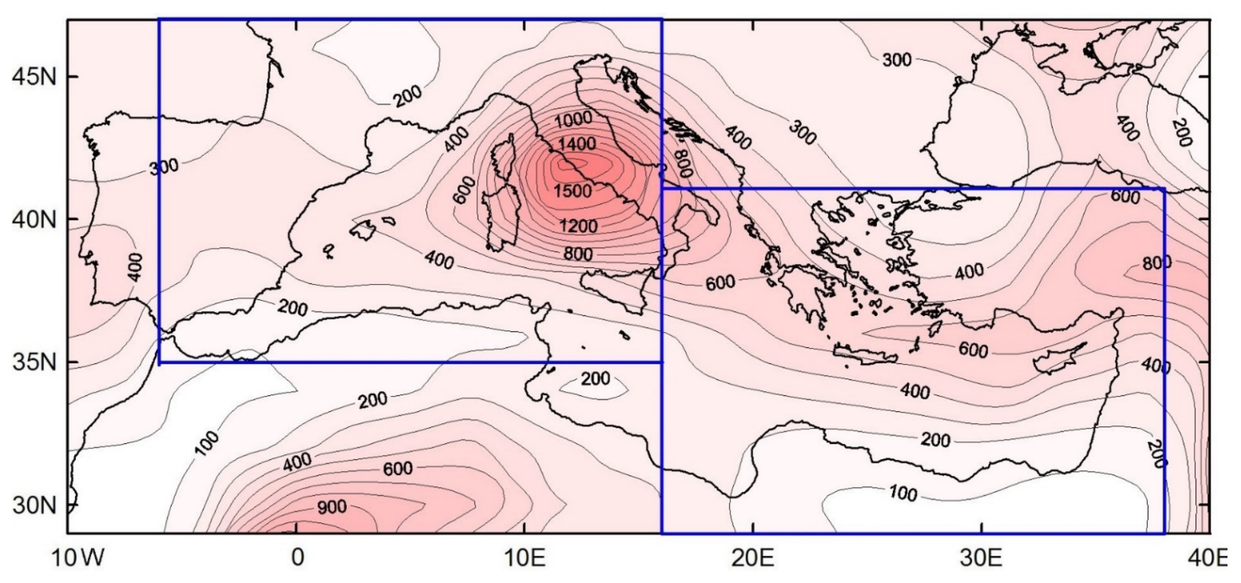
2.2. Cyclone Detection Algorithm

The methodology for identification of cyclones was developed by M.Y. Bardin [70], approved for the Atlantic-European region in [71], and compared with other methods in the international project IMILAST (Intercomparison of Mid Latitude Storm Diagnostic) [72]. The quality control of the methodology, which was performed previously [68], showed a good agreement between the temporal variability of monthly cyclone numbers obtained using NCEP/NCAR reanalysis and composite kinematic maps of the meteorological observations.
A cyclone was identified as a local minimum limited by closed isohypses in the 1000 hPa geopotential height field with a step of 10 gpm. Figure 1 demonstrates the initial results of cyclone identification. It shows the total number of the centers of all identified local minima for the entire period on a 6-h basis in the boxes of 2.5° × 2.5° overlapping each other by 0.5°.
The cyclone area was identified within the external closed isohypse. Cyclone depth was determined as the difference in geopotential heights between the minimum at a grid point within the first closed isohypse and the value on the external closed isohypse. The cyclone intensity (or average depth) was obtained as the ratio of the integral cyclone depth (or geopotential height differences) to the area of the cyclone.
Time series (monthly, seasonal, and annual) of the main parameters of cyclones (the frequency, area, depth, and intensity) were obtained for the Western (35° N–47° N, 6° W–16° E) and Eastern (29° N–41° N, 16° E–38° E) Mediterranean (Figure 1). Due to the extension from west to east and geographical features, the climate of the Mediterranean region is often studied for the western and eastern parts separately, e.g., in [18,73].
The average/minimum/maximum radius of cyclones identified in the reanalysis was 594/138/1734 km for the Western Mediterranean and 563/149/1769 km for the Eastern Mediterranean. The resolution of the NCEP/NCAR reanalysis of 2.5° × 2.5° can underestimate small cyclones but allows the identification of quite large systems, which are most likely associated with the atmospheric circulation patterns and not with one-air-mass processes. Besides, the length of the NCEP/NCAR reanalysis (67 years in this study) is appropriate for the study of temporal variability of climate.
Intense cyclones were obtained by the percentile method, which is often used for calculating extreme meteorological characteristics, e.g., precipitation [8] and storminess [74,75]. Two groups of intense cyclones in the Western and Eastern Mediterranean were obtained by exceeding the thresholds of 75th (≥19.8 gpm and ≥18.6 gpm, respectively) and 95th (≥40.5 gpm and ≥34.95 gpm, respectively) percentiles of the intensity of cyclones. Further, we used the abbreviations WMC-75 and WMC-95 for the groups of intense cyclones in the Western Mediterranean and EMC-75 and EMC-95 for those in the Eastern Mediterranean. The WMC-75 and EMC-75 abbreviations referred to intense cyclones, and the WMC-95 and EMC-95 abbreviations referred to extreme cyclones. It is necessary to note that the variability of cyclones defined as the 75th percentile included the variability of those defined as the 95th percentile.
The relative frequency (or number) of intense and extreme cyclones was defined for each month as the ratio of the number of cyclone centers (of a certain intensity) in the specified region to the total number of timesteps analyzed (equal to the number of days per month multiplied by 4 times because 6-hourly data were used).
As a result, we managed to extract a part of the variability of a certain intensity of cyclones from the variability of the total number of cyclones. Time series of the frequency of cyclones were analyzed in the following terms:
  • Monthly, seasonal, and annual values for the period 1951–2017;
  • Description of fluctuations and analysis of linear trends;
  • Spectral Fourier analysis of seasonal and annual values;
  • Correlation analysis with teleconnection indices;
  • Modeling using our artificial neural network.

2.3. Spectral Analysis

A spectral analysis was carried out to identify the typical periods of variability of the frequency of intense and extreme cyclones in the Mediterranean. Initial time series were not preprocessed (detrended or filtered). As an estimate for the spectrum, we used a periodogram (or the sample spectrum) related to the autocorrelation function and smoothed using the Parzen window [76,77]. Window width (number of lags for autocorrelation function) determines the number of sample autocorrelations used in spectrum estimation, and it was taken as equal to 20 with the number of frequency points equal to 100. This technique is the most effective to increase the number of degrees of freedom, but it reduces the accuracy of determining the peak frequency. Therefore, for a more accurate determination of the peak frequency (or periods in years), we referred to the periods of unsmoothed periodograms.

2.4. Correlation Analysis

Pearson’s correlation analysis (Equation (1)) was performed between the frequency of intense and extreme cyclones and teleconnection indices on the basis of the monthly, seasonal, and annual time series for the period 1951–2017.
r = c o v x , y σ x σ y ,
where r is the correlation coefficient, and σx and σy are the standard deviations of the x and y correlated series.
The significance of the correlation coefficients was identified using the Student’s t-test according to Equation (2):
t = r 2 ( n 2 ) 1 r 2 , 1 < r < 1 ,
where t is the Student’s criterion, r is the correlation coefficient, and n is the length of the time series.
A coefficient of determination (r2) was used to show the proportion of the variance of the frequency of cyclones that was predictable from the correlation with teleconnection indices.
Examples of spatial correlations between teleconnection indices and the 1000 hPa geopotential height were obtained using an online plotting tool of the NOAA Physical Sciences Laboratory available at https://psl.noaa.gov/data/correlation/ (accessed on 13 September 2021), which plots correlations of seasonally averaged variables from the NCEP reanalysis with specified teleconnection and ocean index time series for the 1948–2012 period.

2.5. Description of the Modeling Method

Previously, the modeling using an artificial neural network approach was successfully applied to forecast the frequency of intense cyclones in the Black Sea region [10] and to predict anomalies in the Nino3.4 region with lead times from 1 to 9 months [67].
As already mentioned, the Mediterranean climate is characterized by both decadal-multidecadal (referred to as low-frequency) and interannual (referred to as high-frequency) fluctuations. In this study, the approach used was to decompose the original parameter into the orthogonal signals (low-frequency and high-frequency) with subsequent modeling of each signal separately. As was shown earlier in [67,78], the number of input indexes is limited by computing power, so this approach allowed us to increase the number of predictors (input teleconnection indices) and, consequently, to improve the quality of modeling.
Frequency series of intense cyclones were divided into two components: interannual (or high-frequency) and decadal-multidecadal (or low-frequency), as shown in Figure 2. The original series were smoothed with a 9-year moving filter for each month separately (in order to attribute a ten-year periodicity to the low-frequency one). Both components were modeled independently of each other and summed up after simulation.
To simulate the low-frequency and high-frequency components, we used a unidirectional heteroassociative multilayer neural network model represented by a perceptron with one hidden layer [79,80]. Thus, the neural network model consisted of the input, hidden, and output layers. The neuron activation function was sigmoidal bipolar: f(x) = tanh(βx) [79].
The input parameters were objectively chosen by the model algorithm using spatial correlation analysis between the high-frequency and low-frequency components of the frequency of intense cyclones (taking into account the time lag of their response) and global fields of the following parameters: the 500 hPa geopotential height, wind components, and sea surface temperature for the high-frequency component, and only the sea surface temperature for the low-frequency component. The corresponding centers of maximum correlations are in reference to the atmospheric centers of action [25] and the energy-active zones of the World Ocean [26]. The indices were calculated as average anomalies of the parameters in the regions of significant correlations. In order to ensure comparability, the anomalies were normalized to the variance for the period 1951–2020. The linear trends were excluded for the high-frequency component and saved for the low-frequency component. The indices for the low-frequency component were smoothed with a 9-year moving filter. In total, 55 indices with different lead times were calculated: 29 for the high-frequency components and 26 for the low-frequency components.
The modeling of the components of the frequency of intense cyclones was carried out separately for each month to exclude seasonal variability. The simulation was carried out for three samples of the series: training, testing, and control samples. Earlier studies showed that, for better neural network training, 30-year climatic periods should be taken for testing and training [67,78]. In this study, we used equal 28-year periods: the 1951–1978 period for the training sample and the 1979–2006 period for the testing sample. The 11-year period 2007–2017 was the control period. For the period 2018–(May) 2021, modeling was performed (with a lead time of 6 months) without initial values of cyclones.
The training of the model was based on the error backpropagation algorithm [80]. The goal of training was to determine the values of the weights of the neurons of each layer in such a way that, for a given input parameter, the values of the signals of the output layer (represented by one neuron) coincided with the expected values of the training sample with the required accuracy [79]. In our study, the required accuracy could not be achieved because of the insufficient length of the training sample. In this case, to determine the maximum training, the method described in [79] was used, which was as follows. Correction of the weights of neurons was carried out using the classical objective function, but the training sample was repeated many times, while the weight values were saved. At each iteration of the training, the correlation coefficients with the training (rstudy) and test (rtest) samples were calculated. The training maximum had to satisfy 2 conditions: determining the iteration of the training with the maximum rstudy and the inequality |rstudyrtest| <0.15 had to be satisfied. If the second condition was not fulfilled, the closest iteration corresponding to both conditions was taken as the maximum training. Since a test sample was used in the search for the training maximum, it was necessary to use an independent control sample for an objective assessment of the model capabilities.
The adaptation of the model was carried out following the algorithm in [67,78] and included the stages of preprocessing, modeling, and postprocessing.
At the stage of preliminary data processing, a search was made for the correlation between the input indices and the components of the frequency of intense cyclones with the lead time from one month to two years for the high-frequency component and from one to ten years for the low-frequency component. The inputs for the operation of the model were selected as the indices that had the maximum correlation with the frequency of cyclones. Since an increase in the number of input parameters significantly affects the calculation speed, no more than 22 and 16 input indices were used to simulate the high-frequency and low-frequency components, respectively. The modeling was carried out many times with different combinations (changing the number) of the inputs selected at the preliminary stage and changing the number of neurons in the hidden layer, as was done previously in [78]. At the final stage, the best 20 neural network combinations were selected based on the ranking of correlation coefficients for a testing sample. Then, their ensemble was calculated. The quality of calculation was estimated in comparison with the control sample. For this assessment, we used Pearson’s correlation coefficient (Equation (2)), the standard deviation of the model values relative to the original values (root mean square error, RMSE) (Equation (3)), as well as the standardized RMSE (normalized to standard deviation of the original series σ) to ensure comparability of results for different months (RMSE/σ):
RMSE = x i y i 2 n ,
where x and y are the samples that represent the simulation result and the original series, and n is the length of the control sample series.

3. Results

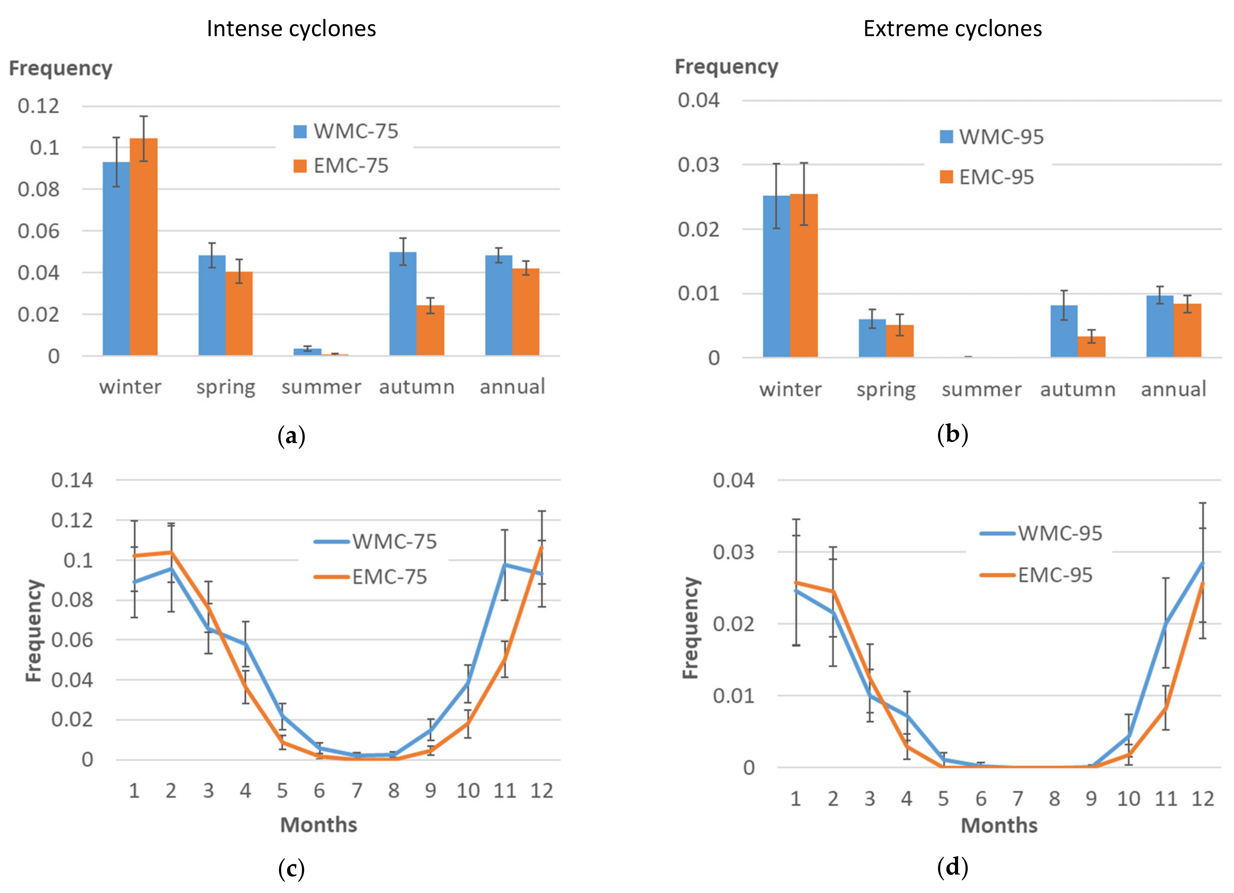
3.1. Seasonal and Monthly Averages

The annual frequency of intense and extreme cyclones was higher in the Western Mediterranean, as was the case in spring and autumn (Figure 3a,b). However, the frequency of intense cyclones was higher in the Eastern Mediterranean in the winter season (Figure 3a) and from December to March (Figure 3c). The frequency of extreme cyclones in winter was almost equal in the two regions of the Mediterranean (Figure 3b) and a little higher in the Eastern Mediterranean from January to March (Figure 3d). Summer averages were negligible (Figure 3a,b). Monthly averages were close to zero for intense cyclones in June–August (Figure 3c) and for extreme cyclones in May–September (Figure 3d). The highest monthly frequency of intense cyclones (Figure 3c) was in November for the Western Mediterranean and in December for the Eastern Mediterranean. The highest monthly frequency of extreme cyclones for both the Western and Eastern Mediterranean (Figure 3d) was in December (and also in January for the Eastern Mediterranean).

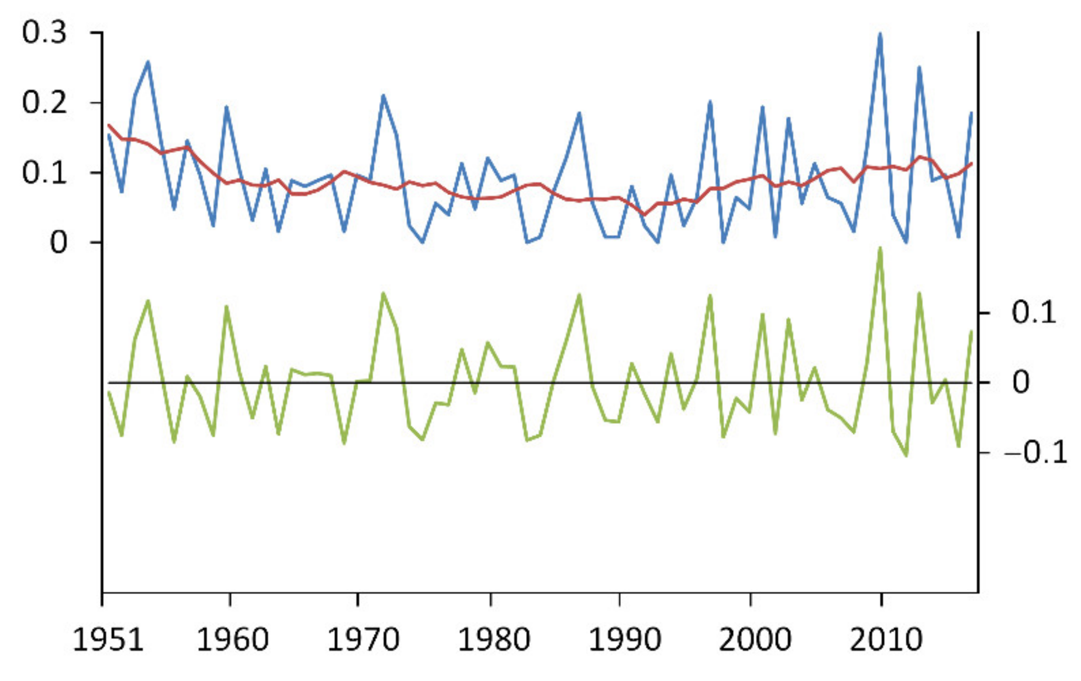
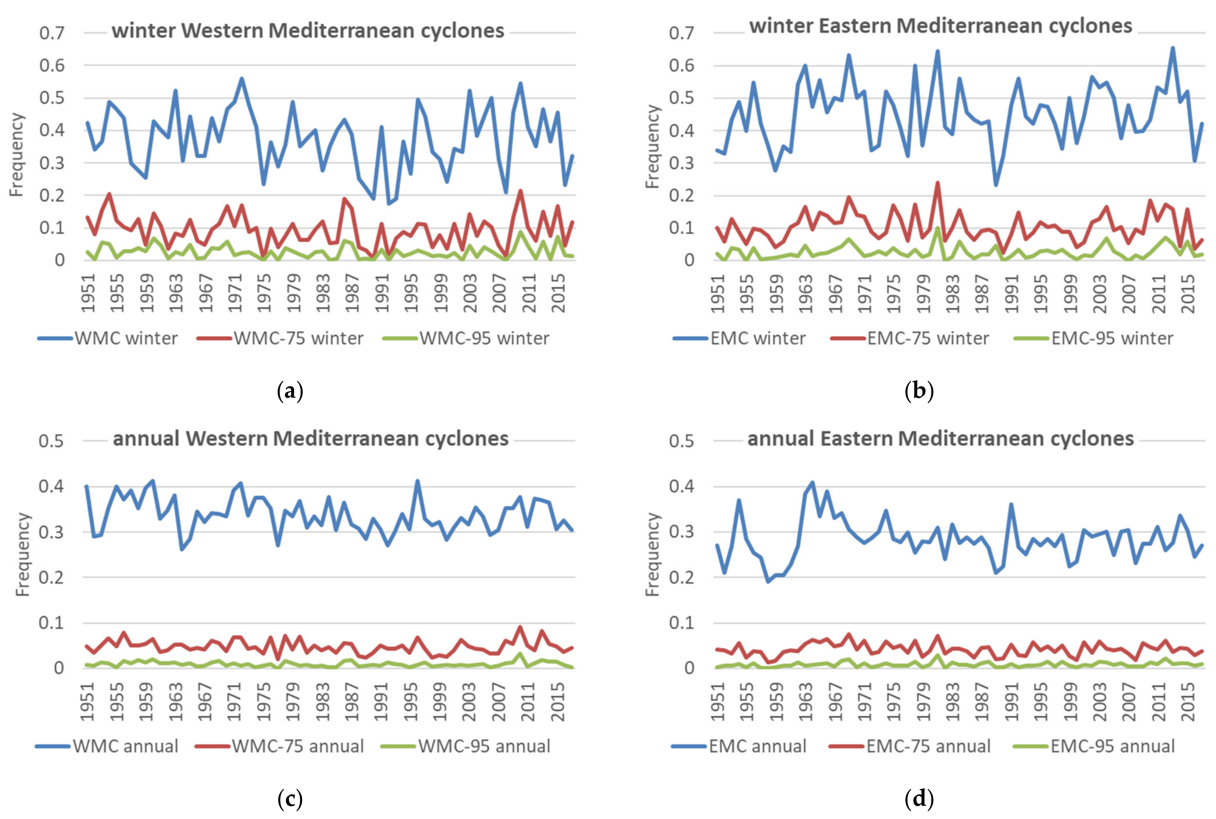
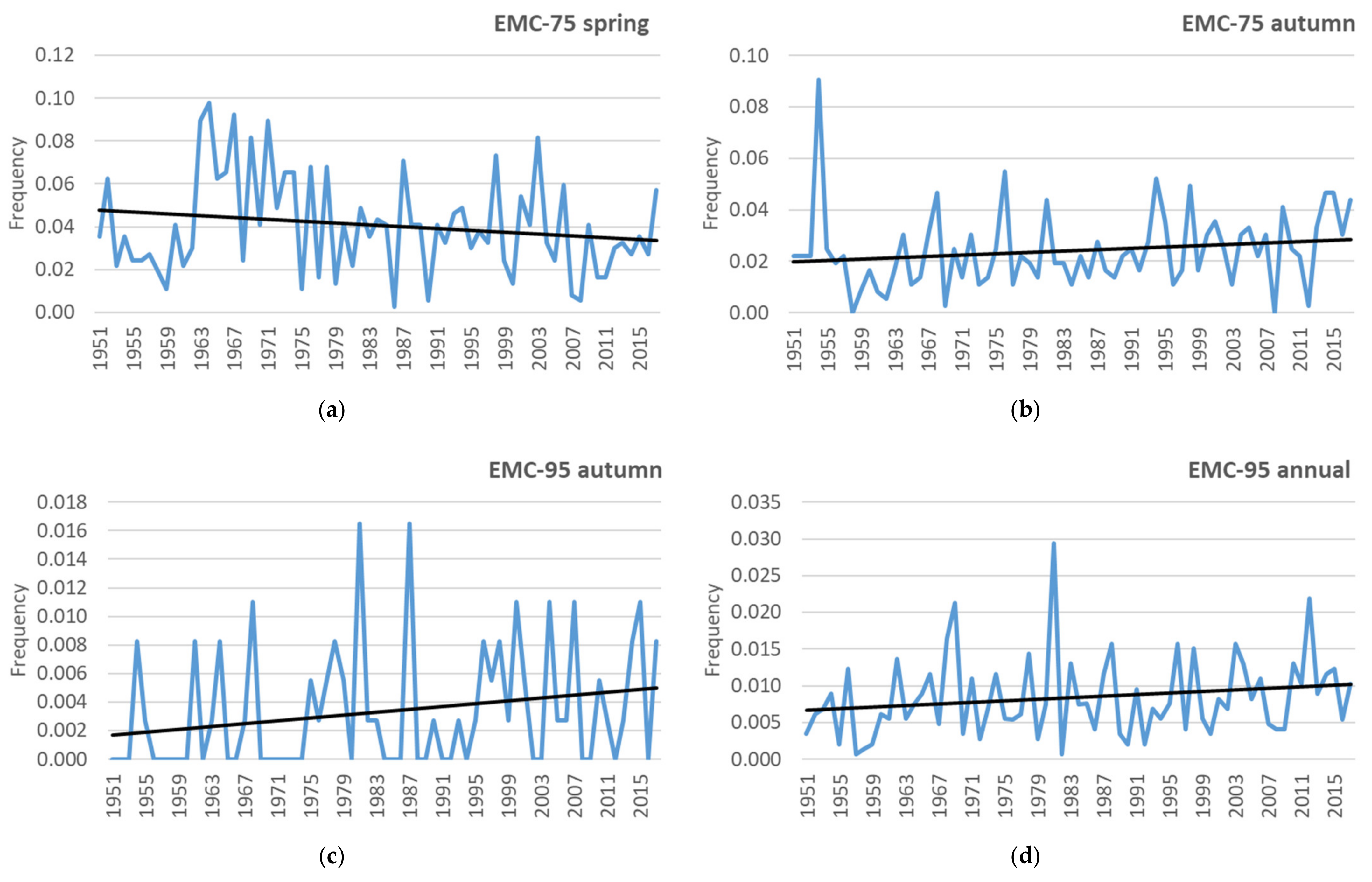
3.2. Variability and Linear Trends

Figure 4 shows annual and winter time series for the frequency of the total number of cyclones, and numbers of intense and extreme cyclones in the Western and Eastern Mediterranean. All series of cyclones in both regions of the Mediterranean were characterized by a pronounced interannual variability. At the same time, there were noticeable differences for the Western and Eastern Mediterranean. For example, from about 1955 to 1965, the interannual variability in the annual frequency of the total number of cyclones in the Eastern Mediterranean was not pronounced, but instead there was a decline and then an increase, which could be part of the decadal variability (Figure 4d). Similar episodes can be seen in other periods of annual cyclones, including the Western Mediterranean cyclones (Figure 4c), but the quasidecadal variability was better expressed in the series of winter cyclone numbers, total and intense, in both regions of the Mediterranean (Figure 4a,b).
According to Table 1, there were no significant linear trends for the Western Mediterranean cyclones. For the Eastern Mediterranean cyclones, there was a negative linear trend for spring intense cyclones (at the 85% confidence level), and there were positive trends for autumn intense and extreme cyclones (at the 80% and 90% confidence levels, respectively), as well as for annual extreme cyclones (at the 85% confidence level). The contribution of these significant linear trends to the variance of the series was 3–5%.
To illustrate the series with significant linear trends for the Eastern Mediterranean, Figure 5 shows the time plots of the frequency of spring and autumn intense cyclones (Figure 5a,b) and the frequency of autumn and annual extreme cyclones (Figure 5c,d).
Linear trends of the 67-year series can be interpreted both as manifestations of the global temperature rise, and as part of a lower-frequency variability with periods comparable to or exceeding the length of the series. Actually, any climate series is the result of both factors, and the problem of separating the anthropogenic and natural components of climate change and variability has not been solved yet. As the natural factors, we consider 60–80-year climate variability associated with the multidecadal processes in the North Atlantic and North Pacific (AMO and PDO). As for the global temperature rise, there are regional features, and regional climate anomalies may not correspond to the global trend [81]. For example, Figure 6 shows spatial correlations between global temperature and 1000 hPa geopotential height over Europe for seasonal and annual series. According to Figure 6, the correlation coefficients were higher over the Eastern Mediterranean than over the Western Mediterranean. This may be explained by the decreasing influence of the ocean (from west to east) that engulfs the surface temperature rise [82] and by the increasing influence of the continents over which the maximum temperature rise is observed [81].
Figure 6c shows that spring was characterized by the highest correlation coefficients over the entire Mediterranean region (r ≥ +0.4) between global temperature and 1000 hPa geopotential height. At the same time, there was a significant negative trend in the frequency of intense cyclones in spring over the Eastern Mediterranean. This can be explained by the greater contribution of natural variability of a multidecadal scale in spring.

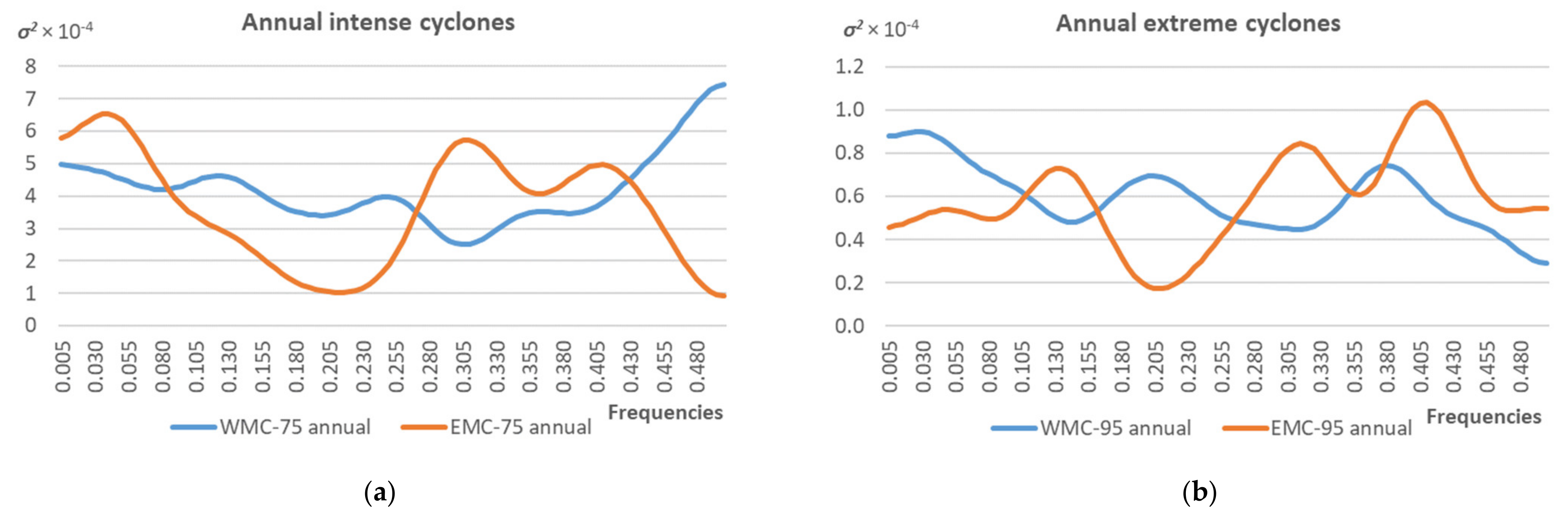
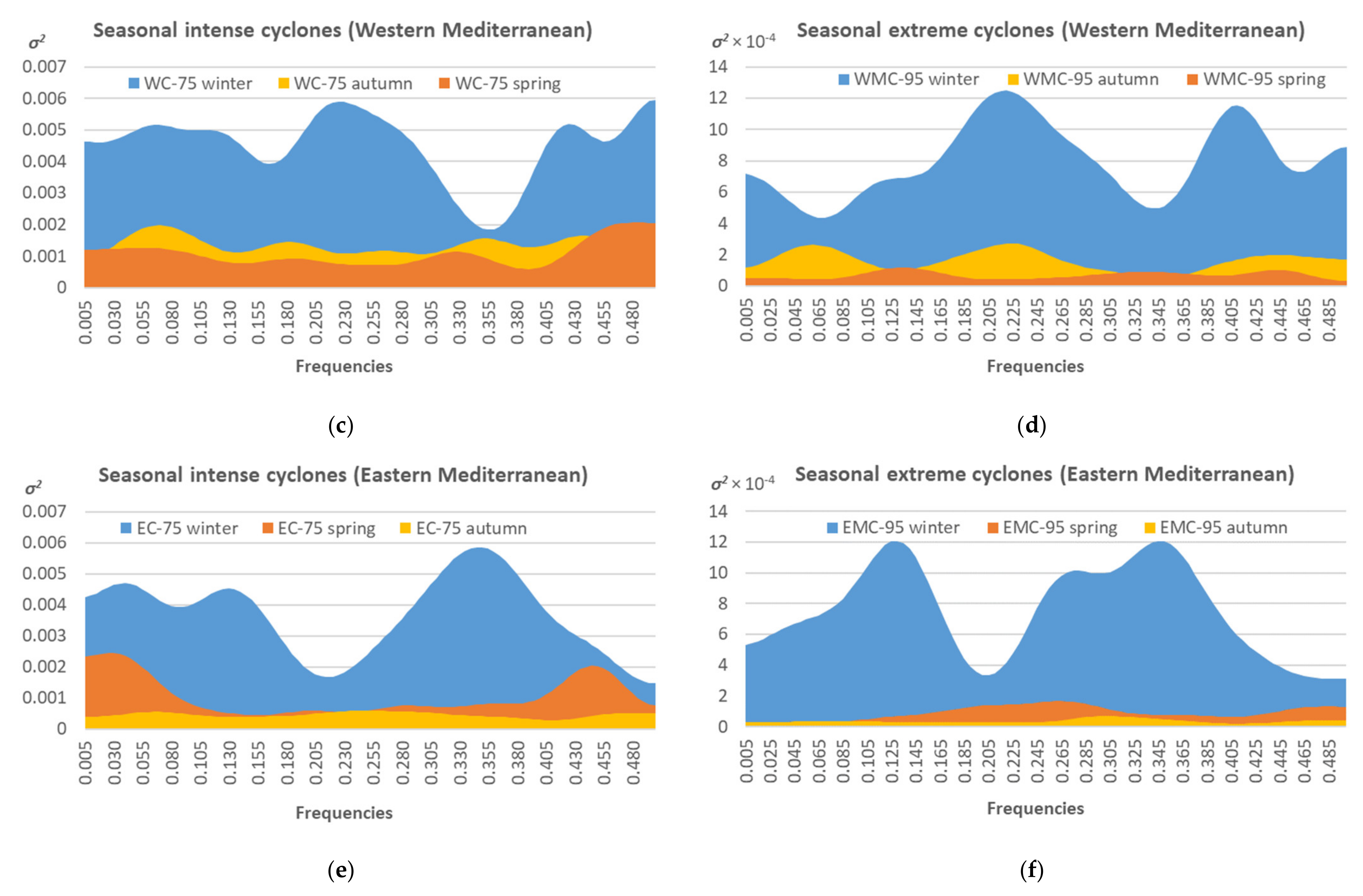
3.3. Spectral Analysis

Figure 7 shows smoothed periodograms of the annual and seasonal (except summer) intense and extreme cyclones in the Eastern and Western Mediterranean, and Table 2 contains periods of the Fourier decomposition that contribute at least 8% to the dispersion of the series and are significant at the 75% confidence level.
Annual spectra of intense and extreme cyclones over the Eastern Mediterranean had higher levels of energy at peaks of about 2–2.5 years (0.305–0.405 units of spectral frequencies) compared with those over the Western Mediterranean and lower levels of energy at peaks of about 3 years (0.205 units of spectral frequency) (Figure 7a,b). As for the seasons, most of the energy was concentrated in winter spectra (Figure 7c–f); spring and autumn were characterized by comparable levels of energy, a little higher in autumn for the Western Mediterranean (Figure 7c,d) and in spring for the Eastern Mediterranean (Figure 7e,f).
According to Table 2, for the Western Mediterranean, significant spectral maxima of the annual series were at about 4 and 8 years for intense cyclones and at about 2.5 for extreme cyclones. For the Eastern Mediterranean, the annual frequencies of intense and extreme cyclones were characterized by spectral peaks at about 3.5 years for intense cyclones and about 2.5 and 8 years for extreme cyclones. The periods of about 8 years in annual spectra were due to the contribution of winter spectra. A period of about 2–3 years occurred in most seasons. Periods of about 4.5 and 7.5 years were obtained for the seasonal series of extreme cyclones over the Western and Eastern Mediterranean.
The spectral periods obtained for intense and extreme Mediterranean cyclones correspond to the typical spectral periods of the main global climate processes: 2.4, 4.8, and 7.7 years for the winter NAO index [83], and 3–4 and 7–8 years for the ENSO [84]. The results showed that, in the spectra of both groups of intense cyclones, for the Eastern Mediterranean, there was more energy in the interannual periods (about 2.5 years) coinciding with the NAO period; for the western Mediterranean, there was more energy in the periods (about 3 years) corresponding to the ENSO periods. On the one hand, geopotential height/sea level pressure depends more on the NAO over the Western Mediterranean, and more likely on the ENSO over the Eastern Mediterranean through the influence of the Asian monsoon [85]. On the other hand, it should be remembered that results of spectral analysis show the relative energy of the peaks (compared with the contribution of peaks of other periodicities). Over the Western Mediterranean, the main cyclogenesis occurs, which can lead to a wider range of periodicities in the spectra. Over the Eastern Mediterranean, cyclones often reach a mature stage, which can increase the contribution to the spectra from cyclones caused by large-scale patterns over the North Atlantic. It should also be taken into account that this study is focused on the frequency of intense cyclones. In this case, the possible influence of NAO and ENSO can manifest differently in the frequency and in the depth (intensity) of cyclones.

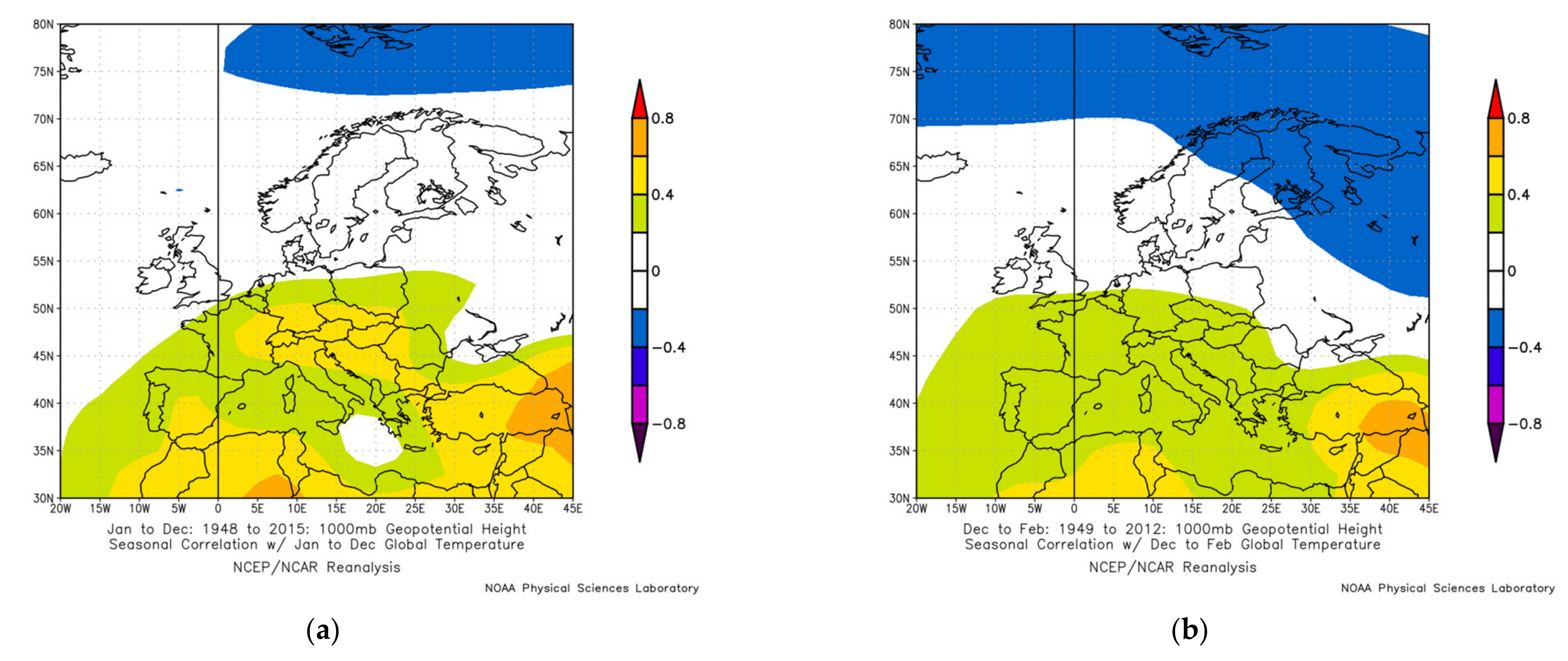
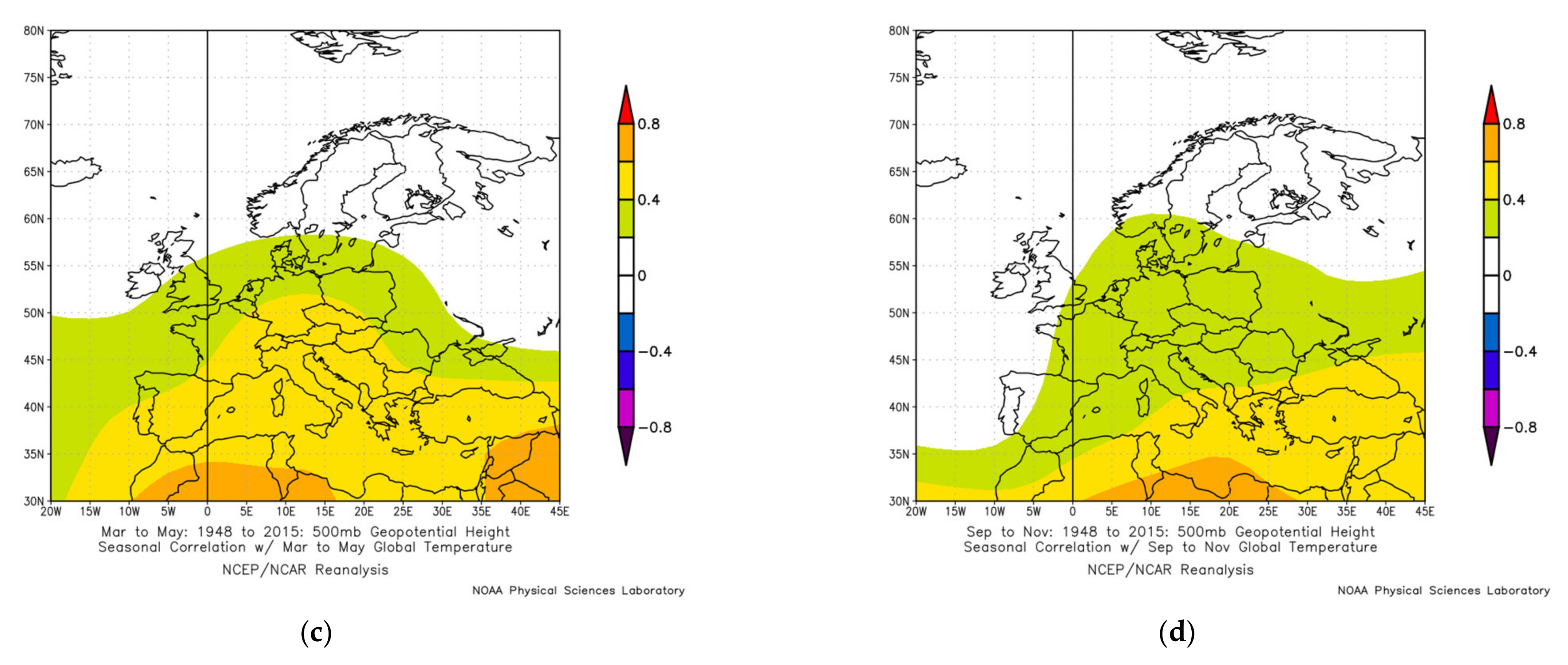
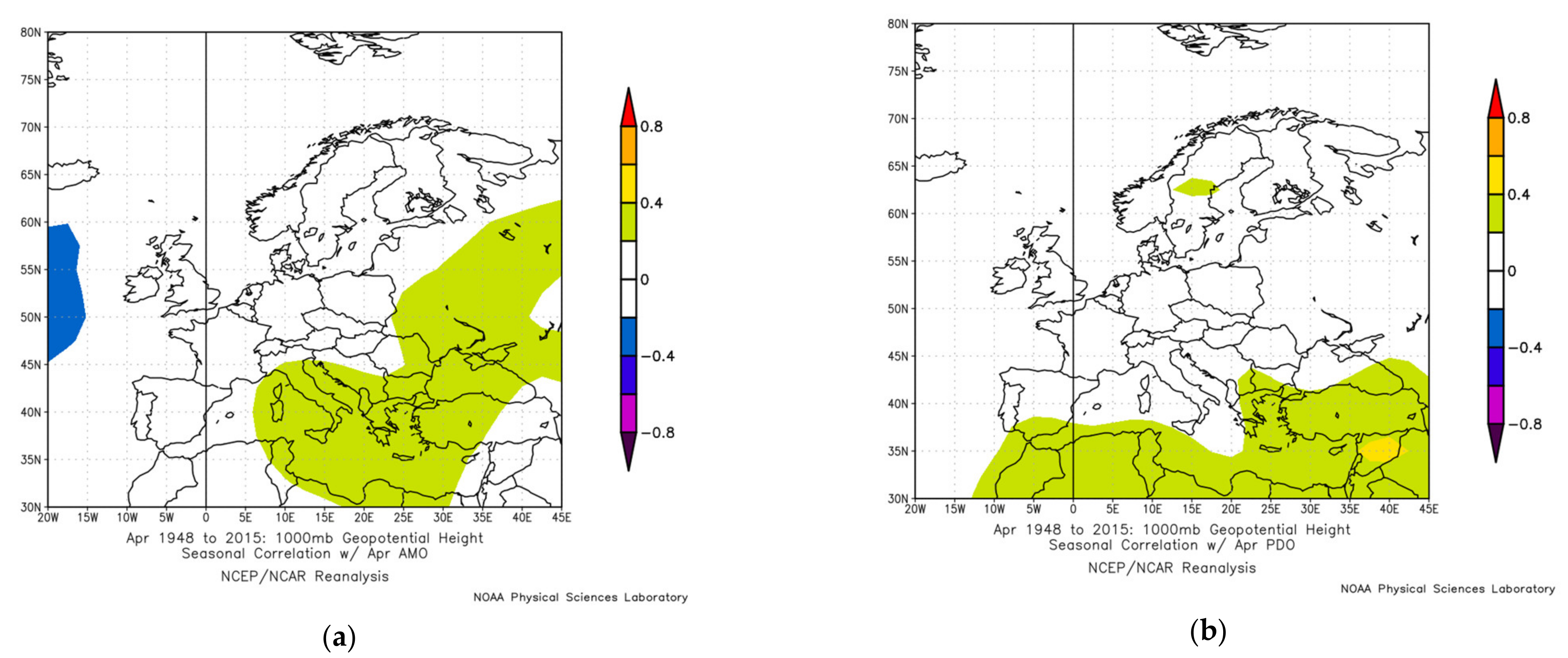
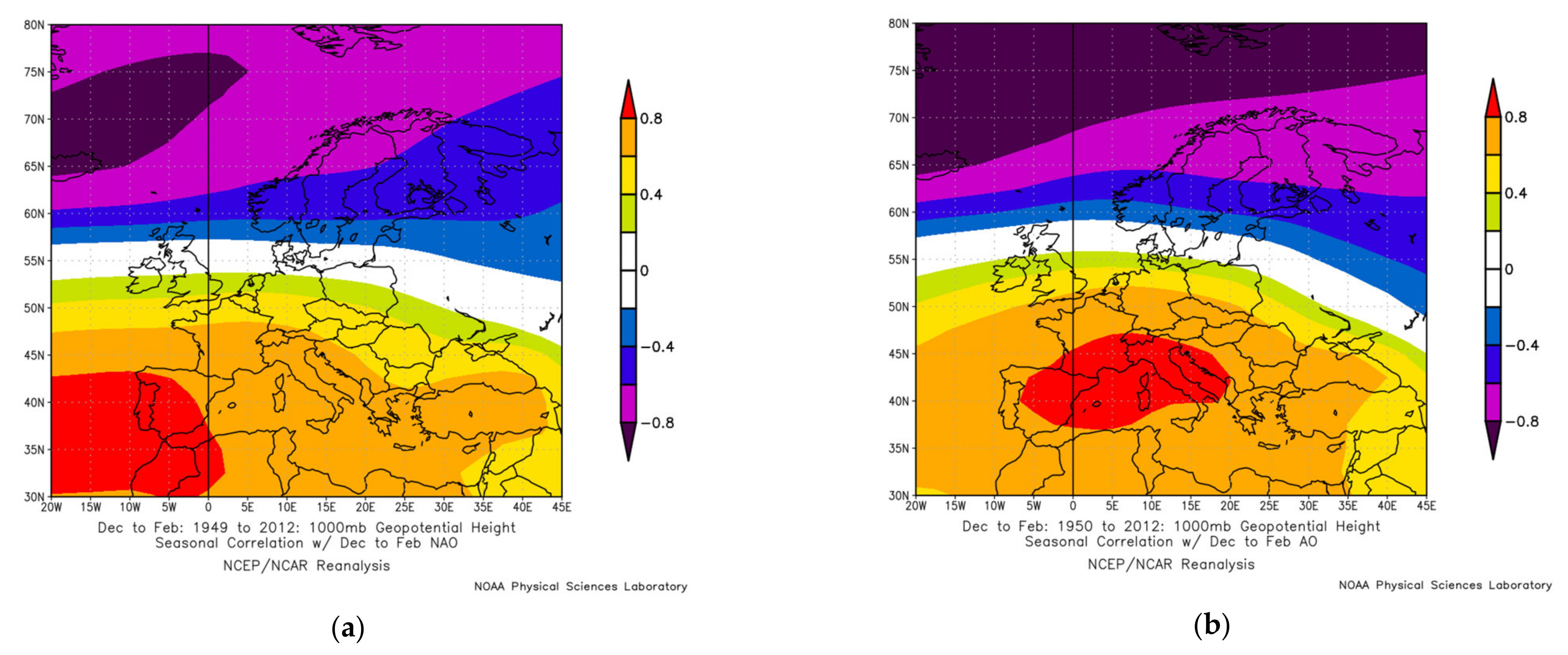
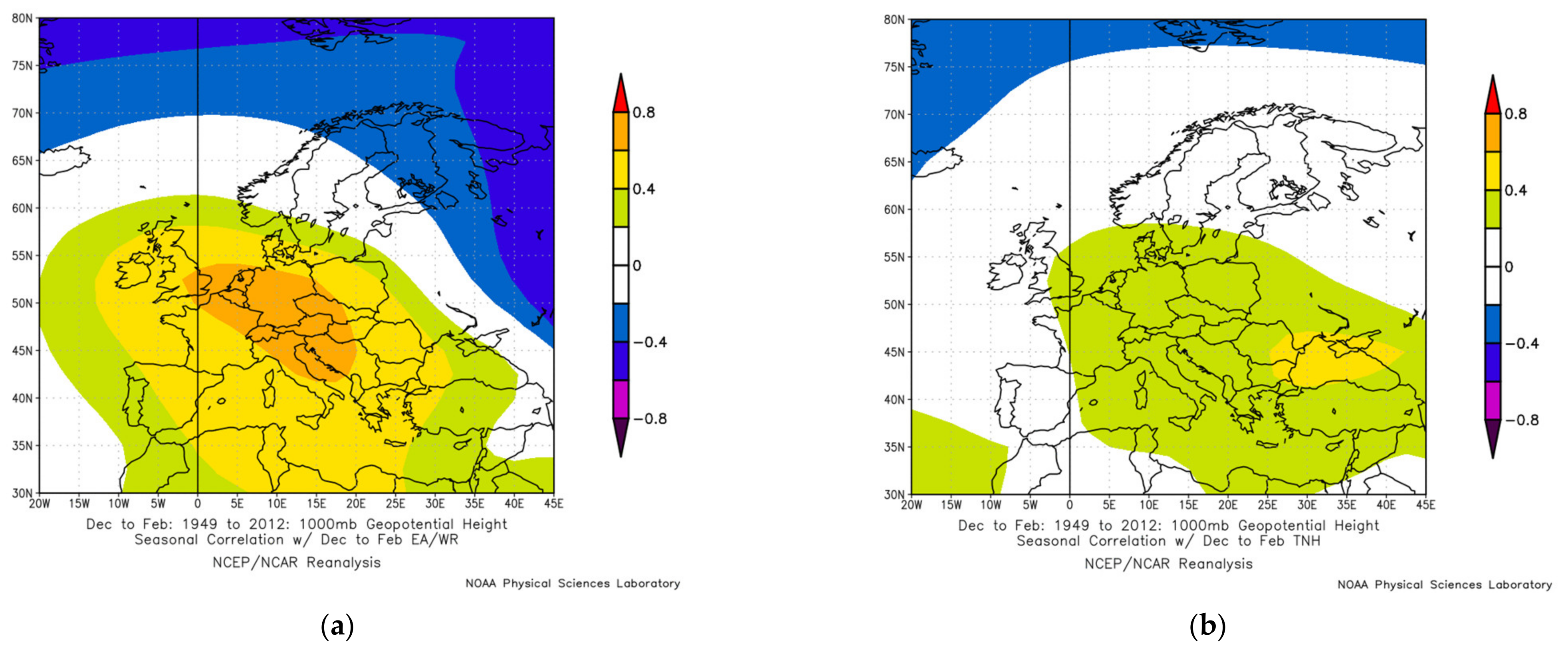
3.4. Correlation with Teleconnection Patterns

Correlation analysis was performed between the frequency of intense and extreme cyclones and teleconnection indices on the basis of the monthly, seasonal, and annual time series for the 1951–2017 period. Further, we described significant correlations (r ≤ −0.3 and r ≥ +0.3) with teleconnection indices that contribute at least r2 = 9% to the variance of cyclones. Correlation coefficients (r) significant at the 90% confidence level were r < −0.2 and r > +0.2. Additionally, to illustrate how teleconnection patterns influence large-scale atmospheric circulation over Europe, spatial correlations were obtained between the 1000 hPa geopotential height and some teleconnection indices. Correlations were shown mostly for the winter season when atmospheric gradients are increased over the Northern Hemisphere.
Annual series of intense cyclones in the Western Mediterranean (WM) correlated with the following indices of the teleconnection patterns:
  • annual SCAND (+0.35);
  • winter SCAND (+0.28) mostly due to February SCAND (+0.37);
  • spring SCAND (+0.28);
  • winter NAO (−0.38) mostly due to February NAO index (−0.34);
  • winter AO (−0.34) mostly due to February AO index (−0.32);
  • February MO index (−0.34);
  • September AO index (−0.34);
  • April EA index (−0.3).
Winter series of intense cyclones in the Western Mediterranean correlated with the following indices of the teleconnection patterns:
  • winter MO (−0.45);
  • winter AO (−0.44) mostly due to February AO (−0.43);
  • annual AO (−0.31);
  • winter SCAND (+0.39) mostly due to February SCAND (+0.35);
  • May POL/EUR (−0,36);
  • May WMO (+0.33);
  • winter NAO (−0.27) mostly due to February NAO (−0.3);
  • May SOI (−0.27).
Spring series of intense cyclones in the Western Mediterranean correlated with the following indices of the teleconnection patterns:
  • spring SCAND (+0.41) mostly due to March SCAND (+0.34);
  • annual SCAND (+0.35);
  • spring SOI (+0.33) mostly due to March SOI (+0.31);
  • December TNH index (+0.32);
  • autumn ER/WR (+0.32);
  • autumn NAO (+0.31);
  • spring AMO (−0.44) due to March AMO (−0.4), April AMO (−0.43), and May AMO (−0.44);
  • spring EA (−0.39) due to April EA (−0.36) and May EA (−0.33);
  • spring MO (−0.36) due to March MO (−0.36);
  • annual EA (−0.32) and August EA (−0.34);
  • February WMO index (−0.31);
  • summer AMO (−0.49) due to June AMO (−0.51), July AMO (−0.48), and August (−0.44) AMO;
  • autumn AMO (−0.44) due to September AMO (−0.44), October AMO (−0.4), and November AMO (−0.45);
  • annual AMO (−0.46) and December AMO (−0.51);
  • winter WP (−0.36) mostly due to January WP (−0.4);
  • summer PNA (−0.3) mostly due to July (−0.3).
Summer series of intense cyclones in the Western Mediterranean correlated with the following indices of the teleconnection patterns:
  • summer WMO (+0.3) mostly due to August WMO (+0.33);
  • annual WMO (+0.35);
  • annual POL/EUR index (+0.3);
  • annual NAO (−0.46);
  • winter NAO (−0.44) due to December NAO (−0.33), January NAO (−0.34), and February NAO (−0.34);
  • spring NAO (−0.35);
  • annual AO (−0.39) and April AO (−0.35);
  • winter AO (−0.39) mostly due to December AO (−0.3) and January AO (−0.32);
  • December TNH (−0.39).
June intense cyclones in the Western Mediterranean positively correlated with April and spring AMO indices (+0.26–+0.3), and July cyclones positively correlated with seasonal and monthly PDO indices for spring and summer (+0.3–+0.37).
Autumn series of intense cyclones in the Western Mediterranean correlated with the following indices of the teleconnection patterns:
  • November EP/NP index (+0.3);
  • November MO index (−0.43);
  • winter WMO (−0.31) mostly due to February (−0.35);
  • December PNA index (−0.35).
September intense cyclones in the Western Mediterranean positively correlated with August SCAND index (+0.32), and October cyclones positively correlated with winter POL/EUR index (+0.35).
Annual series of intense cyclones in the Eastern Mediterranean (EM) correlated with the following indices of the teleconnection patterns:
  • annual MO (+0.28);
  • winter AO (−0.3) mostly due to January AO (−0.34);
  • December TNH (−0.43).
Winter series of intense cyclones in the Eastern Mediterranean correlated with the following indices of the teleconnection patterns:
  • winter MO (+0.32) due to January MO (+0.33);
  • winter EA (−0.33);
  • winter TNH (−0.31);
  • winter WP (−0.29) due to January WP index (−0.37).
Monthly synchronous correlation (correlation between cyclones and indices in the same month) reached, with MO index, +0.48 in January and +0.52 in December; and with SCAND index, +0.33 in February.
Spring series of intense cyclones in the Eastern Mediterranean correlated with the following indices of the teleconnection patterns:
  • spring SCAND (+0.33);
  • March MO (+0.33);
  • June EA/WR (+0.3);
  • spring WP (+0.32) due to April WP (+0.41) and May WP (+0.3);
  • annual WP (+0.29);
  • winter EA (−0.31);
  • May PNA (−0.35).
Monthly synchronous correlation with MO index reached +0.47 in March.
April intense cyclones in the Eastern Mediterranean correlated with the following indices of the teleconnection patterns:
  • annual SCAND (+0.35) and February SCAND (+0.32);
  • summer EA/WR (+0.36) due to June EA/WR (+0.35);
  • August EP/NP (+0.35);
  • autumn EP/NP (+0.3) due to September EP/NP (+0.38);
  • monthly AMO indices (−0.5–−0.55);
  • April EA (−0.44);
  • March PNA (−0.33);
  • May PDO (−0.32).
Summer series of intense cyclones in the Eastern Mediterranean, represented only by June and August cyclones, negatively correlated with August NAO (−0.3) and AO (−0.29) indices and positively correlated with November EP/NP index (0.34).
Autumn series of intense cyclones in the Eastern Mediterranean correlated with the following indices of the teleconnection patterns:
  • autumn MO (+0.27) due to November MO (+0.43 with autumn cyclones and +0.5 with November cyclones);
  • September WMO (+0.33);
  • September NAO (−0.3 with November cyclones);
  • August EA/WR (−0.27);
  • April SCAND (−0.3).
Annual series of extreme cyclones in the Western Mediterranean correlated with the following indices of the teleconnection patterns:
  • annual AO (−0.32);
  • winter AO (−0.34) mostly due to February AO (−0.37);
  • winter NAO (−0.33) mostly due to February NAO (−0.38);
  • March EA/RW (+0.34).
Winter series of extreme cyclones in the Western Mediterranean correlated with the following indices of the teleconnection patterns:
  • winter AO (−0.44) mostly due to February AO (−0.37);
  • winter NAO (−0.3) mostly due to February NAO (−0.35);
  • winter MO (−0.33);
  • May POL/EUR (−0.34);
  • May EA/WR (−0.3).
Monthly synchronous correlation reached, in December, −0.38 with EA/WR index and −0.36 with MO index; and in February, −0.35 with MO, −0.36 with SOI, and −0.38 with AO.
Spring series of extreme cyclones in the Western Mediterranean correlated with the following indices of the teleconnection patterns:
  • April MO index (−0.33);
  • March PDO (−0.31);
  • winter PDO (−0.4) due to January PDO (−0.38) and February PDO (−0.38);
  • January AO index (+0.37).
Summer series of extreme cyclones in the Western Mediterranean, represented only by June cyclones, positively correlated with June EP/NP index (+0.34) and negatively correlated with May SOI index (−0.32).
Autumn series of extreme cyclones in the Western Mediterranean correlated with the following indices of the teleconnection patterns:
  • November MO (−0.38);
  • June WMO index (+0.34);
  • autumn WMO index (+0.32 with October cyclones).
Annual series of extreme cyclones in the Eastern Mediterranean correlated with the following indices of the teleconnection patterns:
  • January MO (+0.39);
  • autumn NAO index (−0.33);
  • winter TNH (−0.31) mostly due to January TNH (−0.31);
  • June WMO (−0.3);
  • August WP (−0.3).
Winter series of extreme cyclones in the Eastern Mediterranean correlated with the following indices of the teleconnection patterns:
  • January MO (+0.42);
  • January WP index (−0.36).
Monthly synchronous correlation reached:
  • in January, +0.5 with MO index, +0.27 with PNA index, and +0.26 with WMO index;
  • in December, +0.39 with MO index, −0.3 with TNH index, and −0.26 with EA index;
  • in February, −0.5 with EA index and +0.28 with SCAND index.
Spring series of extreme cyclones in the Eastern Mediterranean, represented only by March and April cyclones, correlated with the following indices of the teleconnection patterns:
  • winter EA/WR index (+0.32);
  • winter EA/WR index (+0.32);
  • autumn NAO (−0.3) due to September NAO (−0.43);
  • summer SCAND (−0.34).
April cyclones featured negative correlations with monthly PNA and PDO indices (−0.25–−0.39), and also with synchronous POL/EUR index (−0.35).
Autumn series of extreme cyclones in the Eastern Mediterranean, represented only by October and November cyclones, correlated with the following indices of the teleconnection patterns:
  • autumn MO index (+0.32);
  • July MO index (−0.29);
  • April EA/WR index (+0.42);
  • October EA/WR index (−0.39);
  • September WP (+0.33);
  • winter PNA (+0.33) mostly due to February PNA (+0.32);
  • spring PDO (+0.3) mostly due to March PDO (+0.33);
  • September EP/NP (−0.31).
Generalizing the results, for the Western Mediterranean cyclones mostly in the cold half-year months, the main synchronous teleconnections (the same month for cyclones and indices) with positive correlations were:
  • Scandinavia pattern in January (+0.25 for intense cyclones), February (+0.35 for intense cyclones), March (+0.37 for intense cyclones), April (+0.31 for intense cyclones and +0.26 for extreme cyclones), and September (+0.2 for intense cyclones);
and the main synchronous regional teleconnections with negative correlations were:
  • Mediterranean Oscillation in September (−0.26 for intense cyclones), October (−0.43 for intense cyclones and −0.33 for extreme cyclones), November (−0.49 for intense cyclones and −0.41 for extreme cyclones), December (−0.42 for intense cyclones and −0.36 for extreme cyclones), January (−0.27 for intense cyclones), February (−0.44 for intense cyclones and −0.35 for extreme cyclones), March (−0.45 for intense cyclones and −0.31 for extreme cyclones), April (−0.29 for intense cyclones and −0.34 for extreme cyclones), and even May (−0.48 for intense cyclones and −0.21 for extreme cyclones);
  • East Atlantic Oscillation in October (−0.36 for intense cyclones and −0.24 for extreme cyclones), November (−0.28 for intense cyclones), December (−0.33 for intense cyclones), February (−0.22 for intense cyclones), April (−0.29 for intense cyclones), and May (−0.42 for intense cyclones);
  • Arctic Oscillation in January (−0.21 for extreme cyclones), February (−0.33 for intense cyclones and −0.38 for extreme cyclones), September (−0.26 for intense cyclones), October (−0.26 for intense cyclones), and December (−0.28 for intense cyclones and −0.27 for extreme cyclones);
  • East Atlantic/West Russia pattern in December (−0.38 for extreme cyclones).
For the Eastern Mediterranean cyclones mostly in the cold half-year months, the main synchronous teleconnections with positive correlations were:
  • Mediterranean Oscillation in November (+0.5 for intense cyclones and +0.28 for extreme cyclones), December (+0.52 for intense cyclones and +0.39 for extreme cyclones), January (+0.48 for intense cyclones and +0.5 for extreme cyclones), and March (+0.47 for intense cyclones and +0.3 for extreme cyclones);
  • Scandinavia pattern in February (+0.33 for intense cyclones and +0.28 for extreme cyclones);
and the main synchronous regional teleconnections with negative correlations were:
  • East Atlantic Oscillation in January (−0.33 for intense cyclones), February (−0.36 for intense cyclones and −0.5 for extreme cyclones), and April (−0.44 for intense cyclones);
  • Tropical Northern Hemisphere in December (−0.37 for intense cyclones and −0.3 for extreme cyclones);
  • Polar/Eurasia pattern in February (−0.27 for intense cyclones), April (−0.35 for extreme cyclones), and October (−0.23 for extreme cyclones).
For the months from May to August, the main synchronous correlations were with the following teleconnection patterns:
  • Arctic Oscillation in July (+0.26 for the WM intense cyclones);
  • Western Mediterranean Oscillation in August (+0.21 for the WM intense cyclones) and September (+0.2 for the WM intense cyclones);
  • East Atlantic/West Russia pattern in July (+0.21 for the WM intense cyclones);
  • Atlantic Multidecadal Oscillation in August (−0.22 for the WM intense cyclones) and September (+0.27 for intense EM cyclones);
  • Polar/Eurasia pattern in June (−0.2 for the WM extreme cyclones);
  • North Atlantic Oscillation in August (−0.2 for the EM intense cyclones).
Analyzing the results of the correlation analysis, first of all, we should pay attention to the April cyclones, which featured the strongest correlation with teleconnection indices. Both in the Western and Eastern Mediterranean, April intense cyclones negatively correlated with AMO indices (most strongly with May and July indices, r = −0.55), and April extreme cyclones negatively correlated with PDO indices (most strongly with February index, r = −0.4). This can be attributed to a substantial part of decadal-multidecadal variability in the series of April cyclones. The contribution of the decadal periodicities (≥10 years) was about 20% for the April extreme cyclones in the Mediterranean region and reached 28% and 48% for intense cyclones, respectively, in the Western and Eastern Mediterranean.
To illustrate spatial manifestations of the AMO and PDO in the 1000 hPa geopotential height in April, Figure 8 shows the maps of their linear correlations. Significant correlations with the AMO index were over the central part of the Mediterranean Sea and Eastern Europe and with the PDO index were over the east and south of the Mediterranean region.
As for the seasons, in spring, correlations with AMO and PDO appeared only for the Western Mediterranean cyclones: −0.44 for intense cyclones with spring AMO index and −0.4 for extreme cyclones with winter PDO index. A positive correlation with PDO was also found in July for intense cyclones in the Western Mediterranean (+0.35 with May PDO index and +0.36 with June PDO index).
For the Western Mediterranean cyclones, January stands out among the winter months with relatively weaker synchronous correlations with regional monthly teleconnections and stronger correlations with winter indices and multidecadal oscillations, such as the AMO.
Further, we analyzed the results from the point of view of teleconnection patterns.
The NAO was not the main synchronous teleconnection pattern for the deep cyclones in the Mediterranean. Its strongest synchronous correlations were −0.3 with the December WM intense cyclones, −0.28 with the February WM extreme cyclones, and −0.26 with the February EM intense and extreme cyclones.
Figure 9a,b illustrates that spatial correlations of the 1000 hPa geopotential height in winter were higher with the AO index than with the NAO index over the west and north of the Mediterranean.
Although AO and NAO are related signals, the Arctic Oscillation synchronously (in the same month of the cyclone and index series) manifested in winter months better for both groups of intense Mediterranean cyclones than the North Atlantic Oscillation, but their asynchronous manifestations were similar (when the month of the index series precedes the month of the cyclone series).
Asynchronous correlation with the NAO reached:
  • −0.37 for the November EM intense cyclones with September index (a 2-month lag of cyclones);
  • −0.21 for the March WM intense cyclones with January index (a 2-month lag);
  • +0.27 for the April WM intense and extreme cyclones with January index (a 3-month lag);
  • −0.36 for the June WM intense cyclones with January index (a 5-month lag) and −0.34 with December index (a 6-month lag).
Asynchronous correlation with AO reached:
  • +0.27 and +0.39 for April WM intense and extreme cyclones, respectively, with January index (a 3-month lag of cyclones);
  • +0.24 for March WM intense cyclones with December index (a 3-month lag);
  • +0.34 for February WM extreme cyclones with November index (a 3-month lag);
  • −0.33 for November WM extreme cyclones with July index (a 4-month lag);
  • −0.34 for June WM intense cyclones with January index (a 5-month lag);
  • −0.32 for the May WM intense cyclones with September index (an 8-month lag).
For January cyclones, there was a correlation with February NAO/AO index (1-month lead of cyclones) reaching −0.37/−0.35 for Western Mediterranean extreme cyclones, −0.26/−0.26 for Eastern Mediterranean intense cyclones, and −0.3/−0.19 for Western Mediterranean intense cyclones. Probably, this could occur if the lag in the frequency of cyclones relative to the NAO and AO was less than a month or shifted relative to calendar months.
Synchronous correlation of the WM intense and extreme cyclones with NAO and AO indices in winter for seasonal series (−0.44 with the AO and −0.27–−0.3 with the NAO) was higher than that for monthly series, possibly also due to manifestations of February indices in January.
For the WM intense and extreme cyclones, the EA pattern manifested in a synchronous negative correlation from October to December and additionally in April, May, and spring for intense cyclones. The EA negatively correlated with EM intense and extreme cyclones in winter, monthly, and seasonally, and additionally in April for the EM intense cyclones. The EA is supposed to be a better regional predictor than NAO in the European region [44,45]. For intense and extreme Mediterranean cyclones, the EA was characterized by stronger correlations than NAO.
The Mediterranean Oscillation was one of the main synchronous patterns in the winter and spring seasons (except spring EM extreme cyclones), from October to May for intense cyclones, and from November to March for extreme cyclones. For both the Western and Eastern Mediterranean, it manifested negatively in intense cyclones and positively in extreme cyclones. The Western Mediterranean Oscillation manifested synchronously mostly in extreme cyclones in some months: October (+0.26) and December (+0.26) WM extreme cyclones, and January EM intense (+0.24) and extreme (+0.26) cyclones. It manifested asynchronously in WM extreme cyclones in April (−0.33) with January index (a 3-month lag of cyclones) and in November (+0.33) with June index (a 5-month lag of cyclones). For extreme WM and EM cyclones, there was an asynchronous correlation of March cyclones with the June WMO index (a 3-month lead of cyclones), which may indicate that extreme cyclones can influence this oscillation.
The SCAND manifested in significant positive correlations with WM intense cyclones monthly from January to April and seasonally in winter and spring; with WM extreme cyclones monthly in February and April and in winter; and with EM intense and extreme cyclones in February and in spring (only for intense cyclones).
The POL/EUR was a more important synchronous pattern with negative correlation for the EM cyclones than for the WM cyclones in some months: in February for intense cyclones and in April for extreme cyclones. Its lag-lead correlations were stronger than synchronous correlations for WM and EM cyclones in winter months with indices in May (with WM intense and extreme cyclones in January), June (with EM intense cyclones in November and December, positive correlation), and October (with EM extreme cyclones in January). The EA/WR pattern was a more important synchronous pattern with negative correlation for the WM cyclones than for the EM cyclones in December. Its lag-lead correlations were the strongest for the EM intense cyclones in September with May index. So, additional important synchronous patterns with negative correlations were EA/WR for the WM cyclones in December and POL/EUR for the EM cyclones in February (for intense cyclones) and April (for extreme cyclones).
The TNH was an important synchronous pattern for the EM intense and extreme cyclones in December. As for the asynchronous correlation, the TNH manifested with negative coefficients in WM and EM extreme cyclones in February with a 1-month lag of cyclones, and in WM intense cyclones in June with a 6-months lag of cyclones, and with positive coefficients in WM intense cyclones in March with a 3-month lag and in May with a 5-month lag of cyclones.
Spatial correlations between the EA/WR and TNH indices and the 1000 hPa geopotential height in winter are shown in Figure 10. The area of the maximum manifestations was approximately over Central Europe for the EA/WR (Figure 10a) and over the Black Sea for the TNH (Figure 10b). Accordingly, higher spatial correlations were over the Western Mediterranean for the EA/WR (Figure 10a) and over the Eastern Mediterranean for the TNH (Figure 10b).
The correlations with Pacific teleconnection patterns are described below.
The SOI manifested in synchronous correlations in March (positive for WM intense cyclones and negative for EM extreme cyclones), April (positive for WM extreme cyclones), and spring (positive for WM intense cyclones) and in asynchronous correlations with a 7–8-month lag of cyclones in January (negative for WM intense cyclones) and November (negative for EM intense and extreme cyclones).
The PNA, an analog of the NAO in the North Pacific, manifested in synchronous negative correlations in March (for WM intense cyclones), April (for EM intense and extreme cyclones), and May (for EM intense cyclones). Negative asynchronous correlations with the PNA were for WM and EM cyclones in April with January index (the strongest for the WM extreme cyclones). April Mediterranean cyclones were characterized by the strongest correlations with PNA indices, as for the AMO with intense cyclones. This was due to the substantial part of the low-frequency variability in April.
The EP/NP manifested in synchronous positive correlations in WM intense cyclones in April and negative correlations in EM cyclones in December (for intense cyclones) and October (for extreme cyclones). The strongest asynchronous correlation was positive for the WM intense and extreme cyclones in December with May index (7-month lag of cyclones) and negative for the EM cyclones in February with November index (3-month lag of cyclones) and in September (for intense cyclones) and October (for extreme cyclones) with August index (1–2-month lag).
The WP manifested synchronously in positive correlation with intense WM cyclones in December and in negative correlation with EM intense cyclones in January. The strongest asynchronous correlation was for the WM intense cyclones in September (negative, 4-month lag of cyclones), for the WM extreme cyclones in November (positive, 5-month lag), and for the EM intense and extreme cyclones in February (negative, 1-month lag).

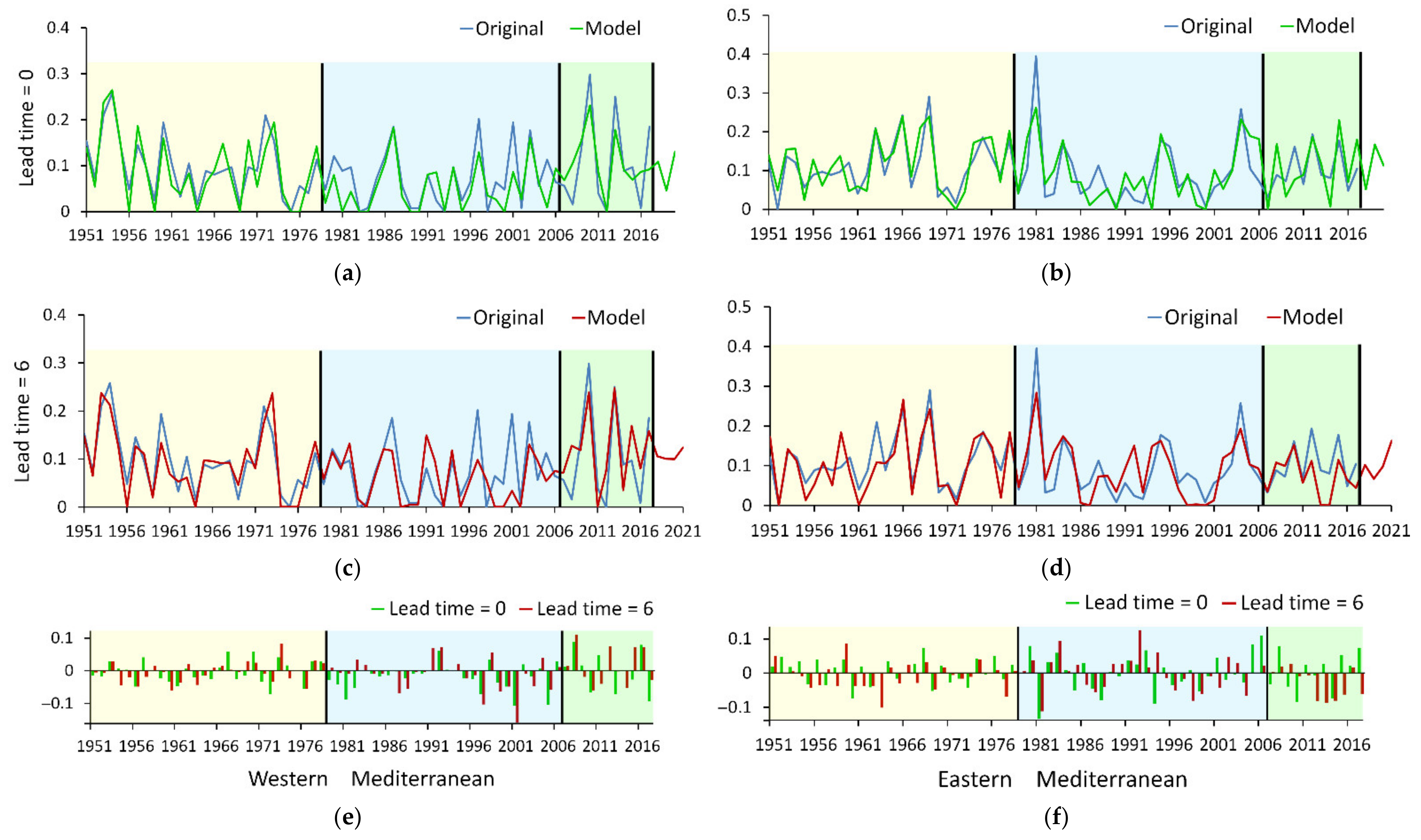
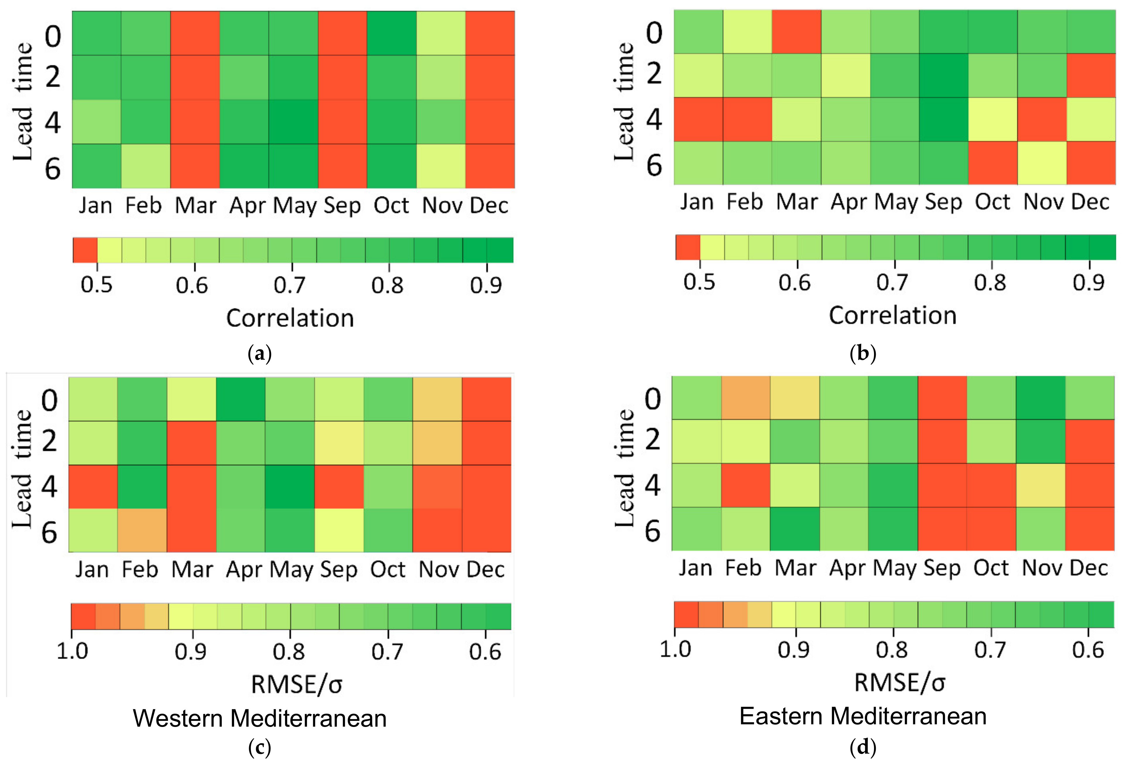
3.5. Neural Network Output

The results of the correlation analysis showed the absence of a single predictor for intense Mediterranean cyclones. The activity of intense cyclones each month and season was characterized by its own set of synchronous and asynchronous (leading) teleconnection signals and was the result of their interaction. This complicated the task of modeling intense cyclones taking into account the identified linear correlations with some atmospheric patterns. A solution for such a problem was a modeling based on the artificial neural network method, which allowed us to obtain the result of the nonlinear interaction of different predictors in the global ocean–atmosphere system. The indices of the teleconnection patterns were calculated using spatial correlation analysis between the high-frequency/low-frequency cyclone components and global fields of the 500 hPa geopotential height, wind components, and sea surface temperature (see Section 2.1 and Section 2.5).
The simulation was performed for intense cyclones of each month except summer months. Figure 11a–d shows a comparison of the model calculations and original (initial) values using the example of January for the two variations of the model: without the possibility of an advance forecast (synchronous model) and with the possibility of a forecast 6 months in advance (predictive model). Figure 11e,f shows that there was a comparable quality of modeling to the original series for both variations of the models.
For the Western Mediterranean (Figure 11a,c), the frequency of intense cyclones was reproduced well (r = 0.89) on the training sample. On the test period, the synchronous model was better (r = 0.77) than the predictive model (r = 0.61). However, on the control sample, both model variations managed to reproduce the initial frequency (r = 0.80–0.83).
For the Eastern Mediterranean (Figure 11b,d), on the training sample, the models described interannual variability in sufficient detail (r = 0.86). At the same time, January 1981 with the extremum of the frequency of intense cyclones occurred during the period outside the training sample. It should be expected that all subsequent similar extrema were underestimated by the model. On the test sample, the correlation coefficients for the two variations of the model were 0.76–0.77. On the control sample, the synchronous model showed a slightly better result (r = 0.70) than the model with the possibility of a 6-month advance forecast (r = 0.61).
Figure 12 shows the estimates of modeling of the frequency of intense cyclones in the Western and Eastern Mediterranean with a lead time of 0/2/4/6 months.
Modeling of the frequency of intense cyclones in the Western Mediterranean was successful for January, February, April, May, and October (Figure 12a,c) with a rather high quality of modeling. For example, the correlation coefficients in April, May, and October for a lead time of 6 months were in the range of 0.85–0.87, and the RMSE/σ ratio was 0.59–0.69. Modeling quality was low in November. According to the RMSE/σ ratio, the forecast in November was possible with a lead time up to 2 months.
Modeling of the frequency of intense cyclones in the Eastern Mediterranean was generally satisfactory in quality for each simulated month, except for December (Figure 12b,d). In October and November, the predictive capability of the model was limited to a lead time of up to 2 months. The highest correlation between the model calculations and the initial cyclone frequency was in September (r = 0.80–0.94), but the RMSE was greater than the standard deviation of the initial series (σ) due to the low frequency of intense cyclones. The best simulated month was May, for which the correlations for the different lead times were in the range of 0.70–0.78 and the RMSE/σ ratio was in the range of 0.57–0.67.

4. Discussion and Conclusions

Researchers usually study intense cyclones in the Mediterranean region in terms of physical and thermodynamic processes, e.g., [17], but not in terms of their temporal variability, which is better shown for the total frequency of cyclones, e.g., [18]. Understanding the variability patterns is important for long-term forecasts, especially regarding impactful intense cyclones.
In this paper, we studied the variability of time series of the frequency of intense and extreme cyclones in the Western and Eastern Mediterranean obtained using NCEP/NCAR reanalysis data [68] for the 1951–2017 period following the method of M.Y. Bardin [70,71]. The thresholds by intensity (average depth) were equal to the 75th percentile for intense cyclones and the 95th percentile for extreme cyclones (the variability of intense cyclones included the variability of extreme cyclones).
A comparison of the monthly, seasonal, and annual values of intense and extreme cyclones showed regional features for the Western and Eastern Mediterranean, which justified the approach of dividing the region into two parts when analyzing cyclonic activity, especially in autumn when there were significant differences (Figure 3). The annual frequencies of intense and extreme cyclones were higher in the Western Mediterranean, and the monthly values were higher in the Eastern Mediterranean in December–March for intense cyclones and January–March for extreme cyclones. At the same time, the summer season, due to the insignificant number of intense cyclones, was considered not to show any significant conclusions. For both regions of the Mediterranean, the greatest energy was concentrated in the winter spectra; the spring and autumn spectra were characterized by lower comparable magnitudes (Figure 7c–f).
As for tendencies, no significant linear trends were identified for intense and extreme cyclones in the Western Mediterranean. The only positive trend significant at the 90% confidence level was found for the autumn extreme cyclones over the Eastern Mediterranean (Figure 5c, Table 1) with a contribution to the variability of 5.2%. Due to this autumn trend, a positive annual trend was identified for extreme cyclones over the Eastern Mediterranean at the 85% confidence level (Figure 5d, Table 1), which was responsible for 3.6% of the variability. For intense cyclones over the Eastern Mediterranean, there was also a positive trend in autumn with a contribution to variability of 2.8% at the 80% confidence level (Figure 5b), and a negative trend in spring with a contribution of 3.2% at the 85% confidence level (Figure 5a).
According to previous studies, e.g., [6,9,86], significant linear trends were found in the total numbers of cyclones over the Mediterranean: a decrease over the Western Mediterranean and over the Black Sea, and an increase over the Eastern Mediterranean. According to our results, the trends of the numbers of intense and extreme cyclones in the Mediterranean region generally do not correspond to the trends of the total numbers of cyclones shown in [6,9,86]. The increase in autumn and decrease in spring only correspond to the results in [87] for the frequency of cyclones in the entire Mediterranean belt. At the same time, trends in different studies depend on the analyzed period, which complicates their comparison.
However, trends may indicate an anthropogenic signal in the climate series, which is caused by a linear increase in the concentration of carbon dioxide, and/or natural variability with periods comparable to the length of the series. On the one hand, significant linear trends in the Eastern Mediterranean, and insignificant in the Western Mediterranean, may correspond to the general pattern of an increase in regional temperature trends further to the continents (with an increase in the continentality of the regional climate). On the other hand, trends can be interpreted as part of the low-frequency variability, such as the Atlantic Multidecadal Oscillation and Pacific Decadal Oscillation. Then, there is correspondence with significant correlations of the frequency of intense cyclones with the AMO and PDO and the results of spectral analysis, which showed that the contribution of the decadal-multidecadal periodicities (≥10 years) almost reached 50% for intense cyclones over the Eastern Mediterranean in April. Stronger manifestations of the AMO and PDO periodicities in cyclones in the Eastern Mediterranean can be explained by the regional features of cyclone track schemes [52].
The results of the analysis of the variability of intense and extreme cyclones in the Mediterranean region are consistent with the results of our previous studies for the total numbers of cyclones in the Mediterranean-Black Sea region [88], as well for intense and extreme cyclones in the Black Sea region [10]. Temporal variability of intense cyclones in the Mediterranean region in 1951–2017 was characterized by background decadal fluctuations and prevailing interannual fluctuations with periods that were multiples of 2–3 years according to spectral analysis. In previous papers, we mentioned that such periods are typical for the main teleconnection patterns in the atmosphere (the North Atlantic Oscillation) and in the ocean (the El Niño–Southern Oscillation). In this study, we analyzed correlations with a wide range of teleconnection patterns in the ocean–atmosphere system and obtained both expected and original results.
For example, we expected that stronger synchronous correlations would be with the more regional climate patterns, such as the Mediterranean Oscillation. The results confirmed our expectations for the September–April period. However, for the Western Mediterranean Oscillation, no such stronger manifestations were found. It is understandable that the correlations with the East Atlantic Oscillation were stronger than with the North Atlantic Oscillation, because its high/low systems are closer to the region. According to [9], we expected a significant response to the Scandinavia pattern. Our results showed that its manifestations were at the level of the East Atlantic Oscillation but with the opposite sign (positive for the SCAND and negative for the EA). It is also reasonable that different teleconnection patterns made an additional contribution to the variability of intense cyclones in the Western and Eastern Mediterranean. An additional contribution was made in the Western Mediterranean by the patterns associated with the North Atlantic (AO, EA/WR), and in the Eastern Mediterranean by the patterns associated with Eurasia (POL/EUR).
Asynchronous responses in both groups of intense cyclones to the teleconnection indices were mainly with a delay of 1–3 and 5–8 months. For example, a delay ranging between 3 and 15 months was found between the onset of ENSO and its maximal impact on rainfall in Southern Europe [89]. La Niña manifestations in the Atlantic-European region were observed 1–2 months later after its mature stage, which is about 9 months after the onset [61]. In general, time lags may be associated with inter-basin teleconnection between the North Pacific and North Atlantic [53,90]. In our study, the Southern Oscillation manifested in an asynchronous correlation with a 7–8-month lag of cyclones in January (negative for WM intense cyclones) and November (negative for EM intense and extreme cyclones). However, there were also synchronous correlations with SOI in March (positive for WM intense cyclones and negative for EM extreme cyclones), April (positive for WM extreme cyclones), and spring (positive for WM intense cyclones). The North Pacific interannual patterns (PNA, EP/NP, and WP) correlated with both groups of intense Mediterranean cyclones, in some months synchronously and with lags of cyclones from 1 to 5 months. As for the manifestations of the multidecadal AMO and PDO patterns, the greatest responses (negative correlation) were found for cyclones in April, the time series of which were characterized by the greatest contribution of periodicities higher than 9 years (about 20%). Time lags of 2–9 months were common for the manifestations of AMO indices in April intense cyclones and PDO indices in April extreme cyclones. The results obtained may indicate that geographically remote teleconnection patterns can manifest through regional atmospheric centers of action, i.e., through regional teleconnection modes.
So, a variety of predictors that differ from month to month contribute to the temporal variability of intense cyclones in the Mediterranean region. In this regard, modeling cyclones requires a self-learning model with automatic selection of predictors. We used an artificial neural network model, which was suitable for this. The special algorithm selected atmospheric and oceanic indices corresponding to the atmospheric centers of action [25] and energy-active zones of the ocean [26]. This model was tested previously for intense cyclones in the Black Sea region [10] and showed good results. In this study, for the Western Mediterranean, quite a high-quality modeling was implemented for January, February, April, May, and October. For the Eastern Mediterranean, predictive capability for the frequency of intense cyclones was shown for each month from September to May, but it was limited to certain lead times for December, October, and November. In further studies, in order to avoid underestimation of extrema, the training sample should be extended to a period that includes the extreme values of the initial parameter. Anyway, the developed neural network model showed the potential to forecast the time evolution of the monthly frequency of cyclones and other climate variables with a lead time of 2 to 6 months using the monthly output of climate models.
In the short term, we suggest that a future research direction should be regional manifestations of cyclonic variability in the duration of the fire-hazardous period. In the long term, we are planning to focus on practical applications of our research findings for the assessment of the recreational capacity of resorts in the Mediterranean-Black Sea region.

Supplementary Materials

The following are available online at https://0-www-mdpi-com.brum.beds.ac.uk/article/10.3390/atmos12091218/s1. The monthly, seasonal and annual time series (1951–2017) of the frequency of total number/intense/extreme cyclones in the Western and Eastern Mediterranean.

Author Contributions

Conceptualization, V.N.M. and E.N.V.; methodology, V.N.M. and A.S.L.; software, A.S.L. and A.V.Y.; formal analysis, V.N.M. and A.S.L.; investigation, V.N.M. and A.S.L.; visualization, V.N.M., A.S.L. and A.V.Y.; writing—original draft, V.N.M. and A.S.L.; writing—review and editing, V.N.M. and E.N.V. All authors have read and agreed to the published version of the manuscript.

Funding

The reported study was funded by the state assignment of the Institute of Natural and Technical Systems within the research theme № 0012-2019-0007 and by RFBR and the Government of the Sevastopol according to the research project № 18-45-920068.

Institutional Review Board Statement

Not applicable.

Informed Consent Statement

Not applicable.

Data Availability Statement

The data presented in this study are available in Supplementary Materials.

Acknowledgments

The authors acknowledge Mikhail Bardin, Institute of Global Climate and Ecology, Institute of Geography of the Russian Academy of Sciences, Moscow, for his help with data and methodology. We acknowledge the free availability of data provided by the NOAA Climate Prediction Center, NOAA Physical Science Laboratory, and NCAR Climate Data Guide.

Conflicts of Interest

The authors declare no conflict of interest. The funders had no role in the design of the study; in the collection, analyses, or interpretation of data; in the writing of the manuscript, or in the decision to publish the results.

References

  1. Leckebusch, G.C.; Pinto, J.G. Extra-tropical cyclones in the present and future climate: A review. Appl. Clim. 2009, 96, 117–131. [Google Scholar] [CrossRef] [Green Version]
  2. Khromov, S.P.; Petrosyants, M.A. Meteorology and Climatology; MSU: Moscow, Russia, 2001; 528p. [Google Scholar]
  3. Trigo, I.F.; Bigg, G.R.; Davies, T.D. Climatology of cyclogenesis mechanisms in the Mediterranean. Mon. Weather Rev. 2002, 130, 549–569. [Google Scholar] [CrossRef]
  4. Alpert, P.; Neeman, B.U.; Shay-El, Y. Climatological analysis of Mediterranean cyclones using ECMWF data. Tellus A 1990, 42, 65–77. [Google Scholar] [CrossRef] [Green Version]
  5. Luterbacher, J.; Xoplaki, E.; Casty, C.; Wanner, H.; Pauling, A.; Küttel, M.; Rutishauser, T.; Brönnimann, S.; Fischer, E.; Fleitmann, D.; et al. Mediterranean climate variability over the last centuries: A review. Dev. Earth Environ. Sci. 2006, 4, 27–148. [Google Scholar] [CrossRef]
  6. Maheras, P.; Flocas, H.; Patrikas, I.; Anagnostopoulou, C. A 40 year objective climatology of surface cyclones in the Mediterranean region: Spatial and temporal distribution. Int. J. Clim. 2001, 21, 109–130. [Google Scholar] [CrossRef]
  7. Kouroutzoglou, J.; Flocas, H.A.; Keay, K.; Simmonds, I.; Hatzaki, M. Climatological aspects of explosive cyclones in the Mediterranean. Int. J. Clim. 2011, 31, 1785–1802. [Google Scholar] [CrossRef]
  8. Haylock, M.R.; Goodess, C.M. Interannual variability of European extreme winter rainfall and links with mean large-scale circulation. Int. J. Clim. 2004, 24, 759–776. [Google Scholar] [CrossRef]
  9. Nissen, K.M.; Leckebusch, G.C.; Pinto, J.G.; Renggli, D.; Ulbrich, S.; Ulbrich, U. Cyclones causing wind storms in the Mediterranean: Characteristics, trends and links to large-scale patterns. Nat. Hazards Earth Syst. Sci. 2010, 10, 1379–1391. [Google Scholar] [CrossRef]
  10. Maslova, V.N.; Voskresenskaya, E.N.; Lubkov, A.S.; Yurovsky, A.V.; Zhuravskiy, V.Y.; Evstigneev, V.P. Intense Cyclones in the Black Sea Region: Change, Variability, Predictability and Manifestations in the Storm Activity. Sustainability 2020, 12, 4468. [Google Scholar] [CrossRef]
  11. Jansa, A.; Genoves, A.; Garcia-Moya, J.A. Western Mediterranean cyclones and heavy rain. Part 1: Numerical experiment concerning the Piedmont flood case. Meteorol. Appl. 2000, 7, 323–333. [Google Scholar] [CrossRef]
  12. Zêzere, J.L.; Trigo, R.M.; Trigo, I.F. Shallow and deep landslides induced by rainfall in the Lisbon region (Portugal): Assessment of relationships with the North Atlantic Oscillation. Nat. Hazards Earth Syst. Sci. 2005, 5, 331–344. [Google Scholar] [CrossRef]
  13. Ziv, B.; Saaroni, H.; Yair, Y.; Ganot, M.; Baharad, A.; Isaschari, D. Atmospheric factors governing winter thunderstorms in the coastal region of the eastern Mediterranean. Appl. Clim. 2009, 95, 301–310. [Google Scholar] [CrossRef]
  14. Flaounas, E.; Kotroni, V.; Lagouvardos, K.; Kazadzis, S.; Gkikas, A.; Hatzianastassiou, N. Cyclone contribution to dust transport over the Mediterranean region. Atmos. Sci. Lett. 2015, 16, 473–478. [Google Scholar] [CrossRef] [Green Version]
  15. Bakkensen, L.A. Mediterranean hurricanes and associated damage estimates. J. Extrem. Events 2017, 4, 1750008. [Google Scholar] [CrossRef]
  16. Paliaga, G.; Faccini, F.; Luino, F.; Turconi, L.; Bobrowsky, P. Geomorphic processes and risk related to a large landslide dam in a highly urbanized Mediterranean catchment (Genova, Italy). Geomorphology 2019, 327, 48–61. [Google Scholar] [CrossRef]
  17. Flaounas, E.; Raveh-Rubin, S.; Wernli, H.; Drobinski, P.; Bastin, S. The dynamical structure of intense Mediterranean cyclones. Clim. Dyn. 2015, 44, 2411–2427. [Google Scholar] [CrossRef]
  18. Guijarro, J.A.; Jansa, A.; Campins, J. Time variability of cyclonic geostrophic circulation in the Mediterranean. Adv. Geosci. 2006, 7, 45–49. [Google Scholar] [CrossRef] [Green Version]
  19. Trigo, I.F.; Davies, T.D.; Bigg, G.R. Decline in Mediterranean rainfall caused by weakening of Mediterranean cyclones. Geophys. Res. Lett. 2000, 27, 2913–2916. [Google Scholar] [CrossRef]
  20. Campins, J.; Genovés, A.; Picornell, M.A.; Jansà, A. Climatology of Mediterranean cyclones using the ERA-40 dataset. Int. J. Clim. 2011, 31, 1596–1614. [Google Scholar] [CrossRef] [Green Version]
  21. Jansa, A.; Genoves, A.; Picornell, M.A.; Campins, J.; Radinovic, D.; Alpert, P. Mediterranean cyclones: Subject of a WMO project. Life Cycle Extratropical Cyclones 1994, 2, 26–31. [Google Scholar]
  22. Lionello, P.; Gacic, M.; Gomis, D.; Garcia-Herrera, R.; Giorgi, F.; Planton, S.; Trigo, R.; Theocharis, A.; Tsimplis, M.N.; Ulbrich, U.; et al. Program focuses on climate of the Mediterranean region. Eos Trans. Agu 2012, 93, 105–106. [Google Scholar] [CrossRef]
  23. Genovés, A.; Campins, J.; Jansà, A. Intense storms in the Mediterranean: A first description from the ERA-40 perspective. Adv. Geosci. 2006, 7, 163–168. [Google Scholar] [CrossRef] [Green Version]
  24. Jansa, A.; Alpert, P.; Arbogast, P.; Buzzi, A.; Ivancan-Picek, B.; Kotroni, V.; Llasat, M.C.; Ramis, C.; Richard, E.; Romero, R.; et al. MEDEX: A general overview. Nat. Hazards Earth Syst. Sci. 2014, 14, 1965–1984. [Google Scholar] [CrossRef] [Green Version]
  25. Sahsamanoglou, H.S. A contribution to the study of action centres in the North Atlantic. Int. J. Clim. 1990, 10, 247–261. [Google Scholar] [CrossRef]
  26. Kondrat’ev, K.I.; Kozoderov, V.V. Satellite observations of the earth’s radiation budget components and the problem of the energetically active zones of the world ocean (EAZO). In Vistas in Applied Mathematics: Numerical Analysis; Optimization Software, Inc.: New York, NY, USA, 1986; pp. 223–243. [Google Scholar]
  27. Barnston, A.G.; Livezey, R.E. Classification, seasonality and persistence of low-frequency atmospheric circulation patterns. Mon. Weather Rev. 1987, 115, 1083–1126. [Google Scholar] [CrossRef]
  28. Enfield, D.B.; Mestas-Nuñez, A.M. Multiscale variabilities in global sea surface temperatures and their relationships with tropospheric climate patterns. J. Clim. 1999, 12, 2719–2733. [Google Scholar] [CrossRef]
  29. Van Loon, H.; Rogers, J.C. The seesaw in winter temperatures between Greenland and northern Europe. Part I: General description. Mon. Weather Rev. 1978, 106, 296–310. [Google Scholar] [CrossRef] [Green Version]
  30. Rogers, J.C.; Van Loon, H. The seesaw in winter temperatures between Greenland and northern Europe. Part II: Some oceanic and atmospheric effects in middle and high latitudes. Mon. Weather Rev. 1979, 107, 509–519. [Google Scholar] [CrossRef]
  31. Rogers, J.C. Patterns of low-frequency monthly sea level pressure variability (1899–1986) and associated wave cyclone frequencies. J. Clim. 1990, 3, 1364–1379. [Google Scholar] [CrossRef] [Green Version]
  32. Trenberth, K.E.; Hurrell, J.W. Decadal atmosphere-ocean variations in the Pacific. Clim. Dyn. 1994, 9, 303–319. [Google Scholar] [CrossRef]
  33. Hurrell, J.W. Transient eddy forcing of the rotational flow during northern winter. J. Atmos. Sci. 1995, 52, 2286–2301. [Google Scholar] [CrossRef] [Green Version]
  34. Hurrell, J.W. Decadal trends in the North Atlantic Oscillation: Regional temperatures and precipitation. Science 1995, 269, 676–679. [Google Scholar] [CrossRef] [PubMed] [Green Version]
  35. Schlesinger, M.E.; Ramankutty, N. An oscillation in the global climate system of period 65–70 years. Nature 1994, 367, 723–726. [Google Scholar] [CrossRef]
  36. Knight, J.R.; Folland, C.K.; Scaife, A.A. Climate impacts of the Atlantic Multidecadal Oscillation. Geophys. Res. Lett. 2006, 33, L17706. [Google Scholar] [CrossRef] [Green Version]
  37. Zhang, Y.; Wallace, J.M.; Battisti, D.S. ENSO-like interdecadal variability: 1900–93. J. Clim. 1997, 10, 1004–1020. [Google Scholar] [CrossRef]
  38. Mantua, N.J.; Hare, S.R.; Zhang, Y.; Wallace, J.M.; Francis, R.C. A Pacific interdecadal climate oscillation with impacts on salmon production. Bull. Am. Meteorol. Soc. 1997, 78, 1069–1079. [Google Scholar] [CrossRef]
  39. Trenberth, K.E.; Caron, J.M. The Southern Oscillation Revisited: Sea Level Pressures, Surface Temperatures, and Precipitation. J. Clim. 2000, 13, 4358–4365. [Google Scholar] [CrossRef]
  40. Wallace, J.M.; Gutzler, D.S. Teleconnections in the geopotential height field during the northern hemisphere winter. Mon. Weather Rev. 1981, 109, 784–812. [Google Scholar] [CrossRef]
  41. Voskresenskaya, E.N.; Polonsky, A.B. Air pressure fluctuations in the North Atlantic and their relationship with El Nino-southern oscillations. Phys. Oceanogr. 1993, 4, 275–282. [Google Scholar] [CrossRef]
  42. Serreze, M.C.; Carse, F.; Barry, R.G.; Rogers, J.C. Icelandic low cyclone activity: Climatological features, linkages with the NAO, and relationships with recent changes in the Northern Hemisphere circulation. J. Clim. 1997, 10, 453–464. [Google Scholar] [CrossRef]
  43. Hurrell, J.W.; Deser, C. North Atlantic climate variability: The role of the North Atlantic Oscillation. J. Mar. Syst. 2010, 79, 231–244. [Google Scholar] [CrossRef]
  44. Moore, G.W.K.; Renfrew, I.A. Cold European winters: Interplay between the NAO and the East Atlantic mode. Atmos. Sci. Lett. 2012, 13, 1–8. [Google Scholar] [CrossRef]
  45. Nesterov, E.S. East Atlantic oscillation of the atmospheric circulation. Russ. Meteorol. Hydrol. 2009, 34, 794–800. [Google Scholar] [CrossRef]
  46. Gao, N.; Bueh, C.; Xie, Z.; Gong, Y. A novel identification of the Polar/Eurasia pattern and its weather impact in May. J. Meteorol. Res. 2019, 33, 810–825. [Google Scholar] [CrossRef]
  47. Kaznacheeva, V.D.; Shuvalov, S.V. Climatic characteristics of Mediterranean cyclones. Russ. Meteorol. Hydrol. 2012, 37, 315–323. [Google Scholar] [CrossRef]
  48. Mändla, K.; Jaagus, J.; Sepp, M. Climatology of cyclones with southern origin in northern Europe during 1948–2010. Appl. Clim. 2015, 120, 75–86. [Google Scholar] [CrossRef]
  49. Romanski, J.; Romanou, A.; Bauer, M.; Tselioudis, G. Teleconnections, midlatitude cyclones and Aegean Sea turbulent heat flux variability on daily through decadal time scales. Reg. Environ. Chang. 2014, 14, 1713–1723. [Google Scholar] [CrossRef] [Green Version]
  50. Cassou, C.; Terray, L. Dual influence of Atlantic and Pacific SST anomalies on the North Atlantic/Europe winter climate. Geophys. Res. Lett. 2001, 28, 3195–3198. [Google Scholar] [CrossRef] [Green Version]
  51. Bardin, M.Y.; Voskresenskaya, E.N. Pacific decadal oscillation and European climatic anomalies. Phys. Oceanogr. 2007, 17, 200–208. [Google Scholar] [CrossRef]
  52. Voskresenskaya, E.; Maslova, V. Joint manifestations of PDO (Pacific Decadal Oscillation) and negative AMO (Atlantic Multidecadal Oscillation) phases in winter cyclonic activity. J. Environ. Sci. Eng. A 2012, 1, 1325. [Google Scholar]
  53. Drouard, M.; Rivière, G.; Arbogast, P. The link between the North Pacific climate variability and the North Atlantic Oscillation via downstream propagation of synoptic waves. J. Clim. 2015, 28, 3957–3976. [Google Scholar] [CrossRef]
  54. Alpert, P.; Baldi, M.; Ilani, R.; Krichak, S.; Price, C.; Rodo, X.; Saaroni, H.; Ziv, B.; Kishcha, P.; Barkan, J.; et al. Relations between climate variability in the Mediterranean region and the tropics: ENSO, South Asian and African monsoons, hurricanes and Saharan dust. In Developments in Earth and Environmental Sciences; Lionello, P., Malanotte-Rizzoli, P., Boscolo, R., Eds.; Elsevier: Amsterdam, The Netherlands, 2006; Volume 4, pp. 149–177. [Google Scholar] [CrossRef]
  55. Brönnimann, S.; Xoplaki, E.; Casty, C.; Pauling, A.; Luterbacher, J.J.C.D. ENSO influence on Europe during the last centuries. Clim. Dyn. 2007, 28, 181–197. [Google Scholar] [CrossRef] [Green Version]
  56. Kamil, S.; Almazroui, M.; Kucharski, F.; Kang, I.S. Multidecadal changes in the relationship of storm frequency over Euro-Mediterranean region and ENSO during boreal winter. Earth Syst. Environ. 2017, 1, 1–10. [Google Scholar] [CrossRef]
  57. Hardiman, S.C.; Dunstone, N.J.; Scaife, A.A.; Smith, D.M.; Knight, J.R.; Davies, P.; Claus, M.; Greatbatch, R.J. Predictability of European winter 2019/20: Indian Ocean dipole impacts on the NAO. Atmos. Sci. Lett. 2000, 21, e1005. [Google Scholar] [CrossRef]
  58. Polonsky, A.B.; Basharin, D.V. How strong is the impact of the Indo-ocean dipole on the surface air temperature/sea level pressure anomalies in the Mediterranean region? Glob. Planet. Chang. 2017, 151, 101–107. [Google Scholar] [CrossRef]
  59. Graf, H.F.; Zanchettin, D. Central Pacific El Niño, the “subtropical bridge,” and Eurasian climate. J. Geophys. Res. Atmos. 2012, 117. [Google Scholar] [CrossRef] [Green Version]
  60. Ding, S.; Chen, W.; Feng, J.; Graf, H.F. Combined impacts of PDO and two types of La Niña on climate anomalies in Europe. J. Clim. 2017, 30, 3253–3278. [Google Scholar] [CrossRef]
  61. Voskresenskaya, E.N.; Marchukova, O.V.; Maslova, V.N.; Lubkov, A.S. Interannual climate anomalies in the Atlantic-European region associated with La-Nina types. In IOP Conference Series: Earth and Environmental Science; IOP Publishing: Bristol, UK, 2018; Volume 107, p. 012043. [Google Scholar] [CrossRef]
  62. Picornell, M.A.; Jansa, A.; Genovés, A.; Campins, J. Automated database of mesocyclones from the HIRLAM (INM)-0.5° analyses in the western Mediterranean. Int. J. Clim. 2001, 21, 335–354. [Google Scholar] [CrossRef]
  63. Conte, M.; Giuffrida, A.; Tedesco, S. The Mediterranean oscillation: Impact on precipitation and hydrology in Italy. In Proceedings of the Conference on Climate and Water, Helsinki, Finland, 11–15 September 1989; Publications of Academy of Finland: Helsinki, Finland, 1989; Volume 1, pp. 121–137. [Google Scholar]
  64. Dünkeloh, A.; Jacobeit, J. Circulation dynamics of Mediterranean precipitation variability 1948–98. Int. J. Clim. 2003, 23, 1843–1866. [Google Scholar] [CrossRef]
  65. Maheras, P.; Xoplaki, E.; Kutiel, H. Wet and dry monthly anomalies across the Mediterranean basin and their relationship with correlation, 1860–1990. Appl. Clim. 1999, 64, 189–199. [Google Scholar] [CrossRef]
  66. Martin-Vide, J.; Lopez-Bustins, J.A. The western Mediterranean oscillation and rainfall in the Iberian Peninsula. Int. J. Clim. J. R. Meteorol. Soc. 2006, 26, 1455–1475. [Google Scholar] [CrossRef]
  67. Lubkov, A.S.; Voskresenskaya, E.N.; Marchukova, O.V. Forecasting El Niño/La Niña and Their Types Using Neural Networks. Russ. Meteorol. Hydrol. 2020, 45, 806–813. [Google Scholar] [CrossRef]
  68. Kalnay, E.; Kanamitsu, M.; Kistler, R.; Collins, W.; Deaven, D.; Gandin, L.; Iredell, M.; Saha, S.; White, G.; Woollen, J.; et al. The NCEP/NCAR 40-year reanalysis project. Bull. Am. Meteorol. Soc. 1996, 77, 437–471. [Google Scholar] [CrossRef] [Green Version]
  69. Rayner, N.A.; Parker, D.E.; Horton, E.B.; Folland, C.K.; Alexander, L.V.; Rowell, D.P.; Kent, E.C.; Kaplan, A. Global analyses of sea surface temperature, sea ice, and night marine air temperature since the late nineteenth century. J. Geophys. Res. 2003, 108, 4407. [Google Scholar] [CrossRef]
  70. Bardin, M.Y. Variability of cyclonicity characteristics in the middle troposphere of temperate latitudes of the Northern Hemisphere. Russ. Meteorol. Hydrol. 1995, 11, 24–37. [Google Scholar]
  71. Bardin, M.Y.; Polonsky, A.B. North Atlantic oscillation and synoptic variability in the European-Atlantic region in winter. Izv. Atmos. Ocean. Phys. 2005, 41, 127–136. [Google Scholar]
  72. Neu, U.; Akperov, M.G.; Bellenbaum, N.; Benestad, R.S.; Blender, R.; Caballero, R.; Cocozza, A.; Dacre, H.F.; Feng, Y.; Fraedrich, K.; et al. IMILAST: A Community Effort to Intercompare Extratropical Cyclone Detection and Tracking Algorithms. Bull. Am. Meteorol. Soc. 2013, 94, 529–547. [Google Scholar] [CrossRef]
  73. Gil, V.E.; Genovés, A.; Picornell, M.A.; Jansa, A. Automated database of cyclones from the ECMWF model: Preliminary comparison between west and east Mediterranean basins. In Proceedings of the 4th EGS Plinius Conference, Mallorca, Spain, 2–4 October 2002. [Google Scholar]
  74. Alexandersson, H.; Tuomenvirta, H.; Schmith, T.; Iden, K. Trends of storms in NW Europe derived from an updated pressure data set. Clim. Res. 2000, 14, 71–73. [Google Scholar] [CrossRef] [Green Version]
  75. Matulla, C.; Schoner, W.; Alexandersson, H.; von Storch, H.; Wang, X.L. European storminess: Late nineteenth century to present. Clim. Dyn. 2008, 31, 125–130. [Google Scholar] [CrossRef]
  76. Parzen, E. On estimation of a probability density function and mode. Ann. Math. Stat. 1962, 33, 1065–1076. [Google Scholar] [CrossRef]
  77. Duin, R.P.W. On the Choice of Smoothing Parameters for Parzen Estimators of Probability Density Functions. IEEE Trans. Comput. 1976, 25, 1175–1179. [Google Scholar] [CrossRef]
  78. Lubkov, A.; Voskresenskaya, E.; Kukushkin, A. Method for reconstructing the monthly mean water transparencies for the northwestern part of the Black Sea as an example. Atmos. Ocean. Opt. 2016, 29, 457–464. [Google Scholar] [CrossRef]
  79. Osovsky, S. Neural Networks for Data Processing; Finansy i Statistika: Moscow, Russia, 2004; p. 344. [Google Scholar]
  80. Haykin, S. Neural Networks: A Comprehensive Foundation; Prentice Hall PTR: Upper Saddle River, NJ, USA, 1994. [Google Scholar]
  81. Stocker, T. (Ed.) Climate Change 2013: The Physical Science Basis: Working Group I Contribution to the Fifth Assessment Report of the Intergovernmental Panel on Climate Change; Cambridge University Press: Cambridge, MA, USA, 2014. [Google Scholar]
  82. Polonsky, A. The Ocean’s Role in Climate Change; Cambridge Scholars Publishing: Newcastle upon Tyne, UK, 2019; 276p. [Google Scholar]
  83. Gamiz-Fortis, S.R.; Pozo-Vazquez, D.; Esteban-Parra, M.J.; Castro-Diez, Y. Spectral characteristics and predictability of the NAO assessed through Singular Spectral Analysis. J. Geophys. Res. Atmos. 2002, 107, 15. [Google Scholar] [CrossRef]
  84. Seip, K.L.; Gron, O. On the statistical nature of distinct cycles in global warming variables. Clim. Dyn. 2019, 52, 7329–7337. [Google Scholar] [CrossRef]
  85. Kinter, J.L.; Miyakoda, K.; Yang, S. Recent change in the connection from the Asian monsoon to ENSO. J. Clim. 2002, 15, 1203–1215. [Google Scholar] [CrossRef]
  86. Trigo, I.F. Climatology and interannual variability of storm-tracks in the Euro-Atlantic sector: A comparison between ERA-40 and NCEP/NCAR reanalyses. Clim. Dynam. 2005, 26, 127–143. [Google Scholar] [CrossRef]
  87. Bartholy, J.; Pongrácz, R.; Pattantyús-Ábrahám, M. Analyzing the genesis, intensity, and tracks of western Mediterranean cyclones. Appl. Clim. 2009, 96, 133–144. [Google Scholar] [CrossRef]
  88. Maslova, V.; Voskresenskaya, E.; Bardin, M. Variability of the cyclone activity in the Mediterranean-Black Sea region. J. Environ. Prot. Ecol. 2010, 11, 1366–1372. [Google Scholar]
  89. Rodó, X.; Baert, E.; Comin, F.A. Variations in seasonal rainfall in Southern Europe during the present century: Relationships with the North Atlantic Oscillation and the El Niño-Southern Oscillation. Clim. Dyn. 1997, 13, 275–284. [Google Scholar] [CrossRef]
  90. Gong, Z.; Sun, C.; Li, J.; Feng, J.; Xie, F.; Ding, R.; Yang, Y.; Xue, J. An inter-basin teleconnection from the North Atlantic to the subarctic North Pacific at multidecadal time scales. Clim. Dyn. 2020, 54, 807–822. [Google Scholar] [CrossRef]
Figure 1. The total number of the centers of all identified local minima for the 1951–2017 period on a 6-h basis (red shading) and the boundaries of the Western and Eastern Mediterranean (blue boxes).
Atmosphere 12 01218 g001
Figure 2. Frequency of intense cyclones in January (both y-axes) in the Western Mediterranean: the original series (blue line), high-frequency (green line), and low-frequency (red line) components.
Atmosphere 12 01218 g002
Figure 3. Seasonal/annual (a,b) and monthly (c,d) averages of the frequency of intense/extreme cyclones over the Western and Eastern Mediterranean (WMC-75/WMC-95 and EMC-75/EMC-95, respectively): (a,c) intense cyclones; (b,d) extreme cyclones. Error bars correspond to the 95% confidence level.
Atmosphere 12 01218 g003
Figure 4. Time plots of the frequency of total number/intense/extreme cyclones over the Western and Eastern Mediterranean (WMC/WMC-75/WMC-95 and EMC/EMC-75/EMC-95, respectively): (a,b) winter averages; (c,d) annual averages.
Atmosphere 12 01218 g004
Figure 5. Time plots and linear trends (straight black lines) of standardized anomalies of the frequency of intense/extreme cyclones over the Eastern Mediterranean (EMC-75/EMC-95): (a) spring intense cyclones; (b) autumn intense cyclones; (c) autumn extreme cyclones; (d) annual extreme cyclones.
Atmosphere 12 01218 g005
Figure 6. Correlations of the 1000 hPa geopotential height with global temperature for the (a) annual series, (b) winter series, (c) spring series, and (d) autumn series. Correlation coefficients r < −0.2 and r > +0.2 are significant at the 90% confidence level.
Atmosphere 12 01218 g006aAtmosphere 12 01218 g006b
Figure 7. Averaged periodograms of annual (a,b) and seasonal (cf) values of the frequency of intense/extreme cyclones over the Western and Eastern Mediterranean (WMC-75/WMC-95 and EMC-75/EMC-95, respectively): (a,c,e) intense cyclones; (b,d,f) extreme cyclones.
Atmosphere 12 01218 g007aAtmosphere 12 01218 g007b
Figure 8. April correlations of the 1000 hPa geopotential height with the (a) AMO and (b) PDO indices. Correlation coefficients r < −0.2 and r > +0.2 are significant at the 90% confidence level.
Atmosphere 12 01218 g008
Figure 9. Winter correlations of the 1000 hPa geopotential height with the (a) NAO and (b) AO indices. Correlation coefficients r < −0.2 and r > +0.2 are significant at the 90% confidence level.
Atmosphere 12 01218 g009
Figure 10. Winter correlations of the 1000 hPa geopotential height with the (a) EA/WR and (b) TNH indices. Correlation coefficients r<−0.2 and r > + 0.2 are significant at the 90% confidence level.
Atmosphere 12 01218 g010
Figure 11. The frequency of intense cyclones in January: initial values (original) and model simulations (model) over the Western (a,c) and Eastern (b,d) Mediterranean for the two variations of the model: without the possibility of an advance forecast (lead time = 0) (a,b) and with the possibility of a forecast 6 months in advance (lead time = 6) (c,d). Vertical black lines mark the range of the training sample (1951–1978), test sample (1979–2006), control sample (2007–2017), and modeling period without the initial values of cyclones (2018–2021). Below, there are absolute error diagrams of the synchronous model (green bars) and the model with a lead time of 6 months (red bars) for the Western (e) and Eastern (f) Mediterranean.
Atmosphere 12 01218 g011
Figure 12. The diagrams of correlation (a,b) and RMSE/σ (c,d) for lead times of 0, 2, 4, and 6 months between the modeled and original frequency of intense cyclones in the Western (a,c) and Eastern (b,d) Mediterranean. Correlation coefficient significant at α = 0.01 (for the number of degrees of freedom n = 11) is 0.49.
Atmosphere 12 01218 g012
Table 1. Characteristics of linear trends of the frequency of intense/extreme cyclones over the Western and Eastern Mediterranean (WMC-75/WMC-95 and EMC-75/EMC-95, respectively): coefficient of the trend equation (klin), level of significance (p-probability = 100/(p-value)), coefficient of determination (rlin2). Significant values are highlighted in bold.
Frequency Parameterklin,
×10−3
p-Probability, %r2lin,
%
WMC-75
winter−5.3860.21.1
spring−4.1448.40.7
autumn6.0665.91.4
annual−4.4951.80.8
WMC-95
winter−1.9924.50.2
spring3.4040.60.4
autumn0.040.50.0
annual−1.8823.10.1
EMC-75
winter0.060.80.0
spring−9.1885.33.2
autumn8.6282.62.8
annual−2.1326.20.2
EMC-95
winter6.3067.81.5
spring7.8878.52.4
autumn11.6893.65.2
annual9.7487.63.6
Table 2. Periods (years) of spectral peaks (significant at the 75% confidence level) contributing at least 8% to the dispersion of the seasonal (except summer) and annual frequency of intense/extreme cyclones over the Western and Eastern Mediterranean (WMC-75/WMC-95 and EMC-75/EMC-95, respectively).
Averaging TimeWMC-75WMC-95EMC-75EMC-95
winter2,4; 8.32.4; 4.72.3; 3.33.9; 7.3
spring2.22.2; 7.32.2 2.1; 3.9
autumn2.92.1; 4.42.22.1; 3.3
annual3.9; 8.32.63.52.4; 8.3
Publisher’s Note: MDPI stays neutral with regard to jurisdictional claims in published maps and institutional affiliations.

