Chemical Composition and Source Apportionment of Total Suspended Particulate in the Central Himalayan Region

Abstract

The present study analyzes data from total suspended particulate (TSP) samples collected during 3 years (2005–2008) at Nainital, central Himalayas, India and analyzed for carbonaceous aerosols (organic carbon (OC) and elemental carbon (EC)) and inorganic species, focusing on the assessment of primary and secondary organic carbon contributions (POC, SOC, respectively) and on source apportionment by positive matrix factorization (PMF). An average TSP concentration of 69.6 ± 51.8 µg m⁻³ was found, exhibiting a pre-monsoon (March–May) maximum (92.9 ± 48.5 µg m⁻³) due to dust transport and forest fires and a monsoon (June–August) minimum due to atmospheric washout, while carbonaceous aerosols and inorganic species expressed a similar seasonality. The mean OC/EC ratio (8.0 ± 3.3) and the good correlations between OC, EC, and nss-K⁺ suggested that biomass burning (BB) was one of the major contributing factors to aerosols in Nainital. Using the EC tracer method, along with several approaches for the determination of the (OC/EC)pri ratio, the estimated SOC component accounted for ~25% (19.3–29.7%). Furthermore, TSP source apportionment via PMF allowed for a better understanding of the aerosol sources in the Central Himalayan region. The key aerosol sources over Nainital were BB (27%), secondary sulfate (20%), secondary nitrate (9%), mineral dust (34%), and long-range transported mixed marine aerosol (10%). The potential source contribution function (PSCF) and concentration weighted trajectory (CWT) analyses were also used to identify the probable regional source areas of resolved aerosol sources. The main source regions for aerosols in Nainital were the plains in northwest India and Pakistan, polluted cities like Delhi, the Thar Desert, and the Arabian Sea area. The outcomes of the present study are expected to elucidate the atmospheric chemistry, emission source origins, and transport pathways of aerosols over the central Himalayan region.

1. Introduction

Deterioration of air quality is a global concern, particularly in South and Southeast Asia, where levels of pollutants frequently exceed the air quality guidelines established by WHO and the National Pollution Control Board of India [1,2,3]. Particulate matter (PM) pollution originates from both natural and anthropogenic sources and has major impacts, not only on air quality and human health, but also on the Earth’s radiation budget, visibility, and cloud formation [4,5]. In India, several studies have examined the chemical composition of particulate matter (i.e., total suspended particulates, TSP; PM₁₀, PM_2.5) and observed high contributions of carbonaceous aerosols (EC, OC) in fractions of 30–35% for TSP over the Indo-Gangetic Plain (IGP) region [6,7,8,9]. The concentrations and composition of airborne particles depend on their sources and atmospheric processes, as well as on the meteorological conditions [10,11]. Therefore, the identification and quantitative characterization of contributing sources and atmospheric processes for aerosol formation are very important to link the emissions with observed levels and develop air pollution control strategies [12,13,14].

The fundamental principle of receptor models (RMs) is the mass conservation between the source and the receptor site [15]. The chemical mass balance (CMB) models require detailed prior knowledge of sources and emission inventories. For the second major category of receptor models, information on chemical components that are related to specific sources at the receptor site is used for source apportionment. Several approaches for the second RM type exist, such as positive matrix factorization (PMF), UNMIX, principal component analysis/absolute principal component scores (PCA/APCS), etc. [16,17,18,19,20,21]. Over South Asia, PMF and PCA techniques have been frequently used for apportioning sources of size-segregated aerosols (PM_2.5, PM_10, or TSP), with approximately 70% of the total source apportionment studies having been performed using PMF, PCA, or related factor analytic techniques [13].

The vast majority of studies dealing with carbonaceous aerosols, chemical composition, and radiative effects of black carbon (BC) and brown carbon (BrC) in India have been performed over the IGP region (e.g., Delhi [22,23,24], Agra [25], Patiala [10,26], Kanpur [5,27], and Varanasi [28,29]). These studies have enhanced the current knowledge on the chemical composition, sources, seasonality, mixing processes, and radiative impacts of size-segregated aerosols. The main sources of carbonaceous aerosols over the IGP are mainly fossil fuel combustion, biomass/wood burning, traffic/industrial emissions, as well as agricultural waste burning emissions. These aerosols can be uplifted by prevailing winds up to the central Himalayan region, or even in the Tibetan Plateau, and significantly affect the Himalayan climate and glaciology [30].

The Himalayan region, with a unique role in the Asian climate, is considered as a vulnerable environment regarding aerosol dynamics and impacts. Several chemical speciation studies have been performed for carbonaceous aerosols and inorganic species over the western and central Himalayan regions during the last decade, reporting the dominance of transported aerosol plumes from the IGP [7,31,32,33,34,35,36]. However, there is a knowledge gap regarding the primary and secondary organic carbon (POC, SOC) fractions [7], along with a lack of receptor modeling works in the central Indian Himalayas. Furthermore, source apportionment studies over the central Himalayan region are required for assessment of contributions and temporal variability of sources that influence the area through regional transport.

Ram et al. [7] characterized the aerosol levels, chemical composition, and optical properties in the central Himalayan region, using TSP samples collected at the high-altitude site of Nainital (February 2005 to February 2008), and focusing on the long-term trends and seasonality. The current study uses this chemical speciation dataset to estimate the POC and SOC components via the EC tracer method, using various approaches for the determination of the primary OC/EC ratio. This work also performs a first-time source apportionment analysis using this dataset, focusing on the seasonality of sources and regional transport over the central Himalayan area. Source apportionment was performed using the PMF receptor model, along with potential source contribution function (PSCF) and concentration weighted trajectory (CWT) analyses, aiming to associate each factor with specific source regions. This is the first receptor modeling study in the central Himalayan region and can provide reference information on local/distant aerosol source contributions and supplement emission inventories, with the overarching goal of supporting the assessment of climate impacts over the central Himalayan region.

2. Study Area and Measurements

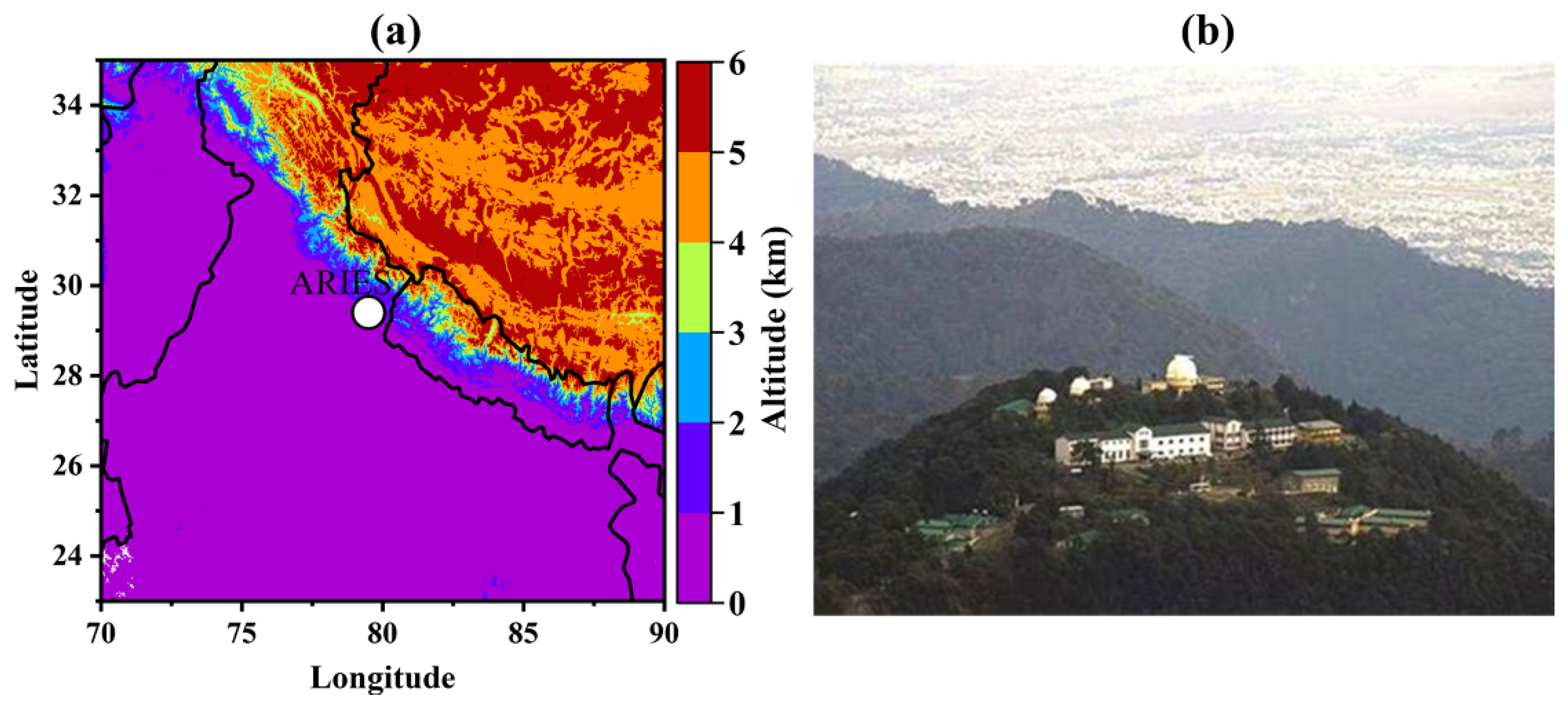
2.1. Site Description

The observational site Manora Peak hill (29.39° N, 79.45° E, 1958 m a.s.l.), Nainital, is a high-altitude site in the Gangetic Himalayan (GH) region that is surrounded by forested areas and high-altitude mountains to the northeast and opens to the Ganges valley to the southwest (Figure 1). The site is far away from large-scale industries, power plants, and major polluted cities (about 235 km away from Delhi) [34,37]. The site is located in a sparsely populated area with a total population of 0.5 million (according to the 2011 census) and is considered representative for background and regional conditions and strategically located for climate change studies [38]. Smoke plumes from paddy and wheat residue burning affect the site in post-monsoon/autumn period (September–November) and in pre-monsoon/spring (March–April), respectively [39,40], while, in winter, carbonaceous aerosols from local wood-burning emissions for domestic heating are enhanced [34,41]. During the summer/monsoon months (June–August), the long-range transported dust dominates due to the escalation of dust activity over the Thar Desert and Southwest Asia [42]. The geographical and atmospheric conditions in Nainital efficiently represent the background conditions in the central Indian Himalayas, while polluted air masses from the Ganges valley affect the site, being strongly dependent on prevailing meteorology and boundary-layer dynamics [43,44,45].

2.2. Aerosol Sampling and Chemical Analysis

This study is based on results of chemical analysis in TSP samples that were previously collected onto pre-combusted quartz-fiber filters (PALLFLEX^TM, 2500QAT-UP; size: 20.0 × 25.4 cm²) using an Andersen’s high-volume sampler (Envirotech APM-430; Envirotech Instruments Pvt. Ltd., New Delhi, India, http://www.envirotechindia.com, accessed on 15 September 2021), operating at an average flow rate of 1 m³ min⁻¹. The sampling duration ranged between 15 and 20 h, while the sampling frequency was initially fixed to one sample per two weeks, and later increased to one sample per week. In total, this study utilized 65 samples that were collected during the period February 2005 to February 2008, and chemically analyzed as described elsewhere [7,46]. The TSP and chemical analysis dataset that is used here for source apportionment was initially presented by Ram et al. [7] and extended up to July 2008. However, from March 2008 to July 2008, water-soluble organic carbon (WSOC) and cation samples were not determined. Therefore, for the sake of consistency in the dataset, results from March 2008 to July 2008 were not considered and 65 samples (February 2005–February 2008) were used for further analysis.

The quartz filters were analyzed for OC and EC mass concentrations using a Sunset Carbon analyzer (Sunset Laboratory; https://www.sunlab.com/, accessed on 15 September 2021) following the NIOSH-5040 (National Institute of Occupational Safety and Health) protocol [7,47,48]. For the determination of WSOC and water-soluble inorganic species (WSIS) concentrations, one fourth of the filter (approximately 105 cm²) was immersed in 50 mL of ultrapure water (resistivity: 18.2 MΩ) and ultrasonicated for 6–8 h. Using the water extracts, WSOC was measured using a total organic carbon (TOC) analyzer (Shimadzu model TOC 5000A) and WSIS (Na⁺, K⁺, NH₄⁺, Mg²⁺, Ca²⁺, Cl⁻, NO₃⁻, and SO₄²⁻) were analyzed by ion chromatography (Dionex; Model DX-500). Details about the chemical analysis, including sample preparation, protocols, and quality assurance, are discussed elsewhere [7,46,48].

3. Methodology

3.1. Estimation of POC and SOC

In the current study, the POC and SOC mass concentrations were estimated via the EC tracer method [49,50]. This method is based on measured OC and EC mass concentrations and the use of an appropriate primary OC-to-EC ratio:

$$\mathrm{POC}=\left[\mathrm{EC}\right]\times {\left(\frac{\mathrm{OC}}{\mathrm{EC}}\right)}_{\mathrm{Pri}}$$

(1)

$$\mathrm{SOC}=\left[\mathrm{OC}\right]-\left[\mathrm{POC}\right]=\left[\mathrm{OC}\right]-\left[\mathrm{EC}\right]\times {\left(\frac{\mathrm{OC}}{\mathrm{EC}}\right)}_{\mathrm{Pri}}$$

(2)

where the (OC/EC)_pri is the primary OC/EC ratio in freshly emitted combustion aerosols. The critical point of the EC tracer method is to determine a representative value of the (OC/EC)_pri ratio, which is site-, source-, and aerosol-type-specific and highly sensitive to the method used for its determination [49,51]. There are several approaches reported in the literature for the estimation of (OC/EC)_pri, such as consideration of the minimum OC/EC ratio, estimation using the lower percentiles (e.g., 5–25%) of OC/EC, the minimum R-square (MRS) method, as well as different regression techniques [51,52,53]. Recently, Wu et al. (2019) [51] combined the EC tracer method with MRS and found more robust estimates of SOC compared to those based on (OC/EC)_min and lower OC/EC percentiles. The main assumption of the MRS method is that the EC is inherently unrelated to SOC and, hence, the (OC/EC)_pri should be the ratio resulting in minimum correlation (near-zero R²) between estimated SOC and measured EC [51,53]. In this study, the POC and SOC components were estimated in Nainital from the 65 samples using three approaches, i.e., (OC/OC)_min, 25% OC/EC percentile, and MRS, allowing the stability of the estimated SOC fractions to be examined.

3.2. Ion Balance and Neutralization Factors

An ion balance check was performed using the assumption that the anions (Cl⁻, NO₃⁻, and SO₄²⁻) and cations (Na⁺, NH₄⁺, K⁺, Mg²⁺, and Ca²⁺) make up the majority of water-soluble ions. According to the charge conservation law, the total cation equivalents (CE) and total anion equivalents (AE) must be equal. The AE (CE) is estimated as a sum of each anion (cation) divided by its equivalent weight. The percent ion difference (ID [%]) was estimated from the following equation:

$$\mathrm{ID}[\%]=\parallel \frac{\mathrm{CE}-\mathrm{AE}}{\mathrm{CE}+\mathrm{AE}}\parallel \times 100$$

(3)

Neutralization factor (NF) calculations for the individual cations were used to measure their acid neutralization potential. Previous studies assumed that Na⁺ and Cl⁻ entirely originate from sea salt and, therefore, omitted their contribution to NF calculations [54]. However, the present site, which is far from the sea, is unlikely to receive fresh marine contributions. Furthermore, a very poor correlation (R² = 0.05; Figure 2) between Na⁺ and Cl⁻, along with a significantly lower (0.07) ratio of Cl⁻/Na⁺ compared to seawater (1.8), justify the low impact of marine sources over the measurement site [55,56]. However, the Himalayan region may have a small amount of NaCl embedded in the soil in the form of halite, which may be detected in the air due to natural resuspension processes [57]. In the present study, the Na⁺ concentrations (0.52 µg m⁻³) were much higher than that of Cl⁻ (0.04 µg m⁻³), suggesting depletion of Cl⁻, as HNO₃ reacts with NaCl to form HCl [58]. Therefore, the influence of Na⁺ ions in the neutralization process was assessed using non-sea salt [Na⁺]. The non-sea salt [Na⁺] can be estimated by subtracting 0.56× [Cl⁻] from [Na⁺]. The NFs were then calculated as:

$$\mathrm{NF}\left({\mathrm{Na}}^{+}\right)=\left(\left[{\mathrm{Na}}^{+}\right]-0.56\left[{\mathrm{Cl}}^{-}\right]\right)/\left(2\left[{\mathrm{SO}}_4^{2-}\right]+\left[{\mathrm{NO}}_3^{-}\right]\right)$$

(4)

$$\mathrm{NF}\left({\mathrm{K}}^{+}\right)=\left[{\mathrm{K}}^{+}\right]/\left(2\left[{\mathrm{SO}}_4^{2-}\right]+\left[{\mathrm{NO}}_3^{-}\right]\right)$$

(5)

$$\mathrm{NF}\left({\mathrm{Ca}}^{2+}\right)=\left[{\mathrm{Ca}}^{2+}\right]/\left(\left[{\mathrm{SO}}_4^{2-}\right]+2\left[{\mathrm{NO}}_3^{-}\right]\right)$$

(6)

$$\mathrm{NF}\left({\mathrm{Mg}}^{2+}\right)=\left[{\mathrm{Mg}}^{2+}\right]/\left(\left[{\mathrm{SO}}_4^{2-}\right]+2\left[{\mathrm{NO}}_3^{-}\right]\right)$$

(7)

$$\mathrm{NF}\left({\mathrm{NH}}_4^{+}\right)=\left[{\mathrm{NH}}_4^{+}\right]/\left(2\left[{\mathrm{SO}}_4^{2-}\right]+\left[{\mathrm{NO}}_3^{-}\right]\right)$$

(8)

3.3. Source Apportionment via PMF Receptor Model

The positive matrix factorization (PMF) is a multivariate receptor model [15] that has been widely used for PM source apportionment in India [2,4,22,59]. The chemical mass balance equation can be written as:

$$X_{ij}={\displaystyle \sum }_{k=1}^p{g}_{ik}{f}_{kj}+e_{ij}$$

(9)

where X and e are the measured concentration and the residual matrixes of dimensions i (sample number) and j (chemical species), while g and f are source profile and source contribution matrixes, respectively, with k = 1… p (p being the total number of sources).

In this study, using the EPA PMF 5.0 software [60], models were run with 65 samples, each one with data for 11 chemical species. Based on the number of model variables, the number of samples here is considered adequate to perform PMF analysis, according to the rules of thumb established by guidance documents [61] and as displayed by several previously published studies (e.g., [15,18,19,20,59]). Missing values were replaced with the geometric mean concentration of corresponding species. The uncertainty (σ_ij) input file was generated using the detection limit of each species and the concentration in each sample [62,63]. Low-uncertainty (strong) species were classified based on S/N (signal/noise) ratios greater than 2, whereas species with an S/N ratio between 0.2 and 2.0 were labeled as weak and their uncertainties were increased three times [64]. The S/N ratios for each species included in the PMF analysis were greater than 2, except Cl⁻ (S/N = 1.21). Since WSOC is a part of OC, it was also down-weighted by categorizing it as weak in order to limit double counting. Further details of the PMF process and the equations used in uncertainty analysis are provided in the Supplementary Materials (S.1.1), while the error indices are included in Table S1. For solutions with 2 to 8 factors, the Q_robust/Q_exp. ratio, the maximum individual mean of scaled residual (ISM), and maximum individual standard deviation of scaled residual (ISR) were calculated to gain insights in the optimum number of sources (see Figure S1). The ratio of Q_robust/Q_exp. values showed a drastic decrease for 3- to 5-factor solutions. The ISM and ISR also showed a sharp decline up to factor 5 and, beyond that, a steady change was observed in ISM and ISR. Therefore, the solutions of 4-, 5-, and 6-factor sources (Figure S1) were examined to identify the most physically interpretable solution. The scatter plots between the measured and modeled TSP revealed that the best fit was achieved by the 5-factor model, as compared to the 4- and 6-factor solutions (Figure S2). This solution was also characterized by a limited fraction of unexplained TSP mass (3.27%). The coefficient of determination (R²) between measured and modeled concentrations of each species, except Cl⁻ (R² = 0.2), was greater than 0.8 for the 5-factor solution. In addition, the PMF BS, DISP, and BS–DISP error estimates were more stable in the 5-factor solution (Table S1). A comparison of emission sources identified by the PMF simulation for factors four, five, and six is shown in the Supplementary Materials (Figures S3–S5). Regarding the 4-factor PMF solution, it could not separate the BB and secondary sources, while, in the 6-factor solution, there was a splitting of the soil dust source. Therefore, the 5-factor solution was selected and further analyzed, with results presented in Section 4.4.

3.4. Air Mass Back-Trajectory and Probability Functions (PSCF and CWT) Analysis

To track the source areas and transport pathways of the chemical species and identified factors over the study site, we performed air mass back-trajectory analysis using the hybrid single-particle Lagrangian integrated (HYSPLIT) model ([65,66], READY: http://www.ready.noaa.gov, accessed on 24 June 2021). In this work, five days’ (120 h) air mass back-trajectories were calculated at 14:00 h (local time) at 500 m above ground level.

The potential source contribution function (PSCF) and concentration weighted trajectory (CWT) are trajectory ensemble models developed to identify the transport pathways and potential source regions of pollutants affecting receptor sites [37,67]. The PSCF is the conditional probability that an air parcel arriving at the receptor site, and passed over an area traversed by the identified back-trajectories, had a pollutant concentration exceeding a predefined threshold. Therefore, the PSCF value for a grid cell i, j is described as:

$${\mathrm{PSCF}}_{ij}=\frac{m_{ij }}{n_{ij}}$$

(10)

where n_ij represents the total number of times the trajectories passed through the grid cell (i, j) and m_ij represents the total number of high source-related concentration events when the trajectories passed over the cell (i, j). The number of m_ij events was determined based on the 90th percentile of source contributions. To reduce the impact of cells with few data, a weighting factor was applied [67,68]. The probability for each cell (i, j) was multiplied by weighting functions W(ij):

$$W{\left(n\right)}_{ij}=\{\begin{array}{c}\begin{array}{c}1.00, n_{ij}>2\overline{n}\\ 0.75, \overline{n}< n_{ij} \le 2 \overline{n}\\ 0.50, \frac{\overline{n}}{2}<\overline{n_{ij}} \le \overline{n}\\ 0.15, n_{ij}\le \frac{\overline{n}}{2}\end{array} \end{array}$$

(11)

where, $\overline{n}$ is the average number of endpoints per cell, computed for every cell with at least one endpoint. The main drawback of the PSCF method is that several grid cells may have the same PSCF value if the sample concentrations are marginally higher or much higher than the required percentile criteria, so it could be difficult to differentiate between sources of modest and strong impact. Therefore, the CWT approach is widely used to tackle this issue [28,37,69]. The CWT field for a grid cell i, j (C_ij) is calculated as:

$$C_{ij}=\frac{1}{{{\displaystyle \sum }}_{m=1}^N{\tau }_{ijm}} {\displaystyle \sum }_{m=1}^N{C}_{m }{\tau }_{ijm}$$

(12)

where C_m is the estimated source contribution at the study location for trajectory m, and τ_ijm is the residence time of trajectory m in grid cell (𝑖, 𝑗), while N is the total number of trajectories. In this study, the PSCF and CWT analyses were used to identify the geographic areas that are associated with increased net contributions of the PMF-identified sources. The PSCF and CWT maps (and also the map in Figure 1 and the correlogram in Figure 2) were produced using the R-4.1.0 software, while the rest of the figures were plotted using the Origin 2021 suite.

4. Results and Discussion

4.1. TSP Mass and Chemical Composition

This section presents the TSP, carbonaceous aerosol and inorganic species concentrations, and seasonality for the 65 analyzed samples. Since detailed analysis of the concentrations and seasonality was given in Ram et al. [7], even with slightly different results due to the higher number of samples and small differences in the delineation of seasons, only a brief description is given here for the essential knowledge about aerosol chemical composition in Nainital. A descriptive summary of concentrations of measured chemical species in TSP is listed in

Table 1. The arithmetic mean (AM), standard deviation (SD), range (minimum and maximum) of concentrations, and method detection limits (MDL) for TSP, OC, EC, WSOC, and WSIS. The number of samples with chemical species below detection limits and the number of missing values are also included.

Species	AM (µg m−3)	SD (µg m−3)	Min (µg m−3)	Max (µg m−3)	MDL (µg m−3)	No. of BDL Values	No. of Missing Values
TSP	69.58	51.79	12.67	271.69	--	--	--
OC	8.62	5.14	1.31	22.28	0.80	0	0
EC	1.19	0.78	0.14	3.07	0.15	1	0
WSOC	4.91	3.17	0.89	15.42	0.05	0	1
TC (OC + EC)	9.81	5.86	1.45	24.52	--	--	--
Cl−	0.04	0.07	0.00	0.45	0.01	16	1
NO3−	0.57	0.73	0.00	3.18	0.03‘	5	4
SO42−	4.68	3.20	0.79	16.04	0.03	0	1
Na+	0.52	0.45	0.04	1.41	0.02	0	1
NH4+	0.61	0.73	0.01	3.65	0.02	5	3
K+	0.46	0.37	0.02	1.77	0.02	1	1
Mg2+	0.15	0.08	0.02	0.34	0.02	0	1
Ca2+	1.40	0.99	0.14	4.65	0.03	0	1
Total Ions	8.24	5.14	0.93	26.98	--	--	--

, while the seasonal mean concentrations are listed in Table S2. TSP concentrations in Nainital ranged from 12.7 to 271.7 µg m⁻³, with an average of 69.6 ± 51.8 µg m⁻³. The average concentration of total carbon (OC + EC) was 9.8 ± 5.9 µg m⁻³, accounting for 14% of the TSP mass.

On a seasonal basis, the maximum TSP (86.3 ± 45.4 µg m⁻³) and carbonaceous aerosol (OC, EC) concentrations were observed in spring (March–May), with medium to high TSP levels in the post-monsoon period (September–November) and winter (December–February) (59.9 ± 31.4 µg m⁻³ and 64.4 ± 43.9 µg m⁻³, respectively). TSP, OC, and EC concentrations were lower during the summer monsoon (June–August) (64.8 ± 73.4, 4.4 ± 2.4, and 0.5 ± 0.2 µg m⁻³) as a result of aerosol wet removal over the measurement site, and the IGP as well [7]. The seasonal variation of EC and OC, which is slightly different than that presented in Ram et al. [7], shows an agreement with previous studies over Darjeeling in the eastern Himalayas [33,70] and Srinagar in Garhwal Himalayas [71]. Moderate to high levels of OC, EC, and K⁺ in October–November and March–April, as well as high correlations (r > 0.83) between them (Figure 2), indicate a strong influence from agricultural waste burning following the harvesting periods of rice and wheat, respectively, in Punjab and Haryana states in the northwest IGP [34,37,72]. The highest concentrations of EC and OC (Table S2) in winter could be attributed to the lower boundary layer height, along with wood and waste material burning for domestic heating. The average WSIS concentration was 8.24 ± 5.14 µg m⁻³, which corresponds to about 12% of the TSP mass, and was much lower than the levels reported over IGP sites [29,54,59,73]. Nitrates maximized—rather unexpectedly—in the pre-monsoon period (0.84 μg m⁻³), while sulfates did so in post-monsoon (6.25 μg m⁻³), and K⁺ also in post-monsoon (Table S2), due to the important influence from paddy residue burning in northwest IGP [72].

Figure 2 presents the Pearson correlation coefficients among the concentrations of TSP constituents. The high correlation between OC and EC (r = 0.91) indicates the common presence of combustion sources. The OC/EC ratio is widely used for characterizing the pollution sources and separating between primary and secondary emissions [74]. In this study, the OC/EC ratio ranged widely from 4.8 to 27.2, with an average of 8.0 ± 3.3, indicating a relatively high fraction of organic aerosols from biomass burning and/or enhanced contribution from SOC formation [48,75]. The non-sea-salt potassium (nss-K⁺ = K⁺ − 0.037 × Na⁺) that is considered as a tracer for BB aerosols had an average concentration of 0.45 ± 0.36 μg m⁻³ (~93% of total K⁺), indicating low contributions from marine sources [26,40]. The ratios nss-K⁺/EC and nss-K⁺/OC have been used for the apportionment of BB sources [7,73]. The nss-K⁺ was highly correlated (r = 0.82–0.85) with OC and EC, while the nss-K⁺/EC ratio was found to be 0.35 ± 0.16 (range of 0.08–0.85) [7], lower than that (0.51 ± 0.41; 0.63–0.69) found in Patiala, northwest IGP, during peak agricultural burning periods [10]. The 95th percentile nss-K⁺/EC value of 0.66 can be considered as characteristic for BB emissions in Nainital, being close to the upper limit of 1.1 proposed by Andreae and Merlet (2001) for (nss-K⁺/EC)_bb [76]. On the other hand, the nss-K⁺/OC ratio ranged from 0.02 to 0.09 (mean of 0.05 ± 0.02), generally within the range reported for BB aerosols (0.04 to 0.13) [26,76].

On the other hand, the WSOC/OC ratio provides information of aerosol hygroscopicity, emission sources, and aging processes in the atmosphere [77,78,79]. The WSOC/OC ratio ranged from 0.33 to 0.93 (average of 0.57 ± 0.15), with high variability between the samples, but without a distinct seasonal pattern [7]. An average value of 0.60 ± 0.20 was reported for the WSOC/OC ratio over a higher altitude site in the western Himalayas (Himansh observatory; 32.4° N, 77.6° E, 4080 m) [80]. These high ratios suggest the dominance of aged aerosols over the central Himalayas, associated with transported carbonaceous aerosols from the IGP [34,75].

4.2. Ion Chemistry and Neutralization Factor

The total CE and AE values were calculated at 9.41 and 6.84, respectively, with a total percent ion difference of 14.22% and a good correlation of R² = 0.73 (Figure S6). The anion deficit showed significant correlation (R² = 0.59) with Ca²⁺, indicating an alkaline environment over the site, likely attributed to carbonate species (CO₃²⁻) in dust particles that were sampled but not quantified by IC [57,81].

The calculated NF values followed the order of Ca²⁺ = 0.26, Na⁺ = 0.07, K⁺ = 0.05, NH₄⁺ = 0.05, and Mg²⁺ = 0.03, indicating that Ca²⁺ was the leading neutralizing acid for TSP in Nainital. However, the NF results indicated that the overall cation concentration was insufficient to completely neutralize the charge of sulfate and nitrate ions. Moreover, the zero correlation between the NH₄⁺ and NO₃⁻ suggests that NH₄NO₃ formation is of minor importance (see Figure 2). The NF (NH₄⁺) (Equation (8)) suggested that sulfate and nitrate have a very small chance of being totally or partially neutralized. This finding suggests the presence of sulfuric acid (H₂SO₄) and ammonium bisulfate ((NH₄)HSO₄), along with ammonium sulfate ((NH₄)₂SO₄) in Nainital (7).

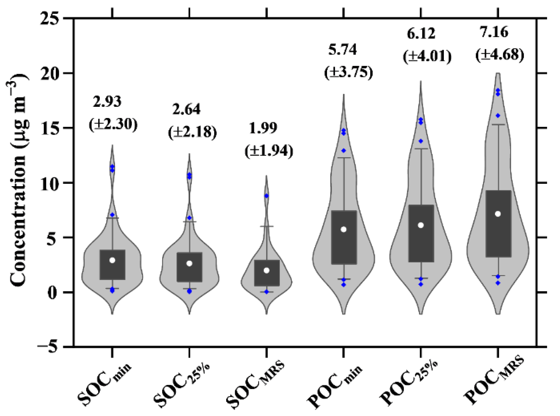
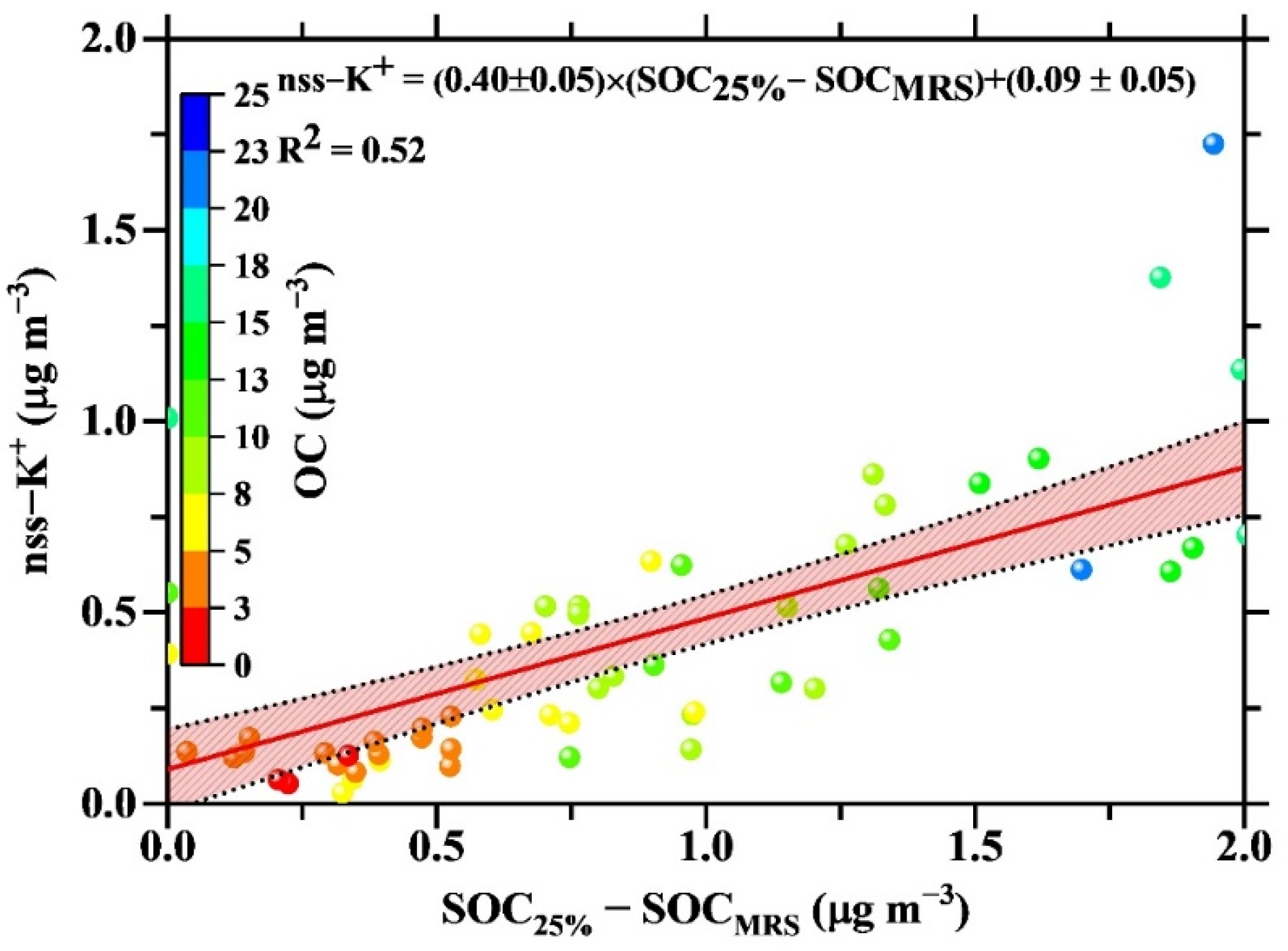
4.3. Estimates of POC and SOC

In this study, the SOC and POC were estimated using the EC tracer method, but with different techniques for the determination of the (OC/EC)_pri, allowing the robustness of the SOC and POC estimations to be examined. The (OC/EC)_min value was 4.81 and was initially used as the primary ratio for estimations of POC and SOC via Equations (1) and (2). In addition, data corresponding to the lowest 25% of OC/EC ratios were also considered for the primary OC/EC ratio and, via linear regressions of OC vs. EC, an (OC/EC)_pri ratio of 5.13 was estimated. On the other hand, the MRS method [51,82] estimated a slightly higher (OC/EC)_pri ratio of 6.0. These varying (OC/EC)_pri ratios indicate the uncertainty in the quantification of POC and SOC components with the EC tracer method, which increases significantly in environments highly affected by BB aerosols [53]. The POC and SOC components estimated by different (OC/EC)_pri ratios in Nainital are shown in Figure 3.

The SOC estimated via the MRS method exhibited an average concentration of 1.99 ± 1.94 μg m⁻³, which corresponds to 23% of the total OC mass. The SOC concentrations estimated using the minimum OC/EC ratio and 25th percentile showed slightly higher concentrations of 2.93 ± 2.30 μg m⁻³ and 2.64 ± 2.18 μg m⁻³, respectively, corresponding to 34% and 31%, respectively, of the total OC mass concentration. Consequently, POC components dominated in all estimations, exhibiting fractions of 66–71% (Figure 3). It is characteristic that all approaches resulted in similar distributions of the POC and SOC concentrations (Figure 3). The percentage contributions of POC, SOC, and EC to total carbon (TC = EC + OC) mass at Nainital are summarized in

Table 2. Percentage contributions of POC, SOC (estimated via EC tracer, percentile, and MRS methods), and EC to total carbon (TC = OC + EC) mass at Nainital for the entire study period and for four different seasons.

Methods	Annual			Winter			Spring			Summer			Autumn
	EC (%)	POC (%)	SOC (%)	EC (%)	POC (%)	SOC (%)	EC (%)	POC (%)	SOC (%)	EC (%)	POC (%)	SOC (%)	EC (%)	POC (%)	SOC (%)
EC tracer	12.1	58.2	29.7	13.0	62.3	24.7	12.4	59.7	27.9	9.8	47.2	43.0	11.7	56.1	32.2
25%	12.0	61.5	26.5	12.8	65.7	21.5	12.1	62.1	25.8	9.8	50.4	39.8	11.7	59.8	28.5
MRS	11.5	69.2	19.3	11.9	71.6	16.5	12.0	71.9	16.1	9.3	55.7	35.0	11.5	69.0	19.5

. On an annual basis, the POC component prevailed, with fractions ranging from 58.2% to 69.2%, while the SOC fraction was much lower (19.3% to 29.7%) and the EC fraction was 11.5–12.1% (Table 2). The POC fraction increases in winter and spring seasons and is lowest in summer, when secondary aerosol formation is favored due to the intense photochemical processes and enhanced presence of volatile organic compounds (VOCs) and oxidizing agents, such as O₃ and OH radicals [7,75]. Furthermore, the higher temperatures during spring and summer facilitate primary biogenic emissions [46]. The increased POC fraction in winter indicates the effect of local combustion emissions and an enhanced contribution from wood burning for domestic heating in local and neighboring areas, as well as transported plumes from the plains [34,37,44,48].

The highest POC concentrations combined with a strong correlation between OC and nss-K⁺ in winter justify POC formation from primary emissions of biomass burning. This is supported by the strong correlations (R² = 0.68) between POC and nss-K⁺, independently of the approach used for POC estimation (Figure 4). The small differences between the POC and SOC concentrations from the various approaches indicate a consistency in the estimations and reliable results for Nainital. The differences in SOC estimates between the 25th percentile and MRS methods were significantly related with nss-K⁺ (R² = 0.52; Figure 5). This might be related to fast oxidation processes of BB aerosols, which are considered as secondary in the 25% approach but as primary in the MRS approach due to their significant association with EC emissions from biomass burning [51,53].

The WSOC/OC ratio has been extensively used to assess secondary organic aerosol (SOA) formation, since SOA mostly contains photochemically produced polar functional groups, which are soluble in water [83,84]. However, WSOC may also have sources from primary BB aerosols, as many studies in IGP have shown [10,13,27]. Therefore, a good correlation between WSOC and estimated SOC can help justify the current SOC estimates. Here, the analysis showed a regression R² of 0.35 (slope = 0.43 ± 0.81) between WSOC and SOC estimates using the (OC/EC)_min, while similar results were found for the other two approaches. The SOC concentration was much lower (2.93 ± 2.30 μg m⁻³ for (OC/EC)_min) than that of WSOC (4.91 ± 3.17 μg m⁻³), most likely corresponding to the soluble nature of BB aerosols transported from the IGP [10,11,40], which have been classified as POC in the current estimates.

Previous studies in north India reported that estimated SOC contributed 43–49% to the total PM_2.5 OC in urban Delhi [85] and accounted for 18%, 25%, and 60% of OC at traffic, rural, and remote sites, respectively, in Agra [86]. At Gual Pahari, a rural site close to New Delhi, the SOC fraction to total OC was 46% for PM_2.5 samples [9]. Another study in Delhi [50] showed a 50% contribution of SOC on an annual basis, with an increased SOC formation in summer monsoon and winter periods, which was attributed to fast oxidation processes under a highly turbid environment during wintertime, when fog processing highly affected SOC formation [11]. Regarding the application of the EC tracer method in TSP samples, annual average SOC fractions in the range of 39% to 51% were estimated in Agra, India for samples highly affected by BB during post-monsoon and winter periods [87]. SOC fractions of 27%, 49%, 41%, and 35% to the OC mass were estimated during pre-monsoon, monsoon, post-monsoon, and winter periods, respectively, in Darjeeling, eastern Himalayas [70].

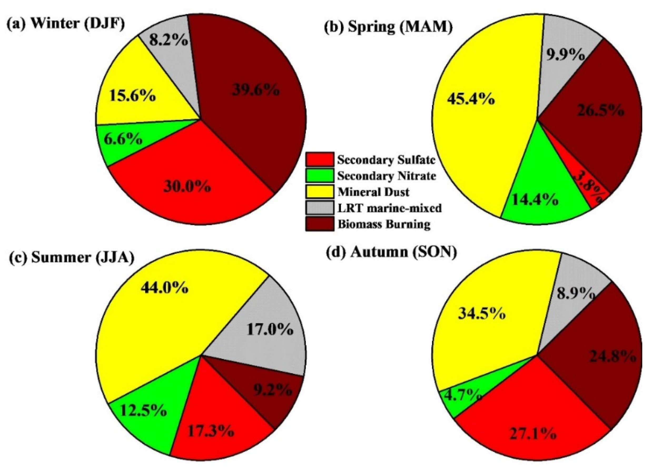
4.4. Source Identification via PMF Receptor Model

The PMF receptor model was applied to determine the sources of aerosols over Nainital, based on the 5-factor solution, as described in Section 3.3 and in the Supplementary Materials. The 5-factor solution is presented in Figure 6, while Figure 7 displays the percentage (%) contribution of each PMF-identified source to the reconstructed mass on a seasonal basis. As mentioned previously, only a small percent of TSP mass (3.27%) was left unexplained by the PMF model.

Factor 1 (secondary sulfate): The first factor was identified as secondary sulfate (SS_f) and contributed 19.8% to TSP mass (Figure 6), with a remarkable seasonal variability, from 3.8% in spring/pre-monsoon to 30% in winter (Figure 7). This factor accounted for approximately 90% of the variation in NH₄⁺ and 49% in SO₄²⁻, indicating secondary atmospheric processes for fine aerosol formation [7,22]. Large quantities of SO₂ are emitted by the combustion of sulfur-rich fuels, such as coal and crude oil from power plants in the NW IGP [28]. PSCF and CWT analyses have identified potential source origins for Factor 1 in Pakistan and N-NW Indian states (Figure 8 and Figure S7). However, the PSCF analysis also indicated distant sources in Iran, the Persian Gulf, and the Caspian Sea regions, areas with intense oil production and refining activities that comprise a significant source of precursor SO_x emissions [88]. In Punjab and Haryana states of NW India, agricultural fertilizer use and animal husbandry are important sources of gaseous ammonia emissions, which are significant over continental sites where acid is neutralized by ammonia and mineral dust, leading to secondary aerosol formation [59].

Factor 2 (secondary nitrate/inorganic aerosol): This factor was mostly characterized by secondary nitrate and non-sea-salt chloride (nss-Cl⁻), and contributed 9.1% to TSP mass (Figure 6), explaining about 86% of the variance in NO₃⁻ and 43% in Cl⁻. Since Na⁺ was not included in the factor profile along with chloride, it was assumed that the chloride was nss-Cl⁻. Cl⁻ concentrations were very low (0.04 μg m⁻³) and originated from waste burning (see also its significant fraction in Factor 5; Figure 6) and/or aged sea salt. Higher contributions were observed for Ca²⁺ and Mg²⁺ with respect to ammonium, as soil particles bound acidic gases in the coarse mode [89]. This factor exhibited the highest contribution to TSP mass in spring (14%) and summer (13%), despite unfavorable warm conditions for partitioning of nitrate and chloride in the particle phase (Figure 7). This indicates a substantial intensification of precursor emissions and their transport to the receptor site during the warm period. PMF did not distinguish between nitrate and nss-Cl⁻, possibly due to a common origin of secondary inorganic aerosol precursors, such as coal combustion and small- to medium-scale refining industries in Haryana, Punjab, and Pakistan to the northwest of Nainital, affecting the receptor site when northwesterlies prevail [37,50]. The PSCF and CWT analyses (Figure 8 and Figure S7) revealed North and East Pakistan, Jammu and Kashmir, Punjab, and Haryana states in NW India as potential source areas for this factor. Enhanced HCl emissions from coal combustion in power plants have been previously recorded over NW IGP [90].

Factor 3 (mineral dust): The third factor represents the soil dust source and contributed 33.5% to TSP mass. This factor was dominated by Ca²⁺ (46% explained variance) and registered significant contributions to Mg²⁺ (28%) and SO₄²⁻ (33%) (Figure 6). The coexistence of Ca²⁺ with SO₄²⁻ in this factor underlines the formation of calcium sulfate (CaSO₄) in the coarse particle fraction. The highest contributions of this factor to TSP were observed, as expected, in spring (45%) and summer (44%) (Figure 7), in agreement with the highest dust activity in the Thar Desert and Southwest Asia [42], while the lowest fraction was recorded in winter (15.6%). The PSCF analysis (Figure 8) suggested that the major source locations for this factor are in north Pakistan, the Thar Desert, and desert areas in East Africa, which are important source regions of mineral dust. The well-defined southwest monsoon air flow over the Arabian Sea that carries dust-laden air masses over the Himalayan range is also notable (Figure 8).

Factor 4 (long-range transport marine mixed): This factor addressed about 80% of the variation in Na⁺ and contributed 10.2% to TSP mass. This factor contains moderate amounts of nitrate and sulfate that could be identified as aged sea spray from long-range transport, where Cl⁻ has been depleted over the Indian mainland. The PSCF plot shows a potential origin from the Arabian Sea and indicates possible mixing with dust during the passage of the air masses over the Thar Desert and arid regions in Pakistan (Figure 8) [9]. In general, the influence of marine air masses and such aerosol types at Nainital and the western Himalayas is expected to be very weak [34,45] and, indeed, the factor recorded low contributions to TSP (8–10%), except for summer (17%), when advection of marine aerosols by strong SW winds is favored in the setting of the summer monsoon [91].

Factor 5 (biomass burning): The fifth factor is related to processed BB aerosols and is identified by the high contributions to OC, EC, WSOC, combined with K⁺, which is a good BB tracer at sites not directly affected by marine aerosol intrusions [10]. The factor explained approximately 58%, 59%, 57%, and 55% of the variance in OC, EC, WSOC, and K⁺, respectively (Figure 6). Cl⁻ also received a significant contribution from the biomass burning source (~32%), although its mass concentration was generally low. Several studies in India have verified the affinity of chloride with biomass burning sources [92,93]. The high OC/EC ratio of 6.9 in the source profile is indicative of processed BB emissions. This factor was most dominant during winter (39.6%) due to biomass/wood burning for heating in the IGP and the Himalayas [35], but it also exhibited high contributions in spring and autumn seasons (27% and 25% of TSP) due to agricultural crop residue burning in NW IGP (Figure 7). The contribution of this factor was minimized in summer (9%), as a result of reduced primary BB emissions and the prevalence of effective atmospheric cleaning mechanisms. The PSCF and CWT analyses indicated major BB source areas in Himachal Pradesh and Uttarakhand due to springtime forest fires in the Himalayas [39,94,95] and also in Punjab (Figure 8), where extensive agricultural BB takes place in post-monsoon (paddy residue burning) and pre-monsoon (wheat residue burning) seasons [40,96,97].

5. Summary and Conclusions

In this study, we examined the chemical composition of total suspended particulate (TSP) samples collected in Nainital, a high-altitude site in the central Himalayan region, for a period of three years, from February 2005 to February 2008. Since TSP concentrations, chemical composition, and seasonality have been the subject of previous works, the current analysis focused mainly on TSP source apportionment using receptor modeling (PMF) and the estimation of secondary organic carbon (SOC), using various approaches in the EC tracer method. The TSP mass concentration in Nainital ranged from 12.7 to 271.7 µg m⁻³, with an average value of 69.6 ± 51.8 µg m⁻³. The highest TSP concentrations were observed in spring due to enhanced dust transport and forest fires over the surrounding regions, while, during the summer monsoon, TSP, OC, and EC levels minimized due to wet removal.

Carbonaceous aerosols (OC, EC) maximized in winter due to the intensification of biomass burning (e.g., wood burning, crop residual burning, etc.) over the IGP and the Himalayas for domestic heating and the shallower mixing layer. The high OC/EC ratio (8.0 ± 3.3), along with a good correlation between OC, EC, and nss-K⁺, suggested a significant effect of biomass-burning aerosols, while the relatively high WSOC/OC ratio (0.57 ± 0.15) indicated significant contributions of biomass burning, secondary, or aged organic aerosols over Nainital. The estimated SOC fractions via the EC tracer method accounted for ~25% (ranges of 19.3–29.7%) of total carbon (OC + EC), and were consistent between different approaches for the calculation of primary OC/EC ratios in the EC tracer method.

The PMF source apportionment results revealed that the main aerosol sources (factors) in Nainital were mineral dust (34%), biomass burning (27%), secondary sulfate (20%), secondary nitrate (9%), and long-range transported marine mixed aerosols (10%), which exhibited a distinct seasonality as well, with predominance of mineral dust in spring and summer, and biomass burning and secondary sulfate in winter. The source area identification, based on the potential source contribution function (PSCF) and concentration weighted trajectory (CWT) methods, showed that TSP was mainly transported from Punjab and Haryana states in NW India and northeast Pakistan, while the Thar Desert and East Africa significantly contributed to the presence of dust-related aerosols over the central Himalayas. The transported marine mixed aerosol source was mainly associated with SW monsoon air masses during the summer season. This is the first receptor modeling study over the central Himalayas. Future research should focus more on the characterization of the aerosol elemental composition in order to better support receptor modeling approaches for the identification of specific combustion and natural (e.g., dust, local vs. transported) sources. However, the present preliminary results can supplement emission inventories and contribute to an effective assessment of climate impacts over the region.

References

1. Tiwari, S.; Srivastava, A.K.; Chate, D.M.; Safai, P.D.; Bisht, D.S.; Srivastava, M.K.; Beig, G. Impacts of the High Loadings of Primary and Secondary Aerosols on Light Extinction at Delhi during Wintertime. Atmos. Environ. 2014, 92, 60–68. [Google Scholar] [CrossRef]
2. Jain, S.; Sharma, S.K.; Choudhary, N.; Masiwal, R.; Saxena, M.; Sharma, A.; Mandal, T.K.; Gupta, A.; Gupta, N.C.; Sharma, C. Chemical Characteristics and Source Apportionment of PM2.5 Using PCA/APCS, UNMIX, and PMF at an Urban Site of Delhi, India. Environ. Sci. Pollut. Res. 2017, 24, 14637–14656. [Google Scholar] [CrossRef]
3. Xu, Y.; Wu, X.; Kumar, R.; Barth, M.; Diao, C.; Gao, M.; Lin, L.; Jones, B.; Meehl, G.A. Substantial Increase in the Joint Occurrence and Human Exposure of Heatwave and High-PM Hazards Over South Asia in the Mid-21st Century. AGU Adv. 2020, 1, e2019AV000103. [Google Scholar] [CrossRef] [Green Version]
4. Sharma, S.K.; Agarwal, P.; Mandal, T.K.; Karapurkar, S.G.; Shenoy, D.M.; Peshin, S.K.; Gupta, A.; Saxena, M.; Jain, S.; Sharma, A.; et al. Study on Ambient Air Quality of Megacity Delhi, India During Odd–Even Strategy. MAPAN 2017, 32, 155–165. [Google Scholar] [CrossRef]
5. Bhowmik, H.S.; Naresh, S.; Bhattu, D.; Rastogi, N.; Prévôt, A.S.H.; Tripathi, S.N. Temporal and Spatial Variability of Carbonaceous Species (EC.; OC.; WSOC and SOA) in PM2.5 Aerosol over Five Sites of Indo-Gangetic Plain. Atmos. Pollut. Res. 2021, 12, 375–390. [Google Scholar] [CrossRef]
6. Tiwari, S.; Srivastava, A.K.; Bisht, D.S.; Bano, T.; Singh, S.; Behura, S.; Srivastava, M.K.; Chate, D.M.; Padmanabhamurty, B. Black Carbon and Chemical Characteristics of PM10 and PM2.5 at an Urban Site of North India. J. Atmos. Chem. 2009, 62, 193–209. [Google Scholar] [CrossRef]
7. Ram, K.; Sarin, M.M.; Hegde, P. Long-Term Record of Aerosol Optical Properties and Chemical Composition from a High-Altitude Site (Manora Peak) in Central Himalaya. Atmos. Chem. Phys. Discuss. 2010, 10, 7435–7467. [Google Scholar] [CrossRef]
8. Ram, K.; Sarin, M.M. Day–Night Variability of EC, OC, WSOC and Inorganic Ions in Urban Environment of Indo-Gangetic Plain: Implications to Secondary Aerosol Formation. Atmos. Environ. 2011, 45, 460–468. [Google Scholar] [CrossRef]
9. Hooda, R.K.; Hyvärinen, A.-P.; Vestenius, M.; Gilardoni, S.; Sharma, V.P.; Vignati, E.; Kulmala, M.; Lihavainen, H. Atmospheric aerosols local–regional discrimination for a semi-urban area in India. Atmos. Res. 2016, 168, 13–23. [Google Scholar] [CrossRef]
10. Srinivas, B.; Rastogi, N.; Sarin, M.M.; Singh, A.; Singh, D. Mass Absorption Efficiency of Light Absorbing Organic Aerosols from Source Region of Paddy-Residue Burning Emissions in the Indo-Gangetic Plain. Atmos. Environ. 2016, 125, 360–370. [Google Scholar] [CrossRef]
11. Rajput, P.; Singh, D.K.; Singh, A.K.; Gupta, T. Chemical Composition and Source-Apportionment of Sub-Micron Particles during Wintertime over Northern India: New Insights on Influence of Fog-Processing. Environ. Pollut. 2018, 233, 81–91. [Google Scholar] [CrossRef]
12. Pant, P.; Harrison, R.M. Critical Review of Receptor Modelling for Particulate Matter: A Case Study of India. Atmos. Environ. 2012, 49, 1–12. [Google Scholar] [CrossRef] [Green Version]
13. Singh, N.; Murari, V.; Kumar, M.; Barman, S.C.; Banerjee, T. Fine Particulates over South Asia: Review and Meta-Analysis of PM2.5 Source Apportionment through Receptor Model. Environ. Pollut. 2017, 223, 121–136. [Google Scholar] [CrossRef]
14. Chatterjee, A.; Mukherjee, S.; Dutta, M.; Ghosh, A.; Ghosh, S.K.; Roy, A. High Rise in Carbonaceous Aerosols under Very Low Anthropogenic Emissions over Eastern Himalaya, India: Impact of Lockdown for COVID-19 Outbreak. Atmos. Environ. 2021, 244, 117947. [Google Scholar] [CrossRef]
15. Hopke, P.K.; Dai, Q.; Li, L.; Feng, Y. Global Review of Recent Source Apportionments for Airborne Particulate Matter. Sci. Total Environ. 2020, 740, 140091. [Google Scholar] [CrossRef]
16. Bhanuprasad, S.; Venkataraman, C.; Bhushan, M. Positive matrix factorization and trajectory modelling for source identification: A new look at Indian Ocean experiment ship observations. Atmos. Environ. 2008, 42, 4836–4852. [Google Scholar] [CrossRef]
17. Paraskevopoulou, D.; Liakakou, E.; Gerasopoulos, E.; Mihalopoulos, N. Sources of Atmospheric Aerosol from Long-Term Measurements (5 years) of Chemical Composition in Athens, Greece. Sci. Total Environ. 2015, 527–528, 165–178. [Google Scholar] [CrossRef] [PubMed]
18. Grivas, G.; Cheristanidis, S.; Chaloulakou, A.; Koutrakis, P.; Mihalopoulos, N. Elemental Composition and Source Apportionment of Fine and Coarse Particles at Traffic and Urban Background Locations in Athens, Greece. Aerosol Air Qual. Res. 2018, 18, 1642–1659. [Google Scholar] [CrossRef] [Green Version]
19. Kim, S.; Kim, T.-Y.; Yi, S.-M.; Heo, J. Source Apportionment of PM2.5 Using Positive Matrix Factorization (PMF) at a Rural Site in Korea. J. Environ. Manag. 2018, 214, 325–334. [Google Scholar] [CrossRef]
20. Taghvaee, S.; Sowlat, M.H.; Mousavi, A.; Hassanvand, M.S.; Yunesian, M.; Naddafi, K.; Sioutas, C. Source Apportionment of Ambient PM2.5 in Two Locations in Central Tehran Using the Positive Matrix Factorization (PMF) Model. Sci. Total Environ. 2018, 628–629, 672–686. [Google Scholar] [CrossRef] [PubMed]
21. Jain, S.; Sharma, S.K.; Srivastava, M.K.; Chaterjee, A.; Singh, R.K.; Saxena, M.; Mandal, T.K. Source Apportionment of PM10 over Three Tropical Urban Atmospheres at Indo-Gangetic Plain of India: An Approach Using Different Receptor Models. Arch. Environ. Contam. Toxicol. 2019, 76, 114–128. [Google Scholar] [CrossRef] [PubMed]
22. Jain, S.; Sharma, S.K.; Vijayan, N.; Mandal, T.K. Seasonal Characteristics of Aerosols (PM2.5 and PM10) and Their Source Apportionment Using PMF: A four year study over Delhi, India. Environ. Pollut. 2020, 262, 114337. [Google Scholar] [CrossRef] [PubMed]
23. Srivastava, A.K.; Mehrotra, B.J.; Singh, A.; Singh, V.; Bisht, D.S.; Tiwari, S.; Srivastava, M.K. Implications of Different Aerosol Species to Direct Radiative Forcing and Atmospheric Heating Rate. Atmos. Environ. 2020, 241, 117820. [Google Scholar] [CrossRef]
24. Singh, A.; Rastogi, N.; Kumar, V.; Slowik, J.G.; Satish, R.; Lalchandani, V.; Thamban, N.M.; Rai, P.; Bhattu, D.; Vats, P.; et al. Sources and Characteristics of Light-Absorbing Fine Particulates over Delhi through the Synergy of Real-Time Optical and Chemical Measurements. Atmos. Environ. 2021, 252, 118338. [Google Scholar] [CrossRef]
25. Agarwal, A.; Satsangi, A.; Lakhani, A.; Kumari, K.M. Seasonal and Spatial Variability of Secondary Inorganic Aerosols in PM2.5 at Agra: Source Apportionment through Receptor Models. Chemosphere 2020, 242, 125132. [Google Scholar] [CrossRef]
26. Rastogi, N.; Singh, A.; Singh, D.; Sarin, M.M. Chemical Characteristics of PM2.5 at a Source Region of Biomass Burning Emissions: Evidence for Secondary Aerosol Formation. Environ. Pollut. 2014, 184, 563–569. [Google Scholar] [CrossRef]
27. Satish, R.; Shamjad, P.; Thamban, N.; Tripathi, S.; Rastogi, N. Temporal Characteristics of Brown Carbon over the Central Indo-Gangetic Plain. Environ. Sci. Technol. 2017, 51, 6765–6772. [Google Scholar] [CrossRef]
28. Singh, N.; Banerjee, T.; Raju, M.P.; Deboudt, K.; Sorek-Hamer, M.; Singh, R.S.; Mall, R.K. Aerosol Chemistry, Transport, and Climatic Implications during Extreme Biomass Burning Emissions over the Indo-Gangetic Plain. Atmos. Chem. Phys. 2018, 18, 14197–14215. [Google Scholar] [CrossRef] [Green Version]
29. Pratap, V.; Kumar, A.; Tiwari, S.; Kumar, P.; Tripathi, A.K.; Singh, A.K. Chemical Characteristics of Particulate Matters and Their Emission Sources over Varanasi during Winter Season. J. Atmos. Chem. 2020, 77, 83–99. [Google Scholar] [CrossRef]
30. Pandey, C.P.; Singh, J.; Soni, V.K.; Singh, N. Yearlong First Measurements of Black Carbon in the Western Indian Himalaya: Influences of Meteorology and Fire Emissions. Atmos. Pollut. Res. 2020, 11, 1199–1210. [Google Scholar] [CrossRef]
31. Tripathee, L.; Kang, S.; Chen, P.; Bhattarai, H.; Guo, J.; Shrestha, K.L.; Sharma, C.M.; Sharma Ghimire, P.; Huang, J. Water-Soluble Organic and Inorganic Nitrogen in Ambient Aerosols over the Himalayan Middle Hills: Seasonality, Sources, and Transport Pathways. Atmos. Res. 2021, 250, 105376. [Google Scholar] [CrossRef]
32. Bisht, D.S.; Srivastava, A.K.; Joshi, H.; Ram, K.; Singh, N.; Naja, M.; Srivastava, M.K.; Tiwari, S. Chemical Characterization of Rainwater at a High-Altitude Site “Nainital” in the Central Himalayas, India. Environ. Sci. Pollut. Res. 2017, 24, 3959–3969. [Google Scholar] [CrossRef] [PubMed]
33. Sharma, S.K.; Mukherjee, S.; Choudhary, N.; Rai, A.; Ghosh, A.; Chatterjee, A.; Vijayan, N.; Mandal, T.K. Seasonal Variation and Sources of Carbonaceous Species and Elements in PM2.5 and PM10 over the Eastern Himalaya. Environ. Sci. Pollut. Res. 2021. [Google Scholar] [CrossRef]
34. Dumka, U.C.; Kaskaoutis, D.G.; Mihalopoulos, N.; Sheoran, R. Identification of Key Aerosol Types and Mixing States in the Central Indian Himalayas during the GVAX Campaign: The Role of Particle Size in Aerosol Classification. Sci. Total Environ. 2021, 761, 143188. [Google Scholar] [CrossRef]
35. Srivastava, P.; Naja, M. Characteristics of Carbonaceous Aerosols Derived from Long-Term High-Resolution Measurements at a High-Altitude Site in the Central Himalayas: Radiative Forcing Estimates and Role of Meteorology and Biomass Burning. Environ. Sci. Pollut. Res. 2021, 28, 14654–14670. [Google Scholar] [CrossRef] [PubMed]
36. Srivastava, P.; Naja, M.; Seshadri, T.R.; Joshi, H.; Dumka, U.C.; Gogoi, M.M.; Babu, S.S. Implications of Site-specific Mass Absorption Cross-section (MAC) to Black Carbon Observations at a High-altitude Site in the Central Himalaya. Asia Pac. J. Atmos. Sci. 2021. [Google Scholar] [CrossRef]
37. Dumka, U.C.; Kaskaoutis, D.G.; Srivastava, M.K.; Devara, P.C.S. Scattering and Absorption Properties of Near-Surface Aerosol over Gangetic–Himalayan Region: The Role of Boundary-Layer Dynamics and Long-Range Transport. Atmos. Chem. Phys. 2015, 15, 1555–1572. [Google Scholar] [CrossRef] [Green Version]
38. Sagar, R.; Dumka, U.C.; Naja, M.; Singh, N.; Phanikumar, D.V. 2015 ARIES, Nainital: A strategically important location for climate change studies in the Central Gangetic Himalayan region. Curr. Sci. 2015, 109, 703–715. [Google Scholar]
39. Bhardwaj, P.; Naja, M.; Kumar, R.; Chandola, H.C. Seasonal, Inter annual, and Long-Term Variabilities in Biomass Burning Activity over South Asia. Environ. Sci. Pollut. Res. 2016, 23, 4397–4410. [Google Scholar] [CrossRef]
40. Choudhary, V.; Singh, G.K.; Gupta, T.; Paul, D. Absorption and Radiative Characteristics of Brown Carbon Aerosols during Crop Residue Burning in the Source Region of Indo-Gangetic Plain. Atmos. Res. 2021, 249, 105285. [Google Scholar] [CrossRef]
41. Rana, A.; Jia, S.; Sarkar, S. Black Carbon Aerosol in India: A Comprehensive Review of Current Status and Future Prospects. Atmos. Res. 2019, 218, 207–230. [Google Scholar] [CrossRef]
42. Dumka, U.C.; Kaskaoutis, D.G.; Francis, D.; Chaboureau, J.-P.; Rashki, A.; Tiwari, S.; Singh, S.; Liakakou, E.; Mihalopoulos, N. The Role of the Intertropical Discontinuity Region and the Heat Low in Dust Emission and Transport over the Thar Desert, India: A Premonsoon Case Study. J. Geophys. Res. Atmos. 2019, 124, 13197–13219. [Google Scholar] [CrossRef]
43. Raatikainen, T.; Hyvärinen, A.-P.; Hatakka, J.; Panwar, T.S.; Hooda, R.K.; Sharma, V.P.; Lihavainen, H. The Effect of Boundary Layer Dynamics on Aerosol Properties at the Indo-Gangetic Plains and at the Foothills of the Himalayas. Atmos. Environ. 2014, 89, 548–555. [Google Scholar] [CrossRef]
44. Hooda, R.K.; Kivekäs, N.; O’Connor, E.J.; Collaud Coen, M.; Pietikäinen, J.-P.; Vakkari, V.; Backman, J.; Henriksson, S.V.; Asmi, E.; Komppula, M.; et al. Driving Factors of Aerosol Properties over the Foothills of Central Himalayas Based on 8.5 Years Continuous Measurements. J. Geophys. Res. Atmos. 2018, 123, 13421–13442. [Google Scholar] [CrossRef]
45. Dumka, U.C.; Ningombam, S.S.; Kaskaoutis, D.G.; Madhavan, B.L.; Song, H.-J.; Angchuk, D.; Jorphail, S. Long-Term (2008–2018) Aerosol Properties and Radiative Effect at High-Altitude Sites over Western Trans-Himalayas. Sci. Total Environ. 2020, 734, 139354. [Google Scholar] [CrossRef] [PubMed]
46. Rengarajan, R.; Sarin, M.M.; Sudheer, A.K. Carbonaceous and Inorganic Species in Atmospheric Aerosols during wintertime over Urban and High-Altitude Sites in North India. J. Geophys. Res. 2007, 112, D21307. [Google Scholar] [CrossRef]
47. Birch, M.E.; Cary, R.A. Elemental Carbon-Based Method for Monitoring Occupational Exposures to Particulate Diesel Exhaust. Aerosol Sci. Technol. 1996, 25, 221–241. [Google Scholar] [CrossRef]
48. Ram, K.; Sarin, M.M.; Hegde, P. Atmospheric Abundances of Primary and Secondary Carbonaceous Species at Two High-Altitude Sites in India: Sources and Temporal Variability. Atmos. Environ. 2008, 42, 6785–6796. [Google Scholar] [CrossRef]
49. Turpin, B.J.; Huntzicker, J.J. Identification of Secondary Organic Aerosol Episodes and Quantitation of Primary and Secondary Organic Aerosol Concentrations during SCAQS. Atmos. Environ. 1995, 29, 3527–3544. [Google Scholar] [CrossRef]
50. Dumka, U.C.; Tiwari, S.; Kaskaoutis, D.G.; Hopke, P.K.; Singh, J.; Srivastava, A.K.; Bisht, D.S.; Attri, S.D.; Tyagi, S.; Misra, A.; et al. Assessment of PM2.5 Chemical Compositions in Delhi: Primary vs Secondary Emissions and Contribution to Light Extinction Coefficient and Visibility Degradation. J. Atmos. Chem. 2017, 74, 423–450. [Google Scholar] [CrossRef]
51. Wu, C.; Wu, D.; Yu, J.Z. Estimation and Uncertainty Analysis of Secondary Organic Carbon Using 1 Year of Hourly Organic and Elemental Carbon Data. J. Geophys. Res. Atmos. 2019, 124, 2774–2795. [Google Scholar] [CrossRef]
52. Grivas, G.; Cheristanidis, S.; Chaloulakou, A. Elemental and Organic Carbon in the Urban Environment of Athens. Seasonal and Diurnal Variations and Estimates of Secondary Organic Carbon. Sci. Total Environ. 2012, 414, 535–545. [Google Scholar] [CrossRef] [PubMed]
53. Kaskaoutis, D.G.; Grivas, G.; Theodosi, C.; Tsagkaraki, M.; Paraskevopoulou, D.; Stavroulas, I.; Liakakou, E.; Gkikas, A.; Hatzianastassiou, N.; Wu, C.; et al. Carbonaceous Aerosols in Contrasting Atmospheric Environments in Greek Cities: Evaluation of the EC-Tracer Methods for Secondary Organic Carbon Estimation. Atmosphere 2020, 11, 161. [Google Scholar] [CrossRef] [Green Version]
54. Satsangi, A.; Pachauri, T.; Singla, V.; Lakhani, A.; Kumari, K.M. Water Soluble Ionic Species in Atmospheric Aerosols: Concentrations and Sources at Agra in the Indo-Gangetic Plain (IGP). Aerosol Air Qual. Res. 2013, 13, 1877–1889. [Google Scholar] [CrossRef]
55. Kulshrestha, A.; Satsangi, P.G.; Masih, J.; Taneja, A. Metal Concentration of PM2.5 and PM10 Particles and Seasonal Variations in Urban and Rural Environment of Agra, India. Sci. Total Environ. 2009, 407, 6196–6204. [Google Scholar] [CrossRef]
56. Tripathee, L.; Kang, S.; Huang, J.; Sharma, C.M.; Sillanpää, M.; Guo, J.; Paudyal, R. Concentrations of Trace Elements in Wet Deposition over the Central Himalayas, Nepal. Atmos. Environ. 2014, 95, 231–238. [Google Scholar] [CrossRef]
57. Tripathee, L.; Kang, S.; Rupakheti, D.; Cong, Z.; Zhang, Q.; Huang, J. Chemical Characteristics of Soluble Aerosols over the Central Himalayas: Insights into Spatiotemporal Variations and Sources. Environ. Sci. Pollut. Res. 2017, 24, 24454–24472. [Google Scholar] [CrossRef]
58. Wu, D.; Tie, X.; Deng, X. Chemical Characterizations of Soluble Aerosols in Southern China. Chemosphere 2006, 64, 749–757. [Google Scholar] [CrossRef]
59. Jaiprakash; Singhai, A.; Habib, G.; Raman, R.S.; Gupta, T. Chemical Characterization of PM1.0 Aerosol in Delhi and Source Apportionment Using Positive Matrix Factorization. Environ. Sci. Pollut. Res. 2017, 24, 445–462. [Google Scholar] [CrossRef]
60. U.S. Environmental Protection Agency. EPA Positive Matrix Factorization (PMF) 5.0 Fundamentals and User Guide. 2014. Available online: http://www.epa.gov/heasd/documents/EPA%20PMF%205.0%20User%20Guide.pd (accessed on 14 June 2021).
61. Belis, C.A.; Larsen, B.R.; Amati, F.; Haddad, I.E.; Favez, O.; Harrison, R.M.; Hopke, P.K.; Nava, S.; Paatero, P.; Prévôt, A.; et al. European Guide on Air Pollution Source Apportionment with Receptor Models; Joint Research Centre Institute for Environment and Sustainability: Ispra, Italy, 2014; p. 27. [Google Scholar]
62. Zabalza, J.; Ogulei, D.; Hopke, P.K.; Lee, J.H.; Hwang, I.; Querol, X.; Alastuey, A.; Santamaría, J.M. Concentration and Sources of PM10 and Its Constituents in Alsasua, Spain. Water Air Soil Pollut. 2006, 174, 385–404. [Google Scholar] [CrossRef]
63. Kara, M.; Hopke, P.K.; Dumanoglu, Y.; Altiok, H.; Elbir, T.; Odabasi, M.; Bayram, A. Characterization of PM Using Multiple Site Data in a Heavily Industrialized Region of Turkey. Aerosol. Air Qual. Res. 2015, 15, 11–27. [Google Scholar] [CrossRef]
64. Paatero, P.; Hopke, P.K. Discarding or Downweighting High-Noise Variables in Factor Analytic Models. Anal. Chim. Acta 2003, 490, 277–289. [Google Scholar] [CrossRef]
65. Stein, A.F.; Draxler, R.R.; Rolph, G.D.; Stunder, B.J.B.; Cohen, M.D.; Ngan, F. NOAA’s HYSPLIT Atmospheric Transport and Dispersion Modeling System. Bull. Am. Meteorol. Soc. 2015, 96, 2059–2077. [Google Scholar] [CrossRef]
66. Rolph, G.; Stein, A.; Stunder, B. Real-Time Environmental Applications and Display SYstem: READY. Environ. Model. Softw. 2017, 95, 210–228. [Google Scholar] [CrossRef]
67. Dimitriou, K.; Kassomenos, P. A Meteorological Analysis of PM10 Episodes at a High Altitude City and a Low Altitude City in Central Greece–The Impact of Wood Burning Heating Devices. Atmos. Res. 2018, 214, 329–337. [Google Scholar] [CrossRef]
68. Wang, Y.Q.; Zhang, X.Y.; Draxler, R.R. TrajStat: GIS-Based Software That Uses Various Trajectory Statistical Analysis Methods to Identify Potential Sources from Long-Term Air Pollution Measurement Data. Environ. Model. Softw. 2009, 24, 938–939. [Google Scholar] [CrossRef]
69. Li, D.; Liu, J.; Zhang, J.; Gui, H.; Du, P.; Yu, T.; Wang, J.; Lu, Y.; Liu, W.; Cheng, Y. Identification of Long-Range Transport Pathways and Potential Sources of PM2.5 and PM10 in Beijing from 2014 to 2015. J. Environ. Sci. 2017, 56, 214–229. [Google Scholar] [CrossRef]
70. Rai, A.; Mukherjee, S.; Chatterjee, A.; Choudhary, N.; Kotnala, G.; Mandal, T.K.; Sharma, S.K. Seasonal Variation of OC, EC, and WSOC of PM10 and Their CWT Analysis Over the Eastern Himalaya. Aerosol. Sci. Eng. 2020, 4, 26–40. [Google Scholar] [CrossRef]
71. Sandeep, K.; Negi, R.S.; Panicker, A.S.; Gautam, A.S.; Bhist, D.S.; Beig, G.; Murthy, B.S.; Latha, R.; Singh, S.; Das, S. Characteristics and Variability of Carbonaceous Aerosols over a Semi Urban Location in Garhwal Himalayas. Asia Pac. J. Atmos. Sci. 2020, 56, 455–465. [Google Scholar] [CrossRef]
72. Rastogi, N.; Singh, A.; Sarin, M.M.; Singh, D. Temporal Variability of Primary and Secondary Aerosols over Northern India: Impact of Biomass Burning Emissions. Atmos. Environ. 2016, 125, 396–403. [Google Scholar] [CrossRef]
73. Choudhary, V.; Rajput, P.; Gupta, T. Absorption Properties and Forcing Efficiency of Light-Absorbing Water-Soluble Organic Aerosols: Seasonal and Spatial Variability. Environ. Pollut. 2021, 272, 115932. [Google Scholar] [CrossRef] [PubMed]
74. Pio, C.; Cerqueira, M.; Harrison, R.M.; Nunes, T.; Mirante, F.; Alves, C.; Oliveira, C.; Sanchez de la Campa, A.; Artíñano, B.; Matos, M. OC/EC Ratio Observations in Europe: Re-Thinking the Approach for Apportionment between Primary and Secondary Organic Carbon. Atmos. Environ. 2011, 45, 6121–6132. [Google Scholar] [CrossRef]
75. Ram, K.; Sarin, M.M. Atmospheric carbonaceous aerosols from Indo-Gangetic Plain and Central Himalaya: Impact of anthropogenic sources. J. Environ. Manag. 2015, 148, 153–163. [Google Scholar] [CrossRef] [PubMed]
76. Andreae, M.O.; Merlet, P. Emission of Trace Gases and Aerosols from Biomass Burning. Glob. Biogeochem. Cycles 2001, 15, 955–966. [Google Scholar] [CrossRef] [Green Version]
77. Favez, O.; Sciare, J.; Cachier, H.; Alfaro, S.C.; Abdelwahab, M.M. Significant Formation of Water-Insoluble Secondary Organic Aerosols in Semi-Arid Urban Environment. Geophys. Res. Lett. 2008, 35, L15801. [Google Scholar] [CrossRef]
78. Hecobian, A.; Zhang, X.; Zheng, M.; Frank, N.; Edgerton, E.S.; Weber, R.J. Water-Soluble Organic Aerosol Material and the Light-Absorption Characteristics of Aqueous Extracts Measured over the Southeastern United States. Atmos. Chem. Phys. 2010, 10, 5965–5977. [Google Scholar] [CrossRef] [Green Version]
79. Aswini, A.R.; Hegde, P.; Nair, P.R.; Aryasree, S. Seasonal Changes in Carbonaceous Aerosols over a Tropical Coastal Location in Response to Meteorological Processes. Sci. Total Environ. 2019, 656, 1261–1279. [Google Scholar] [CrossRef] [PubMed]
80. Arun, B.S.; Aswini, A.R.; Gogoi, M.M.; Hegde, P.; Kumar Kompalli, S.; Sharma, P.; Suresh Babu, S. Physico-Chemical and Optical Properties of Aerosols at a Background Site (~4 Km a.s.l.) in the Western Himalayas. Atmos. Environ. 2019, 218, 117017. [Google Scholar] [CrossRef]
81. Zhang, N.; Cao, J.; Ho, K.; He, Y. Chemical Characterization of Aerosol Collected at Mt. Yulong in Wintertime on the Southeastern Tibetan Plateau. Atmos. Res. 2012, 107, 76–85. [Google Scholar] [CrossRef]
82. Sun, J.Y.; Wu, C.; Wu, D.; Cheng, C.; Li, M.; Li, L.; Deng, T.; Yu, J.Z.; Li, Y.J.; Zhou, Q.; et al. Amplification of Black Carbon Light Absorption Induced by Atmospheric Aging: Temporal Variation at Seasonal and Diel Scales in Urban Guangzhou. Atmos. Chem. Phys. 2020, 20, 2445–2470. [Google Scholar] [CrossRef] [Green Version]
83. Pio, C.A.; Legrand, M.; Oliveira, T.; Afonso, J.; Santos, C.; Caseiro, A.; Fialho, P.; Barata, F.; Puxbaum, H.; Sanchez-Ochoa, A.; et al. Climatology of Aerosol Composition (Organic versus Inorganic) at Nonurban Sites on a West-East Transect across Europe. J. Geophys. Res. 2007, 112, D23S02. [Google Scholar] [CrossRef] [Green Version]
84. Weber, R.J.; Sullivan, A.P.; Peltier, R.E.; Russell, A.; Yan, B.; Zheng, M.; de Gouw, J.; Warneke, C.; Brock, C.; Holloway, J.S.; et al. A Study of Secondary Organic Aerosol Formation in the Anthropogenic-influenced Southeastern United States. J. Geophys. Res. 2007, 112, 2007JD008408. [Google Scholar] [CrossRef]
85. Shivani; Gadi, R.; Sharma, S.K.; Mandal, T.K. Seasonal Variation, Source Apportionment and Source Attributed Health Risk of Fine Carbonaceous Aerosols over National Capital Region, India. Chemosphere 2019, 237, 124500. [Google Scholar] [CrossRef]
86. Pachauri, T.; Singla, V.; Satsangi, A.; Lakhani, A.; Kumari, K.M. Characterization of Carbonaceous Aerosols with Special Reference to Episodic Events at Agra, India. Atmos. Res. 2013, 128, 98–110. [Google Scholar] [CrossRef]
87. Satsangi, A.; Pachauri, T.; Singla, V.; Lakhani, A.; Kumari, K.M. Organic and Elemental Carbon Aerosols at a Suburban Site. Atmos. Res. 2012, 113, 13–21. [Google Scholar] [CrossRef]
88. Brown, K.W.; Bouhamra, W.; Lamoureux, D.P.; Evans, J.S.; Koutrakis, P. Characterization of Particulate Matter for Three Sites in Kuwait. J. Air Waste Manag. Assoc. 2008, 58, 994–1003. [Google Scholar] [CrossRef]
89. Zhuang, H.; Chan, C.K.; Fang, M.; Wexler, A.S. Formation of Nitrate and Non-Sea-Salt Sulfate on Coarse Particles. Atmos. Environ. 1999, 33, 4223–4233. [Google Scholar] [CrossRef]
90. Gupta, T.; Mandariya, A. Sources of Submicron Aerosol during Fog-Dominated Wintertime at Kanpur. Environ. Sci. Pollut. Res. 2013, 20, 5615–5629. [Google Scholar] [CrossRef] [PubMed]
91. Sen, A.; Ahammed, Y.N.; Banerjee, T.; Chatterjee, A.; Choudhuri, A.K.; Das, T.; Chandara Deb, N.; Dhir, A.; Goel, S.; Khan, A.H.; et al. Spatial Variability in Ambient Atmospheric Fine and Coarse Mode Aerosols over Indo-Gangetic Plains, India and Adjoining Oceans during the Onset of Summer Monsoons, 2014. Atmos. Pollut. Res. 2016, 7, 521–532. [Google Scholar] [CrossRef]
92. Cash, J.M.; Langford, B.; Di Marco, C.; Mullinger, N.J.; Allan, J.; Reyes-Villegas, E.; Joshi, R.; Heal, M.R.; Acton, W.J.F.; Hewitt, C.N.; et al. Seasonal analysis of submicron aerosol in Old Delhi using high-resolution aerosol mass spectrometry: Chemical characterisation, source apportionment and new marker identification. Atmos. Chem. Phys. 2021, 21, 10133–10158. [Google Scholar] [CrossRef]
93. Ghosh, A.; Patel, A.; Rastogi, N.; Sharma, S.K.; Mandal, T.K.; Chatterjee, A. Size-segregated aerosols over a high altitude Himalayan and a tropical urban metropolis in Eastern India: Chemical characterization, light absorption, role of meteorology and long range transport. Atmos. Environ. 2021, 254, 118398. [Google Scholar] [CrossRef]
94. Kumar, R.; Naja, M.; Satheesh, S.K.; Ojha, N.; Joshi, H.; Sarangi, T.; Pant, P.; Dumka, U.C.; Hegde, P.; Venkataramani, S. Influences of the Springtime Northern Indian Biomass Burning over the Central Himalayas. J. Geophys. Res. 2011, 116, D19302. [Google Scholar] [CrossRef]
95. Vadrevu, K.P.; Lasko, K.; Giglio, L.; Justice, C. Vegetation Fires, Absorbing Aerosols and Smoke Plume Characteristics in Diverse Biomass Burning Regions of Asia. Environ. Res. Lett. 2015, 10, 105003. [Google Scholar] [CrossRef] [Green Version]
96. Kaskaoutis, D.G.; Kumar, S.; Sharma, D.; Singh, R.P.; Kharol, S.K.; Sharma, M.; Singh, A.K.; Singh, S.; Singh, A.; Singh, D. Effects of Crop Residue Burning on Aerosol Properties, Plume Characteristics, and Long-Range Transport over Northern India: Effects of Crop Residue Burning. J. Geophys. Res. Atmos. 2014, 119, 5424–5444. [Google Scholar] [CrossRef]
97. Sembhi, H.; Wooster, M.; Zhang, T.; Sharma, S.; Singh, N.; Agarwal, S.; Boesch, H.; Gupta, S.; Misra, A.; Tripathi, S.N.; et al. Post-Monsoon Air Quality Degradation across Northern India: Assessing the Impact of Policy-Related Shifts in Timing and Amount of Crop Residue Burnt. Environ. Res. Lett. 2020, 15, 104067. [Google Scholar] [CrossRef]
Figure 1. Topographical map showing the measurement location (a) and the aerial view observational location (i.e., ARIES) with the Indo-Gangetic Plain in the background (b).
Atmosphere 12 01228 g001
Figure 2. Correlation between measured chemical species over Manora Peak, Nainital.
Atmosphere 12 01228 g002
Figure 3. SOC and POC concentration (violin plots) at Nainital using the minimum, 25th percentile, and MRS method. The box shows the 25–75th percentiles, while the open circle corresponds to the mean, which was given in the graph along with the standard deviation (whiskers).
Atmosphere 12 01228 g003
Figure 4. Correlations between nss-K+ and POC estimates via the MRS (a) and 25th percentile (b) methods in Nainital as a function of the respective SOC estimates. The red line shows the linear regression and the red shaded area the limits of the linear regression at 95% confidence level.
Atmosphere 12 01228 g004
Figure 5. Correlation between the differences in SOC concentration derived from the 25th percentile and MRS methods with nss-K+ as a function of the OC concentration (colored scale) in Nainital. The red line shows the linear regression and the red shaded area the limits of the linear regression at 95% confidence level.
Atmosphere 12 01228 g005
Figure 6. PMF-resolved factor profile for 5 sources. The boxes show the percentage contribution of a chemical species explained by a source, and the red dots show the concentration of chemical species from an individual source resolved by PMF. (a) Factor 1: Secondary Sulfate. (b) Factor 2: Secondary Inorganic Aerosol. (c) Factor 3: Mineral Dust. (d) Factor 4: Long rang trabsport marine. (e) Factor 5: Biomass Burning.
Atmosphere 12 01228 g006
Figure 7. Percentage (%) contribution of PMF-identified factors to the modeled TSP mass on a seasonal basis (a) winter, (b) spring, (c) summer, (d) autumn.
Atmosphere 12 01228 g007
Figure 8. Potential source origins of PMF-identified aerosol sources, resolved by potential source contribution function (PSCF) analysis. The black dot shows the location of the measurement site.
Atmosphere 12 01228 g008