1. Introduction
For decades atmospheric methane concentrations have been rising and recent public and governmental concern has spurred increased focus on accurate and reliable methane emissions improvement through monitoring, especially in the oil and gas sectors [
1,
2]. Currently, bottom-up estimates, such as the US Greenhouse Gas Inventory, provided by the EPA are used to estimate annual methane emissions by multiplying emission factors for each known source category by an activity factor for that source category but have limitations of accuracy and consistency [
3]. Top-down estimates, where methane concentrations are used to infer emission rates, generally performed at a regional scale, sometimes leave a coarse resolution, making pinpointing leaks and single large emitters difficult [
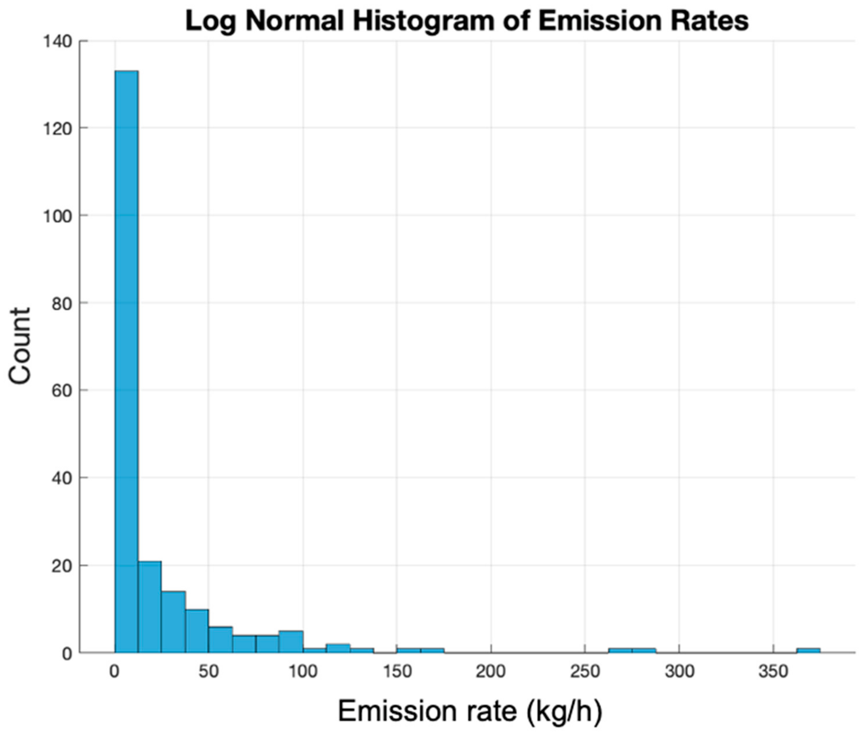
4]. To gain a greater understanding of current North Sea emissions, the Environmental and Emissions Monitoring System (EEMS) maintained by OPRED (Offshore Regulator for Environment and Decommissioning) (
https://www.gov.uk/guidance/oil-and-gas-eems-database, accessed on 14 April 2022) dataset was compiled. The majority of the emissions data reported in the EEMS dataset occurred below 13 kg/h but the data was log normal, with a max emission rate greater than 300 kg/h, as shown by the histogram of the real-world emission data in
Figure 1.
Previous work in this methane emission measuring arena includes aircraft, ground and UAV platforms where lidar sensors were used to measure column-averaged methane and trace regional plumes [
5]. Additionally, satellites are making their way into the methane emission measuring space as technology advances and private space companies lower historic barriers. One such example is the GHGSat-D, manufactured by GHGSat in Quebec, Canada, has quantified time average methane emissions from individual coal mine vents [
6]. Other UAV based methane emission work has included mapping of emissions without supplementary ground-based measurements of a sludge deposit at a wastewater treatment plant [
7].
Using a miniature methane spectrometer and long-endurance unmanned aerial vehicle (UAV), individual offshore oil and gas assets’ emissions can be measured [
8]. To accurately measure methane emissions in real time from assets in a large offshore oil and gas producing region, such as the North Sea, we worked with operators through the Net Zero Technology Centre (NZTC) worked together to use SeekOps small, lightweight sensor with unmanned long-distance UAV to quantify facility level emissions. The pairing of an accurate methane spectrometer sensor with an UAV allowed deployment from land to nine offshore platforms in the North Sea in 2020 and 2021, where operation interruptions were minimal and safety protocols were strictly adhered. Innovative flight patterns and novel algorithms developed to calculate mass flux from point concentration data around each asset in this study allowed for rapid processing time and demonstrated the use of this system to derive accurate facility-level emission rates to verify current industry performance and data and highlight discrepancies from traditional bottoms-up methods [
8].
The UAV-deployed quantitative gas detection solution described here has been field-proven, validated, and used to investigate methane emissions from a variety of sources including flare stacks, upstream and midstream fugitive emissions, and biogas/biomethane and landfill sites [
9]. The sensor is a laser-based miniature Mid-Wave Infrared (MWIR) spectrometer capable of detecting parts per billion level changes in methane concentrations at a sampling rate of 10 Hz. These measurements coupled with change-detection algorithms enables the identification of even very small emissions. Deployment via UAV allows the sensor to more efficiently survey areas that would otherwise be difficult or unsafe to complete using handheld or stationary sensors, saving time and money. Emissions sources are surveyed by flying downwind curtains, as guided by a ground anemometer, or perimeter polygon curtains around the entire area. When desired, the area can be broken in smaller pieces, or equipment groups, as is often necessary in landfill applications, which typically cover a larger acreage than a well pad or biogas facility. Once the methane measurements have been recorded, the data is uploaded and processed to give an emission rate estimation.
To better understand methane emissions from offshore platforms, we performed a remote methane survey of facilities in the North Sea. These flights served as the first comprehensive methane emissions survey of an offshore platform with a miniature methane spectrometer onboard a UAV [
10]. This new approach provided fit for purpose “top-down” emissions measurements required to meet the goals of emission data verification. The purpose of the project leading up to the 2020 campaign was to develop a method for detecting and quantifying methane emissions from any offshore facility globally. The approach measured site-level total methane emissions from either outside or within the operational exclusion zone of offshore facilities. Similar to onshore reporting, current offshore methane emissions reporting requires “bottom-up” accounting, which in well-metered instances are reported with a high degree of confidence but for unmetered sources can lead to significant uncertainty in the calculated emissions. With the advent of compact, low weight, sensitive sensors, high resolution aerial measurements, and innovative algorithms for emission rate calculation, this new technology is now available for accurate emissions quantification. The integration of these developments enabled quantification of emissions rates that can verify calculated bottom-up values and give the facility operator an improved understanding of their methane performance. Beyond the reporting implication of this approach, this method(s) may lead to early identification of emissions issues from a safe distance that are unobtrusive to normal operations.
2. Materials and Methods
The in situ methane sensor used in this work is a laser-based miniature MWIR spectrometer capable of detecting parts per billion level changes in methane concentrations. More detail on sensor performance can we read in Smith et al. [
8]. The sensor is designed to be either mounted in the bottom of a fixed-wing unmanned aerial vehicle (UAV) or mounted on the front end of a quadcopter drone, so readings are not influenced by the propellor wash out, as shown in
Figure 2. Use of a fixed-wing drone enables much longer duration flights than its rotorcraft counterpart and has allowed for unobtrusive long-range surveys of offshore assets to be conducted, whereas the use of rotorcraft allow greater resolution between equipment groups—allowing precise locations of emissions to be resolved. The choice of aircraft can therefore be made to reflect the type of emission data being obtained. The performance of the closed-cell methane sensor was characterized by multiple in-lab, ground, and flight tests.
A key aspect of the specific solution described here is a process for emissions rate quantification that is based on a standard engineering control volume model. There are three major contributions to this process: (1) the fast response in situ gas sensor, (2) an optimal flight pattern design, (3) proprietary analysis methods that allow for rapid and accurate quantification.
To survey methane from assets and platforms offshore, beyond visual line of sight (BVLOS) flights originating from shore (e.g., airfield, airstrip, airport) were conducted using a long-range UAV and the miniature laser spectrometer integrated below the flight surface. The preferred flight pattern designed to accurately survey methane emissions while accounting for flight limitations, such as flight time and range, was selected through a combination of plume modelling and flight path simulations [
8]. These simulations yielded an optimal flight envelope radius of 250 m and an altitude profile of 0–185 m. However, the optimal flight pattern was not always feasible due to the safety restrictions of assets. A normal exclusion zone is 500 m, but the UAV can be granted permission to fly closer when low emission rates are expected based on bottom-up averages. However, when a facility has floating components, a larger standoff distance may be used to allow for vessel movement around a central axis. Through closed surface flight paths such as these, flowrates can be calculated.
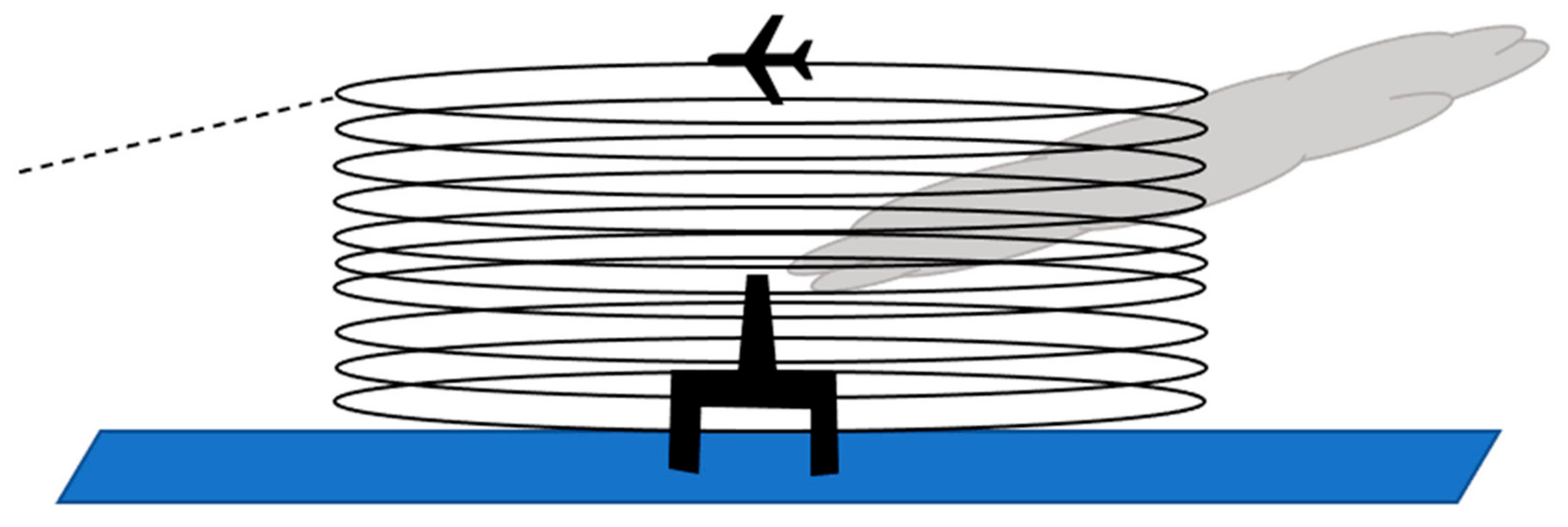
During our helix flight pattern, the fixed-wing aircraft flew at a constant radius around the asset’s furthest point from the center. A simplified schematic of the fixed-wing flight pattern is shown in
Figure 3. The aircraft started the testing event at the set radius from the asset being surveyed at the highest sampling altitude. Once at the set radius, the aircraft spiraled down in a counterclockwise pattern from the maximum altitude, ~210 m (700 ft) above ground level (AGL) stepping down at a consistent vertical step to the lowest altitude, usually around 30.48 m (100 ft) AGL at a constant speed of 30 m per second. Once at the lowest safe altitude, the aircraft will spiral up at the same altitude step in the counterclockwise direction flying between the previous laps, creating an interlaced track. Flying between the spiral down altitudes on the upward section of the flight path increases the vertical resolution of the data while limiting the time dependency of altitude and emission. This spiral down then immediate spiral up flight pattern will be referred to as “down–up” or DU for the duration of this document. With a standard standoff distance of 300 m and a drone speed of ~31 m/s, surveys usually take around 30 min to complete.
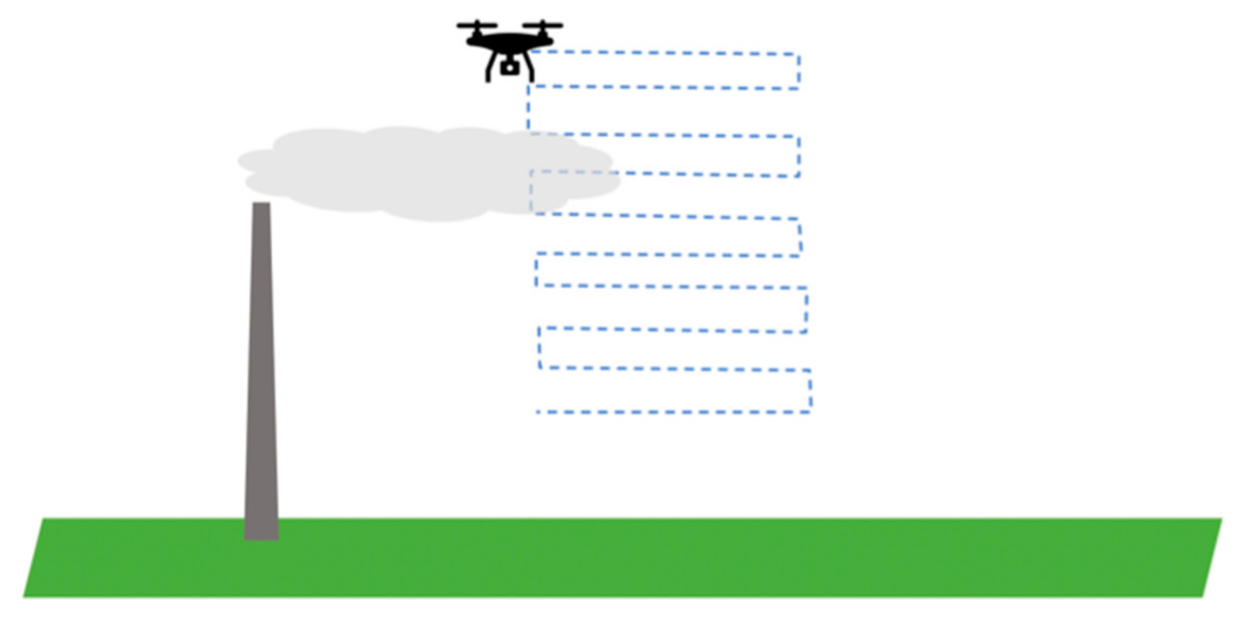
For the quadrotor drone, two flight patterns have been developed. The first involved the pilot flying the drone a safe distance downwind of a potential emission source, as determined by the safety guidelines and an anemometer. This flight pattern has been proven successful in controlled release and field campaigns [
11]. Once a plume is located using the streamed methane concentrations displayed on the ground control system, a curtain pattern was flown starting at the lowest altitude up to the highest to completely envelope any emissions as seen on the ground control unit and an immediate decent in the same area interlacing the ascent path. For a full survey, this pattern was flown twice.
Figure 4 shows a schematic of this flight path. These flight patterns are useful as they take a short amount of time to complete. They also require minimal flight planning and air traffic permissions due to the relatively short altitude range. Lastly, due to the impromptu nature, smaller areas can be isolated and surveyed individually, allowing for equipment group level estimations of emission rates. These flux plane or curtain-like flight paths usually take about 30 min to complete, depending on the horizontal length of the flight path. If the horizontal distance is large in the case of landfills, surveys can take a few hours to complete.
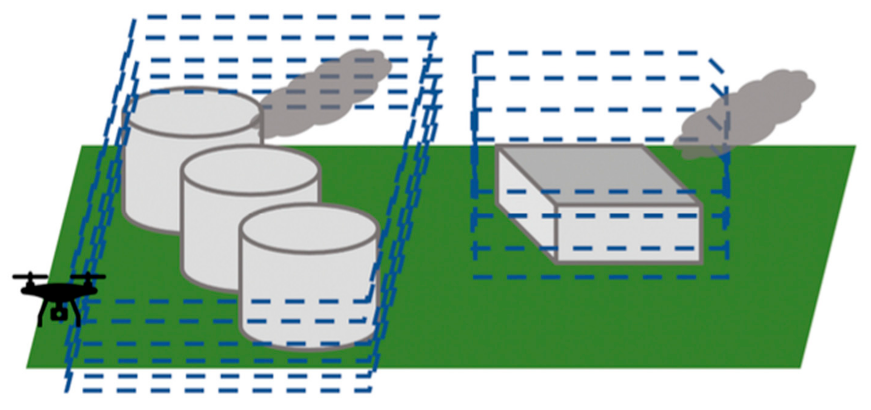
Another flight pattern deployed using the quadrotor drone has been termed the perimeter method, where polygons around the emission point were flown at altitude intervals creating a closed surface similar to the helix flight pattern used for the fixed-wing. The drone traced the polygons at ascending altitude heights and then descended, interlacing the altitudes flown during the ascent.
Figure 5 shows a schematic of the perimeter flight path. These flight paths guarantee quantifications from the survey are from within the perimeter sampled, limiting outside influence of neighboring emitters. Additionally, these flight patterns were automated and so are useful when comparisons over time are desired as they ensure the comparison is like to like. These types of flight patterns take longer to complete than the flux plane or curtains due to the linear distance needed to complete.
As mentioned previously in
Table 1, the sensor measures instantaneous methane mole fractions at a 10 Hz sampling rate. The helical mass flux emission quantification analysis method ingests volumetric mixing ratios and calculates the mass flux encapsulated in either the perimeter or the helix flight pattern resulting in a kilogram per hour emission rate of the encapsulated area, using a Lagrangian mass balance and Gaussian Theorem approach adapted from Nathan et al.’s paper that used a model aircraft to survey a compressor station [
12].
The mass balance approach was chosen over a classic Gaussian plume equation due to the dependence of Gaussian plume approaches on a large number of variables including stack height, stability class from the Pasquill–Gifford scale, wind profile exponent, stack temperature, stack tip diameter and stack velocity, requiring additional information and lot of involvement of operators of the sources of emissions [
13]. Operators may not record such variables at frequent intervals or be reluctant to provide such information; thus, Gaussian plume estimations would limit surveying potential and greatly increase the dependency of emitter involvement in the calculation of emissions.
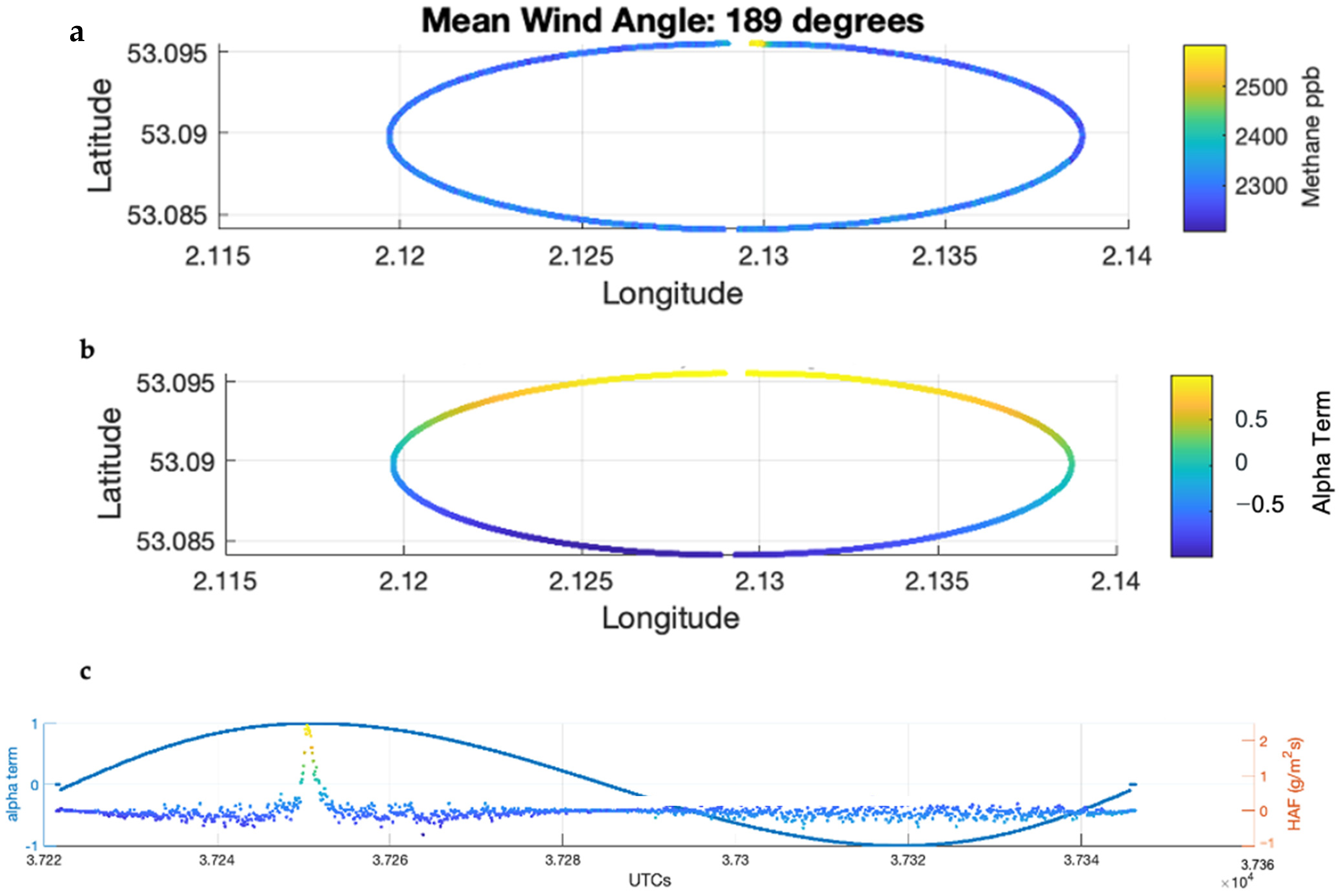
For the helix and perimeter flight patterns, data from the sensor methane sensor and the aircraft log files are recorded through the entire flight and then the individual laps are isolated around the emitter using algorithms that separate the laps around the emission source giving each lap a relatively uniform altitude and more individualized representation of the wind. The emission rate is calculated using Equation (1):
where the integrand is the path integral for each lap, or horizontal advective flux, where
is the mean horizontal wind speed during that lap derived from the UAV log files in the case of the fixed-wing, α is the angle relative to the mean wind at that sampled point in the lap such that at the most downwind moment, the alpha term, sinα, equals one and as the measurements are taken around the counterclockwise lap the alpha term slowly decreases until at the points directly upwind the alpha term equals −1.
is the density of air calculated using the ideal gas law with pressure and temperature of the air in the sensor measured at that point in the lap, and
is the methane mole fraction measured at that point in the lap. Without the account for real-world sampling effects, the summation of the alpha term around each lap equals 0; however, due to those real-world influences of sampling each methane measurement is not precisely equidistant and thus influences the lap integral. To account for this, the integral with constant methane concentration for the entire lap is subtracted from the integral of the methane measurements. Though this is a closed-loop integral, we use a smoothing
term to minimize any influence of sampling density (i.e., slight changes in speed of the UAV, instantaneous wind measurements, loop stepping) that would make the integral with a constant methane mole fraction not equal to 0. Due to the preprogrammed flight pattern and advanced flight tracking system, each lap is assumed to have equal vertical thickness. This assumption has been validated and any derivation from the equal height is minimal.
Figure 6 shows an example of a lap identified in the helix pattern where (a) shows the flight path colored for methane concentration in parts per billion, (b) shows the flight path colored by the alpha term, showing the area with the largest influence on the lap integral in the flight path is where the flight path is normal to the wind direction, (c) shows a time series in UTC seconds where the alpha term in plotted and the horizontal advective flux (HAF) in grams per meters squared seconds. As expected, the highest HAF occurs where the largest intersection of an emission is noted by the yellow color showing increased methane and the locational alpha term is also at the highest, denoting its most downwind location in the lap.
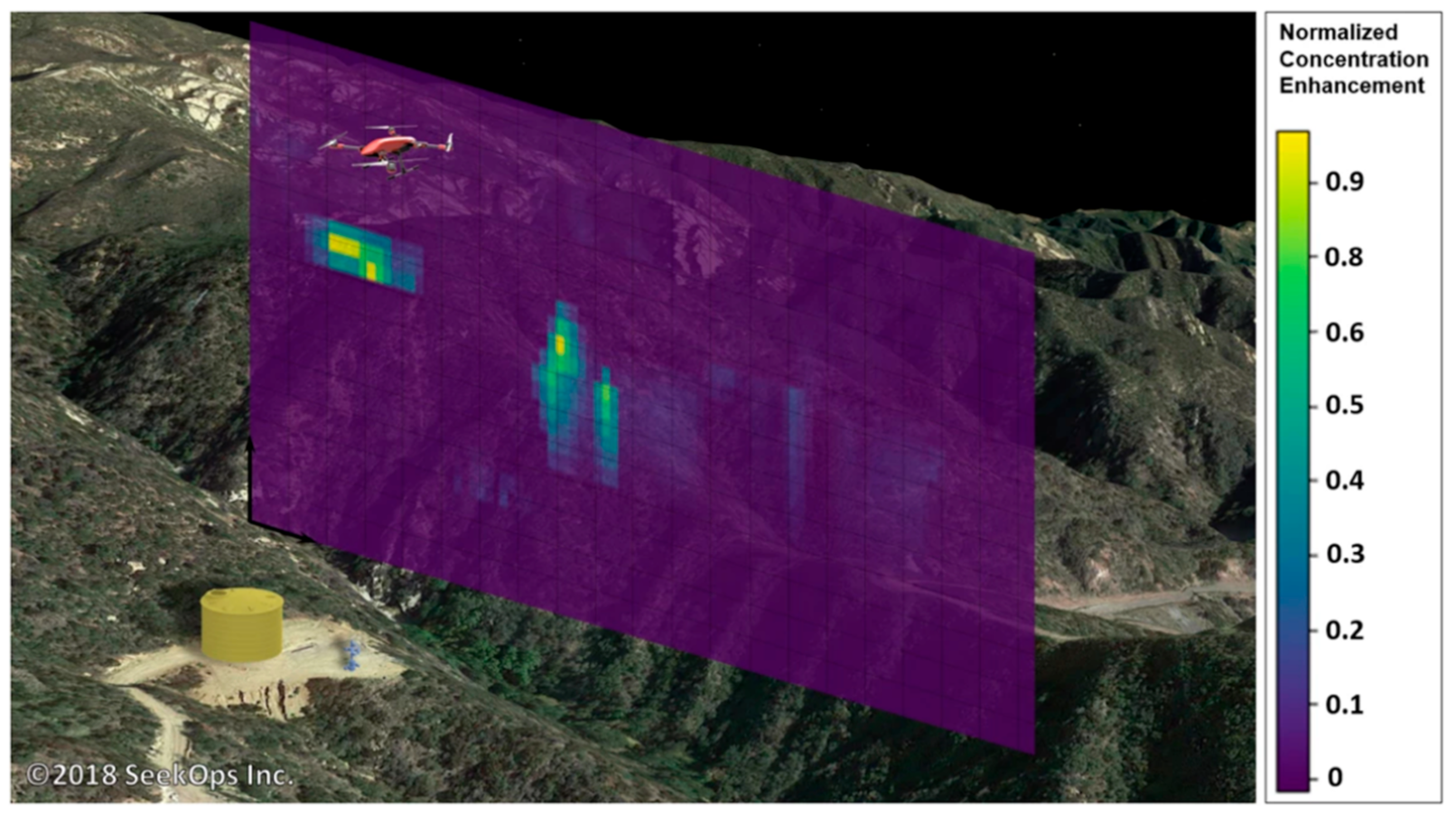
For the flux plane rotary drone flight pattern, data from the sensor methane sensor are recorded through the entire flight and then the individual curtains are isolated. A ground-based anemometer was set up on-site to measure wind speed and direction. Once the data is collected for a curtain, the data is interpolated onto a grid and projection to the normal of the mean wind direction as illustrated in
Figure 7.
Because we only measured the wind at anemometer height of 1.5 m, we used a standard log law vertical wind gradient equation to estimate the wind speeds at altitudes where the survey occurred not represented by the anemometer. The emission rate is calculated using Equation (2):
where
is the altitude binned wind speed using a ground-based anemometer and log wind profile estimation,
is the air density calculated using measured temperature and pressure,
average concentration measured in that grid cell, and
is the concentration measured in an upwind section of the survey.
Controlled release experiments were designed to gain a better understanding of the empirical uncertainty of the methods, and a more detailed appreciation of the assumptions that go into the analysis. The sensor had been validated and calibrated in a laboratory setting, but to understand the validity of these methods at quantifying methane emissions, we needed to compare the sensor deployment, processing algorithms, and techniques to a metered source. These controlled release experiments aided in the understanding of how well the flight patterns sample the plume, and how accurately the method calculates the emission rate at varied emission rates and flight radiuses.
The test objectives were as follows:
Determine the efficacy of emission detection for variable rates at different distances from the emission source;
Ensure the repeatability of flux calculation as the distance from the emission source is increased;
Ensure that the majority of the plume is accurately transected during flight patterns;
Verify the independence of emission rate estimate accuracy to the actual emission rate;
Define the empirical uncertainty of the methods by calculating the relative error of the actual release rate against the calculated rate.
The following variables in
Table 2 were either logged or controlled during the flights. A certified gas meter was used to verify emission rates throughout the tests and the methane supplied was lab certified and traceable with datasheets.
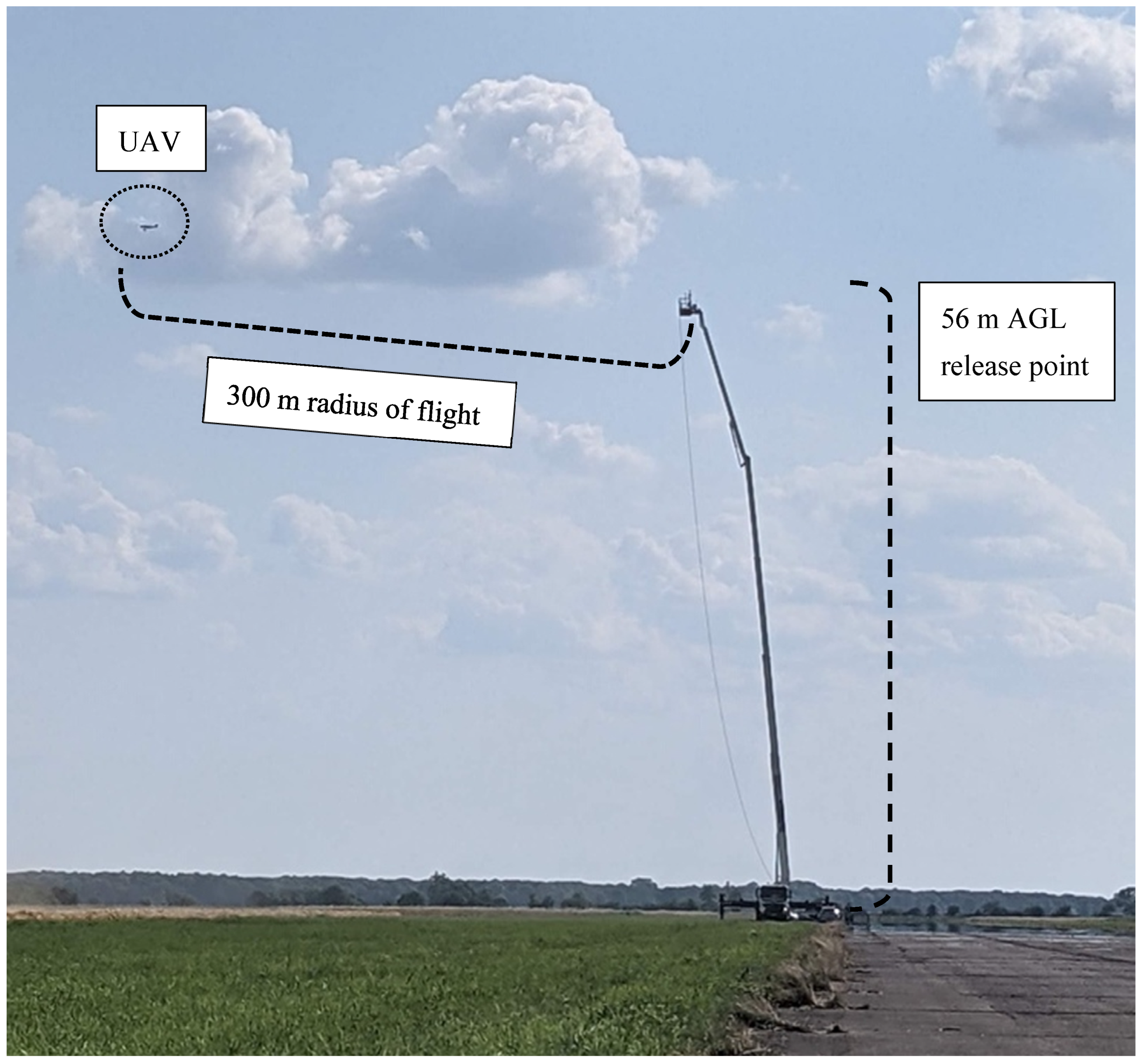
The controlled release experiment took place at Deenethorpe Airfield located 2 miles east of Corby, Northamptonshire, England where we were able to control aircraft in the region and adhere to strict airfield safety protocols. We used a mass flow controller with digital readings to control the flow of the methane at set points throughout the experiment.
To most mimic real-world emissions, a 56 m tall crane was used to elevate the release point, as shown in
Figure 8.
Table 3 outlines the fixed-wing UAV controlled release experiment, specifically identifying the emission flow rates, releasing CH
4 at 55 m (180 ft) height above the ground, flight pattern, step size (10 m or 25 m), and the date each testing event occurred. Test event order was chosen to limit any correlation between parameters outside of the experiment control, such as weather and wind, with measured sensor data.
Table 4 outlines the quadrotor UAV controlled release experiment, specifically identifying the emission flow rates, releasing CH
4 at 55 m (180 ft) height above the ground, flight pattern, and the date each testing event occurred. The test event order was chosen to limit any correlation between parameters outside of the experiment control, such as weather and wind, with measured sensor data.
4. Discussion
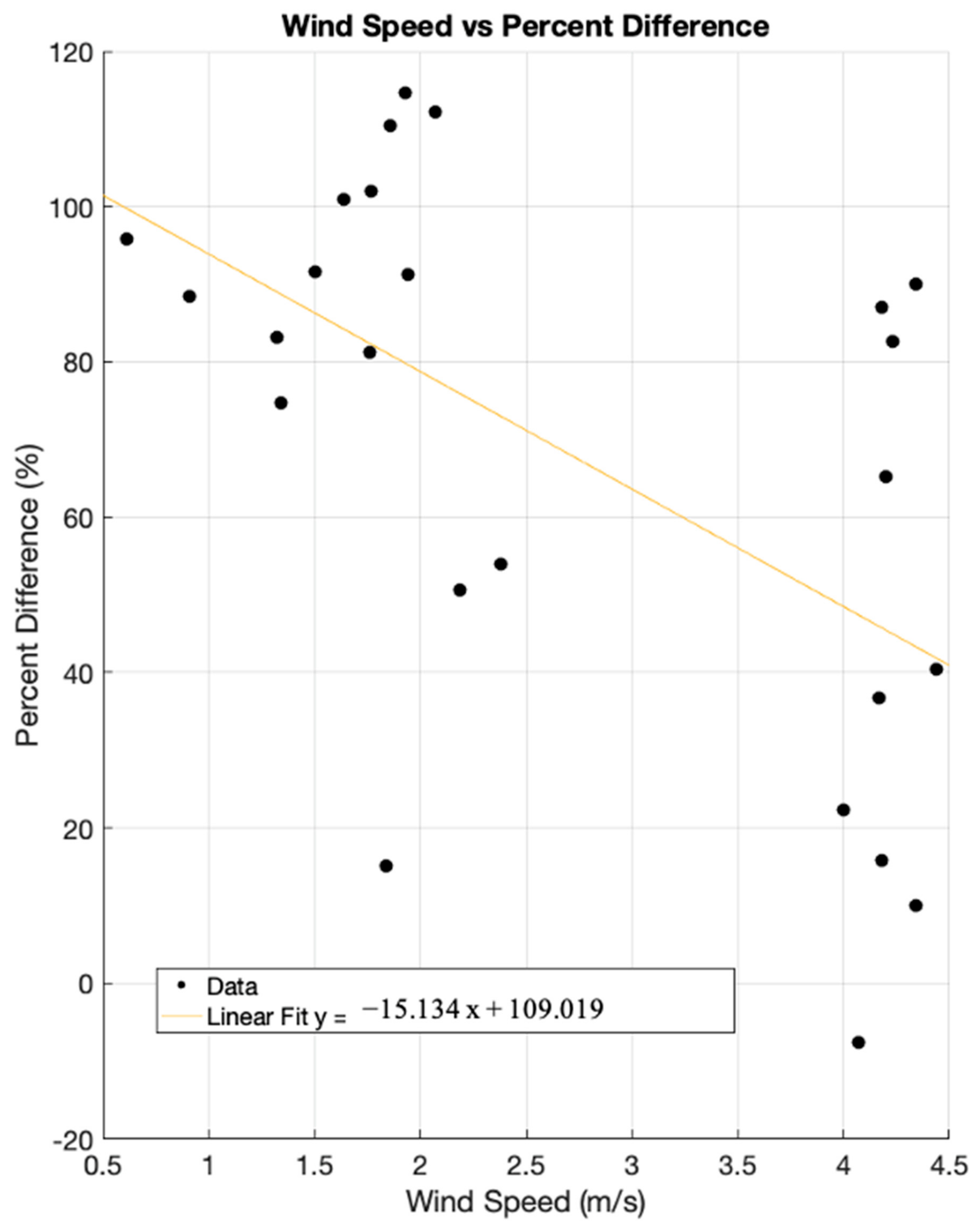
Atmospheric stability, or the tendency of the atmosphere to resist or enhance vertical motion and thus turbulence, is determined by wind speed, direction, and solar insolation where a potential temperature profile is not available. An unstable atmosphere enhances turbulence, whereas a stable atmosphere inhibits mechanical turbulence. For the lowest uncertainty, it is optimal to survey during neutral or stable conditions as proven by the increased uncertainty of the 18 fixed-wing tests in unstable conditions. Though we observed low winds and an unstable atmosphere in our experiment, we are unlikely to experience that in offshore environments. Atmospheric stability is generally more stable over water, where the water takes longer to heat and cool when compared to earth.
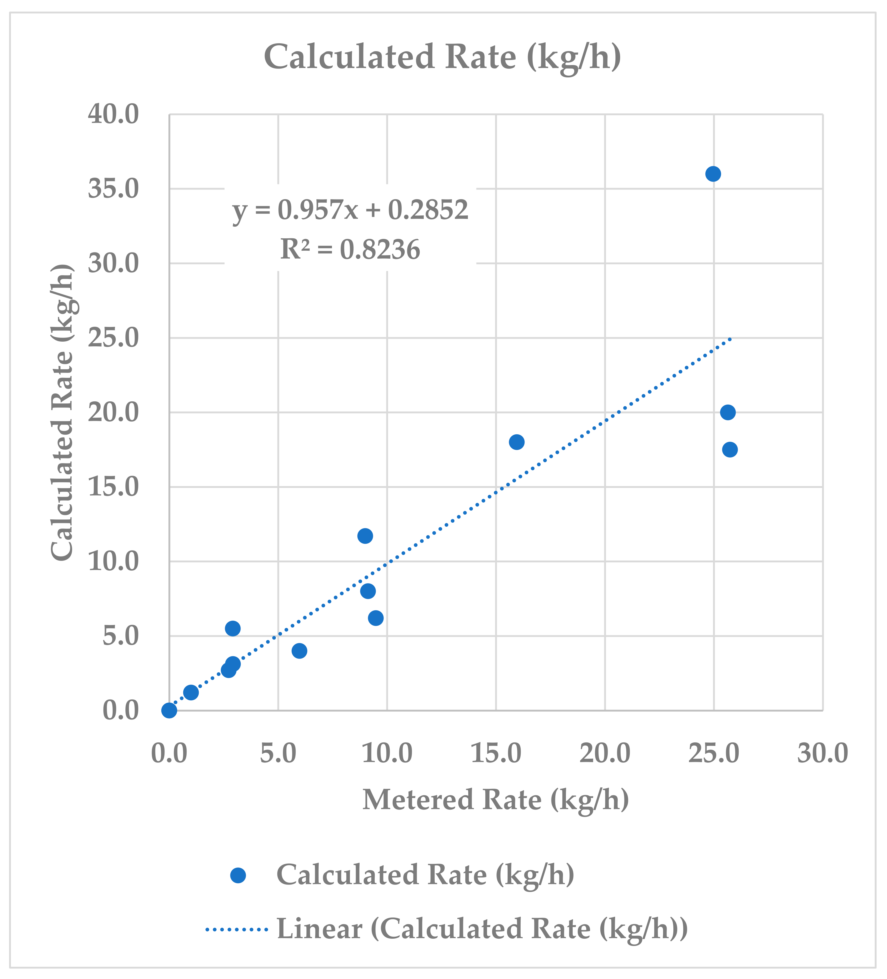
This experiment confirms the fixed-wing DU helix pattern at 300 m standoff distance intercepts the plume. The data shows that the sensor can perform accurately when compared to a metered emission source. The method calculated emission rates accurately (within ±16%) at higher atmospheric stability across the range of emission rates released (3–25 kg/h) when using the fixed-wing to deploy the sensor. This shows promising accuracies for offshore applications and applications when site access or very close proximity is not possible. The uncertainties in this experiment described the sensor, flightpath, and method(s) during mostly unstable atmospheric conditions, which are unlikely in usual surveying conditions for fixed-wing applications (primarily offshore). This experiment gave greater insight into how flight patterns and atmospheric conditions can affect our results, and we will use this knowledge in the planning of future surveys to ensure that uncertainties are minimized.
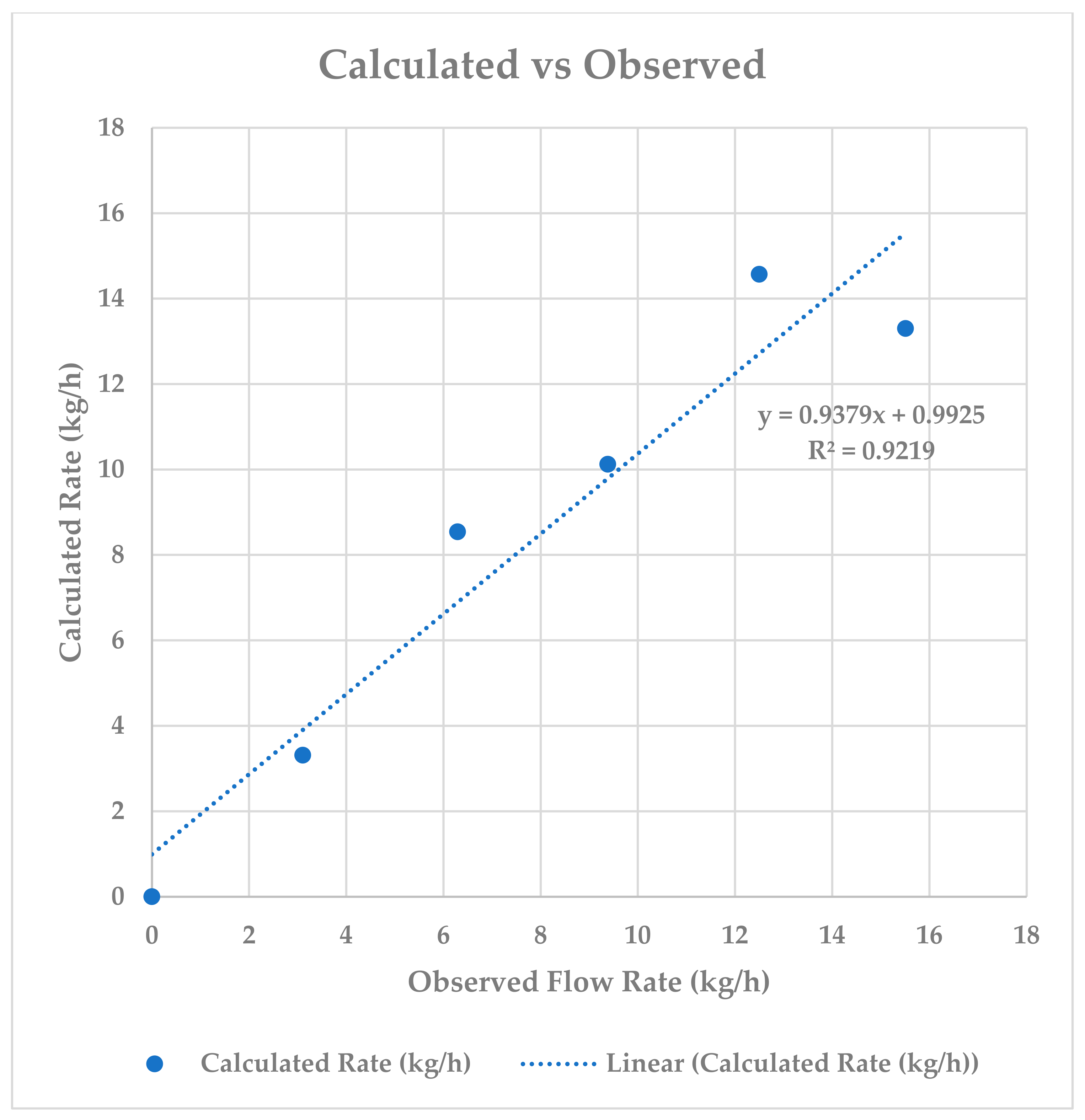
The flux plane flight pattern using the rotary drone, at both the 50 m and 300 m standoff distances, surveys the plume. The flux plane flight pattern, coupled with the previously described concentration to rate inversion method, accurately surveys emissions within 33% when full flights are performed and winds are greater than 1 m/s. The rotary drone is an accurate, reliable, flexible, and time-efficient alternative to a fixed-wing drone with a successful history onshore and has potential applications offshore, particularly when direct platform access is not practical.
5. Conclusions
Internal, regulatory, and societal pressures to limit methane emissions has in turn spurred innovation and technology development for measurement and mitigation of methane emissions. Simultaneously, large strides in unmanned aerial vehicle technology has enabled precision measurement in extreme environments (e.g., offshore oil and gas facilities). The oil and gas industry has a history of leading such innovations in measurement and participating in industry-wide efforts such as the Oil and Gas Methane Partnership (OGMP). OGMP pushes for accurate global accounting of emissions using best available technology and respecting the nuances of global operations, all while enabling a standardized approach that is not prescriptive. It is up to the industry to suggest appropriate methods and best practices that can meet the critical goals set forth by OGMP 2.0.
The lightweight, rugged in situ sensor in presented in this study proves that methane measurements can be collected in an operationally efficient and consistent manner that is appropriate for methane measurement and reduction goals of the industry. Furthermore, it is shown that leveraging small UAV technology is critical to methane emission reduction goals and can be used to not only detect methane emissions, but also robustly quantify them. Using empirically collected controlled release data, this work has highlighted that deterministic analysis of methane concentration measurements from a sensitive mobile spectrometer combined with wind data can yield accurate and robust asset-level emission rates from offshore oil and gas operations, and other methane emitting industries such as landfills and biogas.
Robust autonomous data processing procedures have been established allowing for a one-to-one comparison of repeat surveys, while guaranteeing that surveys fall within the accuracy and uncertainties described. This standardization of data acquisition and processing allows repeat surveys to be compared and compiled for greater understanding of asset emissions, as well as over time add to the statistics of similar sites and regions. The automated processing techniques used in this study allow for a short processing time, enabling near real-time actionable information and, therefore, facilitating faster remedial action. Faster remedial action and mitigation saves customers money all while limiting further emissions, benefitting the climate.
The standardized flight patterns used in this study adequately measure the methane emissions, take approximately 30 min to complete, and therefore offer minimal disruptions to assets normal operating procedure. With limited disruption, these surveys can be utilized at temporal intervals to gain accurate insights into not only facility-level emissions but also equipment group-level emissions in the case of the quad rotor applications. The sensor, standardized quantification methods, and automated algorithm suites perform accurately and consistently when compared to a metered emission source. This gives us great confidence in the method in quantifying emissions in the real-world applications, especially oil and gas production surveys that our experiment was designed to mimic. Additionally, this experiment gave greater insight on how flight patterns, intrinsically data density, and atmospheric conditions can affect emission quantification results. We use this knowledge in the survey planning to ensure the best results with the smallest uncertainties.
As industries continue to strive toward net-zero, new technologies such as those described in this work will continue to be developed an fill any gaps in industry knowledge. Accurate measurement of emissions is the first step to mitigating and reducing emissions. Using these methods, industries will be able to gain accurate emissions quantifications and reduce their emissions for the betterment of the global climate, all while deploying in a manner that is cognizant and meets the broader stakeholder interests.


