
Air Pollution Dispersion over Durban, South Africa


1
Physics Department, University of Puerto Rico, Mayagüez, PR 00682, USA
2
Geography Department, University Zululand, KwaDlangezwa 3386, South Africa
*
Author to whom correspondence should be addressed.
Atmosphere 2022, 13(5), 811; https://0-doi-org.brum.beds.ac.uk/10.3390/atmos13050811
Submission received: 8 April 2022
/
Revised: 5 May 2022
/
Accepted: 9 May 2022
/
Published: 16 May 2022
(This article belongs to the Special Issue Sources, Characterization and Control of Particulate Matter)
Abstract
:Air pollution dispersion over Durban is studied using satellite, reanalysis and in situ measurements. This coastal city of 4 million people located on the east coast of South Africa contributes 29 million T/yr of trace gases, mostly from transport and industry. Terrestrial and agricultural particulates derive from the Kalahari Desert, Zambezi Valley and Mozambique. Surface air pollutants accumulate during winter (May–August) and provide a focus for statistical analysis of monthly, daily and hourly time series since 2001. The mean diurnal cycle has wind speed minima during the land−sea breeze transitions that follow morning and evening traffic emissions. Daily air pollution concentrations (CO, NO2, O3, PM2.5 and SO2) vary inversely with dewpoint temperature and tend to peak during winter prefrontal weather conditions. Descending airflow from the interior highlands induces warming, drying and poor air quality, bringing dust and smoke plumes from distant sources. Spatial regression patterns indicate that winters with less dispersion are preceded by warm sea surface temperatures in the tropical West Indian Ocean that promote a standing trough near Durban. Statistical outcomes enable the short- and long-range prediction of atmospheric dispersion and risk of exposure to unhealthy trace gases and particulates. The rapid inland decrease of mean wind speed from 8 to 2 m/s suggests that emissions near the coast will disperse readily compared with in interior valleys.
1. Introduction
1.1. Background
Emissions from urban, industrial and agricultural sources produce poor air quality that degrades respiratory health (asthma, pneumonia) and ecosystem function (eutrophication) [1,2]. Air pollutants such as carbon monoxide (CO), nitrogen dioxide (NO2), ozone (O3), sulfur dioxide (SO2) and fine particulate matter (PM2.5) accumulate over South Africa’s Highveld [3] where coal-burning power stations emit >10 K T/km2 per annum [4]. In addition, regional smoke plumes from deforestation [5,6,7] and desert dust plumes [8] add to the local atmospheric burden in the dry season.
Durban, South Africa, has an economic mix of agriculture, industry and services, which generate over USD 80 billion per annum, supporting a population of 4 million that sprawls 80 km inland and 100 km along the coast (Figure 1a). Durban’s busy harbor is surrounded by numerous factories linked by a modern road network (Supplementary Figure S1) whose traffic emits ~400,000 T/yr of trace gases [9,10]. Local emissions >100,000 T/yr derive from petrol refineries, sugar and paper mills, agricultural burning, diesel transport and generators [2]. The subtropical climate is warm year-round (14–28 °C), and coastal winds are blustery but diminish inland. During austral winter there are <12 rain days and near-surface lapse rates are >−5 °C/km [11,12,13,14,15,16]. A background anticyclonic circulation induces a sinking motion [5,17] that is pulsed by eastward-moving troughs. Studies [18,19] analyzed the dispersion climate of Pietermaritzburg (29.6° S, 30.4° E) and found ~20 ppb peaks of SO2, PM2.5 (morning) and O3 (afternoon) during winter (May–August) owing to nocturnal inversions and calm winds over interior valleys.
Satellites measure near-surface atmospheric constituents [20] via passive radiometers such as the atmospheric infrared sounder (AIRS) and the ozone monitoring instrument (OMI). Trace-gas retrievals use ultraviolet absorption [21] while aerosol retrievals use near-infrared absorption. Ref. [22] describes favorable validation of satellite NO2 and PM2.5 with in situ stations, whereas retrievals for SO2 are less certain under dust, smoke or clouds—as shown later. Emission plumes can be narrow [23] so in situ measurements exhibit large spatial and temporal variance [24]. If monitoring stations are located close to emission sources, meteorological influences can be distorted [17]. Data assimilation of satellite and in situ observations, together with emission inventories and meteorological measurements by global air chemistry reanalysis [25,26], overcomes many limitations and enables a remote study of urban air pollution [27].
1.2. Motivation and Objectives
Air pollution over big cities of developing countries is estimated to cause millions of premature deaths and billions in economic losses per annum [28,29]. South Africa’s subtropical climate accumulates air pollution that leads to health impacts and acid rain (pH ~ 4) [30,31]. Durban contributes 29 million tons per year of CO2 “equivalent” trace gases, mostly from transport and industry [32]. Thus, we are motivated to understand and predict the dispersion of urban air pollution.
Here we analyze trace gases and particulates over Durban, South Africa to understand meteorological controls on atmospheric dispersion from inter-seasonal to hourly timescales using satellite/reanalysis and in situ datasets. We address the following questions: (i) what induces inter-annual to multi-day variability of winter air pollution? (ii) do spells of high air pollution relate to certain weather patterns? (iii) which meteorological parameters best correlate with air pollution constituents across seasonal to hourly time scales? and (iv) can statistical links between prior climate and dispersion be utilized in air pollution warnings?
2. Data and Methods
2.1. Data
MERRA2 air chemistry data assimilation [25,33] yields continuous CO, O3, PM2.5 and SO2 concentrations in the surface layer: 1000–975 hPa, which covers elevated terrain west of the city. Satellite (‘s’) measurements from AIRS, MODIS and OMI provide aerosol optical depth (AOD) and surface-layer CO, NO2, O3 and SO2 [34,35,36]. Gaps in satellite data are reduced by applying a 3-day running maximum. We form an air pollution index (API) for the “Durban-area”: 30°–29.5° S, 30.5°–31° E, shown in Figure 1a, converting values to ppb then adding CO + NO2 s + O3 + PM2.5 + SO2 to obtain the cumulative concentration (Σ ppb). The surface API combines primary and secondary trace gases and aerosol particulates to underpin our study of atmospheric dispersion over Durban. Although MERRA2 has generated continuous information on local air constituents since 1980, the monthly and daily analysis starts in 2001 and 2005, respectively, in recognition of key satellite measurements.
Hourly in situ (‘i’) PM2.5 and SO2 are obtained from four stations: Pietermaritzburg, Settlers, Wentworth and City Hall of the Durban air quality monitoring (DAQM) network [37] shown in Figure 1b. These achieved only 60% coverage since 2001 and so are confined to mean diurnal and case study analyses. Regional aerosol particulate contributions from terrestrial dust (PM2.5) and agricultural smoke plumes are derived from MERRA2.
Meteorological data derive from CFSr2, ERA5 and MERRA2 reanalysis [38,39,40] and include air and dewpoint temperature, wind velocity, specific humidity, sensible heat flux (H flux) and planetary boundary layer (PBL) height or mixing depth. Comparisons between the datasets found interchangeable results, except for minor discrepancies of sensible heat flux. ERA5 is preferred for characterizing atmospheric dispersion, having 25 km resolution and being independent from air chemistry assimilation via MERRA2.
Statistical tests employ the same 0.5 × 0.5° Durban-area for extraction of time series. Cross-correlations of surface air constituents with meteorological parameters determined that a 1000–850 hPa layer average best represents transport and dispersion over Durban. Hereafter we refer to surface constituents and near-surface weather. Lapse rate ‘delta T’ is calculated as 850 minus 1000 hPa air temperature. Table 1 summarizes the dataset acronyms and characteristics.
2.2. Temporal Methods
To quantify east–west gradients in dispersion, winter (May–August) mean longitude slices are calculated on 29.75° S from 28.8°–31.9° E for ERA5 wind speed, sensible heat flux and PBL height. Daily ERA5 wind speed and direction scatterplots are made to highlight differences in air pollution transport at Pietermaritzburg and Durban Bluff (2005–2020). Histograms of daily wind speed and direction are analyzed for frequency distribution in winter (May–August 2005–2020). The mean annual cycle of the Durban-area API, ERA5 dewpoint temperature and KwaZuluNatal (KZN) provincial respiratory mortality [42] is calculated from 20 years of monthly data. It is noted that winds alternate during the passage of low- and high-pressure cells, so monthly vector averaging under-represents emission transport. The winter mean diurnal cycle analysis uses hourly in situ air constituents and ERA5 meteorological data (May–August 2011–2015, N > 104) focuses on land−sea breezes and Tmax–Tmin air temperatures. Intercomparisons were made of hourly reanalysis and weather station data at 29.8° S, 30.8° E, 512 m in July 2015.
The statistical analysis focuses on pair-wise temporal relationships between individual air constituents, the cumulative API and local meteorology. We apply Pearson product-moment cross-correlation to monthly, daily, mean diurnal and hourly (episode) time series. A multivariate regression is conducted between the daily API and all 14 weather parameters. After step-wise reduction of insignificant parameters, two are retained. Our sample sizes vary: 240 months (2001–2020), 5844 days (2005–2020), 24 h (diurnal 2011–2015), and 360 h (10–24 July 2015). Statistical significance at 90% confidence is evaluated by the degrees of freedom (deflated for persistence). The appropriate thresholds are r ≥ |0.36| monthly, |0.16| daily, |0.73| diurnal and |0.41| hourly.
2.3. Spatial Methods
To characterize the geography, we form maps of topography, MODIS mean temperatures and model surface roughness. To understand inter-annual variability, the monthly API time series is regressed onto May–August 2001–2020 (winter) fields of 200 hPa geopotential height, 850 hPa zonal wind, SST and satellite net outgoing longwave radiation (OLR) as a proxy for cloudiness. The point-to-field correlation maps quantify regional controls on year-to-year fluctuations of winter air pollution dispersion (N = 20). Similarly, we regress the daily API time series onto May–August 2005–2020 fields of SLP at one-to-three-day lead time (N = 1920). After ranking the top-10 API days, we calculate composite maps for near-surface winds and temperature, 500 hPa geopotential height and wind anomalies and vertical sections of zonal circulation and specific humidity on 29.75° S, 28°–32° E. A cluster of high API values occurred in July 2015, so we analyze the mean winds and PBL height and calculate twice-daily forward trajectories of virtual emissions from Durban via HYSPLIT ensemble simulations [43]. We also employ HYSPLIT dispersion simulations for time-of-arrival of industrial plumes from the Highveld on days with high API values.
2.4. Case Study and Prediction
A case study on 10–24 July 2015 emerges from hourly in situ air constituent measurements. MERRA2 air temperature and specific humidity are analyzed in time-height over those two weeks. Cross-correlations are computed for hourly air constituents, vector wind, air temperature, specific humidity, sea level pressure (SLP) and delta T (N = 360). We analyze a north–south vertical section of CALIPSO satellite particulates [44] on 12 July 2015. A vertical section (29.75° S, 28°–32° E) is plotted of the zonal circulation and AIRS satellite CO concentration. Maps of MERRA2 terrestrial dust and “black carbon” smoke plumes are analyzed for 15–16 July 2015. SAWS radiosonde profiles are obtained at Durban airport for 00:00 and 09:00 UTC 16 July 2015 to study night- and day-time airflow and thermal stability in the layer 1000–850 hPa.
To develop a forecast capability, we regress the winter API onto a variety of regional climate fields in the preceding summer (2001–2020). We found a statistically significant association with West Indian Ocean (WIO) sea surface temperatures (SST) averaged 20° S–10° N, 40°–85° E. We calculate lead/lag correlations from −12 to + 6 months with respect to the winter API to determine whether this association is steady and significant.
We generate outcomes from monthly to hourly time scales and present spatial regressions that demonstrate how the regional climate and local weather affect air pollution dispersion over Durban.
3. Results
3.1. Geography and Climate
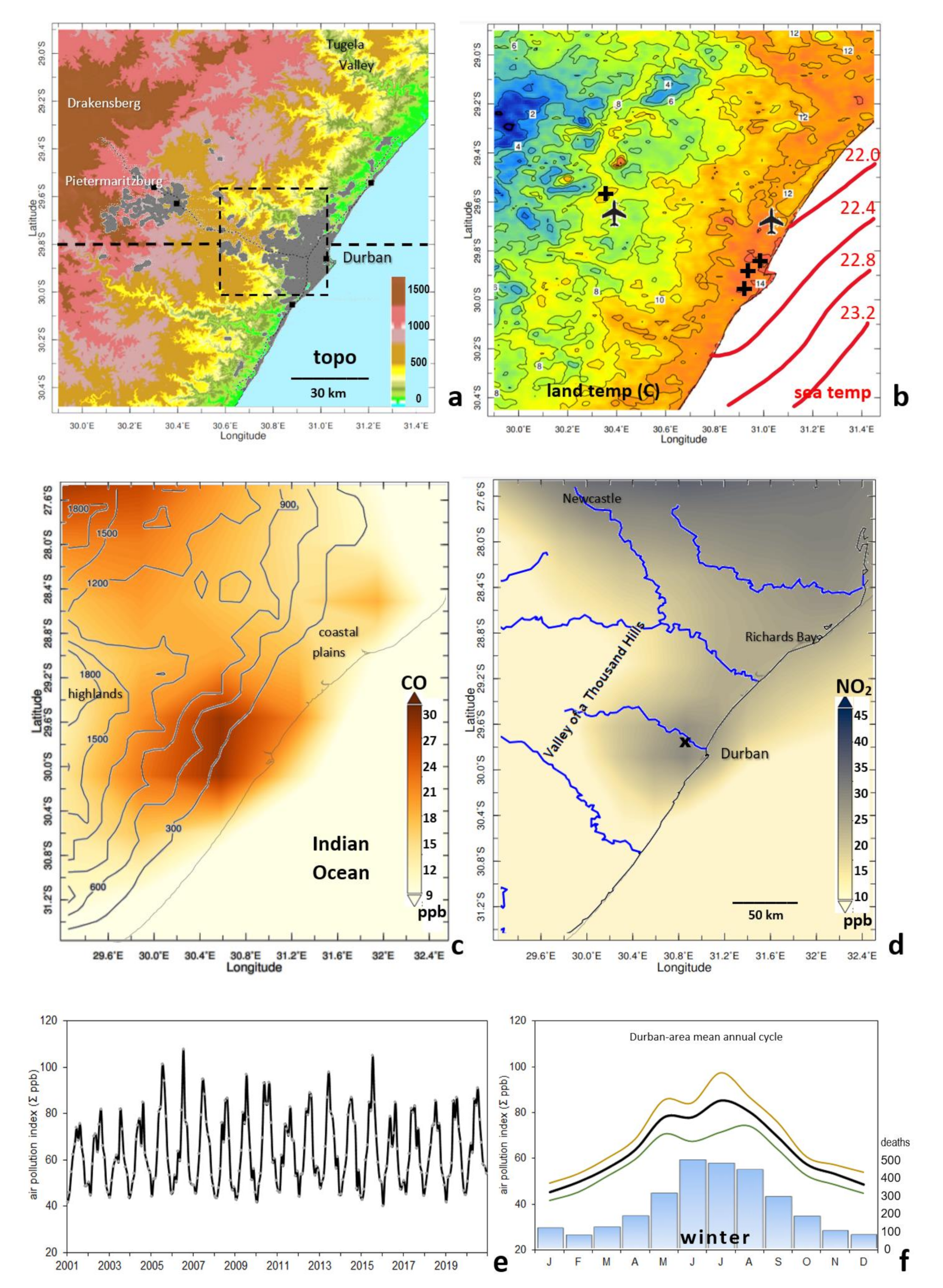
The coastal plains of Durban, South Africa align SW–NE and rise westward to the Drakensberg escarpment >1000 m. Several rivers cut through the Valley of a Thousand Hills forming a basin around Durban (Figure 1a). Winter night-time land temperatures (Figure 1b) decrease rapidly westward; offshore sea temperatures are ~22 °C.
Maps of mean surface-layer CO and NO2 concentrations (Figure 1c,d) show a hot-spot near Durban (~29.75° S, 30.75° E) as expected. Urban emissions from traffic, commercial and residential activities mix with industrial emissions from coastal refineries and factories, and with agricultural burning and power station plumes farther inland. Continental particulates are drawn from the Kalahari drylands and Zambezi smoke plumes far to the northwest [45]. The mean CO and NO2 maps reflect moderate concentrations in the sector 0–45° associated with the Newcastle and Richards Bay emissions. Conversely, the marine air mass in the sector 180–225° is clean. The satellite-measured hotspot is farther inland than simulated by [2,4]. The discrepancy may be due to the 25–50 km horizontal resolution and ~1 km depth-averaging of satellite retrievals. Yet we believe it represents reality based on emission inventories, air chemistry and meteorology data assimilation that accounts for dust and smoke plumes and stagnation in the Valley of a Thousand Hills.
The Durban-area monthly API time series and mean annual cycle (Figure 1e,f) reflect moderate air pollution levels that tend to peak in May–August each year, particularly in dry winters. There is a weak upward trend in the cumulative API record (+0.15 ppb/yr). Wavelet spectral analysis of the API with seasonality removed (Supplementary Figure S2b) highlights 2.5 yr and 5 yr periods that relate to predictability (cf. Section 3.8). Table 2 shows that CO, NO2, O3 and SO2 time series are significantly cross-correlated, whereas AOD and PM2.5 tend to be noisy. Trace gas concentrations reach a seasonal peak during stagnation in May–July, whereas aerosol particulates peak in August–September under windy conditions. Higher pollution concentrations occur under low humidity, westerly winds, negative sensible heat flux and shallow PBL height. Poor dispersion during winter coincides with airflow from the Drakensberg, leading to higher respiratory mortality from May–September (Figure 1f).
3.2. Coastal Gradients
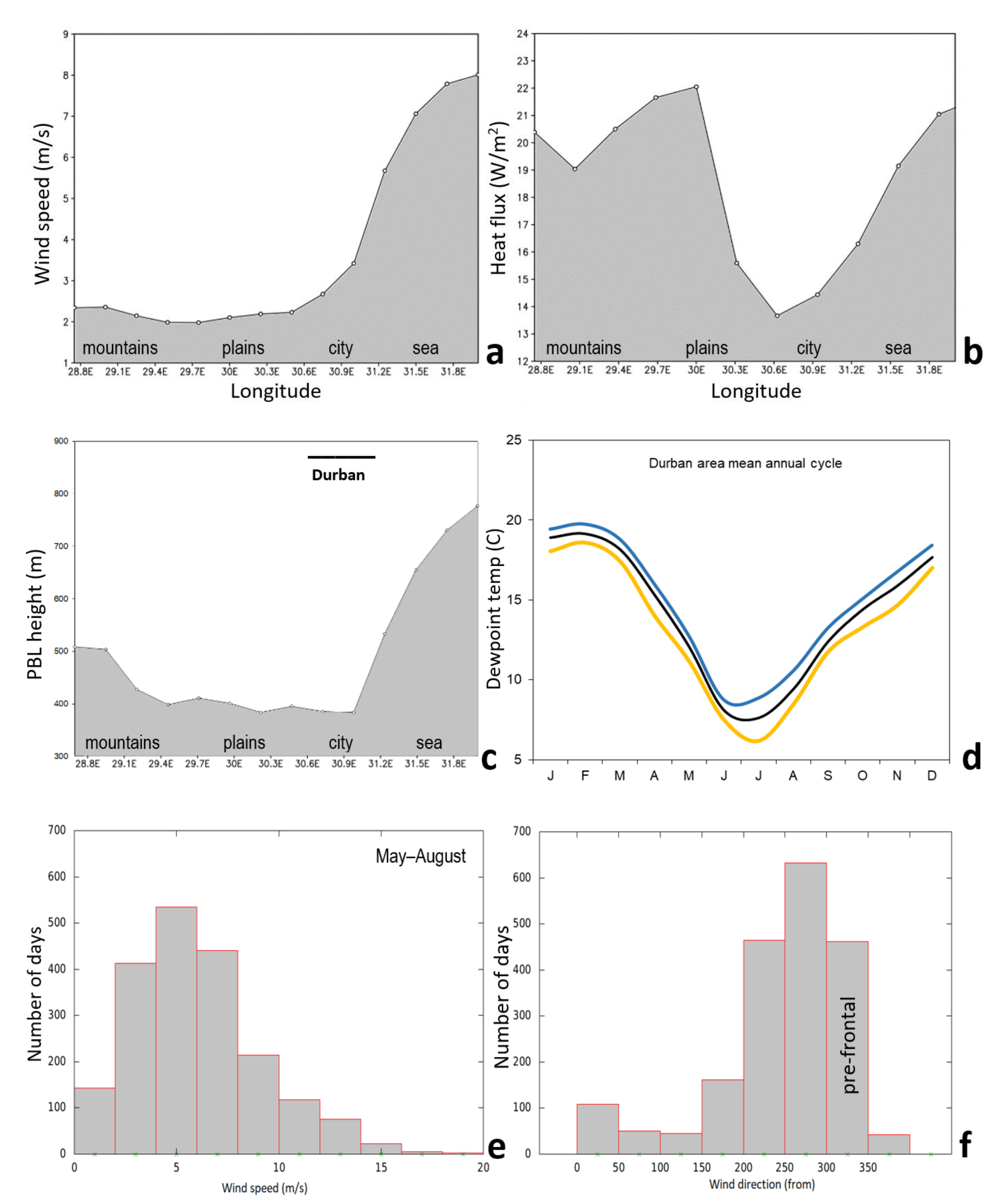
The annual cycle of dispersion and its coast-inland gradients are the focus of Figure 2a–f. East-west gradients are evident in long-term winter means on 29.75° S. ERA5 wind speeds and PBL height rise steeply to the east, where marine airflow averages 8 m/s and PBL height exceeds 700 m. In contrast, the interior valleys and plains have a shallow PBL height <400 m and ~2 m/s mean winds. Thus, emissions near Pietermaritzburg may recirculate while coastal emissions form SW or NE plumes depending on the prevailing weather. Sensible heat fluxes are generally low during winter, averaging 12 W/m2 over the Durban area and >20 W/m2 over the interior highlands and warm sea. As a result, a sizeable diurnal cycle emerges over the Valley of a Thousand Hills (cf. Section 3.5).
The mean annual cycle of dewpoint temperature (Figure 2d) reveals a steep decline from a January–February maximum of 19 °C to a June–July minimum of 7 °C. This seasonality reflects the advance and retreat of marine air induced by summer sea breezes and winter land breezes, respectively. The histograms (Figure 2e,f) indicate that area-height- averaged winds <4 m/s and prefrontal directions (300–350°) corresponding with poor atmospheric dispersion occur one-quarter of the time during winter. By contrast, surface winds on the coast are channelized SW−NE (Supplementary S3b) [46].
3.3. Inter-Annual Regression Patterns
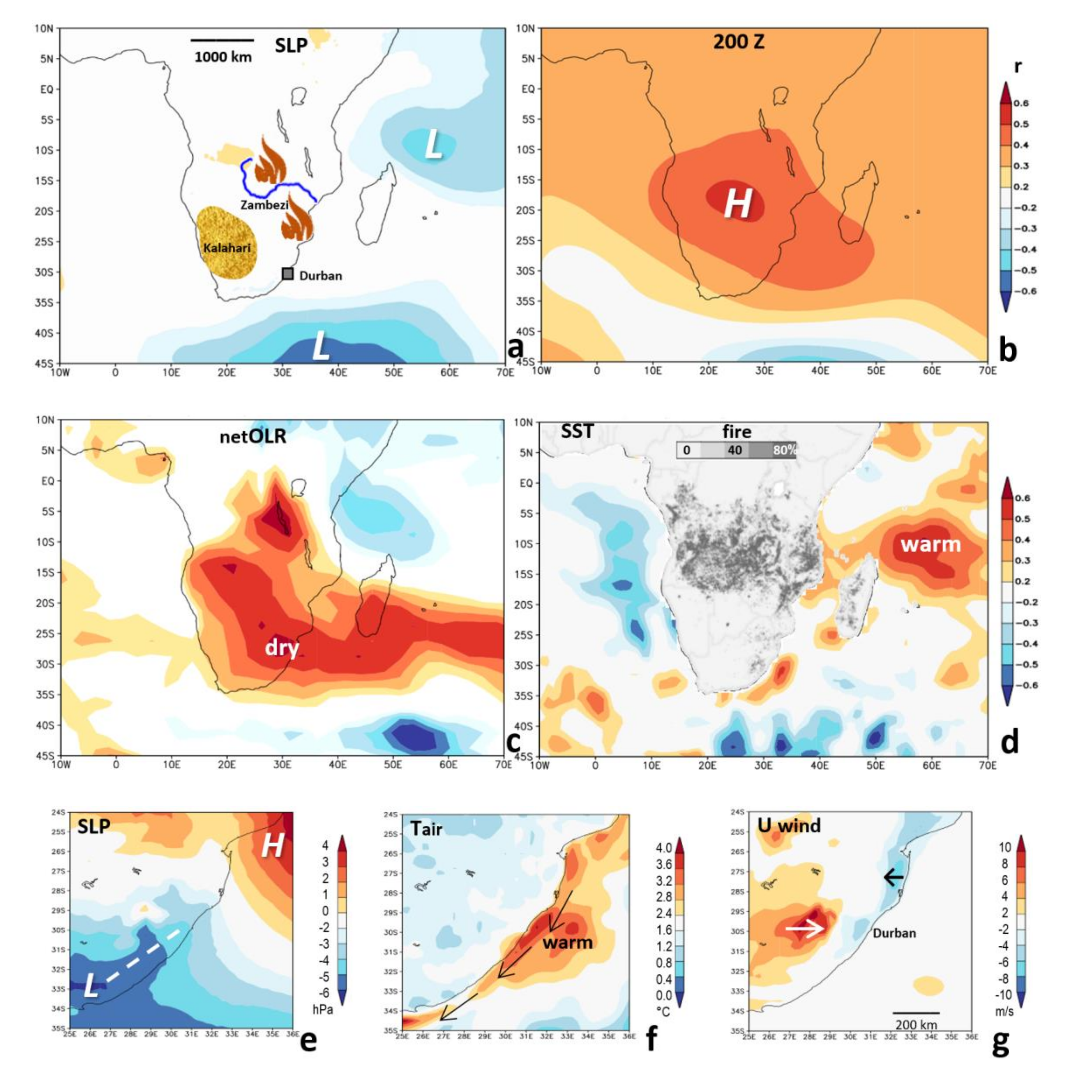
Regressing the May−August Durban API time series onto various fields, we find lower pressure in the mid-latitudes south of Durban, enhancing westerly airflow (Figure 3a). Negative SLP correlations are also found over the tropical WIO. The 200 hPa geopotential height (Figure 3b) correlations show higher pressure over tropical Africa and troughs at 0° E and 60° E in the mid-latitudes. Together these induce anticyclonic curvature of the subtropical jet over Durban during winters with high air pollution. The net OLR pattern (Figure 3c) reflects a warm, dry anomaly extending across southern Africa that helps generate dust and smoke plumes [47,48,49,50]. Sea surface temperature regressions with the winter API (Figure 3d) reveal a significant warm anomaly in the tropical West Indian Ocean.
Local regressions enable a mesoscale assessment of the dispersion climate. In Figure 3e–g we note that a trough penetrates from the Eastern Cape toward a ridge in the Mozambique Channel, yielding a low–west/high–east pressure gradient during winters with higher air pollution. Warmer marine air temperatures (>3 °C) draw land breezes from the Drakensberg (U > 6 m/s), promoting subsidence inversions that accumulate air pollutants. East coast (U < −3 m/s) sea breezes induced by the Mascarene High (with respect to API) suggest converging airflows that concentrate trace gases and aerosol particulates.
3.4. Daily Statistics and Weather Patterns
Daily statistics listed in Table 3 for the period 2005–2020 reveal that most air constituents are significantly cross-correlated, especially CO and O3 (r = 0.62). SO2 is weakly associated likely because of dust and smoke contamination in satellite retrieval and the intermittent nature of in situ measurements. Dewpoint temperature and near-surface humidity are negatively related to NO2 and O3 (r = −0.45 to −0.55). Near-surface westerly winds accumulate air pollutants (+r), while CO is sensitive to delta temperature. Local SLP has been deemed a predictor in earlier work [51], but at a daily time-scale its correlation is weak and positive for O3 and NO2 (r = 0.14 to 0.20). The pair-wise relationships enable inferences on meteorological controls of air pollution dispersion, with the API most affected by dewpoint temperature, humidity and zonal wind. Multivariate regression of the daily API onto all weather variables determined that 1000–850 hPa zonal wind and delta temperature were more significant.
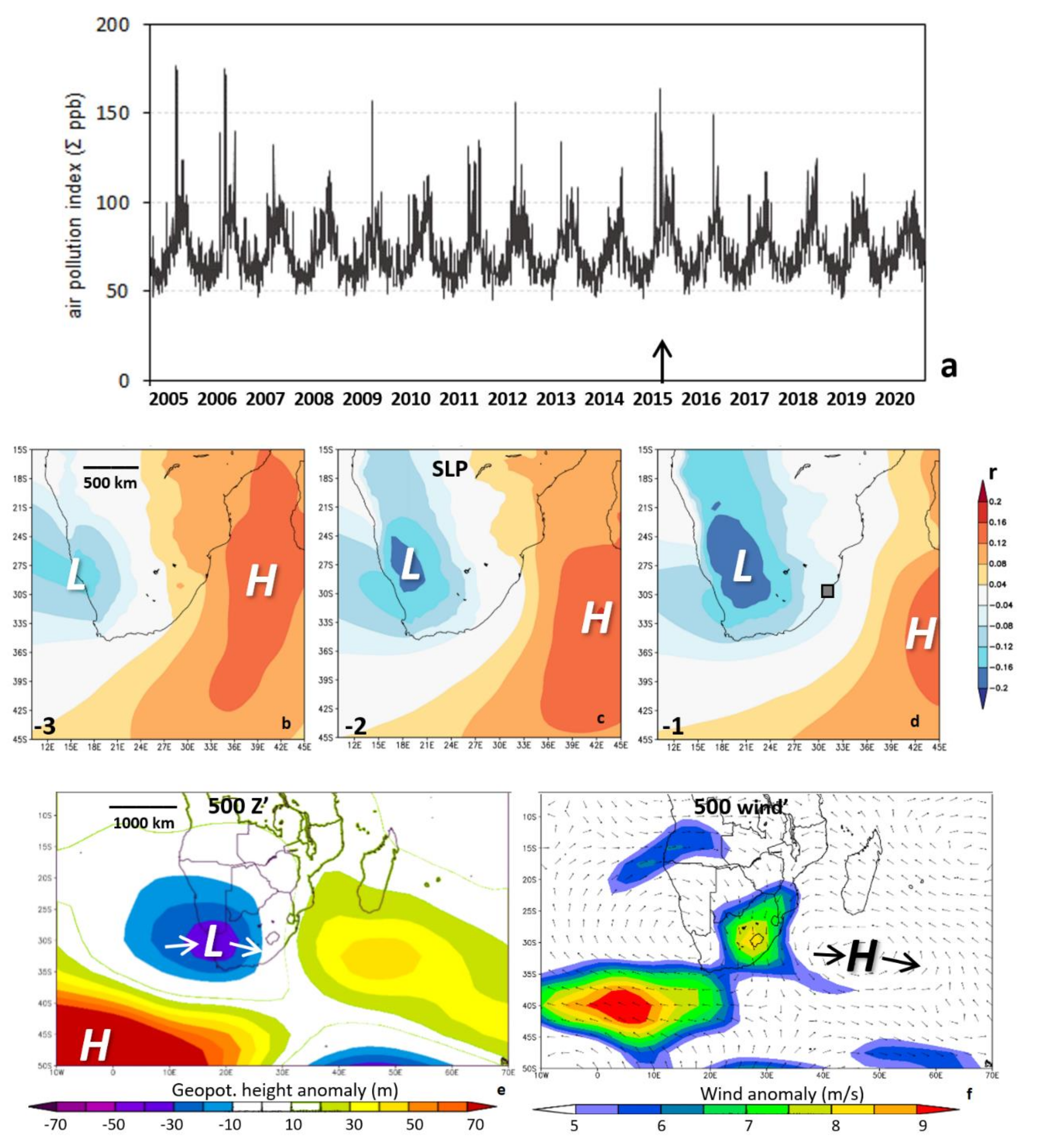
The daily API time series (Figure 4a) reveals a spiky seasonal character, with concentrations rising between May and September. Extended peaks occur in early June and mid-July because of local trace gases and during September under regional dust and smoke plumes that increase particulate loads. Daily API values remain low in the rainy season from November to April, as sea breezes draw marine air onto the coastal plains and wet deposition cleans the air.
Point-to-field correlations (May–August 2005–2020) with respect to the daily API reveal a low–west/high–east SLP pattern one to three days before high air pollution in Durban (Figure 4b). The pressure cells drift southeastward while generating large-scale poleward airflow. A similar pattern emerges via composite anomaly maps for the top-10 air pollution days (Figure 4c,d). The 500 hPa Kalahari trough and Mascarene ridge induce berg winds that accumulate air pollutants [14].
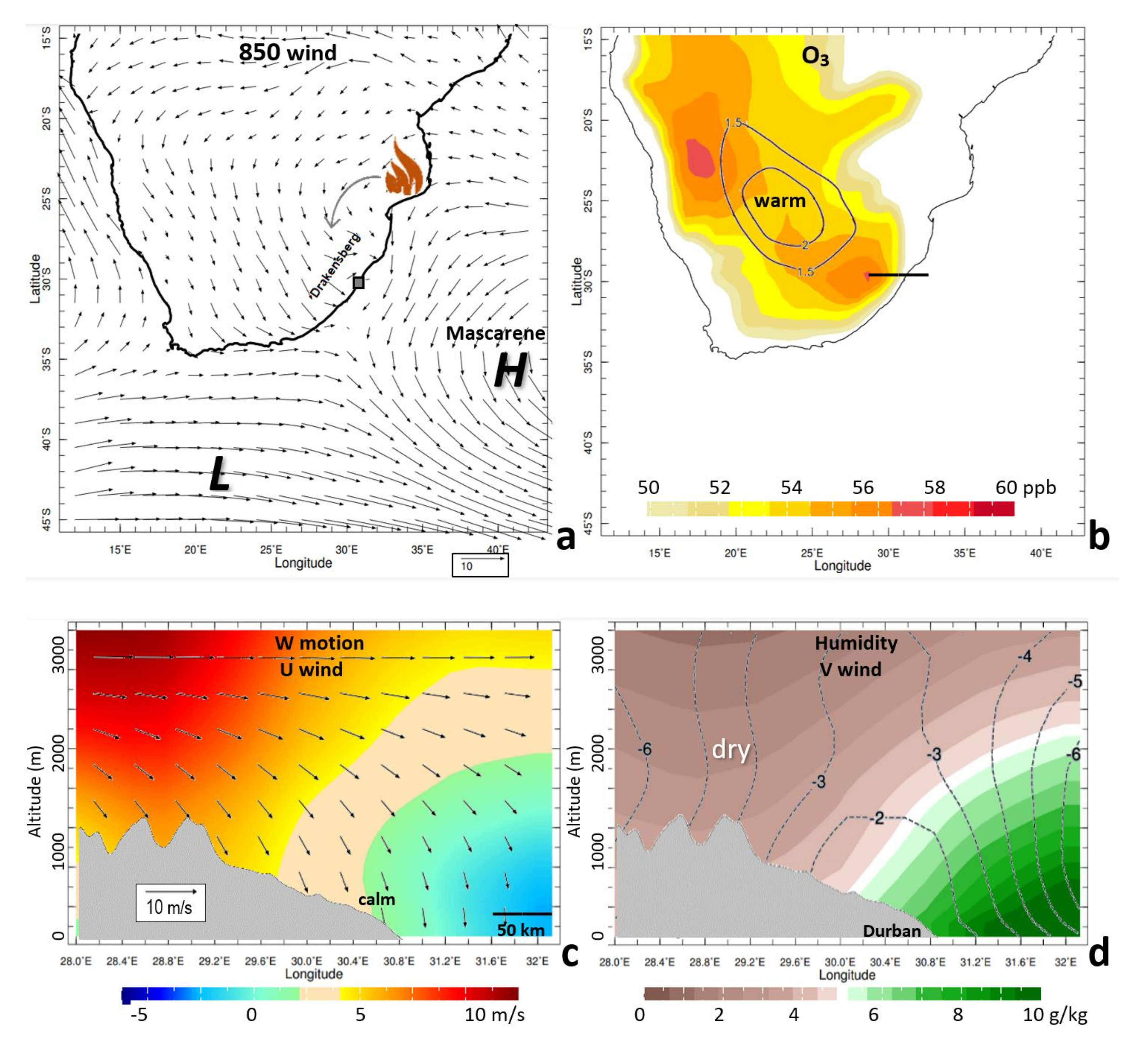
Composite near-surface winds for the top-10 days (Figure 5a) illustrate prefrontal weather corresponding with the low–west/high–east pattern. Smoke plumes from the Zambezi Valley and Mozambique join the airflow, causing high ozone concentrations (Figure 5b). Warm air temperatures and strong NW winds over the Kalahari Plateau cause a dust plume that is drawn toward Durban. The composite vertical section (Figure 5c,d) illustrates dry westerly flow aloft, a calm zone around Durban and humid easterly flow offshore.
3.5. Diurnal Cycle during Winter
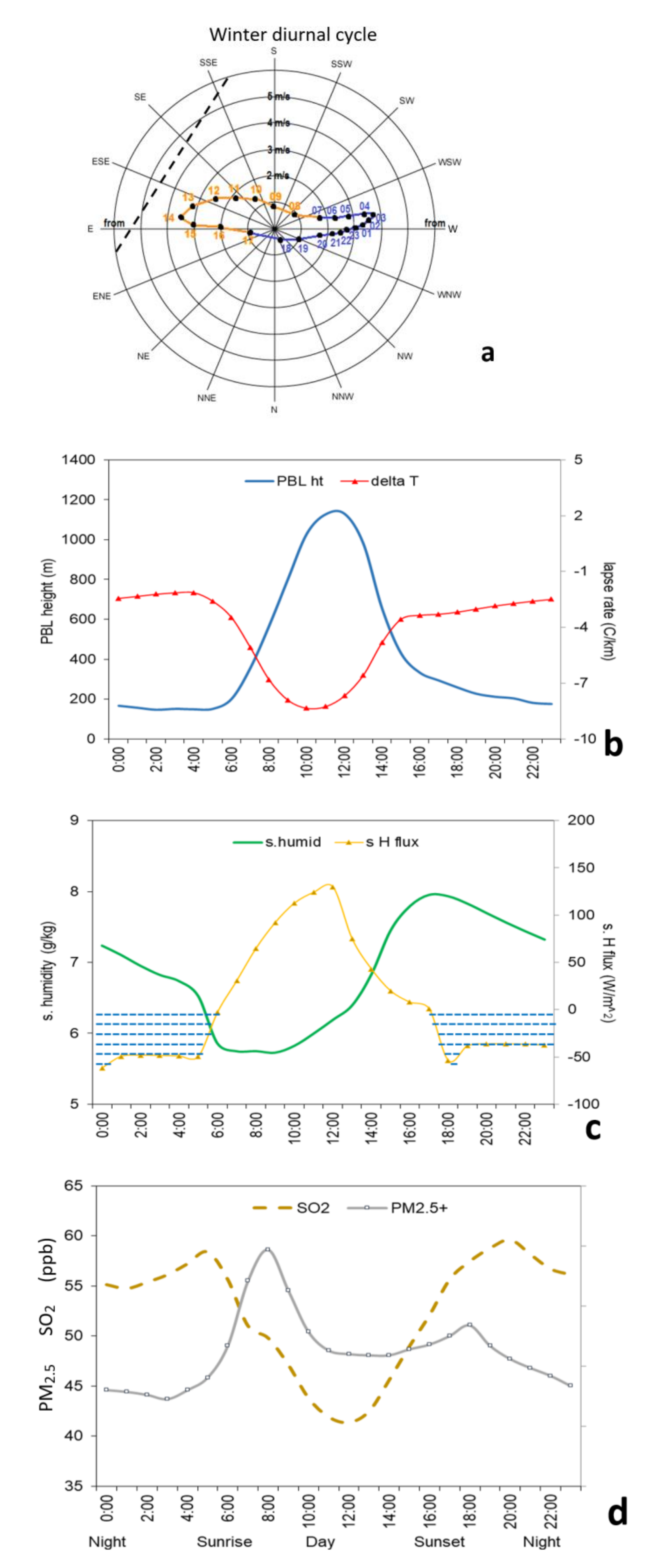
The winter mean diurnal cycle averaged over the Durban-area is plotted in Figure 6a–d. The hodograph illustrates zonal winds that rotate counterclockwise, as expected for inertial airflow with negative Coriolis effect. Westerly winds ~3 m/s prevail in the early hours, then decrease in speed after sunrise. Winds swing through southeasterly and accelerate by afternoon, then diminish near sunset and rotate back to westerly. Two speed minima follow the morning and evening rush hours, so traffic emissions are less dispersed. The PBL height and delta T follow the solar angle and reach maximum mixing depth (1000 m) and instability (−7 °C/km) around 11:00–12:00 UTC (13:00–14:00 local). At night the mean lapse rate is only −2 °C/km within a PBL height of <200 m.
According to reanalysis, the diurnal cycle is gaussian except for specific humidity and sensible heat flux. There is a drying trend around sunrise following the downslope land breeze, and a moistening trend around sunset following the upslope sea breeze. Sensible heat fluxes are −40 W/m2 at night and rise quickly during the morning to exceed 100 W/m2 by mid-day. Table 5 lists the cross-correlations with SO2 and PM2.5 over the mean diurnal cycle. Durban-area SO2 increases at night (Figure 6d) during land breezes (-V wind) characterized by a stable lapse rate, shallow PBL height (r = −0.95) and negative sensible heat flux. High PM2.5 concentrations follow the morning rush-hour and coincide with the land−sea breeze transition. The afternoon peak of PM2.5 is flattened by sea breezes, yielding asymmetry and weak diurnal correlations.
3.6. Dispersion in Winter
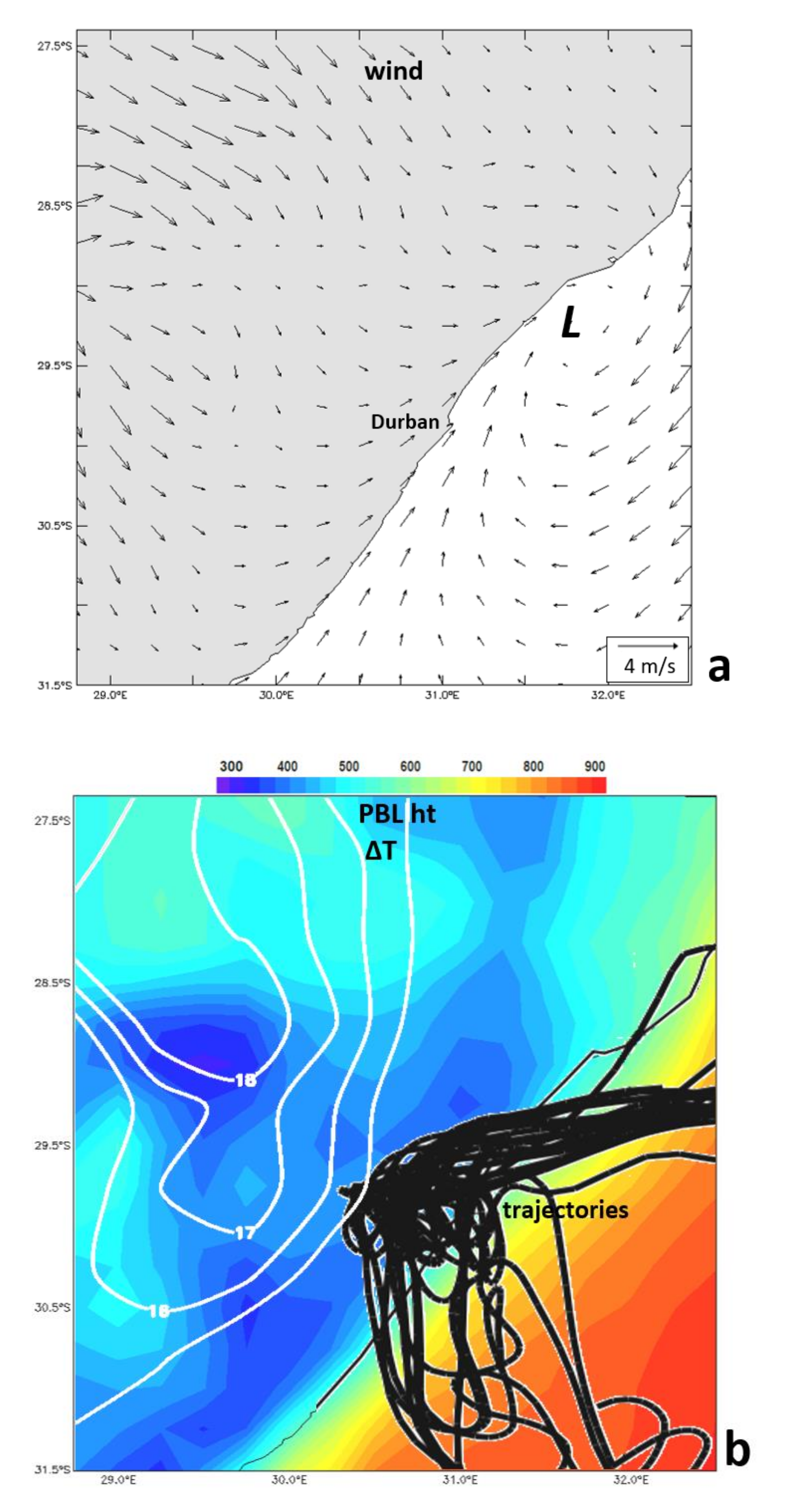
We focus on how the winter weather inhibits dispersion by mesoscale analysis of the July 2015 patterns. Near-surface winds over the interior are northwesterly but tend to split around the Drakensberg and diminish over the Tugela Valley (Figure 7a). Nearshore southwesterlies and offshore northeasterlies suggest a standing coastal low. The PBL was only 350 m deep over the coastal plains in July 2015 (Figure 7b). Twice-daily HYSPLIT emission trajectories tend to loop and recirculate before heading southeastward in the prevailing airflow. The diurnal temperature range that induces land−sea breezes exceeds 15 °C just west of Durban.
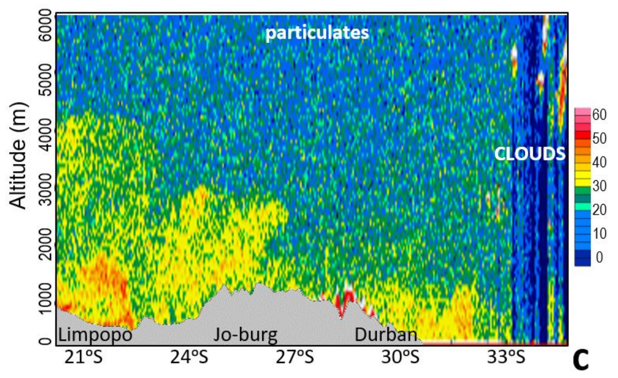
A CALIPSO vertical section on 12 July 2015 (Figure 7c) reveals a 2 km layer of high-density particulates above the surface: a mixture of continental dust and emissions from urban, industrial and agricultural sources. Supplementary Figure S2a suggests that HYSPLIT-simulated plumes from Highveld industries (near Johannesburg) reach Durban after 36 h of prefrontal weather.
3.7. Air Pollution Episode 10–24 July 2015
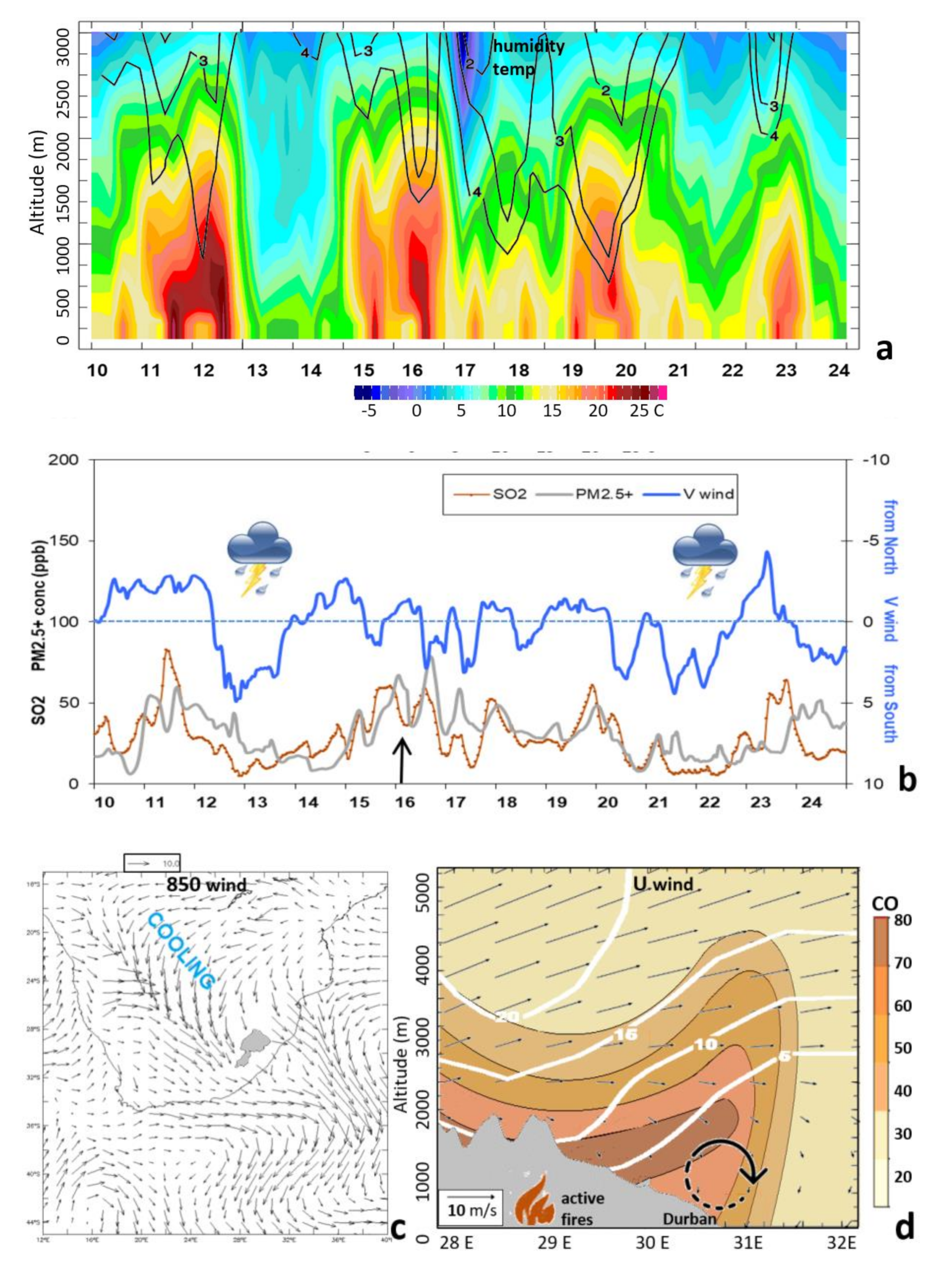
The July 2015 period was characterized by pulses of warm, dry, calm weather on 11–12, 15–16, 19–20 and 23 July 2015 (Figure 8a) that led to SO2 and PM2.5 concentrations > 50 ppb (Figure 8b). The near-surface wind map of 15–16 July 2015 (Figure 8c) illustrates a prefrontal trough with northwesterly winds >10 m/s accompanied by nocturnal cooling < −60 W/m2 across the Kalahari. The stable airflow splits around the Drakensburg and slows over Durban.
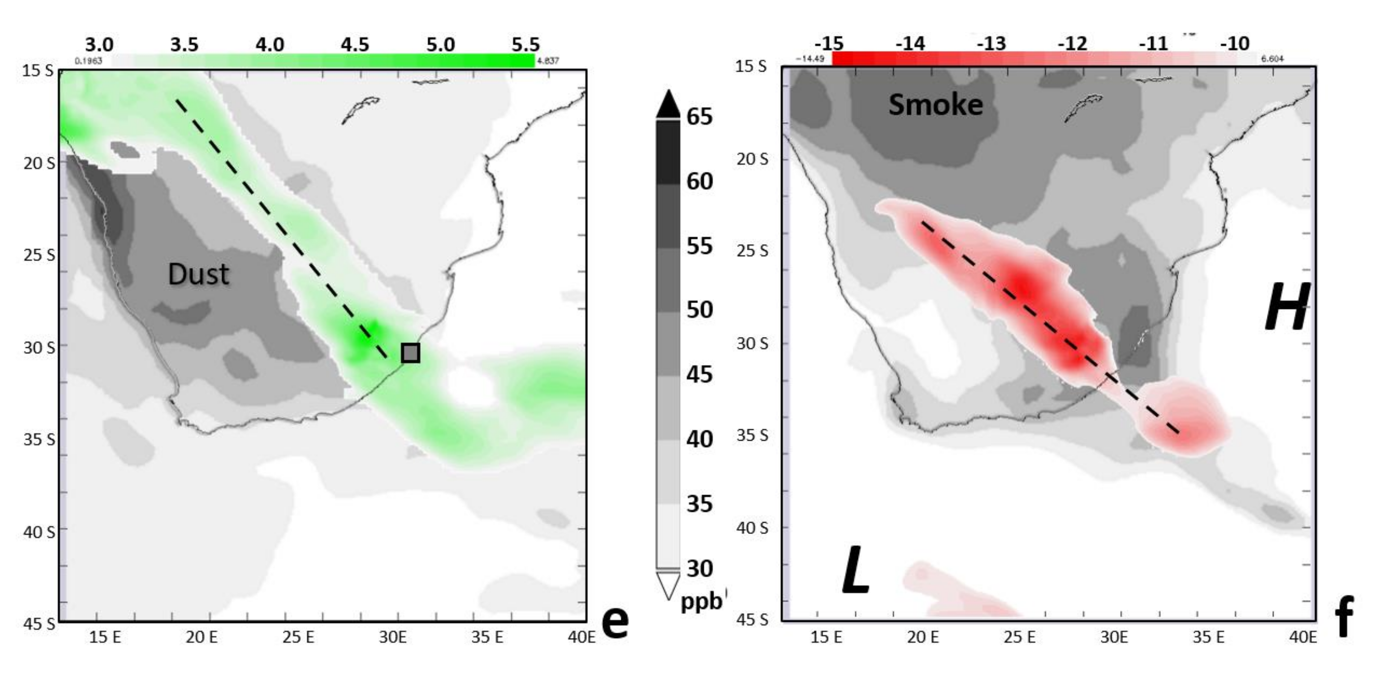
The east−west vertical section of satellite CO and zonal circulation on 15–16 July 2015 (Figure 8d) shows that the westerly airflow is sheared by upstream mountains, inducing a leeward rotor and descending motion over the coastal plains (29.6° E, 850 hPa) that concentrates air pollutants, including particulate-laden agricultural smoke plumes [52]. Radiosonde profiles on 16 July 2015 (Table 6) exhibit a stable lapse rate and subsidence inversion in the layer 950–900 hPa. Dewpoint temperatures decline to −2 °C by 850 hPa, indicative of dry continental air. Radiosonde winds of ~4 m/s alternate from 220–250° at night to 040–090° in the day, indicative of land−sea breezes beneath the berg winds. Regional maps of MERRA2 dust and smoke concentrations on 15–16 July 2015 (Figure 8e,f) reveal plumes drawn toward Durban by a prefrontal trough. These plumes would usually pass westward into the tropical Atlantic [8,53]. Dust emissions from the Kalahari are advected by a westerly airflow behind the trough, while smoke emissions from the Zambezi are advected by a northerly airflow in front of the trough. Although these particulate emissions undergo ~106-fold dispersion during ~106 m of transport to Durban, the blocking Mascarene high and winter nocturnal cooling act to concentrate the plumes.
Hourly cross-correlations in the 10–24 July 2015 period (Table 7) indicate that in situ PM2.5 follows SO2 [54]. Both pollutants are significantly correlated with ERA5 temperature and delta T (r = 0.51 to 0.66) and negatively correlated with humidity and SLP (r = −0.43 to −0.73). Negative cross-correlations amongst the meteorological variables are significant for delta T and PBL height and for SLP and temperature—owing to coastal lows accompanying westerly troughs [51].
3.8. Predictive Potential
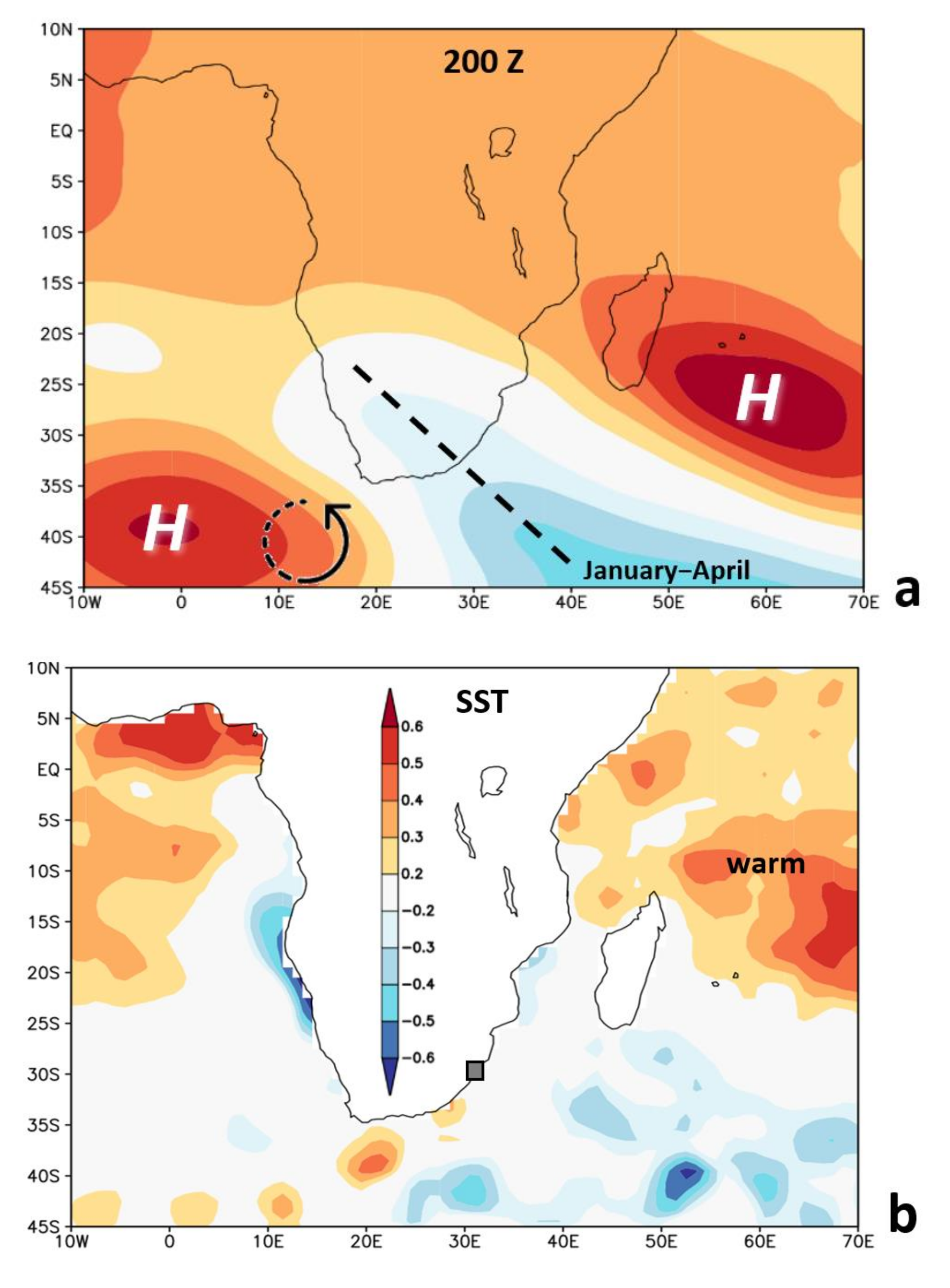
The earlier finding that WIO SST is correlated with the Durban API during winter (cf. Figure 3d) led us to consider its predictive potential and links to local weather. Point-to-field regression maps for the preceding January–April season reveal a peculiar 200 hPa geopotential height pattern (Figure 9a). Positive values spread across tropical Africa before winters with high air pollution in Durban. An NW-tilted upper trough is seen over South Africa in January–April that migrates toward Madagascar by May–August. Paired with the trough is an upper ridge in the South Atlantic that imparts an anticyclonic curvature to the jet stream. This feature migrates over Durban during winter, increasing the probability of dry prefrontal weather and blocking by the Mascarene high.
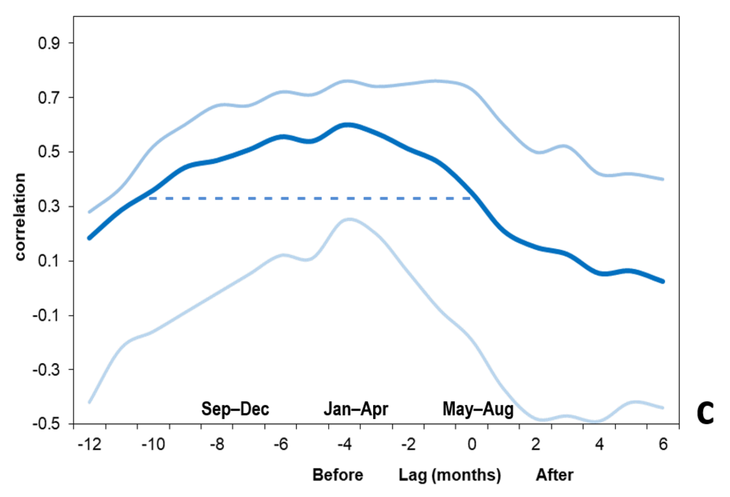
The SST point-to-field correlation map (Figure 9b) indicates a large warm area over the WIO (20°–10° N, 40°–85° E) in the preceding January–April season. This feature is characteristic of the Indian Ocean Dipole [55,56] and the deepening of the thermocline. We also note a warm signal in the Gulf of Guinea and cooler SST in the mid-latitudes off Durban. Lead/lag correlations of the Durban May−August API with WIO SST (Figure 9c) reveal a steady association (r > 0.4 from −9 to 0 months). Our long-range predictive index links the “see-saw” of the tropical Indian Ocean to atmospheric dispersion over Durban via troughs in the subtropical jet stream.
Short-term warnings of winter air pollution would use pattern recognition: “matching” the 500 hPa anomaly maps (Figure 4c,d) and near-surface prefrontal winds (Figure 5a) with operational forecasts. Temporal cross-correlations determined that near-surface dewpoint temperature coincides with light northwesterly airflow (r = –0.49) and thermally stable conditions that constitute poor atmospheric dispersion (Table 3: NO2, O3). Hence near-surface humidity or dewpoint temperature forecasts become a useful tool for anticipating the harmful impacts of air pollution.
4. Discussion
This study has increased our understanding of environmental conditions governing the dispersion of trace gases and particulates over Durban, South Africa, using modern air chemistry and meteorology reanalysis of satellite and in situ measurements underpinned by a dense network of observations (Figures S2b and S3c). Surface concentrations of trace gases peak in May–June–July while particulates extend into August–September [57], contributing to respiratory mortality. The mean maps of CO and NO2 show the highest concentrations ~10 km inland from Durban. Local point-to-field regression maps (Figure 3e–g) indicate a trough extending to the warm Agulhas Current inducing a northwesterly airflow over the Drakensberg. This weather scenario induces a leeward rotor within the stable descending motion over the coastal plains during winter air pollution events (Figure 5c). While dry prefrontal weather during winter accumulates trace gases and particulates, a similar pattern during summer (November–April) often leads to rainfall, wet deposition and clean air.
We formulated monthly and daily API time series as the sum of trace gases and particulates (CO + NO2 + O3 + PM2.5 + SO2) assimilated from satellite and in situ measurements since 2001. Pair-wise cross-correlations affirmed that dry northwesterly airflow, stable lapse rates and shallow mixing depths accumulate air pollutants in the coastal valleys. Multivariate regression of the daily API onto 14 weather variables determined that 1000–850 hPa zonal wind and delta temperature were influential. Daily histograms (Figure 2e,f) revealed that poor dispersion occurs ~25% of the time during winter. HYSPLIT-simulated trajectories (Figure 7b) often join the marine airflow (Figure 2a) that is pulsed by transient low- and high-pressure cells. The inland decrease of wind speed and mixing depth (Figure 2a,c) caused by surface roughness >1 m in the Valley of a Thousand Hills (Figure S3a,b) suggests that new emissions should be pushed coastward to achieve better dispersion. However, such a mitigating strategy may conflict with aesthetic value, tourism and prior urbanization.
The mean diurnal cycle shows a lull in winds following morning and afternoon rush hour and east−west oscillations that recirculate pollutants (Figure 6a). The “thermal” axis differs from coastal orientation. The equation U = (g h)/T (∂T/∂x) ∂t [58] can be used to understand this effect: with temperature T ~285 K, depth of cooling h ~25 m, nocturnal gradient ∂T/∂x ~10−4 K/m and duration ∂t ~4 × 10⁴ s. The outcome is land−sea breezes ~3 m/s that rotate counter-clockwise beneath a thermal inversion (Table 6). Surface winds ~7 m/s on the coast are channelized 040°/200° by the synoptic weather, whereas inland (Figure S3b) the airflow is sluggish and diurnal. A warmer Agulhas Current (Figure 3f) enhances the thermal gradient supporting land breezes.
Point-to-field regression maps of the winter API onto regional SST found warming in the tropical WIO at ~6 month lead time (Figure 9b,c). The correlation map formed an upper level atmospheric Rossby wave-train (Figure 9a) that underpins prefrontal weather. The top-10 daily composite pattern involved a deep trough over the Northern Cape and a blocking Mascarene high. The slow eastward progression of this low–west/high–east pattern redirects particulate-laden Kalahari dust and Zambezi smoke plumes toward Durban.
We note that the tropical Indian Ocean experiences 3 to 5 yr undulations of the thermocline (see-saw) forming an east−west Dipole [56]. As warm seawater nears East Africa [59], atmospheric convection over the WIO alters the upper circulation as seen in Figure 9a [60]. This suppresses rainfall over southern Africa during summer and leads to more PM2.5 dust aerosols reaching Durban in the following winter.
Our findings suggest that air pollution warnings could be issued with: (i) dewpoint temperature < 5 °C under light northwesterly airflow, (ii) trough over the Northern Cape during winter and (iii) following a dry summer with warm WIO SST.
Further work will include satellite/reanalysis validation with in situ data, understanding links between sensible heat flux and PBL height, and meso-scale analysis of eddies forming leeward of the escarpment under dry northwesterly airflow. We anticipate that urban hot spots will emerge with greater confidence from data assimilation at 10 km horizontal resolution.
Supplementary Materials
The following supporting information can be downloaded at https://0-www-mdpi-com.brum.beds.ac.uk/article/10.3390/atmos13050811/s1: Figure S1: (a) Aerial photo of Durban looking southeastward above the intersection of N-2 and N-3 highways. Reprinted from ref. [61] (b) Wavelet analysis of inter-annual filtered Durban-area API: reflecting ~2.5 and 5 yr cycles within the cone of validity. Spectral energy shaded from 90 to 99% confidence. Figure S2. (a) Plume arrival time in hours during a top-10 day of Durban-area API, based on a HYSPLIT dispersion simulation of virtual emissions from the Highveld near Johannesburg (30–31 July 2009). Prefrontal weather of >36 h duration brings air pollution from the interior. Objectively analyzed 850 hPa wind streamlines are superimposed and min/max speeds are labelled. (b) Long-term mean surface reporting frequency: grey-shaded 3rd order stations & ships, blue squares 2nd order stations (#/month) from SAWS, star is the station used for dewpoint validation (Figure S3c). Figure S3. (a) Surface roughness parameterization at 25 km resolution over KZN. (b) Scatterplot of daily ERA5 surface wind speed & direction: inland 29.6° S, 30.4° E vs. coast 29.9° S, 31° E (2005–2020) at I & C on map (N = 5840). (c) Comparison of 10–24 July 2015 hourly dewpoint temperature station vs. ERA5 reanalysis with linear fit at ![Atmosphere 13 00811 i001]() > on map (N = 360).
> on map (N = 360).
 > on map (N = 360).
Author Contributions
Conceptualization: M.S.B.; Writing – original draft: M.R.J.; Writing – review & editing: M.R.J. All authors have read and agreed to the published version of the manuscript.
Funding
The APC was funded by the South Africa Dept. of Education via the University of Zululand.
Informed Consent Statement
Not applicable.
Data Availability Statement
A 30+ Mb spreadsheet is available on request to the corresponding author.
Acknowledgments
Much of the air constituents and meteorology data were drawn from the following websites: NASA-Giovanni, KNMI Climate Explorer, IRI Climate Library, APDRC-Hawaii, NOAA Ready-ARL and University of Wyoming Radiosonde.
Conflicts of Interest
The authors declare no conflict of interest.
References
- Akimoto, H. Global Air Quality and Pollution. Science 2003, 302, 1716–1719. [Google Scholar] [CrossRef] [PubMed] [Green Version]
- Scorgie, Y. Urban Air Quality Management and Planning in South Africa. Ph.D. Thesis, University of Johannesburg, Johannesburg, South Africa, 2012; p. 333. [Google Scholar]
- Jury, M.R. Statistics and Meteorology of Air Pollution Episodes over the South African Highveld Based on Satellite–Model Datasets. J. Appl. Meteorol. Clim. 2017, 56, 1583–1594. [Google Scholar] [CrossRef]
- Tularam, H.; Ramsay, L.F.; Muttoo, S.; Brunekreef, B.; Meliefste, K.; De Hoogh, K.; Naidoo, R.N. A hybrid air pollution/land use regression model for predicting air pollution concentrations in Durban, South Africa. Environ. Pollut. 2021, 274, 116513. [Google Scholar] [CrossRef] [PubMed]
- Jury, M.R.; Freiman, T. The climate of tropical southern Africa during the Safari 2000 campaign. S. Afr. J. Sci. 2002, 98, 527–533. [Google Scholar]
- Silva, J.M.N.; Pereira, J.M.C.; Cabral, A.I.; Sá, A.C.L.; Vasconcelos, M.J.P.; Mota, B.; Grégoire, J. An estimate of the area burned in southern Africa during the 2000 dry season using SPOT-VEGETATION satellite data. J. Geophys. Res. Earth Surf. 2003, 108. [Google Scholar] [CrossRef] [Green Version]
- Ma, X.; Bartlett, K.; Harmon, K.; Yu, F. Comparison of AOD between CALIPSO and MODIS: Significant differences over major dust and biomass burning regions. Atmos. Meas. Tech. 2013, 6, 2391–2401. [Google Scholar] [CrossRef] [Green Version]
- Bhattachan, A.; D’Odorico, P.; Baddock, M.; Zobeck, T.M.; Okin, G.; Cassar, N. The Southern Kalahari: A potential new dust source in the Southern Hemisphere? Environ. Res. Lett. 2012, 7, 024001. [Google Scholar] [CrossRef] [Green Version]
- Thambiran, T.; Diab, R. Air pollution and climate change co-benefit opportunities in the road transportation sector in Durban, South Africa. Atmos. Environ. 2011, 45, 2683–2689. [Google Scholar] [CrossRef]
- Friedrich, E.; Gopaul, A.; Stretch, D. Public Transportation and Greenhouse Gas Emissions: A Case Study of the e Thekwini Municipality, South Africa. Curr. Trends Civ. Struct. Eng. 2019, 3. [Google Scholar] [CrossRef]
- Preston-Whyte, R.A.; Diab, R.D. Local weather and air pollution potential: The case of Durban. Environ. Conserv. 1980, 7, 241–244. [Google Scholar] [CrossRef]
- Preston-Whyte, R.A.; Tyson, P.D. Atmosphere and Weather of Southern Africa; Oxford University Press: Oxford, UK, 1988; p. 374. [Google Scholar]
- Diab, R.D.; Scott, D. Urban Air Pollution and Quality of Life: Case Study of Durban South Africa. In Proceedings of the 19th Annual Meeting of the International Association for Impact Assessment, Glasgow, UK, 15–19 June 1999. [Google Scholar]
- Matooane, L.; Diab, R.D. Air pollution carrying capacity in the South Durban Industrial Basin. S. Afr. J. Sci. 2001, 97, 450–453. [Google Scholar]
- Diab, R.; Matooane, M. Health risk assessment for sulphur dioxide pollution in south Durban South Africa. Arch. Environ. Health 2003, 58, 763–770. [Google Scholar]
- Ramsay, L.F. Power and Perception : A Political Ecology of Air Pollution in [Durban] South Africa. Ph.D. Thesis, University of Cambridge, Cambridge, UK, 2010; p. 373. [Google Scholar]
- Diab, R.D.; Prause, A.; Bencherif, H. Analysis of SO2 pollution in the south Durban industrial basin. S. Afr. J. Sci. 2002, 98, 543–546. [Google Scholar]
- Simpson, A.J.; McGee, O.S. Air pollution over Pietermaritzburg during the passage of cold fronts. S. Afr. J. Sci. 1996, 92, 45–46. [Google Scholar]
- Simpson, A.J.; McGee, O.S. Analysis of the fumigation effect on pollutants over Pietermaritzburg. S. Afr. Geogr. J. 1996, 78, 41–46. [Google Scholar] [CrossRef]
- Burrows, J.P.; Platt, U.; Borrell, P. (Eds.) The Remote Sensing of Tropospheric Composition from Space; Springer: Berlin, Germany, 2011; p. 536. [Google Scholar]
- Krotkov, N.A.; McLinden, C.A.; Li, C.; Lamsal, L.N.; Celarier, E.A.; Marchenko, S.V.; Swartz, W.H.; Bucsela, E.J.; Joiner, J.; Duncan, B.N.; et al. Aura OMI observations of regional SO2 and NO2 pollution changes from 2005 to 2015. Atmos. Chem. Phys. 2016, 16, 4605–4629. [Google Scholar] [CrossRef] [Green Version]
- Sundström, A.-M.; Nikandrova, A.; Atlaskina, K.; Nieminen, T.; Vakkari, V.; Laakso, L.; Beukes, J.P.; Arola, A.; Van Zyl, P.G.; Josipovic, M.; et al. Characterization of satellite-based proxies for estimating nucleation mode particles over South Africa. Atmos. Chem. Phys. 2015, 15, 4983–4996. [Google Scholar] [CrossRef] [Green Version]
- Korhonen, K.; Giannakaki, E.; Mielonen, T.; Pfüller, A.; Laakso, L.; Vakkari, V.; Baars, H.; Engelmann, R.; Beukes, J.P.; Van Zyl, P.G.; et al. Atmospheric boundary layer top height in South Africa: Measurements with lidar and radiosonde compared to three atmospheric models. Atmos. Chem. Phys. 2014, 14, 4263–4278. [Google Scholar] [CrossRef] [Green Version]
- Ukhov, A.; Mostamandi, S.; Krotkov, N.; Flemming, J.; Da Silva, A.; Li, C.; Fioletov, V.; McLinden, C.; Anisimov, A.; Alshehri, Y.M.; et al. Study of SO2 Pollution in the Middle East Using MERRA-2, CAMS Data Assimilation Products, and High-Resolution WRF-Chem Simulations. J. Geophys. Res. Atmos. 2020, 125, e2019JD031993. [Google Scholar] [CrossRef]
- Molod, A.; Takacs, L.; Suarez, M.; Bacmeister, J. Development of the GEOS-5 atmospheric general circulation model: Evolution from MERRA to MERRA2. Geosci. Model Dev. 2015, 8, 1339–1356. [Google Scholar] [CrossRef] [Green Version]
- GEOS-5 Data Assimilation System. 2016. Available online: http://gmao.gsfc.nasa.gov/pubs/docs/GEOS-5.0.1_Documentation_r3.pdf (accessed on 20 June 2021).
- Wells, R.B.; Lloyd, S.M.; Turner, C.R. National Air Pollution Source Inventory. Air Pollution and its Impacts on the South African Highveld; Held, G., et al., Eds.; Environmental Scientific Association: Pretoria, South Africa, 1996; pp. 3–9. [Google Scholar]
- World Health Organization. WHO Global Ambient Air Pollution Database. 2021. Available online: www.who.int/data/gho/data/themes/air-pollution/who-air-quality-database# (accessed on 20 June 2021).
- World Bank Data. Statistical Database. 2021. Available online: https://data.worldbank.org/indicator/%20EN.ATM.CO2E.KT?%20locations=ZA (accessed on 20 June 2021).
- Josipovic, M.; Annegarn, H.J.; Kneen, M.A.; Pienaar, J.J.; Piketh, S.J. Atmospheric dry and wet deposition of sulphur and nitrogen species and assessment of critical loads of acidic deposition exceedance in South Africa. S. Afr. J. Sci. 2011, 107, 1–10. [Google Scholar] [CrossRef]
- Conradie, E.; Van Zyl, P.; Pienaar, J.; Beukes, J.; Galy-Lacaux, C.; Venter, A.; Mkhatshwa, G. The chemical composition and fluxes of atmospheric wet deposition at four sites in South Africa. Atmos. Environ. 2016, 146, 113–131. [Google Scholar] [CrossRef] [Green Version]
- eThekwini. Greenhouse Gas Emissions Inventory. 2019. Available online: www.durban.gov.za/City_Services/energyoffice (accessed on 20 June 2021).
- Randles, C.A.; Da Silva, A.M.; Buchard, V.; Colarco, P.R.; Darmenov, A.; Govindaraju, R.; Smirnov, A.; Holben, B.; Ferrare, R.; Hair, J.; et al. The MERRA-2 Aerosol Reanalysis, 1980 Onward. Part I: System Description and Data Assimilation Evaluation. J. Clim. 2017, 30, 6823–6850. [Google Scholar] [CrossRef]
- Bucsela, E.J.; Krotkov, N.A.; Celarier, E.A.; Lamsal, L.N.; Swartz, W.H.; Bhartia, P.K.; Boersma, K.F.; Veefkind, J.P.; Gleason, J.F.; Pickering, K.E. A new stratospheric and tropospheric NO2 retrieval algorithm for nadir-viewing satellite instruments, applications to OMI. Atmos. Meas. Tech. 2013, 6, 2607–2626. [Google Scholar] [CrossRef] [Green Version]
- Levy, R.C.; Mattoo, S.; Munchak, L.A.; Remer, L.A.; Sayer, A.M.; Patadia, F.; Hsu, N.C. The Collection 6 MODIS aerosol products over land and ocean. Atmos. Meas. Tech. 2013, 6, 2989–3034. [Google Scholar] [CrossRef] [Green Version]
- Lamsal, L.N.; Krotkov, N.A.; Celarier, E.A.; Swartz, W.H.; Pickering, K.E.; Bucsela, E.J.; Gleason, J.F.; Martin, R.V.; Philip, S.; Irie, H.; et al. Evaluation of OMI operational standard NO2 column retrievals using in situ and surface-based NO2 observations. Atmos. Chem. Phys. 2014, 14, 11587–11609. [Google Scholar] [CrossRef] [Green Version]
- DAQM. Durban Air Constituents. 2021. Available online: http://aqicn.org/city/Durban (accessed on 20 June 2021).
- Saha, S.; Moorthi, S.; Wu, X.; Wang, J.; Nadiga, S.; Tripp, P.; Behringer, D.; Hou, Y.-T.; Chuang, H.-Y.; Iredell, M.; et al. The NCEP Climate Forecast System Version 2. J. Clim. 2014, 27, 2185–2208. [Google Scholar] [CrossRef]
- Hersbach, H.; Bell, B.; Berrisford, P.; Hirahara, S.; Horanyi, A.; Muñoz-Sabater, J.; Nicolas, J.; Peubey, C.; Radu, R.; Schepers, D.; et al. The ERA5 global reanalysis. Q. J. R. Meteorol. Soc. 2020, 146, 1999–2049. [Google Scholar] [CrossRef]
- Gelaro, R.; McCarty, W.; Suárez, M.J.; Todling, R.; Molod, A.; Takacs, L.; Randles, C.A.; Darmenov, A.; Bosilovich, M.G.; Reichle, R.; et al. The modern-era retrospective analysis for research and applications, v2 (MERRA-2). J. Clim. 2017, 30, 5419–5454. [Google Scholar] [CrossRef]
- World Meteorological Organization. WMO Satellite Air Chemistry; World Meteorological Organization: Geneva, Switzerland, 2021. [Google Scholar]
- South Africa Department of Health. Monthly Provincial Respiratory Mortality Data; South Africa Department of Health: Pretoria, South Africa, 2021. [Google Scholar]
- Stein, A.F.; Draxler, R.R.; Rolph, G.D.; Stunder, B.J.B.; Cohen, M.D.; Ngan, F. NOAA HYSPLIT atmospheric transport and dispersion modelling system, Bull. Amer. Meteorol. Soc. 2015, 96, 2059–2077. [Google Scholar] [CrossRef]
- Winker, D.M.; Hunt, W.H.; McGill, M.J. Initial performance assessment of CALIOP. Geophys. Res. Lett. 2007, 34, L19803. [Google Scholar] [CrossRef] [Green Version]
- Shikwambana, L.D.; Sivakumar, V. Investigation of various aerosols over different locations in South Africa using satellite, model simulations and LIDAR. Meteorol. Appl. 2019, 26, 275–287. [Google Scholar] [CrossRef] [Green Version]
- IEM. Iowa Environmental Mesonet, Wind Rose Analysis from Durban Airport. 2021. Available online: http://mesonet.agron.iastate.edu/sites/windrose.phtml?station=FALE&network=ZA__ASOS (accessed on 20 June 2021).
- Piketh, S.J.; Annegarn, H.J.; Tyson, P.D. Lower tropospheric aerosol loadings over South Africa: The relative contribution of aerosol dust, industrial emissions, and biomass burning. J. Geophys. Res. 1999, 104, 1597–1607. [Google Scholar] [CrossRef]
- Hersey, S.P.; Garland, R.M.; Crosbie, E.; Shingler, T.; Sorooshian, A.; Piketh, S.J.; Burger, R. An overview of regional and local characteristics of aerosols in South Africa using satellite, ground, and modeling data. Atmos. Chem. Phys. 2015, 15, 4259–4278. [Google Scholar] [CrossRef] [Green Version]
- Zubkova, M.; Boschetti, L.; Abatzoglou, J.T.; Giglio, L. Changes in Fire Activity in Africa from 2002 to 2016 and Their Potential Drivers. Geophys. Res. Lett. 2019, 46, 7643–7653. [Google Scholar] [CrossRef] [Green Version]
- FIRMS. Fire Information Resource Management System. 2021. Available online: https://firms.modaps.eosdis.nasa.gov/ (accessed on 20 June 2021).
- Scott, G.M.; Diab, R. Forecasting Air Pollution Potential: A Synoptic Climatological Approach. J. Air Waste Manag. Assoc. 2000, 50, 1831–1842. [Google Scholar] [CrossRef]
- GSFC 2021: Satellite Monitored Fires. Available online: https://svs.gsfc.nasa.gov/14108 (accessed on 20 June 2021).
- Jury, M.R.; Whitehall, K. Warming of an elevated layer over Africa. Clim. Chang. 2009, 99, 229–245. [Google Scholar] [CrossRef]
- Zunckel, M.; Robertson, L.; Tyson, P.; Rodhe, H. Modelled transport and deposition of sulphur over Southern Africa. Atmos. Environ. 2000, 34, 2797–2808. [Google Scholar] [CrossRef]
- Yamagata, T.; Behera, S.K.; Luo, J.-J.; Masson, S.; Jury, M.R.; Rao, S.A. Coupled Ocean-Atmosphere Variability in the Tropical Indian Ocean, in Earth Climate: The Ocean-Atmosphere Interaction; Wang, C., Xie, S.P., Carton, J.A., Eds.; American Geophysical Union: Washington, DC, USA, 2003; pp. 189–212. [Google Scholar]
- Jury, M.R.; Huang, B. The Rossby wave as a key mechanism of Indian Ocean climate variability. Deep Sea Res. 2004, 51, 2123–2136. [Google Scholar] [CrossRef]
- Shikwambana, L.D. Lidar and Satellite Observation of Aerosols and Clouds over South Africa. Ph.D. Thesis, University of KwaZulu-Natal, Durban, South Africa, 2017; p. 158. Available online: https://ukzn-dspace.ukzn.ac.za/ (accessed on 20 June 2021).
- Pielke, R.A.; Segal, M. Mesoscale Circulations Forced by Differential Terrain Heating. In Mesoscale Meteorology & Forecasting; Ray, P.S., Ed.; American Meteorological Society: Boston, MA, USA, 1986; pp. 516–548. [Google Scholar]
- Nagura, M.; McPhaden, M.J. Dynamics of zonal current variations associated with the Indian Ocean dipole. J. Geophys. Res. Earth Surf. 2010, 115, C11026. [Google Scholar] [CrossRef]
- Jury, M.R. South Indian Ocean Rossby Waves. Atmosphere-Ocean 2018, 56, 322–331. [Google Scholar] [CrossRef]
- De Wet, A. N3 Freeway on its final approach into Durban, Spaghetti Junction (N3-N2) in foreground 2011. Available online: https://commons.wikimedia.org/wiki/File:DurbanN3-aerial.jpg (accessed on 20 June 2021).
Figure 1.
Maps of (a) elevation and urbanization (grey) and (b) satellite nocturnal land surface temperature and SST isotherms (°C) with airport icons and in-situ stations (+). Long-term mean surface maps of (c) MERRA2 CO, (d) OMI NO2 concentration (ppb), with elevations, major rivers and local maximum (x). Temporal graphs of (e) monthly Durban-area surface API, and (f) its mean annual cycle and upper/lower terciles (summed concentration Σ ppb). “Durban-area” is the dashed box in (a), dashed line is the section; KZN mean respiratory mortality bar chart in (f) uses right axis (#/month).

Figure 2.
Climatology of atmospheric dispersion via May–August mean longitude slices on 29.8° S for ERA5: (a) surface wind speed, (b) sensible heat flux and (c) PBL height. (d) Mean annual cycle of ERA5 dewpoint temperature. Histograms of Durban-area winter season: (e,f) ERA5 near-surface wind speed and direction. In (a–c) the longitude of Durban is given (upper).

Figure 3.
Point-to-field correlations (2001–2020) with respect to May–August monthly API for: (a) ERA5 sea level air pressure (SLP) with lows and place names, (b) ERA5 200 hPa geopotential height with high, (c) satellite net outgoing longwave radiation (OLR) and (d) sea surface temp (SST). Point-to-field regressions (N = 20) with May–August API for local: (e) SLP with icons, (f) surface air temperature, and (g) surface zonal wind with vectors; illustrating winter patterns associated with high air pollution over Durban; upper panels use the correlation scale at right; lower row has individual scales. Zambezi and Kalahari shown in (a); satellite July–September mean fire density grey-shaded in (d); dashed line in (e) refers to coastal trough; vectors in (f) highlight the Agulhas Current.

Figure 4.
(a) Time series of daily cumulative API over Durban (Σ ppb). Point-to-field correlations (May–August 2005–2020) with respect to daily API for ERA5 sea-level pressure (SLP): (b) −3, (c) −2, (d) −1 days before high air pollution in Durban (N = 1920). Composite anomalies of the top-10 air pollution days: (e) 500 hPa geopotential height and (f) winds illustrating a Kalahari trough and Mascarene high (arrows refer to movement from day –1 to day +1).

Figure 5.
Composite maps of top-10 air pollution days listed in Table 4: (a) MERRA2 near-surface winds (m/s) with active fire icon and Durban-area: square, (b) surface ozone and air temperature anomalies > 1.5 C (contour). Composite east−west vertical section on 29.8° S (line in (b)) of top-10 air pollution days: (c) zonal wind (shaded) & circulation (vectors), and (d) specific humidity (g/kg) and meridional wind (dashed contours) with topographic profile, where -V refers to airflow out of the page. Vertical motion in (c) is exaggerated 10-fold.

Figure 6.
Winter mean diurnal cycle of over the Durban-area (2011–2015): (a) hodograph of MERRA2 near-surface wind velocity, all times UTC (local +2) with day-night shading, (b) PBL height and delta temperature, (c) specific humidity and sensible heat flux (nocturnal cooling <0 dashed), (d) DAQM in situ air constituents. Dashed line in (a) is the coastal orientation.

Figure 7.
Mean July 2015: (a) ERA5 surface winds, (b) PBL height and twice-daily HYSPLIT-simulated emission trajectories from the Durban-area; white contours >15 °C are winter mean in situ Tmax–Tmin values. (c) N–S vertical section on 30.5° E of particulate density on 12 July 2015 (ppb) from CALIPSO satellite lidar 0.532 µm backscatter. Vectors in (a) are at 25 km resolution.


Figure 8.
Case of 10–24 July 2015: (a) time–height air temperatures (shaded C) and specific humidity <4 g/kg (contours), (b) time series of hourly SO2, PM2.5, -V wind, & rain icons. 15–16 July 2015, (c) 850 hPa wind (m/s), nocturnal cooling (blue) and highlands (grey), (d) vertical section on 29.8° S of CO (shaded ppb) and zonal circulation (vectors) with white speed contours and leeward eddy, (e) grey-shaded dust (PM2.5) and green-shaded 700 hPa humidity > 3 g/kg, and (f) grey-shaded smoke and red-shaded 700 hPa V wind <−10 m/s.


Figure 9.
Point-to-field correlation of May−August air pollution index (cf. Figure 1e) with prior Jan−Apr: (a) ERA5 200 hPa geopotential height, anticyclonic spin behind dashed trough, (b) SST (at −4 months) illustrating a warmer WIO leads higher pollution. (c) Lead/lag correlation of May−August air pollution index with WIO SST and terciles 2001–2020 with dashed 90% confidence threshold. Correlation color-bar for maps is given in (b), Durban is the grey square.


Table 1.
Datasets used in the analysis [41].
Table 1.
Datasets used in the analysis [41].
| Acronym | Name | Space, Time Resolution | Quantity |
|---|---|---|---|
| AIRS * | Atmospheric Infrared Sounder | 100 km, twice daily | Near-surface CO concentration |
| CALIPSO | Cloud-Aerosol Lidar & Infrared Pathfinder Satellite Observation | ~1 km on N-S slice, weekly | Particulate density |
| CFSr2 | Coupled Forecast System reanalysis version 2 | ~25 km, hour to month | Near-surface meteorology |
| DAQM | Durban air quality monitoring network | Station, hourly intermittent | Surface PM2.5, SO2 |
| ERA5 | European Community reanalysis version 5 | ~25 km, hour to month | Near-surface meteorology |
| HYSPLIT | Hybrid Single Particle Lagrangian Integrated Trajectory Model | ~10 km, along track | Emission transport & dispersion |
| MERRA2 | NASA Meteorology reanalysis version 2 with GEOS-5 air chemistry | ~50 km, hour to month | Near-surface CO, O3, PM2.5, SO2, meteorology |
| MODIS * | Moderate Imaging Spectrometer | 100 km, twice daily | Aerosol Optical Depth (AOD) column |
| OMI * | Ozone Monitoring Instrument | 25 km, twice daily | Near-surface NO2 concentration |
| SADH | South Africa Dept of Health | KZN prov. monthly | Diagnosed respiratory mortality |
| SAWS | South African Weather Service | Radiosonde, surface obs. | Air & dew temp, wind velocity, SLP |
* polar-orbiting satellite data gaps are filled by running-maximum.
Table 2.
Simultaneous pair-wise cross-correlation of surface air constituents and ERA5 1000–850 hPa meteorology variables over the Durban-area: monthly (2001–2020 N = 230).
Table 2.
Simultaneous pair-wise cross-correlation of surface air constituents and ERA5 1000–850 hPa meteorology variables over the Durban-area: monthly (2001–2020 N = 230).
| Monthly | AOD s | CO | NO2 s | O3 | PM2.5 | SO2 | API |
|---|---|---|---|---|---|---|---|
| CO | 0.21 | ||||||
| NO2 s | 0.04 | 0.65 | |||||
| O3 | −0.27 | 0.30 | 0.43 | ||||
| PM2.5 | −0.18 | 0.27 | 0.30 | 0.21 | |||
| SO2 | −0.23 | 0.65 | 0.71 | 0.65 | 0.37 | ||
| API | 0.05 | 0.87 | 0.89 | 0.48 | 0.45 | 0.83 | |
| U wind | −0.11 | 0.46 | 0.54 | 0.38 | 0.40 | 0.46 | 0.57 |
| V wind | −0.43 | −0.24 | −0.02 | 0.27 | −0.06 | 0.11 | −0.10 |
| Temp | 0.10 | −0.43 | −0.65 | −0.39 | −0.16 | −0.57 | −0.59 |
| Humid | 0.08 | −0.69 | −0.79 | −0.56 | −0.33 | −0.82 | −0.84 |
| H flux | 0.24 | −0.37 | −0.47 | −0.58 | −0.32 | −0.67 | −0.52 |
| PBL ht | 0.17 | −0.47 | −0.51 | −0.58 | −0.31 | −0.78 | −0.60 |
Satellite and in situ data denoted by (s) and (i). Bold values are significant above 90% confidence.
Table 3.
Simultaneous pair-wise cross-correlation of surface air constituents and ERA5 1000–850 hPa meteorology variables over the Durban-area: daily (2005–2020 N = 5840).
Table 3.
Simultaneous pair-wise cross-correlation of surface air constituents and ERA5 1000–850 hPa meteorology variables over the Durban-area: daily (2005–2020 N = 5840).
| Daily | AOD s | CO s | O3 | NO2 s | SO2 | API |
|---|---|---|---|---|---|---|
| CO s | 0.32 | |||||
| O3 | 0.19 | 0.62 | ||||
| NO2 s | 0.20 | 0.14 | 0.30 | |||
| SO2 | 0.06 | 0.15 | 0.04 | 0.11 | ||
| API | 0.53 | 0.57 | 0.59 | 0.82 | 0.14 | |
| T dew | 0.02 | −0.13 | −0.54 | −0.45 | 0.00 | −0.42 |
| Humid | 0.01 | −0.16 | −0.56 | −0.44 | −0.01 | −0.43 |
| U wind * | 0.01 | 0.05 | 0.38 | 0.29 | 0.01 | 0.29 |
| V wind | −0.11 | −0.07 | −0.03 | −0.04 | 0.02 | −0.09 |
| Temp | 0.04 | −0.14 | −0.19 | −0.15 | −0.02 | −0.12 |
| SLP | −0.01 | 0.01 | 0.14 | 0.20 | 0.03 | 0.15 |
| delta T * | 0.14 | 0.21 | 0.14 | 0.02 | −0.02 | 0.18 |
Satellite and in situ data denoted by (s) and (i). Bold values are significant above 90% confidence; * identifies weather variables retained in API multivariate regression.
Table 4.
Top-10 air pollution days based on the daily cumulative API shown in Figure 4a.
Table 4.
Top-10 air pollution days based on the daily cumulative API shown in Figure 4a.
| Top-10 days | Ranked API (Σ ppb) |
|---|---|
| 13 July 2005 | 167 |
| 15 July 2006 | 165 |
| 11 July 2015 | 164 |
| 01 Aug 2009 | 157 |
| 12 July 2012 | 156 |
| 30 May 2015 | 150 |
| 10 Aug 2016 | 149 |
| 11 June 2006 | 140 |
| 24 July 2015 | 139 |
| 15 July 2015 | 138 |
Table 5.
Simultaneous pair-wise cross-correlation of surface air constituents and ERA5 1000–850 hPa meteorology variables over the Durban-area: winter mean diurnal cycle (2011–2015 N = 24).
Table 5.
Simultaneous pair-wise cross-correlation of surface air constituents and ERA5 1000–850 hPa meteorology variables over the Durban-area: winter mean diurnal cycle (2011–2015 N = 24).
| Diurnal | PM2.5 i | SO2 i |
|---|---|---|
| U wind | −0.37 | 0.75 |
| V wind | 0.26 | −0.96 |
| speed | −0.67 | −0.02 |
| Temp | 0.64 | −0.90 |
| Humid | −0.48 | 0.60 |
| delta T | −0.63 | 0.88 |
| H flux | 0.57 | −0.93 |
| PBL ht | 0.41 | −0.95 |
Bold values are significant above 90% confidence.
Table 6.
Durban radiosonde profiles 00:00 & 09:00 UTC 16 July 2015.
| PRES | GPH | T | Td | DIR | SPD |
|---|---|---|---|---|---|
| hPa | m | C | C | deg | m/s |
| Night | |||||
| 1000 | 151 | 15.8 | 10.8 | 220 | 3 |
| 984 | 289 | 17.8 | 13.3 | 239 | 4 |
| 970 | 412 | 18.2 | 7.2 | 255 | 4 |
| 962 | 482 | 17.6 | 7.6 | 265 | 3 |
| 941 | 671 | 17.2 | 7.2 | 290 | 4 |
| 925 | 817 | 17.4 | 8.4 | 310 | 5 |
| 906 | 995 | 20.4 | 6.4 | 317 | 6 |
| 900 | 1052 | 21.6 | 5.6 | 319 | 7 |
| 868 | 1363 | 19.3 | 5.2 | 330 | 8 |
| 850 | 1543 | 18.0 | 5.0 | 340 | 10 |
| Day | |||||
| 1000 | 109 | 22.0 | 17.0 | 090 | 4 |
| 985 | 239 | 19.6 | 15.6 | 065 | 4 |
| 970 | 372 | 22.4 | 9.4 | 039 | 5 |
| 955 | 507 | 23.8 | 5.8 | 013 | 5 |
| 948 | 571 | 23.4 | 6.4 | 001 | 5 |
| 925 | 784 | 24.4 | 4.4 | 320 | 6 |
| 910 | 926 | 23.5 | 3.5 | 325 | 7 |
| 890 | 1119 | 22.2 | 2.2 | 336 | 9 |
| 870 | 1315 | 21.4 | −0.1 | 340 | 12 |
| 850 | 1516 | 20.6 | −2.4 | 350 | 16 |
Table 7.
Simultaneous pair-wise cross-correlation of surface air constituents and ERA5 1000–850 hPa meteorology variables over the Durban-area: hourly case study (10–24 July 2015 N = 360).
Table 7.
Simultaneous pair-wise cross-correlation of surface air constituents and ERA5 1000–850 hPa meteorology variables over the Durban-area: hourly case study (10–24 July 2015 N = 360).
| Hourly | PM2.5 i | SO2 i | PBL ht | U Wind | V Wind | Temp | Humid | SLP | Delta T |
|---|---|---|---|---|---|---|---|---|---|
| SO2 i | 0.51 | ||||||||
| PBL ht | −0.13 | −0.21 | |||||||
| U wind | 0.32 | 0.06 | −0.38 | ||||||
| V wind | −0.09 | −0.53 | 0.33 | −0.12 | |||||
| Temp | 0.61 | 0.65 | −0.16 | 0.15 | −0.40 | ||||
| Humid | −0.49 | −0.43 | 0.08 | −0.26 | 0.29 | −0.40 | |||
| SLP | −0.73 | −0.45 | −0.14 | −0.07 | 0.06 | −0.62 | 0.39 | ||
| delta T | 0.51 | 0.43 | −0.73 | 0.55 | −0.41 | 0.48 | −0.35 | −0.21 | |
| H flux | −0.20 | −0.03 | 0.58 | −0.60 | 0.25 | −0.03 | −0.04 | −0.06 | −0.62 |
Satellite and in situ data denoted by (s) and (i). Bold values are significant above 90% confidence.
Publisher’s Note: MDPI stays neutral with regard to jurisdictional claims in published maps and institutional affiliations. |
© 2022 by the authors. Licensee MDPI, Basel, Switzerland. This article is an open access article distributed under the terms and conditions of the Creative Commons Attribution (CC BY) license (https://creativecommons.org/licenses/by/4.0/).
Share and Cite
MDPI and ACS Style
Jury, M.R.; Buthelezi, M.S. Air Pollution Dispersion over Durban, South Africa. Atmosphere 2022, 13, 811. https://0-doi-org.brum.beds.ac.uk/10.3390/atmos13050811
AMA Style
Jury MR, Buthelezi MS. Air Pollution Dispersion over Durban, South Africa. Atmosphere. 2022; 13(5):811. https://0-doi-org.brum.beds.ac.uk/10.3390/atmos13050811
Chicago/Turabian StyleJury, Mark R., and Mandisa S. Buthelezi. 2022. "Air Pollution Dispersion over Durban, South Africa" Atmosphere 13, no. 5: 811. https://0-doi-org.brum.beds.ac.uk/10.3390/atmos13050811
Note that from the first issue of 2016, this journal uses article numbers instead of page numbers. See further details here.