Article

Study on the Water and Heat Fluxes of a Very Humid Forest Ecosystem and Their Relationship with Environmental Factors in Jinyun Mountain, Chongqing

Three-Gorges Reservoir Area (Chongqing) Forest Ecosystem Research Station, School of Soil and Water Conservation, Beijing Forestry University, Beijing 100083, China
*
Author to whom correspondence should be addressed.
Submission received: 9 March 2022 / Revised: 13 May 2022 / Accepted: 17 May 2022 / Published: 19 May 2022
(This article belongs to the Topic Climate Change and Environmental Sustainability)

Abstract

:
The high-humidity mountain forest ecosystem (HHMF) of Jinyun Mountain in Chongqing is a fragile ecosystem that is sensitive to climate change and human activities. Because it is shrouded in fog year-round, illumination in the area is seriously insufficient. However, the flux (energy, water) exchanges (FEs) in this ecosystem and their influencing factors are not clear. Using one-year data from flux towers with a double-layer (25 m and 35 m) eddy covariance (EC) observation system, we proved the applicability of the EC method on rough underlying surfaces, quantified the FEs of HHMFs, and found that part of the fog might also be observed by the EC method. The observation time was separated from day and night, and then the environmental control of the FEs was determined by stepwise regression analysis. Through the water balance, it was proven that the negative value of evapotranspiration (ETN), which represented the water vapor input from the atmosphere to the ecosystem, could not be ignored and provided a new idea for the possible causes of the evaporation paradox. The results showed that the annual average daily sensible heat flux (H) and latent heat flux (LE) ranged from −126.56 to 131.27 W m−2 and from −106.7 to 222.27 W m−2, respectively. The annual evapotranspiration (ET), positive evapotranspiration (ETP), and negative evapotranspiration (ETN) values were 389.31, 1387.76, and −998.45 mm, respectively. The energy closure rate of the EC method in the ecosystems was 84%. Fog was the ETN observed by the EC method and an important water source of the HHMF. Therefore, the study area was divided into subtropical mountain cloud forests (STMCFs). Stepwise regression analysis showed that the H and LE during the day were mainly determined by radiation (Rn) and temperature (Tair), indicating that the energy of the ecosystem was limited, and future climate warming may enhance the FEs of the ecosystem. Additionally, ETN was controlled by wind speed (WS) in the whole period, and WS was mainly affected by altitude and temperature differences within the city. Therefore, fog is more likely to occur in the mountains near heat island cities in tropical and subtropical regions. This study emphasizes that fog, as an important water source, is easily ignored in most EC methods and that there will be a large amount of fog in ecosystems affected by future climate warming, which can explain the evaporation paradox.

1. Introduction

Presently, global climate change is a hot topic and has attracted extensive attention. Multiple lines of evidence show that regional and global climate change has led to many changes in the phenology, scope, and morphology of species in many ecosystems and ecosystems around the world, as well as an increase in the frequency and severity of extreme climate events [1,2]. Approximately half of all species have shifted their ranges to higher latitudes or elevations, and two-thirds of spring phenology has advanced, driven by regional climate changes [3]. Climate warming leads to higher temperatures in winter, reduces the mortality of pests, and makes the forest pests in northern North America and northern Eurasia expand northwards, making the ecosystem more fragile [3]. With the change in biological community and structure in more regional ecosystems, species extinction is becoming increasingly common, of which 47% is related to climate change [4,5]. In three regions of Africa and North America, drought caused by man-made climate change caused tree mortality of up to 20% between 1945 and 2007 [6]. At the same time, the intensification of the hydrological cycle caused by man-made climate change affects water security [7]. In Asia, due to climate change and human activities, water resources in some regions have been insufficient, and there is water supply pressure [7]. From 2006 to 2016, the area of glaciers in Asia was small, and the mass loss was large, resulting in an unstable water supply [8]. In China, the impact of climate change on water resources is more obvious. In the past 15 years, the average temperature in Southwest China has increased significantly, showing a trend of climate warming. When the temperature rises, the relative humidity decreases, and the precipitation in Southwest China decreases significantly. Taking Yunnan Province as an example, as the most arid area in Southwest China, the average temperature has increased rapidly in the past 10 years, and the average number of precipitation days has decreased since 2000 [9,10]. Therefore, it is necessary to carry out research on energy exchange and water transport in Southwest China and quantify flux (energy, water, and carbon dioxide) exchanges (FEs) in this area, which is of great significance to water resource protection and climate change prediction.
Southwest China (SWC) refers to the areas including the Sichuan Basin, the Yunnan Guizhou Plateau, southern Qinghai Tibet Plateau, etc. The humid subtropical monsoon climate in the Sichuan Basin is one of the main climate types in SWC. Due to the uplift of the Qinghai–Tibetan Plateau, the temperature and precipitation in this area are very different from northwest to southeast, and the temporal and spatial distributions are extremely uneven. It is also one of the most sensitive zones to climate change and human activities [11,12]. Many studies have shown that the flux (energy, water, and carbon dioxide) exchanges (FEs) of ecosystems in this area have the characteristics of diversity and specificity [13]. In the tropical rainforest area of Xishuangbanna, the FEs are strongly affected by season and ecosystem respiration: the ecosystem is a carbon source in the rainy season and a carbon sink in the dry season; additionally, evapotranspiration (ET) is mainly controlled by the leaf area index and atmospheric conditions in the rainy season and by soil available moisture in the dry season [14,15]. However, several studies have shown that FEs are more sensitive to humidity deficits or water vapor pressure deficits in both tropical and subtropical regions [16,17]. Unexpectedly, a subalpine watershed in SWC showed that FEs were mainly affected by canopy interception, and 75% of ET comes from canopy-intercepted evaporation [18]. In addition, studies have shown that extreme weather impacts with very low frequencies will have a sustained and far-reaching impact on the ecosystem in SWC. Extreme snowfall caused drastic changes in the FEs of a subtropical evergreen broad-leaved forest throughout the year, and the annual net carbon uptake decreased by 76% [19]. It is worth mentioning that some scholars have noted that although the current research has not collected specific data on the impact of fog on ET, fog may play an important role in the ecohydrological system and is worthy of further research [17].
As the largest city in Southwest China, Chongqing is facing a series of environmental problems due to human activities, among which urban overheating caused by global warming and the urban heat island phenomenon is a key problem [20]. According to the urban heat balance, the urban heat island phenomenon is caused by many factors, such as the reduction of permeable surface coverage, the increase of solar energy absorption and heat storage materials, the increase of man-made heat release, and the reduction of urban ventilation [21]. Research shows that cold winds, especially from seaside, riverside, or mountainous areas, can be used to reduce the temperature of cities [22,23]. Cold air enhances advection and increases atmospheric mixing and sometimes clouds [24]. Similarly, cloud cover has been proven to have great potential for affecting urban heat islands. A lower cloud height and more cloud cover are conducive to reducing the urban heat island effect [25,26]. In addition, fog can also affect urban heat islands. With the continuous increase in fog intensity, the urban heat island effect further decreases [27].
However, few studies have shown the impact of heat island cities on the surrounding ecosystem, especially on climate conditions such as clouds, fog, and wind. Under the dual effects of terrain and climate, Chongqing often has fog. The Chongqing Natural Resources Report states that the average number of annual fog days in Chongqing is 104 days, and the number of annual fog days in some areas is as high as 204 days. The forest ecosystem of Jinyun Mountain in Chongqing is affected by the urban heat island effect due to the altitude difference with the urban area. Its annual fog days number approximately 150 days, which is similar to the climatic conditions of a tropical mountain cloud forest (TMCF). However, the duration of sunshine in the TMCF is limited by fog and affects plant growth. Therefore, the ability of the whole ecosystem to resist external interference, especially urbanization, agriculture, and other external interferences, is very fragile [28,29]. In addition, previous definitions noted that the TMCF is established in mountainous regions with a high frequency of fog, which works as an additional input of water and favors high biodiversity and environmental services [30]. Whether Jinyun Mountain in Chongqing can be called a subtropical mountain cloud forest (STMCF), which has met one of the definition conditions of cloud forest, still requires the explanation of another condition: “fog is input into the ecosystem as additional water”.
At present, the understanding of the energy exchange between the atmosphere and surface in mountain cloud forest ecosystems around heat island cities is limited. Some studies have noted that urban TMFCs have a higher latent heat flux and a lower surface heat flux during the daytime than rural TMCFs [31]. In addition, some studies have noted that the basic ecosystem process in TMCFs will obtain the basic information of similar regions [32].
Therefore, it is very important to understand the vertical energy exchange and evaporation process of the surface atmosphere in cloud forests [31]. This is especially true in the Jinyun Mountain Area of Chongqing, where the climate conditions are affected by urban heat islands. The quantitative analysis of FES in the mountain ecosystem in this area and the disclosure of its control factors and mechanisms are of great significance for improving the model and predicting the heat island change and global climate change in Chongqing.
In this study, we had four objectives: (1) to illustrate the applicability of the EC observation method in this region through energy closure and footprint analysis; (2) to use EC observation data to quantify FEs in ecosystems; (3) to explore the relationship between fog and ET, especially the possible influence on negative ET, so as to judge whether the study area is a cloud forest area; and (4) to identify the main factors controlling FEs by mathematical statistical methods.
An outline of this paper is as follows: Section 2 provides materials and methods. Section 3 includes the main results, which are then discussed in Section 4. The conclusion is presented in Section 5.

2. Materials and Methods

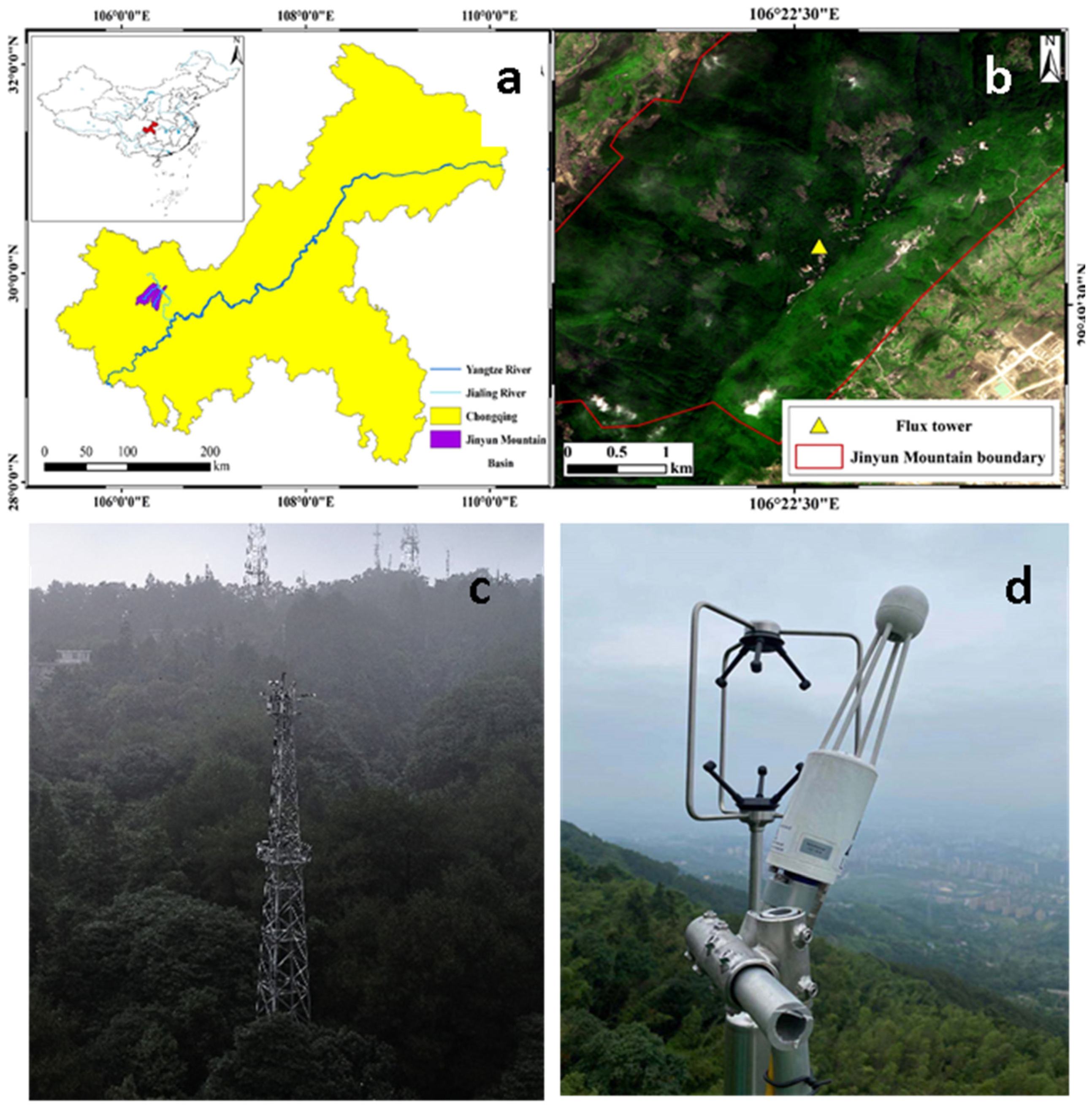
2.1. Study Area and Site Information

Jinyun Mountain is in Chongqing, Sichuan Basin, SWC, and has a typical subtropical monsoon climate. Under natural conditions, it should be dominated by typical evergreen broad-leaved forests. However, due to the long-term interference by and influence of human factors, it is no longer a simple evergreen broad-leaved forest; rather, it has formed artificial secondary forests such as subtropical coniferous and broad-leaved mixed forest, coniferous forest, and bamboo forest [33]. If the natural community in Jinyun Mountain is renewed for a long time, it will successively become a typical evergreen broad-leaved forest [34]. Considering the rapidly growing area of planted forests in China, more planted forests and natural forests will be intertwined in the future, and they will eventually form a complex stand composition, including natural growth and artificial planting, different growth maturity periods, and human intervention. Obviously, further knowledge is needed to understand the temporal dynamics of water and heat fluxes in complex stands, especially when the influencing factors of water and heat fluxes are different in different stands.
The study area is located in Jinyun Mountain National Nature Reserve (JYM, Figure 1) [35], the West Bank of Wentang Gorge of Jialing River in the upper reaches of the Three Gorges Reservoir area of the Yangtze River in SWC (29°41′–29°52′ N, 106°17′–106°24′ E). It has a subtropical humid monsoon climate, with an annual average precipitation, temperature, and relative humidity of 1611.8 mm, 16.3 °C, and 87%, respectively. The reserve covers an area of 76 km2, with an elevation ranging from 350 to 951.5 m. Most of the precipitation occurs during April–September, except for August, which is characterized by very high air temperatures and low precipitation. Due to the high relative humidity, the reserve experiences approximately 150 fog days annually (167 fog days in the period of this study). The average annual sunshine duration is 1293.9 h, accounting for only 25~35% of the whole year, making it one of the areas with the lowest sunshine duration in China [35,36,37].
The forest coverage of the reserve is 96.6%, which is mainly composed of coniferous and broad-leaved mixed forest, broad-leaved pure forests and some bamboo forests. The average canopy height of the reserve is approximately 20~25 m, with Pinus massoniana and Cunninghamia lanceolata as the dominant needle leaf species. Symplocas setchuensis, Castanopsis fargesii, Machilus lichuanensis, and Polyspora axillaris are the common broadleaf species in the Yangtze River basin, and these species are abundant in the reserve [35,38]. The average tree height in the experimental plot (50 m × 50 m) around the flux tower is 22 m, and the undergrowth shrubs are almost invisible, which is typical of mature coniferous and broad-leaved mixed forest plots. The reserve ecosystem has the characteristics of high elevation, high humidity, high canopy density, and heavy rainfall. Therefore, the ecosystem of the reserve can first be summarized as a high humidity mountain forest ecosystem (HHMF) [35,39]. Whether it can be called an STMCF ecosystem requires further research [29,30].

2.2. EC Measurements and Meteorological Measurements

In this study, a flux tower was built at 902 m above sea level in JYM, and its location is shown in Figure 1. On the flux tower, we installed two sets of EC observation systems: one 25 m (EC25) from the ground (slightly higher than the canopy height) and the other at 35 m (EC35) from the ground (slightly higher than 1.5 times the canopy height). The two EC systems were installed in May 2016. After one month of trial operation, the data became stable and could be used for research. Unfortunately, since August 2017, the two EC systems have suffered equipment damage and replacement, power failure, and voltage fluctuation caused by line corrosion. We lost all the data from the two EC systems in the first 10 months of 2018, the data from the EC35 system from February to September 2019, and the data from the EC25 system from April to July 2020. To verify the availability and reliability of the EC system in HHMF, we selected the data obtained from continuous observations of the two sets of EC systems from June 2016 to June 2017 for analysis and research.
Two EC systems were equipped with the same EC system instruments. Each system uses LI-7500-RS open-path infrared gas analyzers IRGA (LI-COR, Inc., Lincoln, NE, USA) to measure the flux density in the vortices transported upwards by the forest system. A Gill New Wind Master 3D sonic anemometer, GILL-WM (Gill Instruments, Lymington, UK), was used to measure the vertical transport velocity of these vortices. The LI-7500 and sonic anemometer data were collected at 10 Hz frequency and recorded on the SMARTFLUX (LI-COR, Inc., Lincoln, NE, USA) data logger module.
Net radiation (Rn) and photosynthetic photon flux densities (PPFD) were measured at each system using CNR4 net radiometer and LI-190SB quantum sensors (Kipp & Zonen, Delft, The Netherlands; LI-COR). Air temperature (Tair), relative humidity (RH), and thus VPD were measured at each system using the HMP155A temperature and relative humidity sensor (Vaisala, Helsinki, Finland). Each system was also equipped with a three-cup anemometer and wind vane (01003–5 R.M. Young Co., Traverse, MI, USA) to measure wind speed (WS) and wind direction in addition to the sonic anemometer. Precipitation (P) was measured at 2 m and 35 m above the ground surface using two TR-525USW tipping-bucket rain gauges (Texas Electronics, Campbell, CA, USA). Six self-calibrating soil heat flux sensors (HP01SC, Hukseflux Thermal Sensors B.V., Delft, The Netherlands) were installed at 5 cm depth below the soil surface, and each sensor was randomly and discretely distributed around the tower, in consideration of representativeness. Volumetric soil water content and soil temperature were measured by six TEROS11 soil moisture temperature sensors (Meter Group, Pullman, WA, USA) at depths of 5, 10, 20, 40, 60, and 80 cm. The soil moisture content in this study only uses the measured value of the 5 cm deep sensor. All meteorological variables were continuously recorded using two Xlite-9210 data loggers (Sutron Corporation, Sterling, VA, USA) at a sampling frequency of 30 s and averaged over each 30 min.

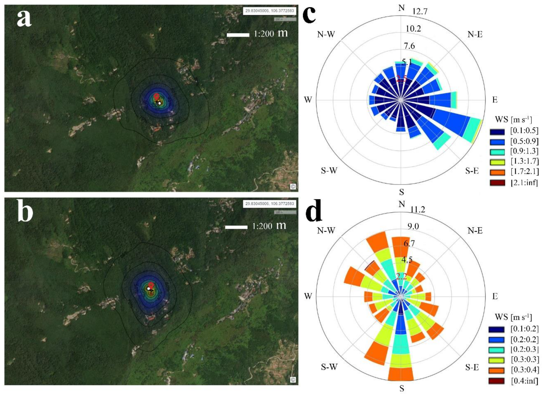
2.3. Data Processing, Screening, and Gap Filling of Fluxes

As recommended by previous studies, the raw 10 Hz EC data were processed using EddyPro software version 6.1.0 (LI-COR, Inc., Lincoln, NE, USA) in advanced mode to produce half-hourly fluxes of FEs [40,41,42,43,44,45,46,47,48]. According to the available research in the same type of region [49,50], in EddyPro, we used standardized correction procedures for high-frequency (10 Hz) data: axis rotation of tilt correction choosing double coordinate rotation [51], time-lag compensation using covariance maximization with default, 30-min block averaging, and statistical tests [52]; spike filtering and spectral correction [53,54,55]; anemometer temperature correction for humidity [56]; compensation for air density fluctuations [57]; data quality check using flagging policy 0-1-2 system [58,59]; and estimations of the flux footprint [60,61].
The processed EddyPro data were marked as three types: 0 (highest quality), 1 (normal quality), and 2 (lowest quality). Footprint analysis was carried out in TOVI version 2.8.1 (LI-COR, Inc., Lincoln, NE, USA) to generate a footprint contribution map and wind speed rose map (see Figure 2) [62]. The footprint map generated by TOVI software cannot display a 90% cumulative contribution area, and the 90% cumulative contribution distance was directly obtained from the data processed by EddyPro. Then, the REddyProcWeb online tool developed by the Max Planck Institute for Biogeochemistry (REddyProc: Eddy covariance data processing tool. Available online: https://www.bgc-jena.mpg.de/bgi/index.php/Services/REddyProcWeb (accessed on 16 May 2022)) was used to filter the friction velocity threshold of the processed EddyPro data [47]. The friction velocity threshold was estimated by a moving point test according to previous research, and the threshold of friction wind speed in this paper was 0.2 m·s−1 [63]. The flux data at all rainfall times were automatically filtered out by software and instruments. The fragmented quality-controlled flux data were then gap-filled using the REddyProcWeb online tool, and the percentages of the data filtered out were 22% and 21% for the EC25 and EC35 systems, respectively. Then, the partial continuous time series of flux after performing the standardized eddy covariance gap-filling methods was acquired [63]. The filling rate of the EC25 systems was 10% (daytime is 4% and nighttime is 6%), and that of the EC35 systems was 8% (daytime was 3% and nighttime was 5%). Due to the influence of rainfall and low turbulence, some data were continuously lost for more than several days, and the filling method could not fill well. To ensure the authenticity of the data, the continuous lost data lasting more than 3 days were not filled, but only the lost values on one day and on three consecutive days were filled. This may cause the annual cumulative evapotranspiration of the ecosystem to be underestimated, but in the study of the relationship between FEs and environmental factors, it helps to reduce the deviation caused by the interpolated data, because the interpolated FEs value was determined by the relationship with environmental factors.

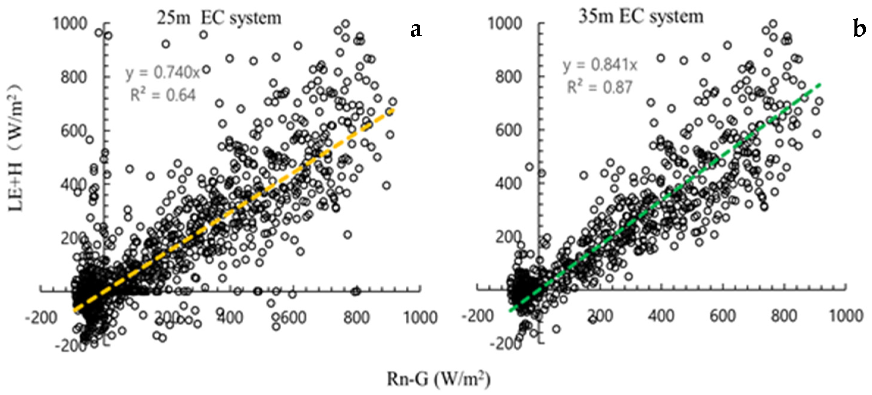
2.4. Energy Balance Closure

Energy balance closure (EBC) is widely used to evaluate the reliability and accuracy of EC measurements [64] and as an indirect way to check the accuracy of FE measurements. As highlighted by many previous studies, the surface energy balance can be written as follows [31,41,42,47,48,65,66,67]:
LE + H = Rn-G
LE + H = Rn-G-S
where Rn is the net solar radiation, G is the soil heat flux at a depth of 5 cm, H and LE are the sensible and latent heat fluxes, respectively, and S is the storage term including the sensible and latent heat storage values in the air layer. At present, there are two kinds of equations (Equations (1) and (2)) for the calculation of EBC. Equation (1) is convenient to calculate, but the EBC may be very low in some areas; in contrast, Equation (2) considers canopy heat storage, which will have a high EBC. Although the calculation method of S has many forms, it is still an estimated value rather than a measured value, which may cause some interference to the later proof of the applicability of the EC method in this region. In this paper, we adopted Equation (1) for calculation to ensure the authenticity and reliability of the research to the greatest extent. We computed the EBC from a linear regression between available energy Rn-G and the sums of turbulent fluxes (H + LE) using half-hourly values for the plant growing season. Recommended by previous studies, high-quality (0 flags) and non-gap filled fluxes of H and LE were used to calculate EBC only when all four components, H, LE, Rn, and G, were available [48].

2.5. Stepwise Regression Analysis of the Impacts of Changes in Environmental Driving Factors and Flux Exchange on HHMF

Stepwise regression is a way to build a model by adding or removing predictor variables, usually via a series of F tests or T tests. The variables to be added or removed are chosen based on the test statistics of the estimated coefficients [68]. Stepwise regression analysis is a part of multiple linear regression analysis. Multiple linear regression analysis emphasizes that there are multiple independent variables, and the independent variables and dependent variables are linear. This method can accurately measure the degree of correlation between various factors and the degree of regression fitting, which is widely used [69,70]. There are many ways for independent variables to enter the regression equation, and the stepwise entry method is one of them, so it is referred to as stepwise regression analysis. In addition to the step-by-step entry method, there are all entry methods, as well as forward and backwards methods [68]. Stepwise regression can eliminate irrelevant variables and ensure that there is no multicollinearity between the explanatory variables to obtain the optimal regression equation [71,72]. In a stepwise regression analysis, the relative importance of the variables for a given output can be evaluated through sensitivity indexes, including variables’ entry order to the model, SRCs (standardized regression coefficients)/SRRCs (standardized rank regression coefficients, for rank-transformed data), and R2 change attributable to the individual variables. The more important (sensitive) the variable is, the earlier it is selected into the linear model, the larger its SRC/SRRC is, and the more it is attributable to R2 change [73]. In this study, stepwise regression analysis was conducted to determine the drivers of FEs of HHMF. The variation in FEs was taken as the dependent variable, and the independent variables included the changes in six factors: air temperature (Tair), soil temperature (Tsoil), relative humidity (RH), wind speed (WS), radiation (Rn), and soil moisture (SM). First, we calculated the mean daily values of all of the variables; then, we standardized all variables. Finally, sampling points were imported into the stepwise regression tool in R (3.4.0) using F ≤ 0.05 as the selection criterion for each step. Each step was performed on the daily scale.
The stepwise regression model can be expressed as
Y = β 0 + β 1 X 1 + β 2 X 2 + · · · + β n X n + ε
where Y is the dependent variable—in this study, Y is the flux exchanges; Xi (i = 1, 2, 3···, n) is an independent variable—in this study, Xi is environmental factor; βi (i = 1, 2, 3···, n) is the regression coefficient, which is often solved by the least square method; ε is the residual—ε follows normal distribution. For the specific solution process, see multiple linear regression (Multiple linear regression. Available online: https://influentialpoints.com/Training/multiple_linear_regression-principles-properties-assumptions.htm (accessed on 16 May 2022)).

3. Results

3.1. Energy Balance Closure at HHMF

The EBC in this study was calculated for a one-year measurement period at heights of 25 m and 35 m of the flux tower in an HHMF. Both LE and H indicated a strong energy exchange between the canopy at EC25 m and the atmosphere measured at EC35 m. The EBC increased from 74% at the 25 m EC system to 84% at the 35 m EC system and averaged 79% across the two layers (Figure 3). The difference of EBC between the two-layer system may be mainly due to the different range of the contribution area caused by different measurement heights. Previous studies have shown that in complex underlying surfaces, such as forests, EBCs from 70% to 90% are considered satisfactory; because the theory of measurement problems is insufficient, there will be an energy imbalance ranging from 0% to 30% [74,75,76,77], and many EC studies in mountainous forests are within this range [47,78,79]. For energy imbalances in mountainous forest ecosystems, previous studies have shown that the mismatch between the EC footprint and other components of the surface energy balance (such as soil heat flux and net radiation) and the difficulty in obtaining accurate measurements of heat storage were the primary factors leading to energy imbalances in double-layer EC systems [80,81,82]. For this study, the roughness of the underlying surface as well as the high humidity and foggy environment were reasons explaining the unclosed energy. The errors do not mainly result from EC measurements, which lead to energy imbalance, and cannot correct the energy imbalance in this study, similar to previous studies [44,47,83,84,85]. Thus, FEs and ET will be analyzed in later studies without an energy imbalance correction.

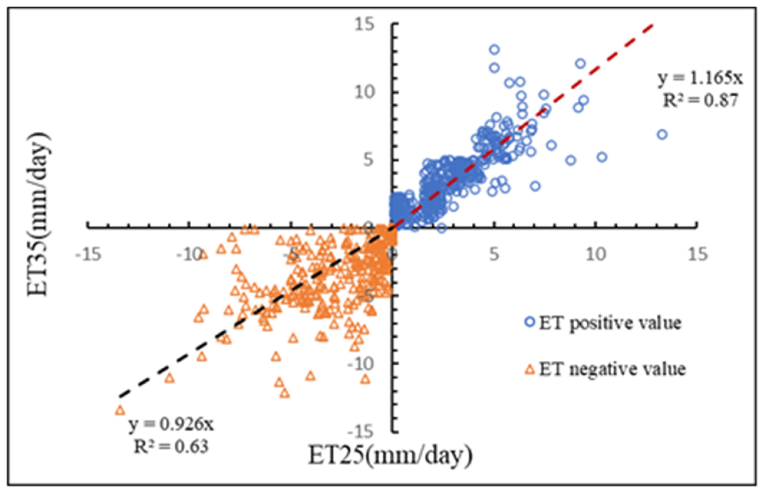
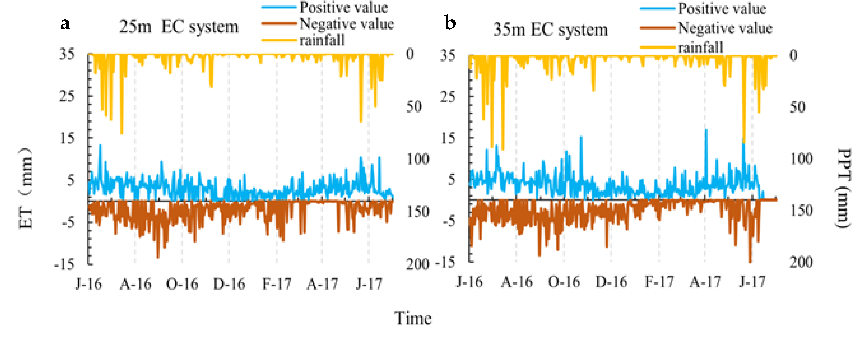
3.2. Evapotranspiration Comparison of the Two EC Systems

The ET measured at each layer, collected by the instrument directly and processed by Eddypro software, was calculated to be different from previous studies: the daily sum of ET was calculated, and the positive and negative values of each day ET were sorted and summed separately (Figure 4). The daily total ET measured by the two-layer EC system was different: for EC25, it ranged from −9.45 to 9.23 mm day−1, and at EC35, it ranged from −13.90 to 16.85 mm day−1. The negative and positive values of the daily ET were closed: for EC25, they were −13.40 and 13.27 mm day−1, while for EC35, they were −16.73 and 16.93 mm day−1. However, the annual ET of the two-layer EC system did not vary: the annual total, positive ET, and negative ET values at EC25 were 314.29, 1107.03, and −792.3 mm day−1, respectively, and those at EC35 were 389.31, 1387.76, and −998.45 mm day−1, respectively. Similar to previous studies [47,86,87,88], the comparison of daily ET from the EC25 and EC35 systems, which were used to further evaluate the reliability and representativeness of EC measurements in HHMF, is plotted in Figure 4. Linear regression analysis was conducted between the negative ET and positive ET from the EC25 and EC35 systems. The slopes of the regression analysis lines were 0.93 (R2 = 0.63, negative ET) and 1.17 (R2 = 0.87, positive ET), indicating very good agreement between the two EC systems.
However, without an energy imbalance correction, some differences were found between the annual ET of the two−layer EC systems. Thus, the energy imbalance of the EC measurements should be considered an error source in the study. In addition, the study used footprint models to perform footprint analysis for both EC systems [60,61] (Figure 2). For EC25, a 90% cumulative flux source contribution was in the range of 170.29 m around the flux tower, and a 90% cumulative flux source contribution was in the range of 298.47 m around the flux tower of EC35. The forest density around the flux tower was relatively constant; therefore, the annual ET from the EC35 system was slightly higher than that from the EC25 system due to the difference in footprint between the two EC systems. Previous studies indicated a good energy balance and highly correlated ET from the two EC systems, which had different footprints, and both proved that EC measurement was suitable for forest ecosystems in HHMF areas [47].

3.3. Characteristics of Annual Evapotranspiration

The annual ET of the two−layer EC system was not very different: the annual total, positive ET, and negative ET values measured by EC25 were 314.29, 1107.03, and −792.3 mm, respectively, while in EC35, the values were 389.31, 1387.76, and −998.45 mm, respectively (Figure 5). The annual precipitation (PPT), throughfall (TF), and canopy interception (CI) values were 1402.28, 1071.23, and 297.71 mm, respectively. The trunk runoff data (TR) were obtained from previous studies in the same period in the same area [35], and the CI calculation was as follows: CI = PPT − TF − TR. The annual transpiration (T), soil evaporation (SET), and annual average surface runoff (R) values were 812.44, 319.29, and 645.04 mm, respectively, in previous contemporaneous studies in the same area, in which T was measured by the sap flow method [35,89,90]. Both the positive and the negative ET values of the two−layer EC system had the same trend: the peak value of ET appeared in June and September, while the lowest value appeared in January (Figure 5). The annual PPT ranged from 0~90.68 mm, and the annual TF ranged from 0 to 75.67 mm. We assumed that all CIs were used for evaporation, and we found that the ET value measured by the sap flow method (ETSP) was 1429.44 mm (ETSP = T + SET + CI), which was close to that reported in a study with the same climatic conditions [18,91].

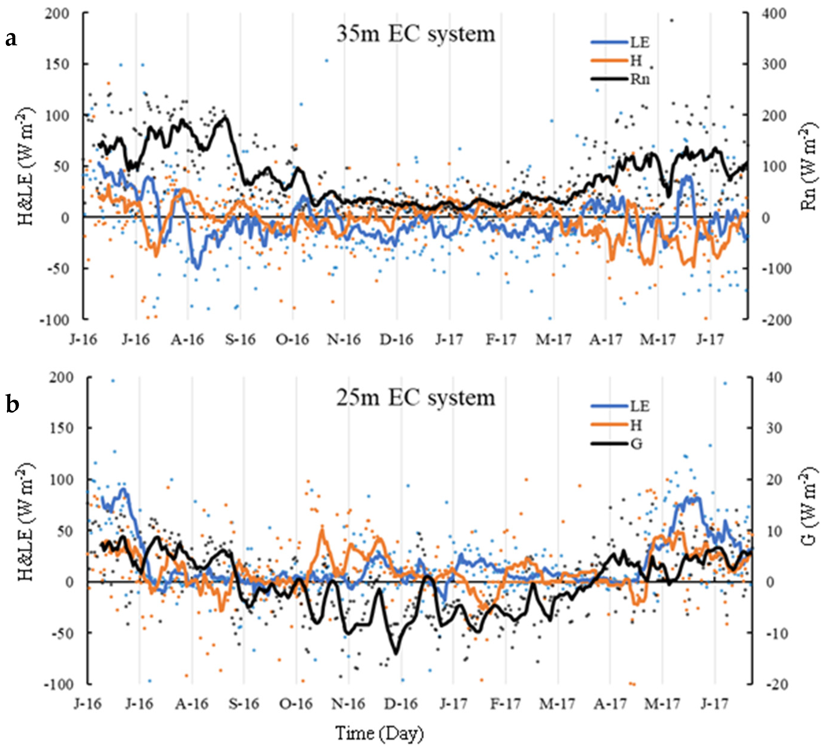
3.4. Energy Fluxes of the Two−Layer EC System

The daily mean LE in the two−layer EC system was slightly different: for the 25 m EC system, it ranged from −96.95~196.25 W m−2, and for the 35 m EC system, it ranged from −106.7 to 222.27 W m−2 (Figure 6). Daily mean H values were as follows: they ranged from −99.93~100.26 W m−2 at 25 m EC system, while that in the EC35 system ranged from −126.56 to 131.27 W m−2. The range of H was close to that of previous studies, but the range of LE was different in the high humidity forest ecosystems, ranging from −43~326.8 W m−2 (H) and −11.9~330.5 W m−2 (LE) [15,31,79]. The daily mean Rn at HHMF ranged within 0~385.60 W m−2, and the daily mean G ranged from −25.50~15.99 W m−2.

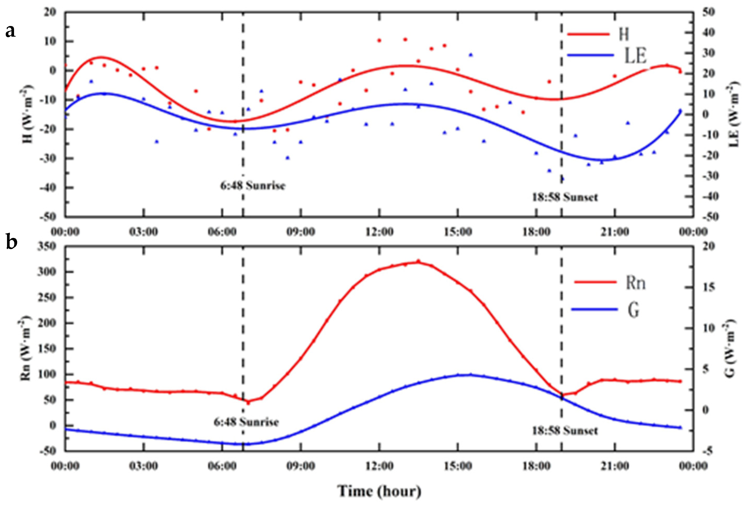
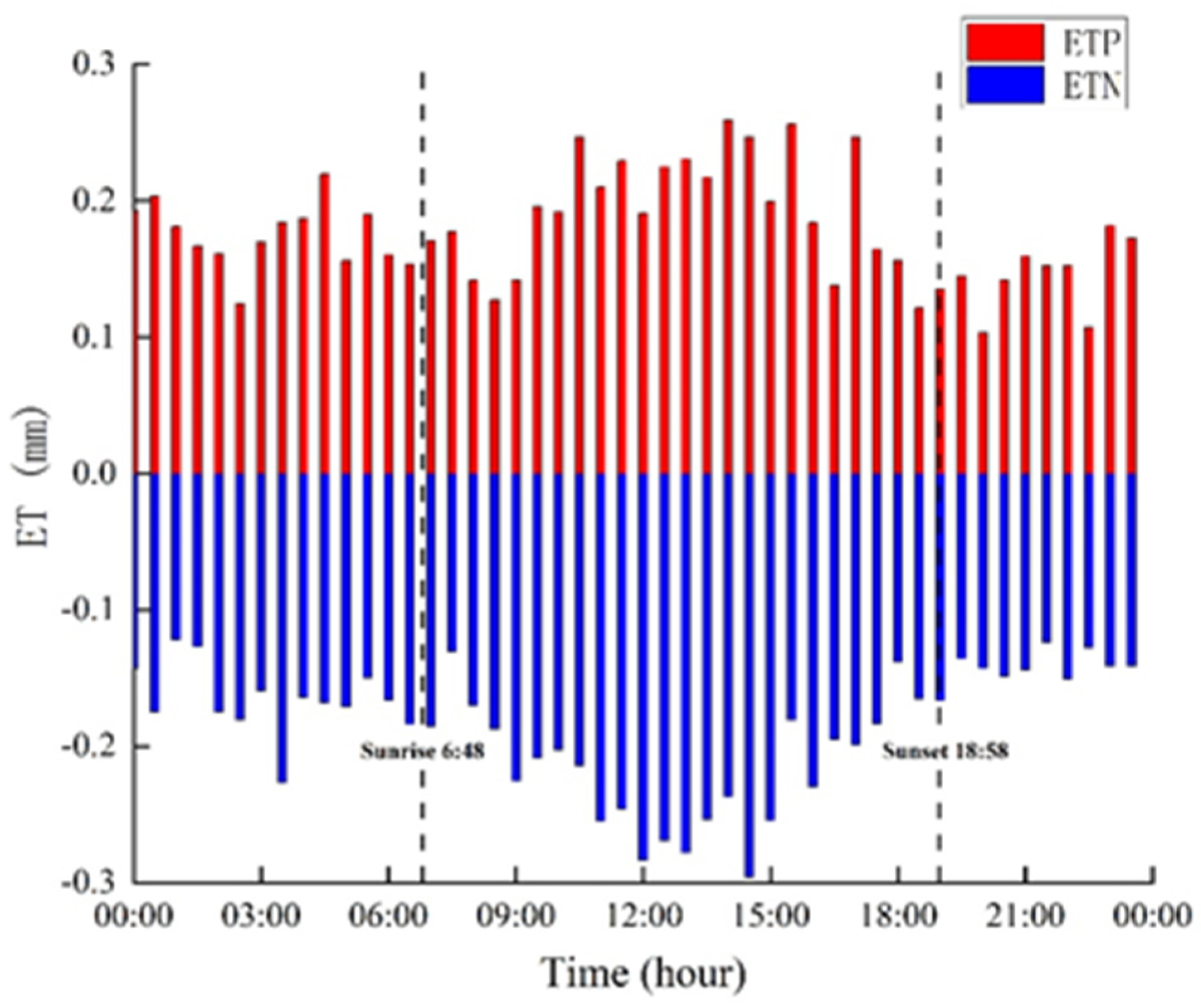
3.5. Characteristics of Hourly Energy and Water Flux

This study calculated the value of energy and water flux at the annual half−hour scale (Figure 7 and Figure 8) throughout the year. The hourly mean H and LE in the EC system were slightly different: for H, it ranged from −24.98~10.62 W m−2, and for LE, it ranged from −33.71 to 29.05 W m−2 (Figure 7). The highest value of H appeared at 12:00, and the highest value of LE appeared at 15:30. The lowest value of H appeared at 17:00, and the lowest value of LE appeared at 17:30. The highest value of Rn was 321.45 W m−2, which appeared at 13:30. The highest value of G appeared at 15:30, and the lowest value appeared at 7:00, which ranged from −4.16 to 4.31 W m−2. The ET of the half−hour scale throughout the year was divided into ETP and ETN (Figure 8). The hourly mean ETP and ETN in the EC system was slightly different: for ETP, it ranged from 0.10~0.26 mm, and for ETN, it ranged from −0.29~−0.12 mm. The highest value of ETP appeared at 14:00, and the highest value of ETN appeared at 1:30. The lowest value of ETP appeared at 20:00, and the lowest value of ETN appeared at 14:30.

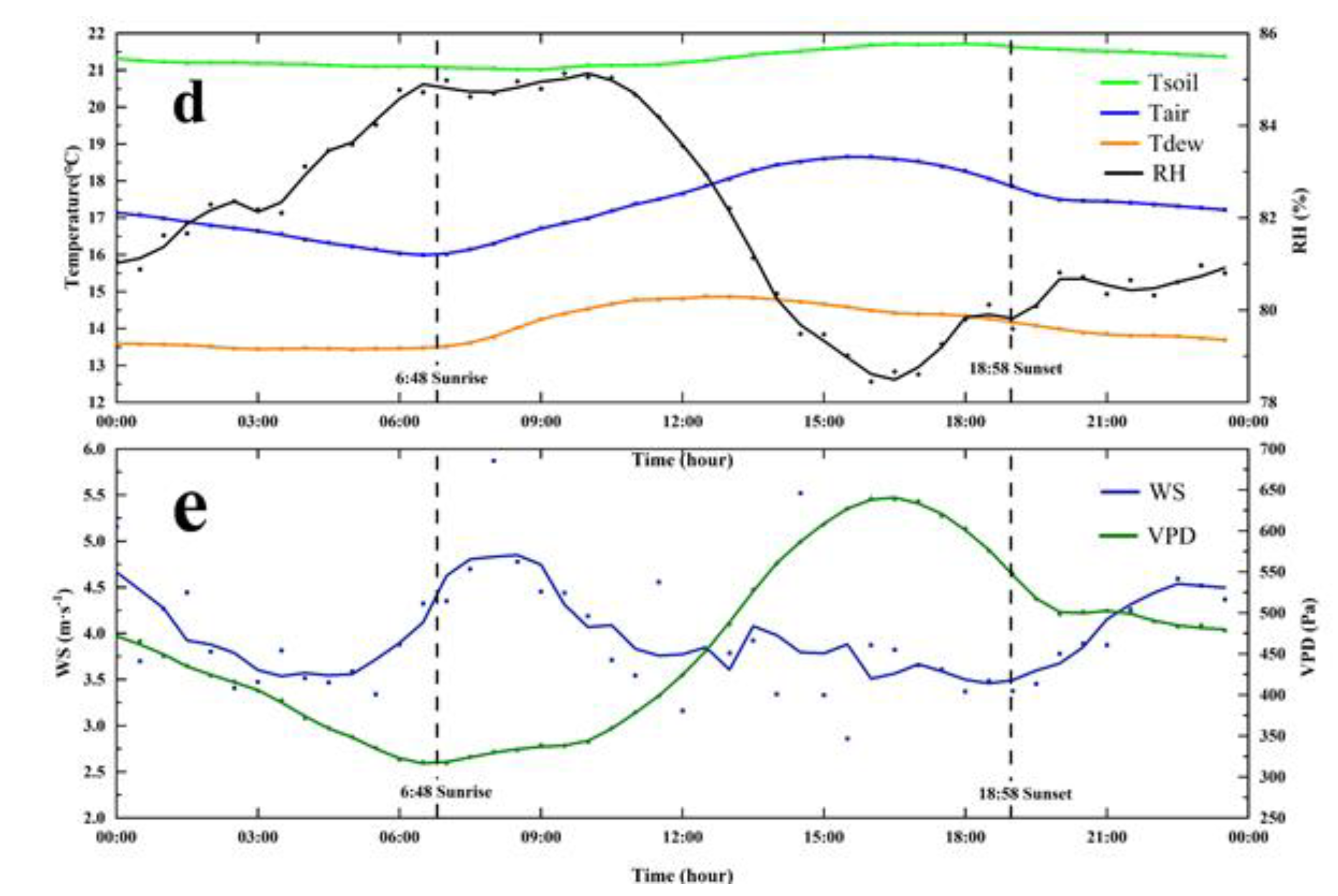
3.6. Characteristics of Annual Environmental Factors in HHMF

The variation characteristics of each environmental factor were as follows: to explore the effect of the day–night alternation on ET, this study calculated the value of each environmental factor at the daily scale (Figure 9a–c) and annual half−hour scale (Figure 9d,e) throughout the year. The annual mean sunrise and sunset times were 6:48 and 18:58 in Chongqing, respectively, and the annual mean daytime length was 12.16 h. The daily mean air temperature (Tair), dew point temperature (Tdew) and soil temperature (Tsoil) ranged from 1.56~31.75, −1.02~30.59, and 3.10~37.71 °C, respectively (Figure 9a); the daily mean relative humidity (RH) ranged from 36.48% to 100%, and the day when the minimum RH appeared was the day when there was no heavy rain for a long time (Figure 9d,e). The daily mean wind speed (WS) ranged from 0.91~4.99 m/s, the annual WS was 2.48 m s−1 (Figure 9b), and the daily mean vapor pressure deficit (VPD) ranged from 0–2144.81 Pa (Figure 9b). The day when the VPD was relatively high was the day when the RH was relatively low (Figure 9d,e).

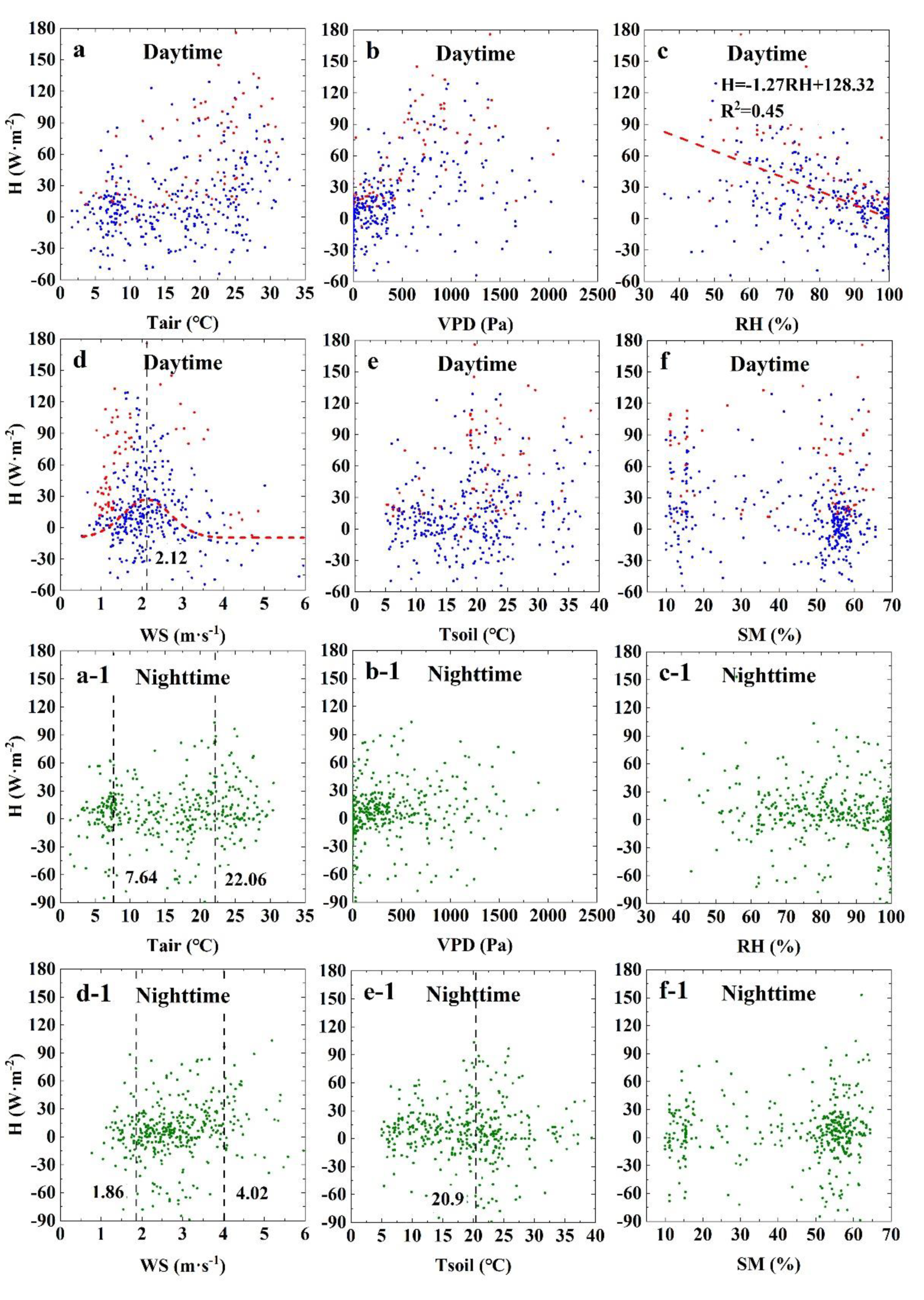
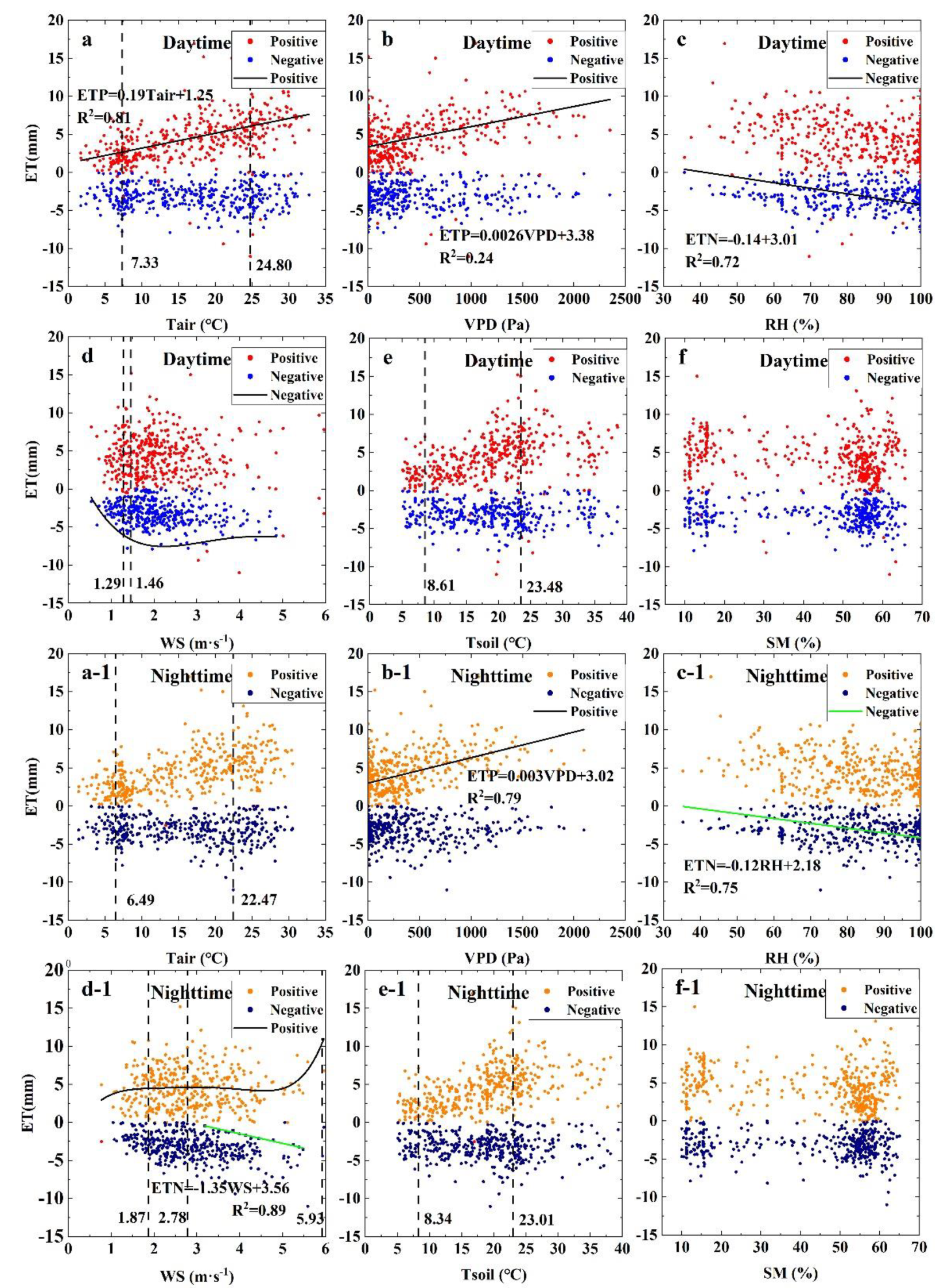
3.7. Response Characteristics of FEs to Environmental Factors

In this study, we analyzed the relationships between the Fes and six environmental factors (Tair, VPD, RH, WS, Tsoil, and SM), and each factor was divided into daytime and night (day: Figure 10a–f and Figure 11a–f; night: Figure 10a-1–f-1 and Figure 11a-1–f-1). The results showed that the daytime heat flux (D−H) increased with increases in Tair and VPD. However, the D−H was constrained by WS: for WS < 2.12 m s−1, D−H increased rapidly with increasing WS. For WS > 2.12 m s−1, the D−H increased negatively with increasing WS until it approached −21.81 W m−2 (Figure 10d). The results showed that the D−H had a good correlation with RH but not with Tsoil and SM (Figure 10c). In contrast, the night heat flux (N−H) had an apparent relationship with Tsoil, WS, and Tair. The three factors had three different strong restraint effects on N−H: for WS < 1.86 m s−1, WS limited N−H exchange, and only 10% of N−H occurred in this range; for WS ranging within 1.86~4.02 m s−1, 80% of N−H was distributed in this range; and for WS > 4.02 m s−1, WS also limited N−H exchange, and only 10% of N−H occurred in this range (Figure 10d-1). The correlation between N−H and Toil was not obvious, but the peak value appeared when Tsoil was 20.09 °C (Figure 10e-1). The N−H had two peaks with increasing Tair: the first peak appeared when Tair was 7.64 °C, and the second peak appeared when Tair was 22.06 °C (Figure 10a-1).
The positive value of evapotranspiration (ETP) linearly increased with rising Tair and VPD (Figure 11a-1 red plots). Similar to N−H, both daytime and night ETP (D−ETP and N−ETP) had certain rules with Tsoil but had two peaks with increasing Tsoil. The first D−ETP and N−ETP peaks occurred when Tsoil was 8.61 and 8.34 °C, respectively, and the second D−ETP and N−ETP peaks occurred when Tsoil was 23.48 and 23.01 °C, respectively (Figure 11e,e-1 red plots). The WS had different constraints on D−ETP and N−ETP. The relationship between D−ETP and WS was unimodal, and the peak value occurred when WS was 1.46 m s−1 (Figure 11d red plots). Unlike D−ETP, N−ETP rapidly increased when WS < 1.87 m s−1; for WS > 1.87 m s−1, N−ETP increased slightly until it reached 10.65 mm (Figure 11d-1 red plots). The negative value of evapotranspiration (ETN) was mainly affected by WS and RH. The daytime and night ETN (D−ETN and N−ETN) decreased with increasing RH (Figure 11c,c-1 red plot), and both were strongly constrained and had an obvious constraint line (for 0 < RH ≤ 100%, D−ETN: ET = −0.14RH + 3.01; N−ETN: ET = −0.12RH + 2.18). The D−ETN rapidly decreased when WS < 1.29 m s−1; for WS > 1.29 m s−1, the D−ETN decreased slightly and fluctuated near −5.65 mm (Figure 11d blue plot). WS had obvious constraints on N−ETN, for 2.78 < WS < 5.93 m s−1, and almost all points were below the line ET = −1.35 WS + 3.56 (Figure 11d-1 blue plot). Both D−ETN and N−ETN had two troughs with Tair: the first trough appeared when Tair was 7.33 °C (D−ETN) and 6.49 °C (N−ETN), and the second trough appeared when Tair was 24.80 °C (D−ETN) and 22.47 °C (N−ETN) (Figure 11a-1). The D−ETN and N−ETN were also constrained by a single peak of Tsoil and VPD, but the relationships were not strong (Figure 11c,e,c-1,e-1). There was no direct relationship between ETN and SM (Figure 11f,f-1).

3.8. Environmental Driving Forces of FEs under Circadian Alternation in HHMF

The linear stepwise regression analysis was used to analyze the relationship between seven environmental factors (Rn, Tair, VPD, RH, Tsoil, WS, SM) and FEs under two scenarios (daytime and nighttime) (Table 1).

3.8.1. Driving Forces of H Change

To facilitate the comparative analysis with previous studies, we incorporated Rn into the analysis. The D−H exhibited a relatively good R2 compared with the N−H; among the seven environmental driving forces, Rn, RH, and WS had very high significance (Table 1). There was no significant correlation in Tair, VPD, Tsoil, and SM. The change in the D−H was mainly influenced by Rn, and the regression coefficient (RC) was 0.379 higher than the RC absolute values of RH and WS. The RCs of WS and RH were negative, indicating that they had a negative effect on H. The correlation between the N−H and environmental driving forces was weak (R2 = 0.069). The VPD and SM showed good significance in the N−H, and their RC was closed, indicating that H was affected by both.

3.8.2. Driving Forces of ETP Change

The D−ETP and N−ETP exhibited relatively good and closed R2 values, indicating that the environmental driving forces had a strong influence on them (Table 1). For the D−ETP, Rn, Tair, and WS had relatively good significance. In contrast to the D−H, the change in the D−ETP was mainly affected by Tair (RC = 0.393). The N−ETP change was mainly influenced by the driving forces of Tair, VPD, RH, and Tsoil. The RC of the VPD was the highest (RC = 0.560), which indicated that the N−ETP change was strongly influenced by the VPD.

3.8.3. Driving Forces of ETN Change

The D−ETN and N−ETN exhibited relatively general R2 values, indicating that the effect of environmental forces on ETN was nonlinear (Table 1). The Tair, RH, and WS had obvious significance in the D−ETN and N−ETN. The RC of WS was the highest in the D−ETN and N−ETN, indicating that WS was the main driving force of ETN change. The RC of RH in the D−ETN was close to the WS, which showed that RH was the secondary driving force of the D−ETN change. There was no significant correlation between ETN and VPD, Tsoil, and SM, but there were some restraints by these forces (Figure 11).

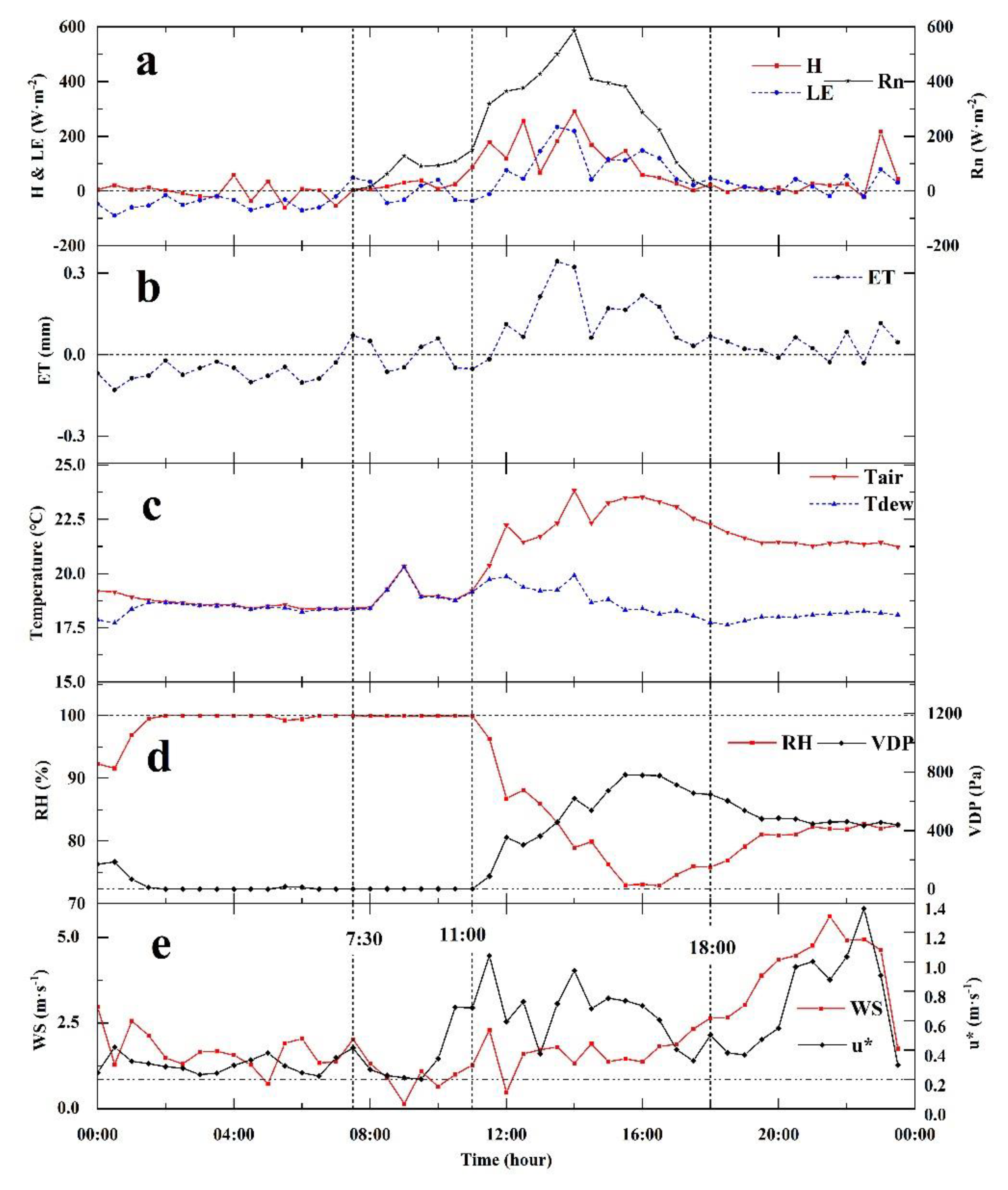
3.9. Specific Analysis on Foggy Days

Previous studies have shown that when the relative humidity continues at 100%, the water vapor will reach the supersaturation state, resulting in the emergence of fog periods [92,93]. To ensure the occurrence of fog during the study period, in this study, only days with a relative humidity of 100% for many hours were selected for specific fog analysis. In addition, the selected date had continuous half−hour scale raw data without interpolation to ensure the accuracy of the study. Similar to the previous research on the specific case analysis of fog, two days with different periods of fog were selected for research [92,93,94]. On one day, the fog appeared before 11:00 a.m (22 October 2016) (Figure 12); on another, fog appeared after 10:00 a.m (3 June 2017) (Figure 13).
The daily variation characteristics of FEs and environmental factors on 22 October 2016 were as follows (Figure 12): H, LE, and RN were in the range of −60.14~291.86, −88.87~233.56, and 3.68~585.20 W m−2, respectively. ET was in the range of −0.13~0.34 mm. Tair and Tdew were in the range of 18.37~23.83 and 17.65~20.29 °C, respectively. RH and VPD were in the range of 72.87~100% and 0~780.52 Pa, respectively. WS and u* were in the range of 0.14~5.61 and 0.20~1.36 m·s−1, respectively.
The daily variation characteristics of FEs and environmental factors on 3 June 2017 were as follows (Figure 13): H, LE, and RN were in the range of −35.15~146.96, −152.66~130.26, and 1.79~291.39 W m−2, respectively. ET was in the range of −0.22~0.19 mm. Tair and Tdew were in the range of 20.04~23.82 and 15.19~21.19 °C, respectively. RH and VPD were in the range of 58.69~100% and 0~1213.80 Pa, respectively. WS and u* were in the range of 0.31~5.76 and 0.20~1.03 m·s−1, respectively.

4. Discussion

4.1. Application of EC System in HHMF

The water flux and energy balance of the high humidity forest ecosystem in the Jinyun Mountain National Nature Reserve were studied by using a two−layer EC system. Previous research used the double−layer EC observation system to prove that under the complex underlying surface conditions [47], the system could also carry out quantitative observation and research, which was quite different from the homogeneous underlying surface conditions of most flux studies [65,95,96,97]. In this study, the energy closure, footprint model and ET of the 35 m and 25 m EC systems were analyzed by using the double−layer EC observation system. Figure 1 shows the energy closure of the 35 m and 25 m EC systems, and both observational EC systems exhibited high energy closure rates. Figure 2 shows the analysis results of the footprint model and the direction of the main contribution area of wind direction. Figure 3 shows the comparison of ET between the 25 m and 35 m EC observation systems. The ET measured by the two−layer EC system was linearly regressed. The slope of the linear regression line of ETP was 1.17 and that of ETN was 0.92, all fluctuating near 1 (1 represents the same value), indicating that the two−layer EC system had quite good agreement in ET. The farthest distance of the 90% cumulative flux contribution of the 25 m EC system was 170.29 m, and that of the 35 EC system was 298.47 m; additionally, the longest distance of the upper EC system was 1.75 times that of the lower EC system at the same location.
Previous studies have shown that the best position for the EC instrumentation was in the constant flux layer, located approximately 1.5~2 times the height of the canopy above the soil surface but below the mixed layer (100–150 m above the soil surface) [75,97,98]. The canopy height of the forest ecosystem in JYM ranges from 22 to 24 m; therefore, the effective range of the 25 m EC system was limited, and the measurement results can represent only the flux exchange in a very small range around the instrument. However, we believe that the smaller the measurement range, the closer the measured value is to the real value. The height of the 35 m EC system in this study was close to twice the height of the tree canopy, so it could be considered that the measurement results of this height were enough to represent the flux exchange between the ecosystem and the outside atmosphere. The energy closure, ET, and footprints of the two EC systems had good responses, which meant that the fluxes from different footprints were quite consistent in JYM. This result showed that the distribution of different types of forests in the JYM ecosystem was relatively uniform, the influence of topographic fluctuations on the EC system could be ignored, and the measurement results of the EC system were quite representative of the whole watershed.

4.2. Water Balance and Energy Exchange of HHMF

Using the EC system, we preliminarily estimated the water balance of JYM. The annual total ET of EC35 was 389.31 mm, that of EC25 was 314.29 mm, and the T measured by the sap flow method in the same period was 812.44 mm [35]. The serious mismatch between ET and T indicated that there were many negative values in ET that could not be ignored. By calculating the positive and negative values of ET separately, we found that 44.4% of the negative values existed in the ET measured by the 35 m EC system, and 49.1% were measured in the 25 m EC system. Since the footprint range of the 35 m EC system was more suitable for the whole basin, we used the ET measured by the 35 m EC system in the water balance calculation. After calculation, T accounted for 58.6% of the ETP, which was similar to the results of a previous study on the relationship between ET and T, indicating that the ETP was the real ET measured by the EC system [99,100,101]. Using only the ETP in the water balance calculation, we calculated that the annual water consumption measured by the EC (WCEC) of the basin was 2032.80 mm (WCEC = ETP + R), which was greater than the annual PPT of the basin (PPT = 1402.28 mm), and the water budget of the basin was seriously unbalanced. In addition, the annual water consumption measured by the sap flow method (WCSP) was 2074.48 mm (WCSP = ETSP + R), and there was also an obvious water imbalance. Both methods showed that the ecosystem has another way to obtain water from the atmosphere other than rainfall. Therefore, it was necessary to consider adding the absolute value of ETN (|ETN|) to the water balance calculation. Through the calculation, we found that the water supplement (WTS) amount of the basin was 2400.73 mm (WTS = PPT + |ETN|). The WTS was slightly larger than the WCEC and WCSP, indicating that the watershed had a good water balance, which was more in line with the local situation of heavy rain and high humidity. With nearly half of the ET measurements and a good water balance in the basin, the ETN had a very high research ability in the basin and was an important link in the water cycle of the basin. It is worth mentioning that the positive and negative values of ET measured by the EC system represent the flow direction of water vapor in the direction: the positive value represented the water vapor output from the ecosystem to the atmosphere, and the negative value represented the water vapor input from the atmosphere to the ecosystem.

4.3. Specific Fog Case Analysis

Many studies have shown that fog is a phenomenon in which water vapor condenses into water droplets under the influence of environmental factors [102,103,104,105], which is an inverse process of ET that can be observed by EC systems. In addition, many studies have shown that when the relative humidity is above 90%, there is a 50% probability of fog; if the temperature is around 10 °C, the probability of fog is close to 100% [106,107]. To ensure the occurrence of fog in the specific case analysis, according to the previous research on a cloud forest in Taiwan [92,93,94], this study used a date when the relative humidity was at 100% for several consecutive hours in a day. Before 11 a.m. on 22 October 2016, the half−hour values of Tair and Tdew were almost identical, and the relative humidity was close to 100%, which jointly indicated that fog occurred before 11 a.m. (Figure 12c,d). The same situation occurred after 10 a.m. on 3 June 2017, which also indicated that fog occurred after 10 a.m. (Figure 13c,d). At the beginning, the fog appears with a RH gradually increasing from less than 90% to close to 100% (before 7:30 in Figure 12a,b and between 10:00 and 13:30 in Figure 13a,b), and both ET and LE were observed as negative values, indicating that water vapor flowed into the ecosystem from the atmosphere. During the daytime, when RH fluctuated near 100% for a long time (between 7:30 and 11:00 in Figure 12a,b and between 16:30 and 20:00 in Figure 13a,b), indicating the persistence of fog, ET and LE were affected by radiation, and both positive and negative values were observed. In the fog disappearance stage when RH was less than 100% and gradually decreased (between 11:00 and 18:00 in Figure 12a,b and before 10:00 am and between 13:30 and 16:30 in Figure 13a,b), ET and LE observations were both positive. In the process of relative humidity rising from 70% to more than 80% at night (Figure 12 after 18:00), the positive and negative values of ET and LE observed by EC appeared. On the night when the relative humidity fluctuated at 100%, indicating the persistence of fog (Figure 13 after 20:00), the ET and LE observed by EC were negative and decreased continuously. In addition, the friction wind speed (u*) on the two selected days was greater than 0.2 m·s−1, indicating that the turbulence was still within the reasonable observation range when the fog occurred, which showed that the FEs observed by EC technology during the study period were reliable (Figure 12e and Figure 13e). The results of this study were similar to those of fog observation in a cloud forest in Taiwan. When RH increased from a small value to 100%, the flux direction observed by EC was mainly the downward process of turbulent deposition to the ecosystem. When the relative humidity exceeds 100% and the water vapor in the air reaches the critical supersaturation, droplets of different sizes will exist at the same time and be affected by radiation. Droplets of medium and lower sizes will be subject to upward turbulence, which was observed as positive by EC, and droplets of larger sizes will be deposited into the ecosystem, which was observed as negative by EC. When the relative humidity drops below 100%, the droplets will evaporate and shrink to the size of their balance with the surrounding air. Therefore, the EC system will observe the upward process of water vapor flux [92,94]. The analysis of fog events on two different dates in this study shows that this is not a process that only occurs in a single event or rarely occurs. Moreover, similar patterns were also observed in the analysis of multiple fog events [92,93,94].
In addition, by dividing the half−hour rainfall data according to an RH greater than 90%, the rainfall frequency in fog was 93.7%, accounting for 90.5% of the total rainfall. Combined with the actual situation that the observation tower is at a higher altitude on the top of the mountain and the cloud layer is relatively low, and so the fog will appear before and after rainfall, we believe that it was credible to classify fog time according to a relative humidity greater than 90%. According to statistics, the half−hour scale ET data during the study period were divided according to a relative humidity greater than 90%, showing that 44.6% of the study period had fog; ETN accounted for 64.1% of ET in foggy time and only 42.3% in fogless time. Combined with the specific case analysis of foggy days, most of the ETN observed by EC system in this study was sinking fog, and the other part did not appear in the form of fog but was also affected by RH. Moreover, many studies have shown that fog participates in a unique hydrological cycle in tropical, subtropical, and coastal areas. A great quantity of fog supplied water vapor to other systems every year, providing a unique water source [108,109,110,111,112,113]. Therefore, the forest ecosystem in this study area can be called sub−tropical mountain cloud forest (STMCF) [28,29].

4.4. Effects of Environmental Factors on FEs in HHMF

The H and LE had similar trends in the two−layer EC system. In autumn and winter, they both changed strongly, hovering around zero. This result may be due to the foggy season in autumn and winter in this area, and the water vapor in the air was almost saturated, meaning that the subtle energy change could cause the sharp change in H and LE. The characteristics of high humidity and fog in this area caused H to not increase with RN in the growing season. Especially from April to June 2017, due to the arrival of the rainy season, the temperature and humidity changed strongly, which made H fluctuate strongly (Figure 6).
To study the impact of environmental factors on FEs, we first processed the environmental data, on average, for every half hour throughout the year. Through the local latitude data, we obtained the annual average sunrise time (6:48) and sunset time (18:58). Both RH and Tair had obvious responses to day–night alternations. After sunrise, the growth trend of RH slowed and began to decrease rapidly from 11:00 until 16:30, and RH began to increase gradually (Figure 9d). Tair began to increase after sunrise, peaked at 16:00, and then began to decline until sunrise. The temperature difference between Tdew and Tair narrowed after sunset, and the difference was the smallest near sunrise, indicating that water vapor condensation was more likely to occur before sunrise. There was a similar trend between the VPD and TAIR. After sunrise, the VPD began to increase gradually until it reached its peak at 16:30 (Figure 9e). Combining RH and VPD with Tair, we found that temperature had a significant effect on the RH and VPD in this area. When the night temperature decreased, the RH increased gradually, and the VPD decreased gradually, which indicated that a large amount of water vapor was condensed at night, which was the main cause of the negative water flux observed by the EC system. In addition, the influence of elevation on climate factors in this area should not be ignored [114,115,116]. Specifically, compared with previous studies on the RH and Tair in the Chongqing urban area [117,118], we found that there was a 30% difference in RH and a 5 °C difference in Tair between the urban area and study area. This result could also explain the change in RH and VPD before sunset (at 16:30). In terms of the annual scale, RH had a high average value in autumn and winter, VPD had a low average value in same period, and both factors indicated that there would be a large amount of fog condensation in the cold months as the water source in HHMF, which could explain why there was still a large amount of ET when there was little precipitation in winter. (Figure 5 and Figure 9a,b). As March, April, and August are typical dry months in the study area, with the characteristics of less rainfall and higher temperature, the VPD and RH changed significantly in these months. In addition, compared with other dry months, the radiation in August was stronger, so the VPD had the highest value of the whole year. May and June of each year are the key rain seasons in the study area, with weak radiation and frequent rainfall. Therefore, RH can increase rapidly and VPD decreases rapidly in these months, resulting in a large amount of fog, and the study area will be in the alternating process of fog and rainfall throughout the month, which is characterized by fog in the day and rain at night (Figure 9a,b,). WS had no obvious seasonal variation at the annual scale but had a certain variation trend at the daily scale. At sunrise and sunset, WS had an increasing trend, which was mainly due to the temperature difference between the urban area and the study area at sunrise and sunset and the strong convection under the joint action of radiation and altitude (Figure 9d,e)
Through the daily and annual scale analysis of environmental factors, we clearly found that environmental factors had different change trends during the day and at night. Therefore, to further explore the relationship between FEs and environmental factors, we divided the environmental factors and FEs into both day and night (Figure 10 and Figure 11).
According to previous studies [47,119], we analyzed the relative contribution of seven environmental factors to FEs (RN was added considering the daytime conditions) using multiple stepwise regression Table 1). As expected, during the daytime, we found that the H change was mainly affected by radiation (Rn), the change in ETP was mainly affected by temperature (Tair), and the exchange of ETN was affected by both relative humidity (RH) and wind speed (WS). At night, the H changes were affected by the vapor pressure deficit (VPD) and soil moisture (SM), the ETP changes were mainly related to the VPD, and the ETN exchange was mainly affected by the WS. In this study, the ETP, as the actual ET in HHMF, was mainly affected by Tair during the day and by VPD at night. The results confirm previous studies that found that the main influencing factors of ET in ecosystems were not Rn but were other environmental factors. For example, the ET of an alpine meadow ecosystem on the Qinghai Tibet Plateau was mainly determined by Tair, and H was mainly affected by Rn [119]; Similarly, the ET change in the Xishuangbanna tropical rainforest ecosystem in Southwest China was mainly related to Tair [15]. However, the ET change in a tropical peat forest ecosystem in Malaysia was related to the VPD [66]. The ET in the subtropical primary evergreen forest ecosystem of Ailao Mountain in Southwest China was also mainly controlled by the VPD, which additionally showed that fog plays an important role in the eco−hydrological system and deserves further investigation [17]. Through the comprehensive analysis of the above examples and this study, we found that in tropical or subtropical areas, there should be two main environmental factors (Tair and VPD) that have an impact on the change in ET rather than a single environmental factor. Perhaps other studies will show a similar conclusion after the separation of day and night. Therefore, this study suggests that the separation of day and night should be carried out in future studies of ET. From the analysis of energy exchange, the changes in H and LE (ETP) during the day are affected by radiation and temperature, indicating that ecosystem energy is limited during the day. If the energy−related factors change, the FE mechanism may change [119,120,121].
In the study of circadian alterations, the ETN was mainly controlled by WS and secondarily controlled by RH (Figure 11 and Table 1). Because the ETP increased with increasing temperature and the |ETN| increased with increasing wind speed, when ET (ET = ETP + ETN) was not divided into positive and negative values, especially when ETP > ETN resulted in ET > 0 on the daily scale, it was difficult to find the emergence of ETN. If Tair and WS increased at the same time, the growth rate of ETN may have been greater than ETP; that is, at the same time, the amount of water vapor output from the ecosystem to the atmosphere was gradually equal to the amount of water vapor input from the atmosphere to the ecosystem, and gradually in dynamic equilibrium. As a result, Tair increased while ET decreased. In other words, we found that the negative contribution of WS to ET would offset the positive contribution of Tair. This result can provide a good research direction for the observed decrease of actual ET in the evaporation paradox; that is, the idea that global warming may lead to the increase of evaporation potential is inconsistent with the observed fact that the actual evaporation in the world, especially in the northern hemisphere, has decreased significantly. When the research time scale is long, such as on a multi−year scale, the ET value on the day scale or the ET value on the longer time scale is usually used (when using remote sensing to study et, an ET value is usually obtained in 8 days or 16 days). In this case, the observation accuracy of ET is not enough. Thus, the interference of ETN to the study of long−time series cannot be ruled out, resulting in the fact that the observed ET does not meet the expected value. This result is strikingly similar to previous studies on reference evapotranspiration (ET0) in the five provinces in Southwest China, the Qinghai–Tibetan Plateau, the three−river source region, and the arid area of Iran but opposite to those in the Pearl River Delta, northern Xinjiang, and the southwestern United States [122,123,124,125,126,127,128]. Therefore, in the study of ET, we also suggest splitting the positive and negative values of ET before the study.
To specifically explore the reasons for the impact of WS on ETN, we consider that it is the result of the joint action of altitude difference and radiation change. The low−altitude urban area is in the subtropical zone and surrounded by the Jialing River, which has a typical urban heat island effect and a high−temperature and high−humidity environment. Therefore, a large amount of humid and hot air flows rising in the urban area will sink and collect in the high−altitude research area with relatively low temperature, forming a mountain wind with fog. The flow of the wind will remove the heat in the research area, further reduce the temperature, and positively promote the formation of fog. In addition, this process is more obvious when the temperature difference is large, such as at sunrise, sunset, and night. This result meets the previous research results in many regions. For example, forest research in the mountainous area of northern Thailand showed that there was a certain functional relationship between fog and wind [129]. In the Lushan Mountain forest in China, a higher wind speed was conducive to fog condensation [130]. In the coastal area of southern China, the formation of fog required low wind speed and small turbulent kinetic energy, and fog formation was promoted by having the energy flux downwards at night with the land surface cooling the atmosphere as well as having lower soil temperature and higher soil humidity [130]. In the greater Zagreb region, downhill winds contributed to the continuous formation of fog [131]. In the arid area of southwestern Morocco, the location of the city relative to the Atlas Mountains was the main factor affecting the generation of dew [132]. Overall, we found that the heat island effect in the urban area played an important role in water condensation in the study area.

4.5. Limitation and Constraints

Due to the influence of data observation, this study can only use the data of one year to study ET. It was found that the negative ET decreases with the increase of temperature, which may lead the observed ET to have decreased with the increased of temperature, which was similar to the phenomenon of evaporation paradox. Due to the lack of multi−year flux observation data, this study cannot deeply study the causes of the evaporation paradox. However, this study provided a new research direction and method for the phenomenon of evaporation paradox; that is, the increase of temperature may increase the frequency of negative ET observed by EC method in various regions, which may be one of the reasons for the emergence of the evaporation paradox phenomenon.
In this study, the preliminary reliable data were obtained through data quality control and friction wind speed threshold processing, and then the analysis of energy closure rate further proved that the EC method was applicable in this region. During the study of ET, it was accidentally found that there will be a large amount of negative ET in the study area, which may be related to fog. Therefore, when installing EC observation equipment, this study area lacked the consideration of relevant professional equipment for fog observation, so the depth analysis of the relationship between fog and evapotranspiration was still lacking, especially the specific relationship between fog and negative evapotranspiration in the case of low turbulence. However, through the analysis of reliable observation data after quality control, this study shows that the EC method can also be applicable in foggy periods. Through the preliminary study of foggy periods by EC method, this area can be defined as a subtropical cloud forest area, which is rare in subtropical areas.

5. Conclusions

Based on the observation of the double—layer EC system, we proved the applicability of the EC system in HHMF. The results showed that good energy closure, different footprint contribution ranges, and good consistency between the two EC systems jointly proved that the EC system was quite suitable in HHMF. By using two methods for water balance, we found that fog was observed by the EC system in the form of negative ET as a reverse ET process. Thus, fog is an important water source of HHMF that cannot be ignored and conforms to the definition of a cloud forest. Therefore, we defined the highly humid forest ecosystem in this study area as a subtropical mountain cloud forest (STMCF).
Through the daily scale study of environmental factors, we found that it is necessary to separate day and night when further studying the relationship between FEs and environmental factors. Stepwise regression analysis of environmental factors and FEs showed that during the day, the changes in H and LE (ETP) were mainly affected by radiation and temperature; at night, the changes in ETP were mainly affected by VPD, but the changes in ETN were affected by WS all day. As a result, the ecosystem was energy−limited during the day (affected by radiation and temperature), and future climate warming may enhance the FEs of the ecosystem. Heat island cities in subtropical regions play an important role in water vapor condensation in nearby mountains. Further intensification of the heat island effect may lead to more water vapor condensation in the study area in the future.
In general, we suggest that day and night separation and positive and negative value separation should be carried out in future ET research to explore the influencing factors of ET in more detail and help us to understand more phenomena, such as the evaporation paradox. In the future research, this study area will use professional instruments to observe the fog and deeply analyze the relationship between the emergence of fog and negative evapotranspiration. In addition, future studies will use long time—scale evapotranspiration data to explore whether the new research method of the evaporation paradox provided by this paper is feasible.

Author Contributions

Conceptualization, K.W. and Y.W. (Yunqi Wang); methodology, K.W.; software, K.W.; investigation, S.W.; resources, Y.W. (Yujie Wang); data curation, J.W. and Y.F.; writing—original draft preparation, K.W.; writing—review and editing, K.W and Y.W. (Yunqi Wang); visualization, K.W.; supervision, Y.W. (Yunqi Wang); project administration, Y.W. (Yunqi Wang); funding acquisition, Y.W. (Yujie Wang) All authors have read and agreed to the published version of the manuscript.

Funding

This study was supported by the Hot Spot Tracking Project of Beijing Forestry University, Ecological Protection, and Restoration Management of the Upper Reaches of Yangtze River (2021BLRD05).

Institutional Review Board Statement

Not applicable.

Informed Consent Statement

Not applicable.

Data Availability Statement

The data presented in this study are available on request from the corresponding author. The data are not publicly available due to privacy or ethical restrictions.

Conflicts of Interest

The authors declare no conflict of interest.

References

  1. IPCC, 2019: IPCC Special Report on the Ocean and Cryosphere in a Changing Climate. Available online: https://www.ipcc.ch/srocc/ (accessed on 8 March 2022).
  2. Pörtner, H.O.; Roberts, D.C.; Tignor, M.; Poloczanska, E.S.; Mintenbeck, K.; Alegría, A.; Craig, M.; Langsdorf, S.; Löschke, S.; Möller, V.; et al. (Eds.) IPCC, 2022: Climate Change 2022: Impacts, Adaptation, and Vulnerability; Contribution of Working Group II to the Sixth Assessment Report of the Intergovernmental Panel on Climate Change; Cambridge University Press: Cambridge, UK, 2022. [Google Scholar]
  3. Vitasse, Y.; Signarbieux, C.; Fu, Y.H. Global warming leads to more uniform spring phenology across elevations. Proc. Natl. Acad. Sci. USA 2018, 115, 1004–1008. [Google Scholar] [CrossRef] [PubMed] [Green Version]
  4. Cahill, A.E.; Aiello-Lammens, M.E.; Caitlin Fisher-Reid, M.; Hua, X.; Karanewsky, C.J.; Ryu, H.Y.; Sbeglia, G.C.; Spagnolo, F.; Waldron, J.B.; Warsi, O.; et al. How does climate change cause extinction? Proc. R. Soc. B Biol. Sci. 2013, 280, 20121890. [Google Scholar] [CrossRef] [PubMed]
  5. Grimm, N.B.; Chapin, F.S.; Bierwagen, B.; Gonzalez, P.; Groffman, P.M.; Luo, Y.; Melton, F.; Nadelhoffer, K.; Pairis, A.; Raymond, P.A.; et al. The impacts of climate change on ecosystem structure and function. Front. Ecol. Environ. 2013, 11, 474–482. [Google Scholar] [CrossRef] [Green Version]
  6. Allen, C.D.; Macalady, A.K.; Chenchouni, H.; Bachelet, D.; McDowell, N.; Vennetier, M.; Kitzberger, T.; Rigling, A.; Breshears, D.D.; Hogg, E.H.; et al. A global overview of drought and heat-induced tree mortality reveals emerging climate change risks for forests. For. Ecol. Manag. 2010, 259, 660–684. [Google Scholar] [CrossRef] [Green Version]
  7. Haddeland, I.; Heinke, J.; Biemans, H.; Eisner, S.; Flörke, M.; Hanasaki, N.; Konzmann, M.; Ludwig, F.; Masaki, Y.; Schewe, J.; et al. Global water resources affected by human interventions and climate change. Proc. Natl. Acad. Sci. USA 2014, 111, 3251–3256. [Google Scholar] [CrossRef] [Green Version]
  8. Hock, R.; Rasul, C.; Adler, B.; Cáceres, S.; Gruber, Y.; Hirabayashi, M.; Jackson, A.; Kääb, S.; Kang, S.; Kutuzov, A.; et al. 2019: High Mountain Areas. IPCC Special Report on the Ocean and Cryosphere in a Changing Climate. Available online: https://www.ipcc.ch/site/assets/uploads/sites/3/2019/11/06_SROCC_Ch02_FINAL.pdf (accessed on 8 March 2022).
  9. Zhang, C.; Ren, Y.; Cao, L.; Wu, J.; Zhang, S.; Hu, C.; Zhujie, S. Characteristics of Dry-Wet Climate Change in China during the Past 60 Years and Its Trends Projection. Atmosphere 2022, 13, 275. [Google Scholar] [CrossRef]
  10. Lin, L.; Ge, E.; Chen, C.; Luo, M. Mild weather changes over China during 1971–2014: Climatology, trends, and interannual variability. Sci. Rep. 2019, 9, 2419. [Google Scholar] [CrossRef]
  11. Zhang, Y.-D.; Zhang, X.-H.; Liu, S.-R. Correlation analysis on normalized difference vegetation index (NDVI) of different vegetations and climatic factors in Southwest China. Ying Yong Sheng Tai Xue Bao J. Appl. Ecol. 2011, 22, 323–330. [Google Scholar]
  12. Shan, H.; Yang, Y.; Hanjia, W.; Qidong, Y. Spatio-temporal Characteristics of Sensible and Latent Heat Flux in Southwest China. J. Arid Meteorol. 2020, 38, 601–611. [Google Scholar]
  13. Zhu, X.J.; Yu, G.R.; Wang, Q.F.; Hu, Z.M.; Zheng, H.; Li, S.G.; Sun, X.M.; Zhang, Y.P.; Yan, J.H.; Wang, H.M.; et al. Spatial variability of water use efficiency in China’s terrestrial ecosystems. Glob. Planet. Chang. 2015, 129, 37–44. [Google Scholar] [CrossRef]
  14. Li, Z.; Zhang, Y.; Wang, S.; Yuan, G.; Yang, Y.; Yu, G.; Sun, X. Evaluating the models of stomatal conductance response to humidity in a tropical rain forest of xishuangbanna, southwest China. Hydrol. Res. 2011, 42, 307–317. [Google Scholar] [CrossRef]
  15. Li, Z.; Zhang, Y.; Wang, S.; Yuan, G.; Yang, Y.; Cao, M. Evapotranspiration of a tropical rain forest in Xishuangbanna, southwest China. Hydrol. Process. 2010, 24, 2405–2416. [Google Scholar] [CrossRef]
  16. Zhang, Y.; Tan, Z.; Song, Q.; Yu, G.; Sun, X. Respiration controls the unexpected seasonal pattern of carbon flux in an Asian tropical rain forest. Atmos. Environ. 2010, 44, 3886–3893. [Google Scholar] [CrossRef]
  17. Song, Q.H.; Braeckevelt, E.; Zhang, Y.P.; Sha, L.Q.; Zhou, W.J.; Liu, Y.T.; Wu, C.S.; Lu, Z.Y.; Klemm, O. Evapotranspiration from a primary subtropical evergreen forest in Southwest China. Ecohydrology 2017, 10, e1826. [Google Scholar] [CrossRef]
  18. Lin, Y.; Wang, G.X.; Guo, J.Y.; Sun, X.Y. Quantifying evapotranspiration and its components in a coniferous subalpine forest in Southwest China. Hydrol. Process. 2012, 26, 3032–3040. [Google Scholar] [CrossRef]
  19. Song, Q.H.; Fei, X.H.; Zhang, Y.P.; Sha, L.Q.; Wu, C.S.; Lu, Z.Y.; Luo, K.; Zhou, W.J.; Liu, Y.T.; Gao, J.B. Snow damage strongly reduces the strength of the carbon sink in a primary subtropical evergreen broadleaved forest. Environ. Res. Lett. 2017, 12, 104014. [Google Scholar] [CrossRef] [Green Version]
  20. Santamouris, M. Analyzing the heat island magnitude and characteristics in one hundred Asian and Australian cities and regions. Sci. Total Environ. 2015, 512, 582–598. [Google Scholar] [CrossRef]
  21. Stewart, I.D.; Oke, T.R. Local climate zones for urban temperature studies. Bull. Am. Meteorol. Soc. 2012, 93, 1879–1900. [Google Scholar] [CrossRef]
  22. He, B.J.; Ding, L.; Prasad, D. Relationships among local-scale urban morphology, urban ventilation, urban heat island and outdoor thermal comfort under sea breeze influence. Sustain. Cities Soc. 2020, 60, 102289. [Google Scholar] [CrossRef]
  23. Rajagopalan, P.; Lim, K.C.; Jamei, E. Urban heat island and wind flow characteristics of a tropical city. Sol. Energy 2014, 107, 159–170. [Google Scholar] [CrossRef]
  24. Papanastasiou, D.K.; Kittas, C. Maximum urban heat island intensity in a medium-sized coastal Mediterranean city. Theor. Appl. Climatol. 2012, 107, 407–416. [Google Scholar] [CrossRef]
  25. Huang, L.P.; Miao, J.F.; Liu, Y.K. Spatial and temporal variation characteristics of urban heat island in Tianjin. Trans. Atmos. Sci. 2012, 35, 620–632. [Google Scholar]
  26. Yow, D.M. Urban heat islands: Observations, impacts, and adaptation. Geogr. Compass 2007, 1, 1227–1251. [Google Scholar] [CrossRef]
  27. Li, L.; Liang, Z.; Wang, H.; Li, C.; Wang, X.; Zhao, X. Urban heat island characteristics in Shenyang under different weather conditions. Trans. Atmos. Sci. 2011, 34, 8. (In Chinese) [Google Scholar]
  28. Mathez-Stiefel, S.L.; Peralvo, M.; Báez, S.; Rist, S.; Buytaert, W.; Cuesta, F.; Fadrique, B.; Feeley, K.J.; Groth, A.A.P.; Homeier, J.; et al. Research Priorities for the Conservation and Sustainable Governance of Andean Forest Landscapes. Mt. Res. Dev. 2017, 37, 323–339. [Google Scholar] [CrossRef] [Green Version]
  29. Bubb, P.; May, I.; Miles, L.; Sayer, J. Cloud Forest Agenda; UNEP: Nairobi, Kenya, 2004; pp. 1–36. [Google Scholar]
  30. Williams-Linera, G. El Bosque de Niebla del Centro de Veracruz: Ecología, Historia y Destino en Tiempos de Fragmentación y Cambio Climático; Instituto de Ecología: Xalapa, Mexico, 2007. [Google Scholar]
  31. Domínguez-Eusebio, C.A.; Alarcón, E.; Briones, O.L.; del Rosario Pineda-López, M.; Perroni, Y. Surface energy exchange: Urban and rural forest comparison in a tropical montane cloud forest. Urban For. Urban Green. 2019, 41, 201–210. [Google Scholar] [CrossRef]
  32. Groffman, P.M.; Cadenasso, M.L.; Cavender-Bares, J.; Childers, D.L.; Grimm, N.B.; Grove, J.M.; Hobbie, S.E.; Hutyra, L.R.; Darrel Jenerette, G.; McPhearson, T.; et al. Moving Towards a New Urban Systems Science. Ecosystems 2017, 20, 38–43. [Google Scholar] [CrossRef]
  33. Xu, S.; Zeng, B.; Su, X.; Lei, S.; Liu, J. Spatial distribution of vegetation and carbon density in Jinyun Mountain nature reserve based on RS/GIS. Shengtai Xuebao/Acta Ecol. Sin. 2012, 32, 2174–2184. [Google Scholar] [CrossRef] [Green Version]
  34. Yu, T. Investigation on vegetation status in Jinyun Mountain. Dajiang Wkly. Forum 2013, 7, 52. (In Chinese) [Google Scholar]
  35. Zhang, X.; Wang, Y.; Wang, Y.; Zhang, S.; Zhao, X. Effects of social position and competition on tree transpiration of a natural mixed forest in Chongqing, China. Trees-Struct. Funct. 2019, 33, 719–732. [Google Scholar] [CrossRef]
  36. Yu, L.; Wang, Y.; Wang, Y.; Sun, S.; Liu, L. Quantifying components of soil respiration and their response to abiotic factors in two typical subtropical forest stands, southwest China. PLoS ONE 2015, 10, e0117490. [Google Scholar] [CrossRef] [PubMed] [Green Version]
  37. Liu, N.; Wang, Y.; Wang, Y. Effect of subtropical forests on water quality in Southwestern China. Afr. J. Agric. Res. 2011, 6, 6354–6362. [Google Scholar] [CrossRef]
  38. Weide, S. The Classification and Ordination of the Forest Communities of the Jinyun Mountain, Sichuan Province. Chin. J. Plant Ecol. 1983, 7, 299–312. [Google Scholar]
  39. Shen, T.; Corlett, R.T.; Song, L.; Ma, W.Z.; Guo, X.L.; Song, Y.; Wu, Y. Vertical gradient in bryophyte diversity and species composition in tropical and subtropical forests in Yunnan, SW China. J. Veg. Sci. 2018, 29, 1075–1087. [Google Scholar] [CrossRef]
  40. Chi, J.; Waldo, S.; Pressley, S.; O’Keeffe, P.; Huggins, D.; Stöckle, C.; Pan, W.L.; Brooks, E.; Lamb, B. Assessing carbon and water dynamics of no-till and conventional tillage cropping systems in the inland Pacific Northwest US using the eddy covariance method. Agric. For. Meteorol. 2016, 218–219, 37–49. [Google Scholar] [CrossRef] [Green Version]
  41. Aguiar, R.G.; De Musis, C.R.; Aguiar, L.J.G.; Martínez-Espinosa, M.; Fischer, G.R. Energy balance closure in the Southwest Amazon forest site—A statistical approach. Theor. Appl. Climatol. 2019, 136, 1209–1219. [Google Scholar] [CrossRef]
  42. Heusinger, J.; Weber, S. Surface energy balance of an extensive green roof as quantified by full year eddy-covariance measurements. Sci. Total Environ. 2017, 577, 220–230. [Google Scholar] [CrossRef]
  43. Fortuniak, K.; Pawlak, W.; Bednorz, L.; Grygoruk, M.; Siedlecki, M.; Zieliński, M. Methane and carbon dioxide fluxes of a temperate mire in Central Europe. Agric. For. Meteorol. 2017, 232, 306–318. [Google Scholar] [CrossRef]
  44. Zhou, Y.; Xiao, X.; Wagle, P.; Bajgain, R.; Mahan, H.; Basara, J.B.; Dong, J.; Qin, Y.; Zhang, G.; Luo, Y.; et al. Examining the short-term impacts of diverse management practices on plant phenology and carbon fluxes of Old World bluestems pasture. Agric. For. Meteorol. 2017, 237–238, 60–70. [Google Scholar] [CrossRef] [Green Version]
  45. Chen, B.; Chamecki, M.; Katul, G.G. Effects of Gentle Topography on Forest-Atmosphere Gas Exchanges and Implications for Eddy-Covariance Measurements. J. Geophys. Res. Atmos. 2020, 125, e2020JD032581. [Google Scholar] [CrossRef]
  46. Tang, A.C.I.; Stoy, P.C.; Hirata, R.; Musin, K.K.; Aeries, E.B.; Wenceslaus, J.; Melling, L. Eddy Covariance Measurements of Methane Flux at a Tropical Peat Forest in Sarawak, Malaysian Borneo. Geophys. Res. Lett. 2018, 45, 4390–4399. [Google Scholar] [CrossRef] [Green Version]
  47. Tie, Q.; Hu, H.; Tian, F.; Holbrook, N.M. Comparing different methods for determining forest evapotranspiration and its components at multiple temporal scales. Sci. Total Environ. 2018, 633, 12–29. [Google Scholar] [CrossRef] [PubMed]
  48. Anapalli, S.S.; Fisher, D.K.; Reddy, K.N.; Krutz, J.L.; Pinnamaneni, S.R.; Sui, R. Quantifying water and CO2 fluxes and water use efficiencies across irrigated C3 and C4 crops in a humid climate. Sci. Total Environ. 2019, 663, 338–350. [Google Scholar] [CrossRef] [PubMed]
  49. Zhu, Z.; Sun, X.; Zhou, Y.; Xu, J.; Yuan, G.; Zhang, R. Correcting method of eddy covariance fluxes over non-flat surfaces and its application in ChinaFLUX. Sci. China Ser. D Earth Sci. 2005, 48, 42–50. [Google Scholar] [CrossRef]
  50. Bi, X.Y.; Wen, B.; Zhao, Z.K.; Huang, J.; Liu, C.X.; Huang, H.J.; Mao, W.K.; Wen, G.H. Evaluation of corrections on turbulent fluxes obtained by eddy covariance method in high winds. J. Trop. Meteorol. 2018, 24, 176–184. [Google Scholar] [CrossRef]
  51. Wilczak, J.M.; Oncley, S.P.; Stage, S.A. Sonic anemometer tilt correction algorithms. Bound.-Layer Meteorol. 2001, 99, 127–150. [Google Scholar] [CrossRef]
  52. Vickers, D.; Mahrt, L. Quality control and flux sampling problems for tower and aircraft data. J. Atmos. Ocean. Technol. 1997, 14, 512–526. [Google Scholar] [CrossRef]
  53. Moncrieff, J.; Clement, R.; Finnigan, J.; Meyers, T. Averaging, Detrending, and Filtering of Eddy Covariance Time Series. In Handbook of Micrometeorology; Springer: Dordrecht, The Netherlands, 2006; pp. 7–31. [Google Scholar] [CrossRef]
  54. Moncrieff, J.B.; Massheder, J.M.; de Bruin, H.; Elbers, J.; Friborg, T.; Heusinkveld, B.; Kabat, P.; Scott, S.; Soegaard, H.; Verhoef, A. A system to measure surface fluxes of momentum, sensible heat, water vapour and carbon dioxide. J. Hydrol. 1997, 188–189, 589–611. [Google Scholar] [CrossRef]
  55. Mauder, M.; Foken, T. Impact of post-field data processing on eddy covariance flux estimates and energy balance closure. Meteorol. Z. 2006, 15, 597–609. [Google Scholar] [CrossRef]
  56. van Dijk, A.; Moene, A.F.; de Bruin, H.A.R. The Principles of Surface Flux Physics: Theory, Practice and Description of the Library; Meteorology and Air Quality Group, Wageningen University: Wageningen, The Netherlands, 2004. [Google Scholar]
  57. Webb, E.K.; Pearman, G.I.; Leuning, R. Correction of flux measurements for density effects due to heat and water vapour transfer. Q. J. R. Meteorol. Soc. 1980, 106, 85–100. [Google Scholar] [CrossRef]
  58. Mauder, M.; Foken, T. Documentation and Instruction Manual of the Eddy-Covariance Software Package TK3. Arbeitsergebnisse 2011, 46, 60. [Google Scholar]
  59. Mauder, M.; Cuntz, M.; Drüe, C.; Graf, A.; Rebmann, C.; Schmid, H.P.; Schmidt, M.; Steinbrecher, R. A strategy for quality and uncertainty assessment of long-term eddy-covariance measurements. Agric. For. Meteorol. 2013, 169, 122–135. [Google Scholar] [CrossRef]
  60. Kormann, R.; Meixner, F.X. An analytical footprint model for non-neutral stratification. Bound.-Layer Meteorol. 2001, 99, 207–224. [Google Scholar] [CrossRef]
  61. Kljun, N.; Calanca, P.; Rotach, M.W.; Schmid, H.P. A simple parameterisation for flux footprint predictions. Bound.-Layer Meteorol. 2004, 112, 503–523. [Google Scholar] [CrossRef]
  62. Kljun, N.; Calanca, P.; Rotach, M.W.; Schmid, H.P. A simple two-dimensional parameterisation for Flux Footprint Prediction (FFP). Geosci. Model Dev. 2015, 8, 3695–3713. [Google Scholar] [CrossRef] [Green Version]
  63. Papale, D.; Reichstein, M.; Aubinet, M.; Canfora, E.; Bernhofer, C.; Kutsch, W.; Longdoz, B.; Rambal, S.; Valentini, R.; Vesala, T.; et al. Towards a standardized processing of Net Ecosystem Exchange measured with eddy covariance technique: Algorithms and uncertainty estimation. Biogeosciences 2006, 3, 571–583. [Google Scholar] [CrossRef] [Green Version]
  64. Anemometer, S.; Measurements, T.F.; Analyser, I.G. Advances in Ecological Research Volumes 1–23. Adv. Ecol. Res. 2000, 24, 408–410. [Google Scholar] [CrossRef]
  65. Zhou, Y.; Li, X. Energy balance closures in diverse ecosystems of an endorheic river basin. Agric. For. Meteorol. 2019, 274, 118–131. [Google Scholar] [CrossRef]
  66. Tang, A.C.I.; Stoy, P.C.; Hirata, R.; Musin, K.K.; Aeries, E.B.; Wenceslaus, J.; Shimizu, M.; Melling, L. The exchange of water and energy between a tropical peat forest and the atmosphere: Seasonal trends and comparison against other tropical rainforests. Sci. Total Environ. 2019, 683, 166–174. [Google Scholar] [CrossRef]
  67. Pereira, A.R.; Angelocci, L.; Sentelhas, P. Agrometeorologia: Fundamentos e aplicações práticas. Agrometeorol. Fundam. E Apl. Práticas 2002, 11, 123. [Google Scholar]
  68. Wang, G.C.S.; Jain, C.L. Regression Analysis: Modeling & Forecasting; Institute of Business Forec: Great Neck, NY, USA, 2003; ISBN 0932126502. [Google Scholar]
  69. Dong, X.; Li, F.; Lin, Z.; Harrison, S.P.; Chen, Y.; Kug, J.S. Climate influence on the 2019 fires in Amazonia. Sci. Total Environ. 2021, 794, 148718. [Google Scholar] [CrossRef] [PubMed]
  70. Chen, Y.; Randerson, J.T.; Morton, D.C.; Defries, R.S.; Collatz, G.J.; Kasibhatla, P.S.; Giglio, L.; Jin, Y.; Marlier, M.E. Forecasting fire season severity in South America using sea surface temperature anomalies. Science 2011, 334, 787–792. [Google Scholar] [CrossRef] [PubMed] [Green Version]
  71. Hao, R.; Yu, D.; Liu, Y.; Liu, Y.; Qiao, J.; Wang, X.; Du, J. Impacts of changes in climate and landscape pattern on ecosystem services. Sci. Total Environ. 2017, 579, 718–728. [Google Scholar] [CrossRef] [PubMed]
  72. Desboulets, L.D.D. A review on variable selection in regression analysis. Econometrics 2018, 6, 45. [Google Scholar] [CrossRef] [Green Version]
  73. Saltelli, A.; Tarantola, S.; Campolongo, F.; Ratto, M. Sensitivity Analysis in Practice: A Guide to Assessing Scientific Models; Wiley Online Library: Hoboken, NJ, USA, 2004; Volume 1. [Google Scholar]
  74. Liu, X.; Yang, S.; Xu, J.; Zhang, J.; Liu, J. Effects of soil heat storage and phase shift correction on energy balance closure of paddy fields. Atmosfera 2017, 30, 39–52. [Google Scholar] [CrossRef]
  75. Burba, G. Eddy Covariance Method-for Scientific, Industrial, Agricultural, and Regulatory Applications. 2013. Available online: https://books.google.co.uk/books?hl=zh-CN&lr=&id=8lPB-H4IR9EC&oi=fnd&pg=PA7&dq=Eddy+Covariance+Method-for+Scientific,+Industrial,+Agricultural,+and+Regulatory+Applications&ots=cHEsoAuGLa&sig=2jyjLAkIxK3OCkZ9YU4ih2bRqis#v=onepage&q=Eddy%20Covariance%20Method-for%20Scientific%2C%20Industrial%2C%20Agricultural%2C%20and%20Regulatory%20Applications&f=false (accessed on 8 March 2022).
  76. Foken, T.; Aubinet, M.; Leuning, R. The Eddy Covariance Method. Eddy Covariance 2012, 11, 1–19. [Google Scholar] [CrossRef]
  77. Twine, T.E.; Kustas, W.P.; Norman, J.M.; Cook, D.R.; Houser, P.R.; Meyers, T.P.; Prueger, J.H.; Starks, P.J.; Wesely, M.L. Correcting eddy-covariance flux underestimates over a grassland. Agric. For. Meteorol. 2000, 103, 279–300. [Google Scholar] [CrossRef] [Green Version]
  78. Shimizu, T.; Kumagai, T.; Kobayashi, M.; Tamai, K.; Iida, S.; Kabeya, N.; Ikawa, R.; Tateishi, M.; Miyazawa, Y.; Shimizu, A. Estimation of annual forest evapotranspiration from a coniferous plantation watershed in Japan (2): Comparison of eddy covariance, water budget and sap-flow plus interception loss. J. Hydrol. 2015, 522, 250–264. [Google Scholar] [CrossRef]
  79. Chu, H.S.; Chang, S.C.; Klemm, O.; Lai, C.W.; Lin, Y.Z.; Wu, C.C.; Lin, J.Y.; Jiang, J.Y.; Chen, J.; Gottgens, J.F.; et al. Does canopy wetness matter? Evapotranspiration from a subtropical montane cloud forest in Taiwan. Hydrol. Process. 2014, 28, 1190–1214. [Google Scholar] [CrossRef]
  80. Leuning, R.; van Gorsel, E.; Massman, W.J.; Isaac, P.R. Reflections on the surface energy imbalance problem. Agric. For. Meteorol. 2012, 156, 65–74. [Google Scholar] [CrossRef]
  81. Stoy, P.C.; Katul, G.G.; Siqueira, M.B.S.; Juang, J.Y.; Novick, K.A.; Mccarthy, H.R.; Oishi, A.C.; Uebelherr, J.M.; Kim, H.S.; Oren, R. Separating the effects of climate and vegetation on evapotranspiration along a successional chronosequence in the southeastern US. Glob. Chang. Biol. 2006, 12, 2115–2135. [Google Scholar] [CrossRef] [Green Version]
  82. Wilson, K.; EnWilson, K. Energy balance closure at FLUXNET sites. Agric. For. Meteorol. 2002, 113, 223–243. [Google Scholar] [CrossRef] [Green Version]
  83. Waldo, S.; Chi, J.; Pressley, S.N.; O’Keeffe, P.; Pan, W.L.; Brooks, E.S.; Huggins, D.R.; Stöckle, C.O.; Lamb, B.K. Assessing carbon dynamics at high and low rainfall agricultural sites in the inland Pacific Northwest US using the eddy covariance method. Agric. For. Meteorol. 2016, 218–219, 25–36. [Google Scholar] [CrossRef] [Green Version]
  84. Zhang, Z.; Tian, F.; Hu, H.; Yang, P. A comparison of methods for determining field evapotranspiration: Photosynthesis system, sap flow, and eddy covariance. Hydrol. Earth Syst. Sci. 2014, 18, 1053–1072. [Google Scholar] [CrossRef] [Green Version]
  85. Anapalli, S.S.; Fisher, D.K.; Reddy, K.N.; Wagle, P.; Gowda, P.H.; Sui, R. Quantifying soybean evapotranspiration using an eddy covariance approach. Agric. Water Manag. 2018, 209, 228–239. [Google Scholar] [CrossRef]
  86. Song, T.; Sun, Y.; Wang, Y. Multilevel measurements of fluxes and turbulence over an urban landscape in Beijing. Tellus B Chem. Phys. Meteorol. 2013, 65, 20421. [Google Scholar] [CrossRef]
  87. Liu, Y.; Liu, H.; Du, Q.; Xu, L. Multi-level CO2 fluxes over Beijing megacity with the eddy covariance method. Atmos. Ocean. Sci. Lett. 2021, 14, 100079. [Google Scholar] [CrossRef]
  88. Ye, X.; Wu, B.; Zhang, H. The turbulent structure and transport in fog layers observed over the Tianjin area. Atmos. Res. 2015, 153, 217–234. [Google Scholar] [CrossRef]
  89. Jing, L.; Yi, H.; Hai-yang, W.; Da-ming, W. Surface Runoff in Mountainous Cities and Its Relationship with Land Use Patterns. J. Southwest Univ. Natural Sci. 2015, 37, 8–15. (In Chinese) [Google Scholar]
  90. Tang, X.; Wang, Y.; Wang, Y.; Guo, P.; Hu, B.; Sun, S. Influence of hydrological processes on the runoff variation of base cations in Jinyun Mountain. Shengtai Xuebao/Acta Ecol. Sin. 2014, 34, 7047–7056. [Google Scholar] [CrossRef] [Green Version]
  91. Lin, Y.; Grace, J.; Zhao, W.; Dong, Y.; Zhang, X.; Zhou, L.; Fei, X.; Jin, Y.; Li, J.; Nizami, S.M.; et al. Water-use efficiency and its relationship with environmental and biological factors in a rubber plantation. J. Hydrol. 2018, 563, 273–282. [Google Scholar] [CrossRef]
  92. Baumberger, M.; Breuer, B.; Lai, Y.J.; Gabyshev, D.; Klemm, O. Bidirectional Turbulent Fluxes of Fog at a Subtropical Montane Cloud Forest Covering a Wide Size Range of Droplets. Bound.-Layer Meteorol. 2022, 182, 309–333. [Google Scholar] [CrossRef]
  93. Beiderwieden, E.; Wolff, V.; Hsia, Y.; Klemm, O. It goes both ways: Measurements of simultaneous evapotranspiration and fog droplet deposition at a montane cloud forest. Hydrol. Process. 2008, 22, 4181–4189. [Google Scholar] [CrossRef]
  94. El-Madany, T.S.; Walk, J.B.; Deventer, M.J.; Degefie, D.T.; Chang, S.; Juang, J.; Griessbaum, F.; Klemm, O. Canopy-atmosphere interactions under foggy condition—Size-resolved fog droplet fluxes and their implications. J. Geophys. Res. Biogeosci. 2016, 121, 796–808. [Google Scholar] [CrossRef] [Green Version]
  95. Wehr, R.; Saleska, S.R. Calculating canopy stomatal conductance from eddy covariance measurements, in light of the energy budget closure problem. Biogeosciences 2021, 18, 13–24. [Google Scholar] [CrossRef]
  96. Markwitz, C.; Siebicke, L. Low-cost eddy covariance: A case study of evapotranspiration over agroforestry in Germany. Atmos. Meas. Tech. 2019, 12, 4677–4696. [Google Scholar] [CrossRef] [Green Version]
  97. Engelmann, C.; Bernhofer, C. Exploring Eddy-Covariance Measurements Using a Spatial Approach: The Eddy Matrix. Bound.-Layer Meteorol. 2016, 161, 1–17. [Google Scholar] [CrossRef]
  98. Burba, G.G.; Mcdermitt, D.K.; Anderson, D.J.; Furtaw, M.D.; Eckles, R.D.; Mcdermitt, D.K.; Anderson, D.J.; Furtaw, M.D. Novel design of an enclosed CO2/H2O gas analyser for eddy covariance flux measurements. Tellus B Chem. Phys. Meteorol. 2017, 62, 743–748. [Google Scholar] [CrossRef]
  99. Saugier, B.; Granier, A.; Pontailler, J.Y.; Dufrene, E.; Baldocchi, D.D. Transpiration of a boreal pine forest measured by branch bag, sap flow and micrometeorological methods. Tree Physiol. 1997, 17, 511–519. [Google Scholar] [CrossRef]
  100. Liu, X.; Li, Y.; Chen, X.; Zhou, G.; Cheng, J.; Zhang, D.; Meng, Z.; Zhang, Q. Partitioning evapotranspiration in an intact forested watershed in southern China. Ecohydrology 2015, 8, 1037–1047. [Google Scholar] [CrossRef]
  101. Nelson, J.A.; Pérez-Priego, O.; Zhou, S.; Poyatos, R.; Zhang, Y.; Blanken, P.D.; Gimeno, T.E.; Wohlfahrt, G.; Desai, A.R.; Gioli, B.; et al. Ecosystem transpiration and evaporation: Insights from three water flux partitioning methods across FLUXNET sites. Glob. Chang. Biol. 2020, 26, 6916–6930. [Google Scholar] [CrossRef] [PubMed]
  102. Niu, S.; Lu, C.; Yu, H.; Zhao, L.; Lü, J. Fog research in China: An overview. Adv. Atmos. Sci. 2010, 27, 639–662. [Google Scholar] [CrossRef]
  103. Bergot, T. Large-eddy simulation study of the dissipation of radiation fog. Q. J. R. Meteorol. Soc. 2016, 142, 1029–1040. [Google Scholar] [CrossRef]
  104. Abdul-Wahab, S.A.; Al-Hinai, H.; Al-Najar, K.A.; Al-Kalbani, M.S. Fog water harvesting: Quality of fog water collected for domestic and agricultural use. Environ. Eng. Sci. 2007, 24, 446–456. [Google Scholar] [CrossRef]
  105. Qiao, N.; Zhang, L.; Huang, C.; Jiao, W.; Maggs-Kölling, G.; Marais, E.; Wang, L. Satellite Observed Positive Impacts of Fog on Vegetation. Geophys. Res. Lett. 2020, 47, e2020GL088428. [Google Scholar] [CrossRef]
  106. Wang, X.; Chen, J. Fog formation in cold season in Ji’nan, China: Case analyses with application of HYSPLIT model. Adv. Meteorol. 2014, 2014, 940956. [Google Scholar] [CrossRef]
  107. Ma, N.; Zhao, C.S.; Chen, J.; Xu, W.Y.; Yan, P.; Zhou, X.J. A novel method for distinguishing fog and haze based on PM2.5, visibility, and relative humidity. Sci. China Earth Sci. 2014, 57, 2156–2164. [Google Scholar] [CrossRef]
  108. Bittencourt, P.R.L.; Barros, F.; Eller, C.B.; Müller, C.S.; Oliveira, R.S. The fog regime in a tropical montane cloud forest in Brazil and its effects on water, light and microclimate. Agric. For. Meteorol. 2019, 265, 359–369. [Google Scholar] [CrossRef]
  109. Gu, R.-Y.; Lo, M.-H.; Liao, C.-Y.; Jang, Y.-S.; Juang, J.-Y.; Huang, C.-Y.; Chang, S.-C.; Hsieh, C.-I.; Chen, Y.-Y.; Chu, H.; et al. Early Peak of Latent Heat Fluxes Regulates Diurnal Temperature Range in Montane Cloud Forests. J. Hydrometeorol. 2021, 22, 2475–2487. [Google Scholar] [CrossRef]
  110. Regalado, C.M.; Ritter, A. Scaling Erica arborea transpiration from trees up to the stand using auxiliary micrometeorological information in a wax myrtle-tree heath cloud forest (La Gomera, Canary Islands). Tree Physiol. 2013, 33, 973–985. [Google Scholar] [CrossRef] [Green Version]
  111. Ritter, A.; Regalado, C.M.; Aschan, G. Fog water collection in a subtropical Elfin Laurel forest of the Garajonay National Park (Canary Islands): A combined approach using artificial fog catchers and a physically based impaction model. J. Hydrometeorol. 2008, 9, 920–935. [Google Scholar] [CrossRef]
  112. Baguskas, S.A.; Clemesha, R.E.S.; Loik, M.E. Coastal low cloudiness and fog enhance crop water use efficiency in a California agricultural system. Agric. For. Meteorol. 2018, 252, 109–120. [Google Scholar] [CrossRef]
  113. Baguskas, S.A.; Oliphant, A.; Clemesha, R.; Loik, M. Water and Light-Use Efficiency Are Enhanced Under Summer Coastal Fog in a California Agricultural System. J. Geophys. Res. Biogeosciences 2021, 126, 6193. [Google Scholar] [CrossRef]
  114. Liu, J.; Song, X.; Yuan, G.; Sun, X.; Liu, X.; Wang, Z.; Wang, S. Stable isotopes of summer monsoonal precipitation in southern China and the moisture sources evidence from δ18O signature. J. Geogr. Sci. 2008, 18, 155–165. [Google Scholar] [CrossRef]
  115. Anderson, J.; Keppel, G.; Thomson, S.M.; Randell, A.; Raituva, J.; Koroi, I.; Anisi, R.; Charlson, T.; Boehmer, H.J.; Kleindorfer, S. Changes in climate and vegetation with altitude on Mount Batilamu, Viti Levu, Fiji. J. Trop. Ecol. 2018, 34, 316–325. [Google Scholar] [CrossRef]
  116. He, Z.; Zhan, S.; Wang, W.; Hu, L.; Wu, S. Different patterns of changes in foliar carbon isotope composition along altitude. Pol. J. Ecol. 2017, 65, 227–235. [Google Scholar] [CrossRef]
  117. Liao, D.; Zhu, H.; Jiang, P. Study of urban heat island index methods for urban agglomerations (hilly terrain) in Chongqing. Theor. Appl. Climatol. 2021, 143, 279–289. [Google Scholar] [CrossRef]
  118. Yao, R.; Luo, Q.; Luo, Z.; Jiang, L.; Yang, Y. An integrated study of urban microclimates in Chongqing, China: Historical weather data, transverse measurement and numerical simulation. Sustain. Cities Soc. 2015, 14, 187–199. [Google Scholar] [CrossRef] [Green Version]
  119. Sun, S.; Che, T.; Li, H.; Wang, T.; Ma, C.; Liu, B.; Wu, Y.; Song, Z. Water and carbon dioxide exchange of an alpine meadow ecosystem in the northeastern Tibetan Plateau is energy-limited. Agric. For. Meteorol. 2019, 275, 283–295. [Google Scholar] [CrossRef]
  120. Baldocchi, D.; Chu, H.; Reichstein, M. Inter-annual variability of net and gross ecosystem carbon fluxes: A review. Agric. For. Meteorol. 2018, 249, 520–533. [Google Scholar] [CrossRef] [Green Version]
  121. Mcguire, A.D.; Anderson, L.G.; Christensen, T.R.; Scott, D.; Laodong, G.; Hayes, D.J.; Martin, H.; Lorenson, T.D.; Macdonald, R.W.; Nigel, R. Sensitivity of the carbon cycle in the Arctic to climate change. Ecol. Monogr. 2009, 79, 523–555. [Google Scholar] [CrossRef] [Green Version]
  122. Liu, T.; Li, L.; Lai, J.; Liu, C.; Zhuang, W. Reference evapotranspiration change and its sensitivity to climate variables in southwest China. Theor. Appl. Climatol. 2016, 125, 499–508. [Google Scholar] [CrossRef]
  123. Xie, H.; Zhu, X. Reference evapotranspiration trends and their sensitivity to climatic change on the Tibetan Plateau (1970–2009). Hydrol. Process. 2013, 27, 3685–3693. [Google Scholar] [CrossRef]
  124. Wang, Q.; Wang, J.; Zhao, Y.; Li, H.; Zhai, J.; Yu, Z.; Zhang, S. Reference evapotranspiration trends from 1980 to 2012 and their attribution to meteorological drivers in the three-river source region, China. Int. J. Climatol. 2016, 36, 3759–3769. [Google Scholar] [CrossRef]
  125. Nouri, M.; Homaee, M.; Bannayan, M. Quantitative Trend, Sensitivity and Contribution Analyses of Reference Evapotranspiration in some Arid Environments under Climate Change. Water Resour. Manag. 2017, 31, 2207–2224. [Google Scholar] [CrossRef]
  126. Zhang, T.; Chen, Y.; Paw U, K.T. Quantifying the impact of climate variables on reference evapotranspiration in Pearl River Basin, China. Hydrol. Sci. J. 2019, 64, 1944–1956. [Google Scholar] [CrossRef]
  127. Wu, Y.; Zhang, G.; Shen, H.; Xu, Y.J.; Bake, B. Attribute Analysis of Aridity Variability in North Xinjiang, China. Adv. Meteorol. 2016, 2016, 9610960. [Google Scholar] [CrossRef] [Green Version]
  128. Rim, C.-S. Estimating evapotranspiration from small watersheds using a water and energy balance approach. Hydrol. Process. 2008, 22, 703–714. [Google Scholar] [CrossRef]
  129. Tanaka, N.; Kuraji, K.; Tantasirin, C.; Takizawa, H.; Tangtham, N.; Suzuki, M. Relationships between rainfall, fog and throughfall at a hill evergreen forest site in northern Thailand. Hydrol. Process. 2011, 25, 384–391. [Google Scholar] [CrossRef]
  130. Wang, T.; Niu, S.; Lü, J.; Zhou, Y. Observational Study on the Supercooled Fog Droplet Spectrum Distribution and Icing Accumulation Mechanism in Lushan, Southeast China. Adv. Atmos. Sci. 2019, 36, 29–40. [Google Scholar] [CrossRef]
  131. Telišman Prtenjak, M.; Klaić, M.; Jeričević, A.; Cuxart, J. The interaction of the downslope winds and fog formation over the Zagreb area. Atmos. Res. 2018, 214, 213–227. [Google Scholar] [CrossRef]
  132. Lekouch, I.; Lekouch, K.; Muselli, M.; Mongruel, A.; Kabbachi, B.; Beysens, D. Rooftop dew, fog and rain collection in southwest Morocco and predictive dew modeling using neural networks. J. Hydrol. 2012, 448–449, 60–72. [Google Scholar] [CrossRef]
Figure 1. Location of study site. (a): Location of Chongqing and Jinyun Mountain Basin; (b): Location of flux tower in Jinyun Mountain reserve; (c): Photos of flux tower taken by UAV; (d): Flux measuring device.
Atmosphere 13 00832 g001
Figure 2. Footprint and wind rose. (a) Footprint of EC system at 35 m; (b) Footprint of EC system at 25 m; (c) Wind rose of EC system at 35 m; (d) Wind rose of EC system at 25 m. WS represents wind speed.
Atmosphere 13 00832 g002
Figure 3. Energy balance closure of double−layer (a) 25m; (b) 35m EC system.
Atmosphere 13 00832 g003
Figure 4. Daily comparison of daily evapotranspiration by the two−layer EC.
Atmosphere 13 00832 g004
Figure 5. Characteristics of annual evapotranspiration in (a) 25m; (b) 35m EC system.
Atmosphere 13 00832 g005
Figure 6. Characteristics of annual energy flux changes in (a) 35m; (b) 25m EC system. H represents sensible heat flux; LE represents latent heat flux; RN represents net radiation; G represents soil heat flux.
Atmosphere 13 00832 g006
Figure 7. Characteristics of hourly energy flux. (a) H represents sensible heat flux; (b) LE represents latent heat flux, Rn represents net radiation, G represents soil heat flux.
Atmosphere 13 00832 g007
Figure 8. Characteristics of hourly evapotranspiration. ETP represents evapotranspiration positive value, ETN represents evapotranspiration negative value.
Atmosphere 13 00832 g008
Figure 9. Characteristics of environmental factors. (ac) Annual daily scale characteristics of environmental factors. (d,e) Half−hour scale characteristics of environmental factors at the same time throughout the year. Tair represents air temperature, Tdew represents dew point temperature, Tsoil represents soil temperature, RH represents relative humidity, WS represents wind speed, VPD represents vapor pressure deficit.
Atmosphere 13 00832 g009aAtmosphere 13 00832 g009b
Figure 10. Relationships between H and the environmental factors in the alternation of day and night. (af) Relationship between environmental factors and H in daytime: (a) Tair represents air temperature, (b) VPD represents vapor pressure deficit, (c) RH represents relative humidity, (d) WS represents wind speed, (e) Tsoil represents soil temperature, (f) SM represents soil moisture. (a-1f-1) Relationship between environmental factors and H in nighttime. H represents sensible heat flux, (a-1) Tair represents air temperature, (b-1) VPD represents vapor pressure deficit, (c-1) RH represents relative humidity, (d-1) WS represents wind speed, (e-1) Tsoil represents soil temperature, (f-1) SM represents soil moisture.
Atmosphere 13 00832 g010
Figure 11. Relationships between ET and the environmental factors in the alternation of day and night. (af) Relationship between environmental factors and ET in daytime: (a) Tair represents air temperature, (b) VPD represents vapor pressure deficit, (c) RH represents relative humidity, (d) WS represents wind speed, (e) Tsoil represents soil temperature, (f) SM represents soil moisture. (a-1f-1) Relationship between environmental factors and ET in nighttime; red scatter points represent positive values and blue represents negative values. ET represents evapotranspiration, (a-1) Tair represents air temperature, (b-1) VPD represents vapor pressure deficit, (c-1) RH represents relative humidity, (d-1) WS represents wind speed, (e-1) Tsoil represents soil temperature, (f-1) SM represents soil moisture.
Atmosphere 13 00832 g011
Figure 12. Intraday changes of FEs and environmental factors during fog on 22 October 2016. (a,b) Intraday changes of FEs during fog day. (ce) Intraday changes of environmental factors during fog day: (a) H represents sensible heat flux, LE represents latent heat flux, Rn represents net radiation, (b) ET represents evapotranspiration, (c) Tair represents air temperature, Tdew represents dew point temperature, (d) RH represents relative humidity, VPD represents vapor pressure deficit, (e) WS represents wind speed, and u* represents friction wind speed.
Atmosphere 13 00832 g012
Figure 13. Intraday changes of FEs and environmental factors during fog on 3 June 2017. (a,b) Intraday changes of FEs during fog day. (ce) Intraday changes of environmental factors during fog day: (a) H represents sensible heat flux, LE represents latent heat flux, Rn represents net radiation, (b) ET represents evapotranspiration, (c) Tair represents air temperature, Tdew represents dew point temperature, (d) RH represents relative humidity, VPD represents vapor pressure deficit, (e) WS represents wind speed, and u* represents friction wind speed.
Atmosphere 13 00832 g013
Table 1. Environmental driving forces of FEs under circadian alternation. The values in the table represent the regression coefficients between independent variables and dependent variables in the stepwise regression equation.
Environmental FactorsDaytimeNight
HETPETNHETPETN
Rn0.379 ***0.234 ***
Tair 0.393 ***0.149 ** 0.320 ***0.178 ***
VPD 0.238 ***0.560 ***
RH−0.265 *** 0.221 *** 0.217 *0.294 ***
WS−0.168 ***0.083 *0.275 *** 0.432 ***
Tsoil 0.217 ***
SM 0.256 ***
R20.3730.3340.1050.0690.3980.211
H represents the heat flux, ETP represents the positive value in evapotranspiration, ETN represents the negative value in evapotranspiration, Rn represents the net radiation, Tair represents the air temperature, VPD represents the vapor pressure deficit, RH represents the relative humidity, WS represents the wind speed, Tsoil represents the soil temperature, SM represents the soil moisture, p represents the confidence intervals: “*” for p < 0.05, “**” for p < 0.01, “***” for p < 0.001.
Publisher’s Note: MDPI stays neutral with regard to jurisdictional claims in published maps and institutional affiliations.

