Article

Wind Lidar and Radiosonde Measurements of Low-Level Jets in Coastal Areas of the German Bight

1
Institute of Flight Guidance, Technische Universität Braunschweig, 38108 Braunschweig, Germany
2
UL International, 26122 Oldenburg, Germany
3
Institute of Meteorology and Climate Research, Atmospheric Environmental Research (IMK-IFU), Karlsruhe Institute of Technology, 82467 Garmisch-Partenkirchen, Germany
*
Author to whom correspondence should be addressed.
Submission received: 22 April 2022 / Revised: 17 May 2022 / Accepted: 18 May 2022 / Published: 20 May 2022
(This article belongs to the Special Issue Atmospheric Boundary Layer: Observation and Simulation)

Abstract

:
For wind energy, the knowledge of the available wind resource is essential. Therefore, specific wind phenomena at the altitude range of wind turbines are currently the focus of investigations. One such specific feature is the low-level jet (LLJ). The article analyses LLJ properties at two locations in the German Bight: A wind lidar system for measuring wind profiles at heights from 50 m to 500 m a.g.l. (above ground level) was first installed at the offshore island of Heligoland, Germany, and then at the coastal island of Norderney, Germany, for one year. The LLJ is defined here as a maximum horizontal wind speed in the vertical profile of horizontal wind speed followed by a minimum wind speed, independent of the mechanism or origin of the phenomenon. The two sites showed a similar annual and diurnal distribution of LLJ events with a maximum occurrence in spring and summer and during the night, and a most frequent jet core height of around 120 m a.g.l. Based on radiosondes launched from Norderney at midnight and noon, it is shown that LLJ events at noon are most frequent when atmospheric conditions are stable. A case study shows the horizontal extent of an LLJ event over at least 100 km by simultaneous wind lidar measurements at four sites in the German Bight and mesoscale simulations with the weather research and forecast (WRF) model.

1. Introduction

Wind energy is a fundamental base for power generation in Germany. In particular offshore wind farms contributed 24.7 TWh, which is around 4.3% of the overall power consumption in Germany in 2019 [1]. As wind energy represents a highly variable source of energy, it is of interest to have accurate predictions of wind resources and to quantify effects that enhance or decrease power production. Especially in the wind speed ranges between the cut-in speed of around 4 m s 1 and rated speed of typically 10 m s 1 , small changes in wind speed are important as the power output of wind turbines is proportional to the cube of the wind speed. For the effect of sea breeze with an increase of wind speed in this wind speed range and short temporal duration, the effect on offshore wind power production is not negligible; Ref. [2] gives a value of 10% wind energy enhancement on an exemplary day due to the presence of the coastal jet, depending on the sea-breeze type and coastline characteristics. Therefore, a major research effort is currently being undertaken to improve the understanding and prediction of the offshore wind field [3], and include in particular effects such as wind farm wakes [4,5,6], the blockage effect [7], and low-level jets [8].
A maximum in the vertical profile of horizontal wind speed within the atmospheric boundary layer (ABL) frequently occurs in combination with stable stratifications and temperature inversions, which decouple the surface friction force from layers above the inversion [9,10]. This phenomenon is referred to as low-level jet (LLJ), with various definitions in the literature concerning the strength of the enhanced wind speed and its origin. It has been observed for decades worldwide, above land, in coastal areas, and above sea [9,11,12,13], and investigated in numerical studies, e.g., [14,15,16,17]. With more installations of wind turbines at increasing altitudes, the LLJ gets into the focus for energy harvesting. For specific places with a pronounced LLJ occurrence, like in the Great Plains east of the Rocky Mountains, the phenomenon is already taken into account for wind energy applications [18,19]. In contrast to Europe, there is a sloping terrain in the Great Plains with increasing altitude towards the west, which results in frequent LLJs with higher wind speed [20]. The main mechanism of LLJ formation is the development of a surface-temperature inversion, leading to the decoupling of surface friction from the atmosphere above the temperature inversion, and resulting in inertia oscillations [21]. Above land, such a surface-based inversion typically develops by radiative cooling during cloud-free nights [10], enabling LLJ formation. Other conditions contributing to the formation of LLJs are the land–sea breeze [2,22], the monsoon [23], frontal passages [14], temperature gradients induced by sloping terrain [24], and general orography [25].
In the Northern German Plain and the Netherlands above land, several studies show the frequency of occurrence of LLJ events in a range from 20 to 52% of all nights [10,26,27], with more LLJ nights in summer associated with strong temperature inversions [27], and differences due to definitions. The most frequent core height was observed at 200–220 m for Braunschweig, Germany [27], and the maximum wind speed was most frequently in the range of 4–9 m s 1 . Closer to the coast, at Cabauw, the Netherlands, the most frequent core height was at lower altitudes (140–260 m) and the maximum wind speed was higher (6–10 m s 1 ). A study at the midlatitude site Jülich in western Germany showed a mean core height of 375 m and a median maximum wind speed of 8.8 m s 1 , with a similar diurnal distribution of LLJ events like in Braunschweig and an overall LLJ occurrence of 13% for a 4-year data set [28].
Above water, the diurnal cycle of the ABL is different due to the larger heat capacity of the water surface and less strong cooling during nighttime. Temperature inversions are mainly the result of warm-air advection from the land above the colder sea surface, which typically occurs during the day and with wind directions from land to sea. Above the Baltic Sea, LLJ events related to stable stratifications are regularly observed in spring and summer, when the water temperature is generally lower than the air temperature advected from land to sea within any direction [29,30]. The maximum wind shear of LLJs is stronger over land than above sea, associated with a weaker inversion over the sea [31].
Above the North Sea, the most frequent wind direction for the FINO1 (Forschungsplattform in Nord- und Ostsee) research platform has been reported as southwest [5,32,33,34]. At FINO1, a one-year analysis of LLJ occurrence based on lidar data and measurements at the meteorological mast showed a high frequency of occurrence of 65% of all days with a mean wind speed at a jet core height of 11.8 m s 1 , a most frequent altitude of core height of around 250 m and most frequent wind direction at the jet core from northwest [8]. The most frequent core height, which is the altitude of the wind speed maximum, was observed at 200–220m. However, these numbers may be biased by the low data availability [8]. In contrast, at the meteorological mast IJmuiden tower, Dutch coast, LLJ events have been observed only during 12% of the time based on a 4-year lidar data set, covering the altitude range from 90 m to 315 m [35].
The most frequent stable stratifications have been reported in the months May to August [36]. During these periods, there is a high probability of the development of long-reaching wakes downwind of wind parks, which further modify the wind field for downstream wind parks, and have been observed by synthetic aperture radar (SAR) satellite images [4,37,38]. In stable stratifications, wakes with a length exceeding 20 km have been assessed from SAR data [39,40]. As LLJs may be associated with these stable stratifications, they could influence the energy production of offshore wind farms located close to the coast.
For numerical simulations, the LLJ phenomenon associated with very stable boundary layers and extraordinary wind shear distributions is a challenging scenario since turbulence is kept at unrealistic high levels in order to get other features in the model correct [41]. It is not yet included in the common engineering models used in wind energy to predict the power output for offshore wind parks, where only neutral boundary layer conditions are considered with a logarithmic wind profile (e.g., Openwind [42], WindFarmer [43]). Stable stratification leads to significantly longer wakes with a slower wind speed recovery compared with unstable conditions: The average wake length (wind speed has recovered to 95% of the freestream wind speed) under stable conditions exceeds 50 km, while under neutral/unstable conditions, the wake length amounts to 15 km [5]. Energy yield assessments and wake model validations have to put more emphasis on actual stability conditions, particularly for offshore wind farms. Both the wind speed reduction inside wind farms as well as the wake length in current engineering models are set for neutral conditions, but these are found to underestimate the wake effects for stable conditions [5].
The importance of considering wind profiles instead of wind measurements at hub height has already been recognized in many studies and currently has been included in the new revision of the IEC 61400-12-1 standard [44,45,46,47,48,49]. Besides the positive effect of enhanced power production, the high wind shear associated with LLJs modifies oscillation frequencies and increases fatigue effects in the rotor blade and whole wind turbine structure [50]. On the other hand, the enhanced wind shear associated with LLJ may counteract wake effects [51].
The article presents two LLJ statistics obtained with a wind lidar, with a duration of one year each, one data set at the island Heligoland in the German Bight (24 March 2017 to 23 March 2018), and one at the East Frisian island Norderney, Germany (9 August 2019 to 8 August 2020). The statistics for both time periods are complemented by radiosonde observations at the site Norderney performed twice per day, which provide information on stability as well (cf. also Table 1). The LLJ occurrence and typical features for the two one-year data sets at different sites are discussed.
Further, a set of four wind lidars have been operated simultaneously (23 May 2017 to 19 June 2017). To study the spatial extent of LLJ events, two cases are analysed with different lidar systems distributed throughout the German Bight. One case study of an LLJ observed during the daytime and under stable conditions is 2 June 2017, and one LLJ observed during the night is later on the same day. The LLJ events were observed by lidar measurements at the above-mentioned sites, the daytime event additionally by airborne observations [52,53] obtained during the project WIPAFF [4] to investigate wakes. The case was further simulated with the mesoscale weather research and forecast (WRF) model. The spatial extent of the observed LLJ is discussed.
In Section 2, the methods used in this study are introduced. In Section 3, the study sites and the observational wind data sets are presented. In Section 4, the numerical simulation is shown. In Section 5, different LLJ statistics are analysed and discussed. Further, the spatial extent of the LLJ is estimated. Finally, Section 6 provides conclusions about the impact of wind profiles, LLJ importance, and the wind field modifications by coastal effects for offshore wind energy.

2. Methods

2.1. LLJ Definition

In this study, the definition of the LLJ has the following criteria [26,27]: The vertical profile of horizontal wind speed consists of a maximum and a subsequent minimum, with a wind speed difference of at least 2 m s 1 and 25% of the maximum wind speed. The term LLJ is used here independently of the mechanism leading to the formation of the enhanced wind speed in the boundary layer, in contrast to other definitions, e.g., [17]. To classify wind profiles as LLJ, the criteria of the wind speed difference between wind maximum and minimum have to be fulfilled at least for three consecutive lidar profiles averaged over 10 min. As only one radiosonde profile is available every 12 h, the last criterion, requiring three consecutive LLJs within 30 min for the lidar data, is not applicable to radiosonde profiles.

2.2. Atmospheric Stability

For stability analyses, radiosonde data of temperature and humidity were used to calculate the potential temperature θ and the virtual potential temperature θ v :
θ ( z ) = T ( z ) · ( p 0 p ( z ) ) κ 1 κ
Here, p is the pressure, T is the temperature, both depending on altitude z, p 0 is the reference pressure of 1013 hPa, and κ is the heat capacity ratio or adiabatic exponent of dry air. The virtual potential temperature θ v , taking into account the impact of humidity on air density and thus on vertical motion, is defined as follows:
θ v ( z ) = θ ( z ) · ( 1 + 0.61 · q ( z ) )
Here, q is the specific humidity. Measurement heights between the surface and the LLJ core height are used to calculate the lapse rate.

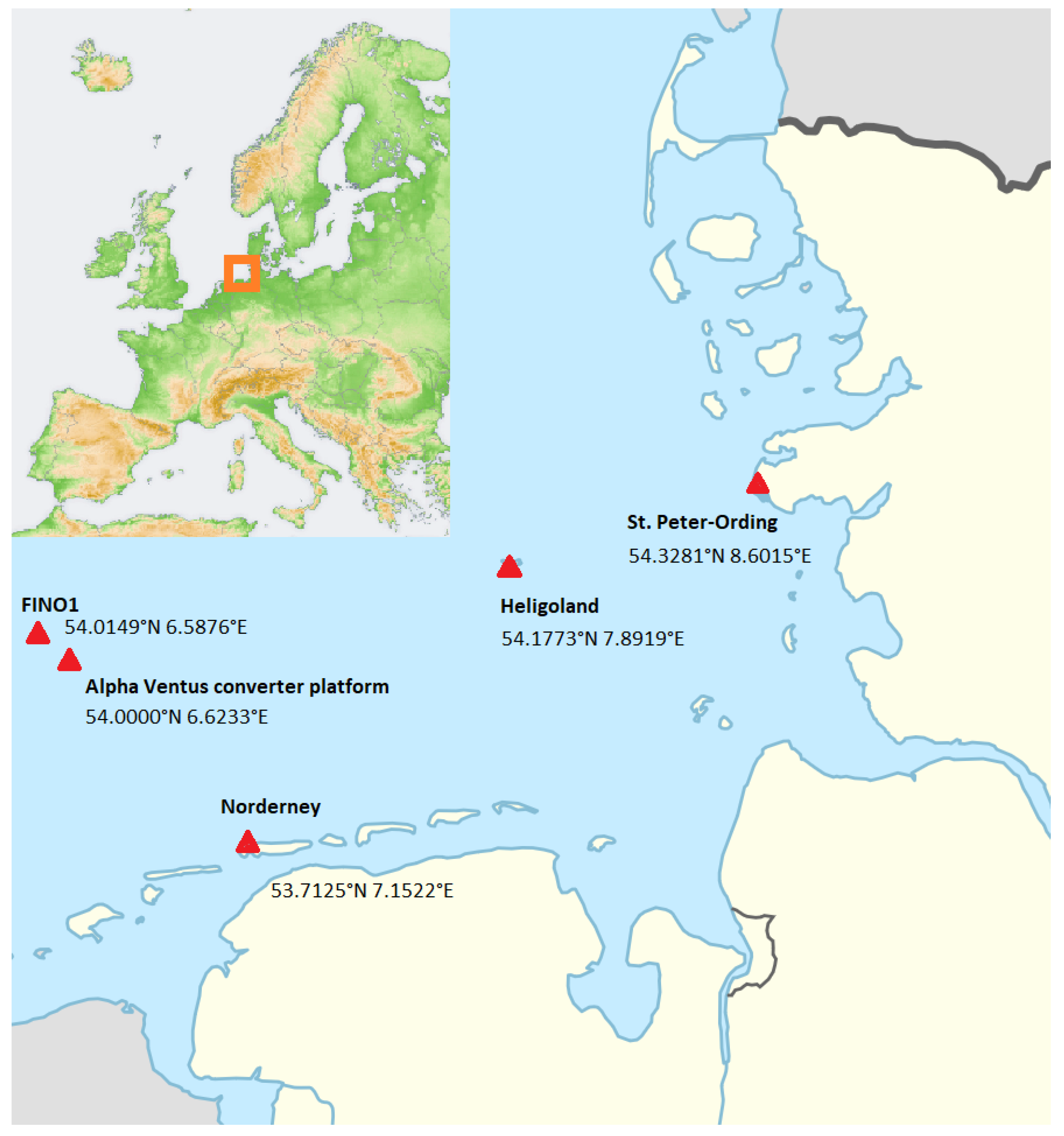
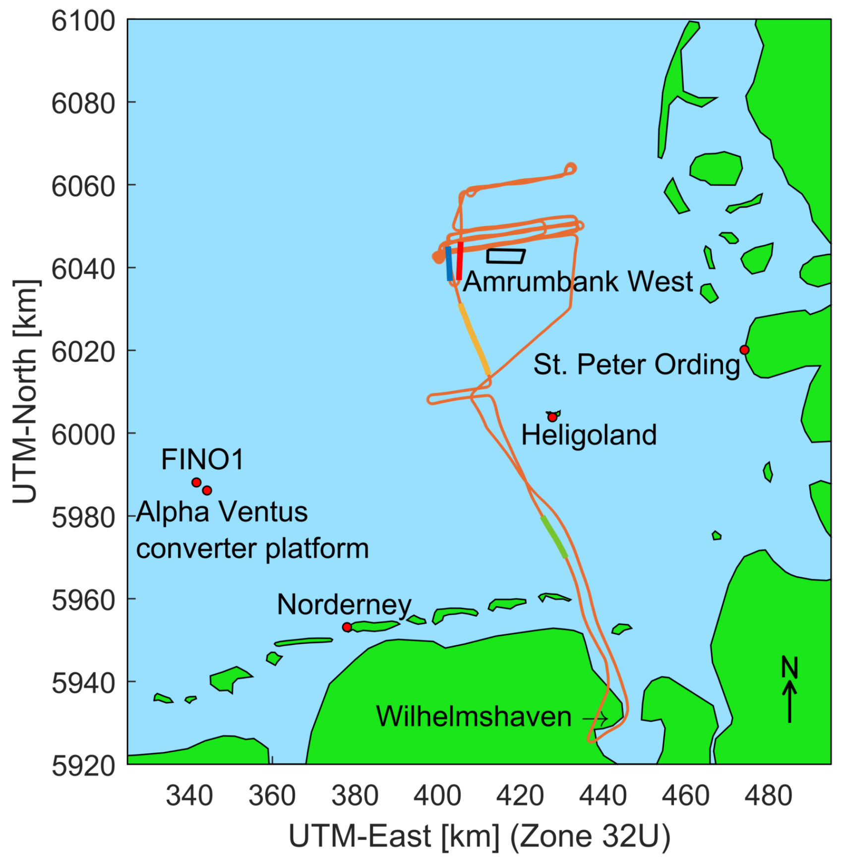
3. Study Sites and Data Base
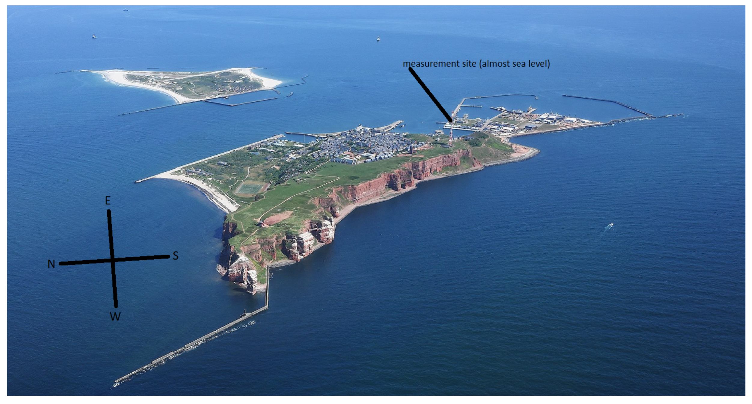
The data sets for this study were recorded using ground-based pulsed Doppler wind lidar systems of the types WindCube WLS8-8, WindCube v1, and WindCube v2, developed and manufactured by the former French company Leosphere (now Vaisala). The pulsed laser infers the horizontal wind speed from so-called line-of-sight (LOS) or radial wind speeds V r using a four-Doppler-beam-swing (DBS) scan [54,55]. An internal optical switch steers the laser beam at four azimuth angles in successive intervals of 90 (i.e., 0 , 90 , 180 , and 270 ) to form a conical scan with a fixed elevation angle with respect to the horizontal. The LOS or radial speed is then inferred within a range gate of 40 m from the Doppler shift of the resulting return signal due to atmospheric particle scattering with respect to the original signal. The pulsed system together with the internal algorithm enables the simultaneous reconstruction of the mean wind speed and wind direction from several heights or range gates. The measurement quality is evaluated according to a threshold based on the carrier-to-noise ratio (CNR), which is dependent upon atmospheric conditions, such as the aerosol backscatter, turbulence, humidity, and precipitation. Values with a CNR of less than 22 dB are discarded. Furthermore, events with rain periods are discarded. Only lidar data with availability of 80% for each 10 min value are used.
The wind lidar systems were installed consecutively at different locations of the German Bight (Figure 1), the WindCube v1/v2 at FINO1, the Alpha-Ventus offshore wind park, and St. Peter-Ording, the Windcube WLS8-8 at Heligoland and Norderney. Only data averaged over 10 min were used for this study.
The WindCube WLS8-8 system obtained data on wind speed and wind direction at 25 altitudes (40 m to 500 m, with a vertical resolution of 10 m up to 100 m, 20 m up to 400 m, and 50 m up to 500 m) for the locations Heligoland and Norderney.
The WindCube v1/v2 were operated at different sites: a WindCube v2 (measurement altitudes from 71 m to 241 m with a vertical resolution of 20 m) at the FINO1 research platform; a WindCube v1 (measurement altitudes 71 m, 81 m, 91 m, 102 m, 119 m, 139 m, 159 m, 179 m, 199 m, 249 m, 279 m, 319 m) at the substation of the Alpha-Ventus wind farm; a WindCube v2 (measurement altitudes 71 m, 81 m, 91 m, 102 m, 119 m, 139 m, 159 m, 179 m, 199 m, 249 m, 279 m, 300 m) at St. Peter Ording. All lidar systems were installed and monitored under remote surveillance by the company UL International GmbH, Germany. An overview of the operation times at the different locations is provided in Table 1.

3.1. Heligoland

The WLS8-8 system was located at the island Heligoland at the site of the Alfred Wegener Institute, Helmholtz Centre for Polar and Marine Research and almost at sea level (2 m) from 24 March 2017 to 23 March 2018. The data availability, defined as the percentage of wind profiles where at least half of the data points of the wind profiles were valid, was 98.5%. Since no wind farms are in close proximity to the island, only the orography of the island itself alters the wind field. The island is elevated up to 60 m with 50 m high cliffs in the north (Figure 2). The smaller island “Düne” is located to the northeast of the lidar. This limits the unobstructed wind sector to 90° to 270°, neglecting the flat and narrow southern part of the island. The site will be referred to as HL.

3.2. Norderney

At Norderney, the wind lidar was installed at the measurement site of the German Weather Service (DWD) from 9 August 2019 to 8 August 2020. The data availability, defined as the percentage of wind profiles where at least half of the data points of the wind profiles were valid, was 80%. The site will be referred to as NO.
Routine automated radiosondes are launched twice per day by DWD. To compare the different measurement periods for the one-year data sets at Heligoland and Norderney, radiosonde measurements up to 500 m altitude are analysed for the LLJ occurrence for both time periods. Besides wind data, information on temperature and humidity is available from the soundings.

3.3. FINO1/Alpha-Ventus

The research platform FINO1 was constructed in 2003 to investigate, among other parameters, wind and wave fields in the North Sea. The platform is located approximately 45 km north of the German island Borkum. At the time of the measurements (2017–2018), FINO1 was surrounded by the wind farms Alpha-Ventus to the east, Borkum Riffgrund 1 and 2 to the south, and Trianel Windpark Borkum 1 to the west. The wind farm Merkur which is located next to FINO1 to its west and north was under construction in 2017. Due to the installed wind farms, FINO1 has only a small sector of open wind field to the north-northwest which is, however, facing away from the coast.
A Windcube v2 lidar was installed on the platform FINO1, located 24 m above sea level from 1 April 2017 to 31 March 2018. Another Windcube v2 lidar was installed at the electrical substation of the wind farm Alpha-Ventus. The transformer station is located southeast of the wind farm and thus in the immediate vicinity of FINO1. The wind farms Borkum Riffgrund 2 (south), Borkum Riffgrund 1 (southeast), Trianel Windpark Borkum 1 (west) and Alpha-Ventus (west to north) surround the measuring station mostly. The wind farm Nordsee One at the east-southeast of the measurement point was under construction from December 2015 to September 2017. Individual wind turbines were tested since December 2017, and the complete wind farm started operation in December 2017. In conclusion, this means that only the sectors of 0° to 60° and 135° to 180° are facing an open wind field. Both platforms are 24 m and 29 m above mean sea level (MSL), respectively. The sites will be referred to as FI/AV, respectively.

3.4. St. Peter-Ording

Another WindCube v2 lidar system was installed at the coast at St. Peter-Ording, Germany, for a short measurement campaign from 23 May 2017 to 19 June 2017. The lidar was located approximately 1 km away from the shore with only a flat beach obstructing the way. Thus the open wind field ranges from 180° to 330°. The system was located at 10 m above MSL. The site will be referred to as SPO.

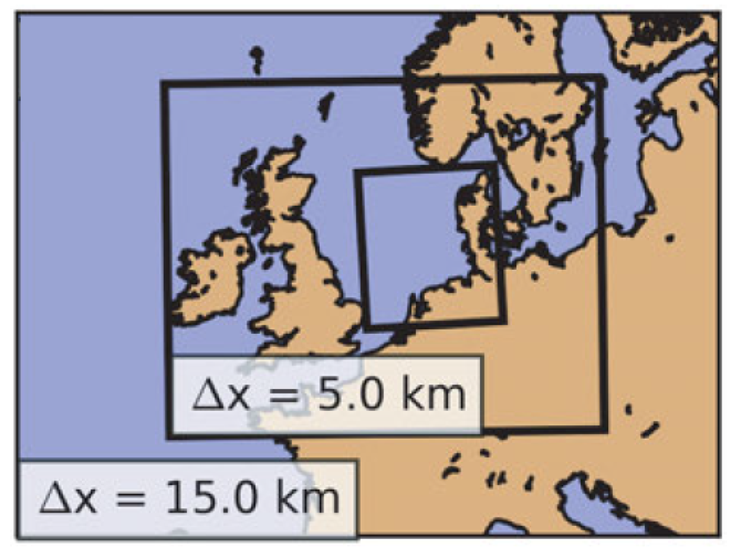
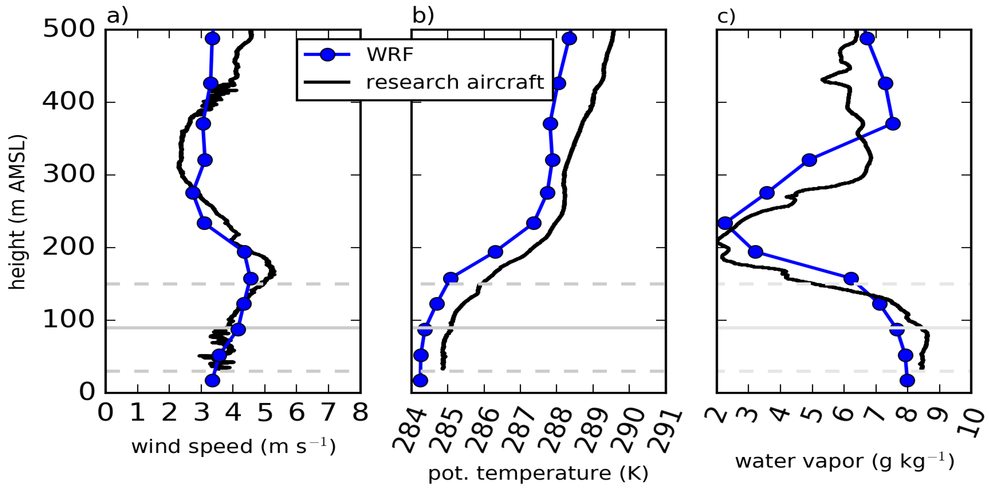
4. WRF Modelling of the LLJ

In the framework of the project WIPAFF [4], airborne in situ meteorological measurements were performed with the research aircraft Dornier 128 above the German Bight [53]. During the flight on 2 June 2017, a low-level jet was measured in parallel with the wind lidar systems. For this particular day, simulations with the weather research and forecasting (WRF, 3.8.1) model were performed to validate the model performance in the case of an LLJ and to complement the lidar and airborne measurements for studying the horizontal extent of the phenomenon. The full details of the numerical setup are described in [57]. However, the effect of wind farms is not parameterized here, as the focus is the evolution of LLJs. The model has three domains with horizontal grid sizes of 15 km, 5 km, and 1.6 km, respectively (Figure 3). All domains have the same vertical levels, below 200 m the spacing of the vertical levels is 35 m, whereby the lowest full level is located approximately 20 m above MSL. The initial and lateral boundary conditions are defined by operational ECMWF (European Centre for Medium-Range Weather Forecasts) analysis data, having a horizontal grid size similar to the outermost domain. The model is initialized at 12:00 UTC on 1 June 2016, resulting in 18 h spin-up time. The model uses the following parameterizations in all three domains: the WRF double-moment six-class cloud microphysics scheme (WDMS [58]), the rapid radiation transfer model for GCM (RRTMG) scheme for short- and longwave radiation [59], the Noah land surface model [60] and the Mellor–Yamada–Nakanishi–Niino (MYNN) boundary layer parameterization [61] with a modified mixing length in the free atmosphere [62]. The outermost domain uses a cumulus parameterization [63], whereby the two innermost domains have a convective allowing grid size.

5. Results and Discussion

This section consists of different subsections: In Section 5.1, the general wind conditions (Weibull distribution, wind roses) at the sites Heligoland and Norderney are presented. For estimating the wind resource for a specific site of wind turbine operation, normally wind statistics covering an entire year are used. Therefore we provide the following analyses for the temporal base of one year. Then statistics of the low-level jet for the two sites are compared in Section 5.2. Section 5.3 investigates the relation between LLJ and stability. Section 5.4 presents a case study of the horizontal extent of an LLJ based on several wind lidar systems distributed within the German Bight, additional airborne in situ measurements and numerical simulations.

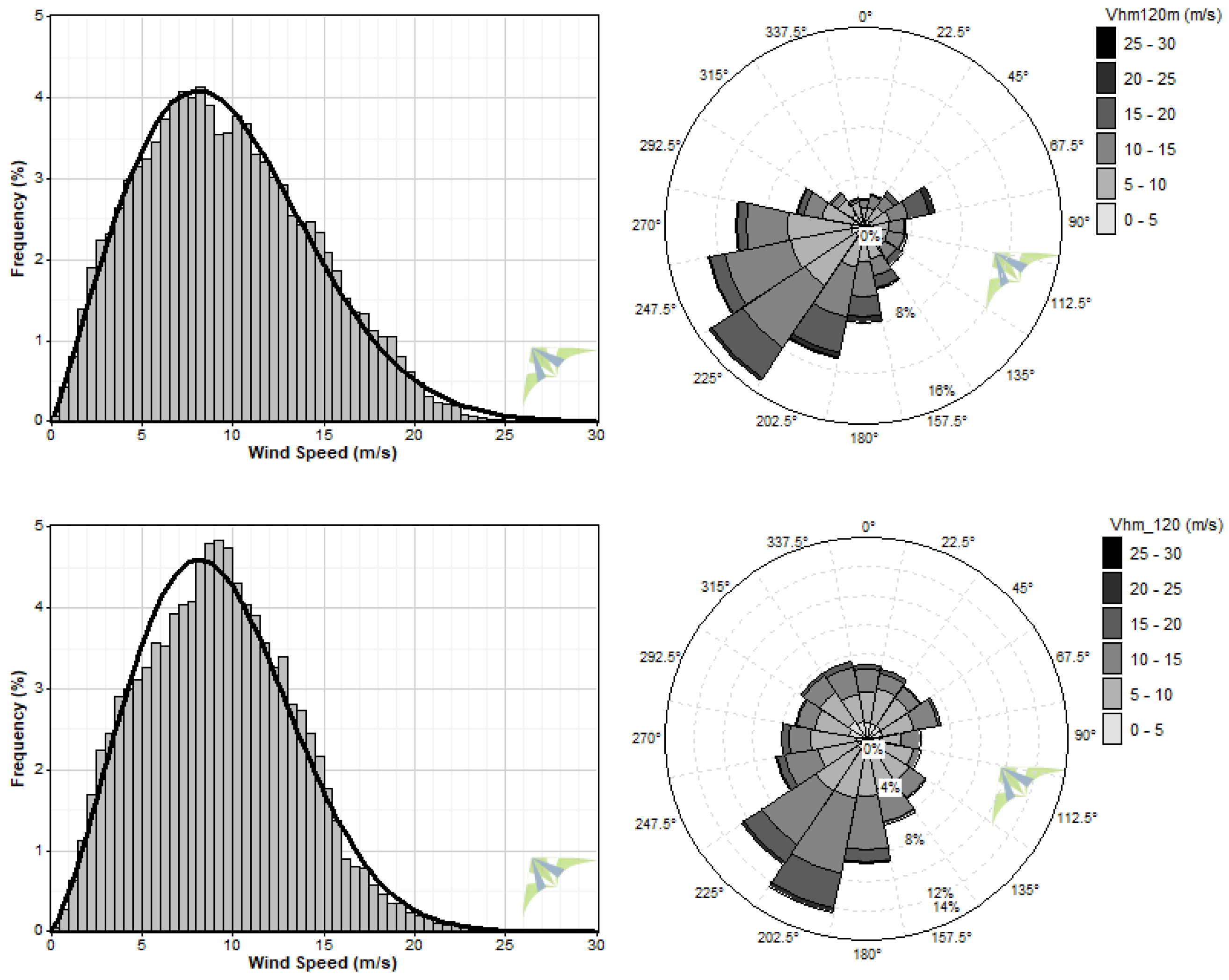
5.1. Weibull Distribution and Wind Roses for the Sites Heligoland and Norderney

The Weibull wind speed distributions at Heligoland and Norderney (Figure 4), at a representative hub height (120 m), are similar: The scale factor, which is proportional to the most likely wind speed, is A = 10.91 m s 1 for Heligoland and 10.39 m s 1 for Norderney. This is in agreement with typical long-term values in the North Sea obtained at FINO1 [33]. The shape factor is k = 2.12 for Heligoland and 2.33 for Norderney, which are typical values for the German Bight [33]. The wind roses are similar as well. However, the most frequent wind direction for Heligoland was SW, and for Norderney SSW. Note that the data were obtained during different years. Therefore, the differences may be attributed to generally different prevailing wind conditions in the different years, or to systematic differences due to different locations.

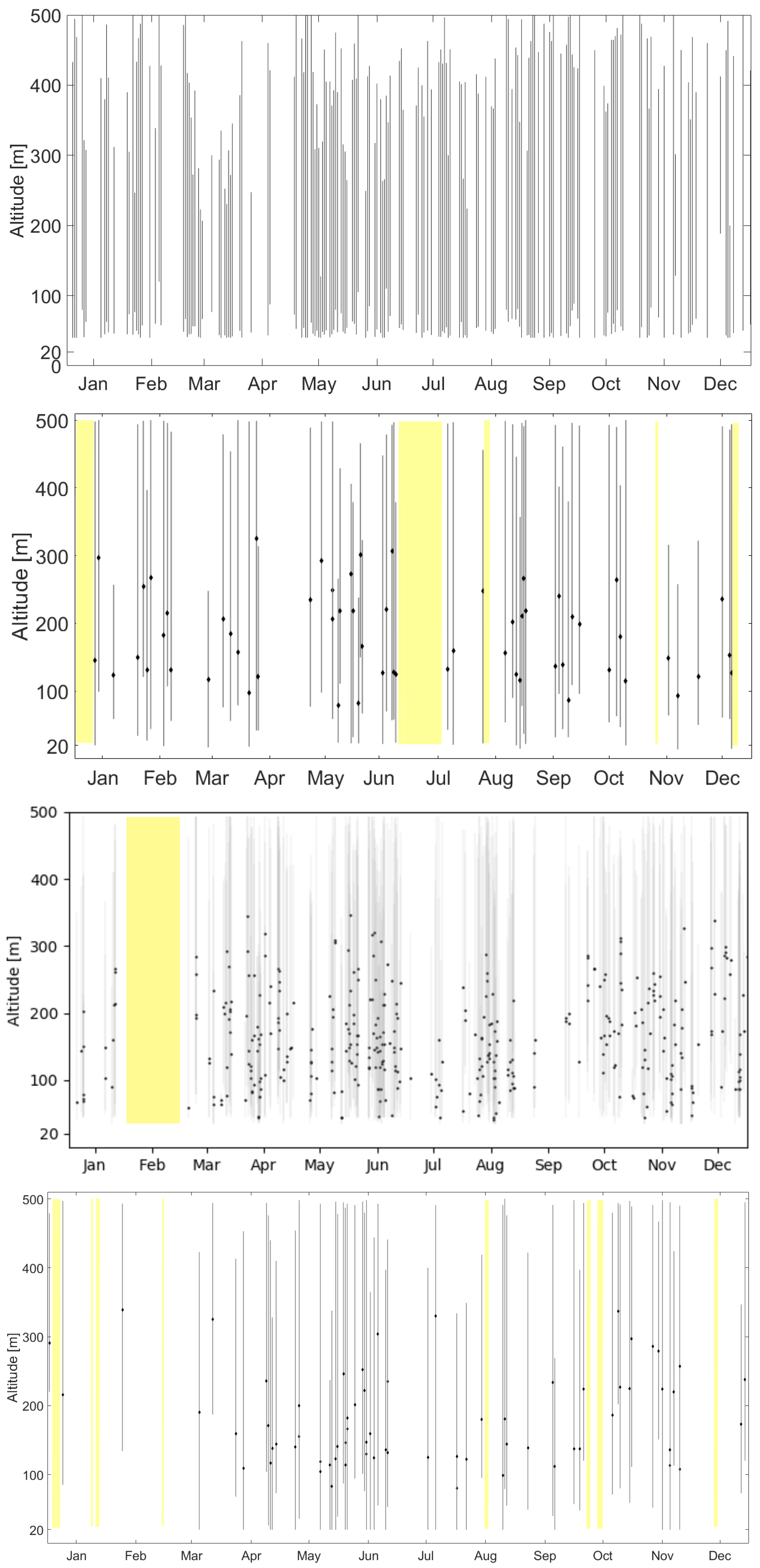
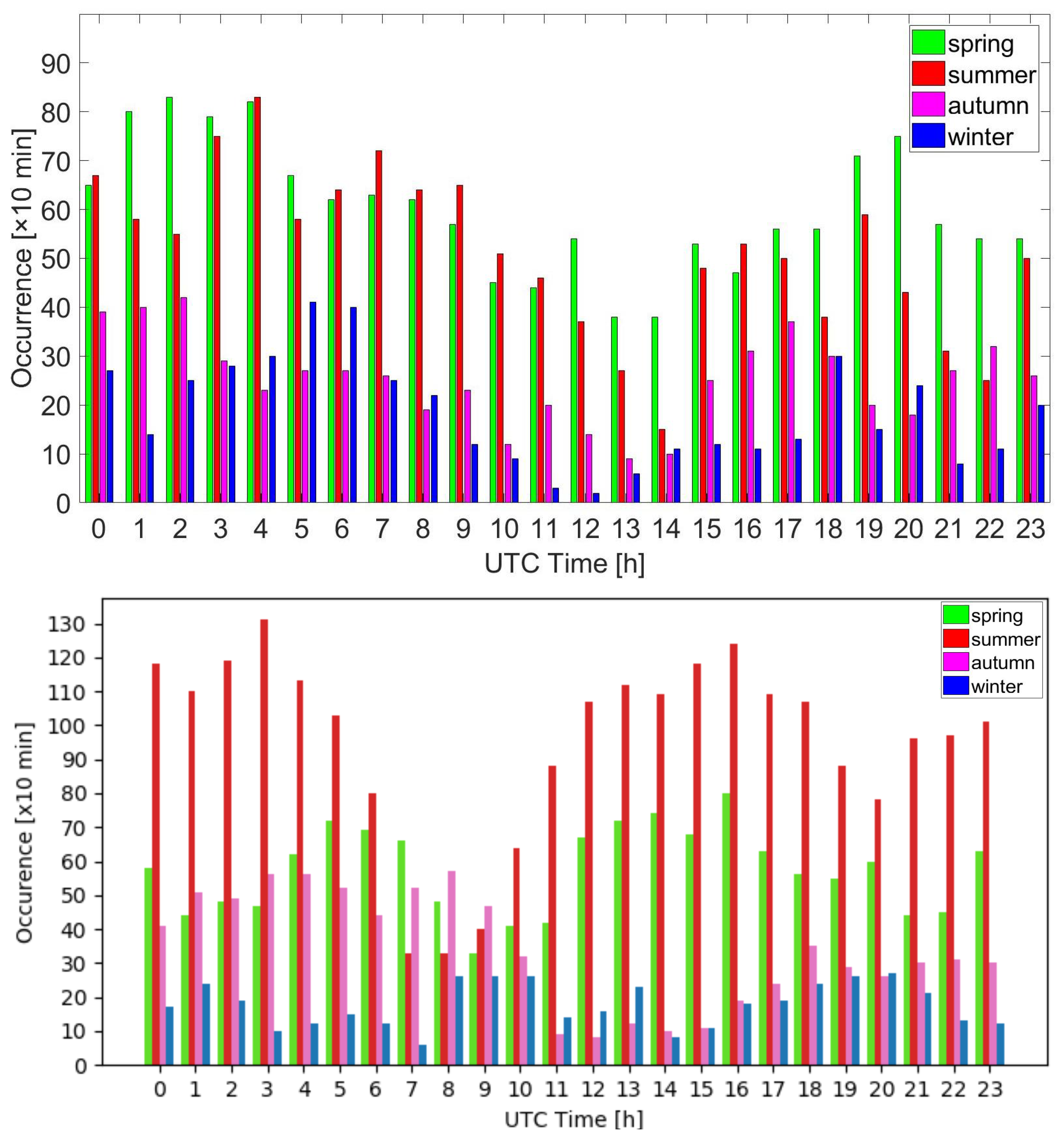
5.2. Statistics on LLJ Occurrence

For the site Heligoland, the data set of a full year from 24 March 2017 to 23 March 2018 is analysed here. LLJ profiles were recorded during 7.19% of the total time.
For the site Norderney, the data set from 9 August 2019 to 8 August 2020 is analysed. LLJ profiles were recorded during 11.13% of the total time.
Figure 5 shows the occurrence of LLJ events throughout the year based on lidar data, and for comparison also based on radiosonde data obtained in the same time period (only available at Norderney). For each day where an LLJ occurred, the altitude interval affected by the LLJ is marked by a vertical black line. This indicates the altitude with the upper boundary of the minimum wind speed and the lower boundary where the wind speed has the same value as the altitude of the minimum wind speed. It can be seen that for both sites, the distribution of LLJ events follows specific patterns of typically a few consecutive days. This is in agreement with the typical lifetime of synoptic circulation patterns which either enable or prevent the formation of LLJ by different atmospheric conditions [10] and was also observed in the one-year data set of Braunschweig, Northern Germany [27]. For both sites, most LLJs appeared in spring (March, April, May) and summer (June, July, August), with fewer in autumn (September, October, November) and even less in the winter months (December, January, February).
The LLJ profiles identified by the radiosondes at 0 and 12 UTC at the site Norderney are provided in Figure 5 for the same time periods as the wind lidar observations. A similar annual distribution is observed by the continuous wind lidar data from the same site. The annual LLJ distribution is comparable for both time periods.
Figure 6 shows the distribution of LLJ events over the day for Heligoland and Norderney. A minimum occurrence is visible between 9 and 14 UTC. LLJs occur most frequently during the nighttime. The diurnal distribution is similar for Norderney with a minimum LLJ occurrence between 10 and 14 UTC.
The jet core height distribution of the LLJ maximum for Heligoland is located most frequently at an altitude of 120 m, thus within the altitude of the rotor blades. LLJ core heights have been identified between 40 m and 250 m in 86% of all cases. For Norderney, the altitude distribution is similar with the most frequent occurrence at an altitude of 110 m. The distribution of the maximum wind speed is similar for both cases as well. The maximum LLJ wind speed typically increases with core height. This feature has been observed for the radiosonde and continuous lidar data both at Heligoland and Norderney (not shown). This relationship has also been shown in [64].

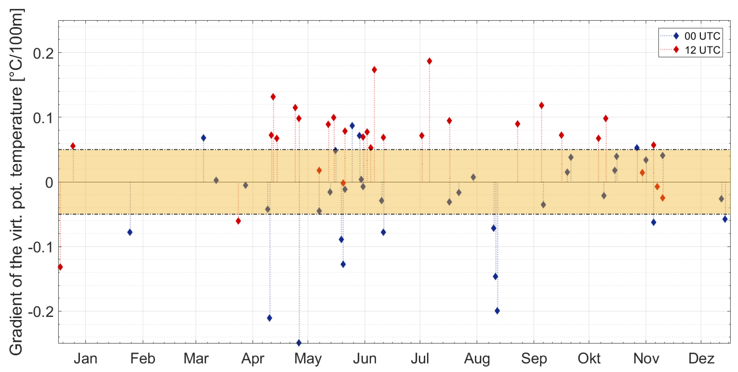
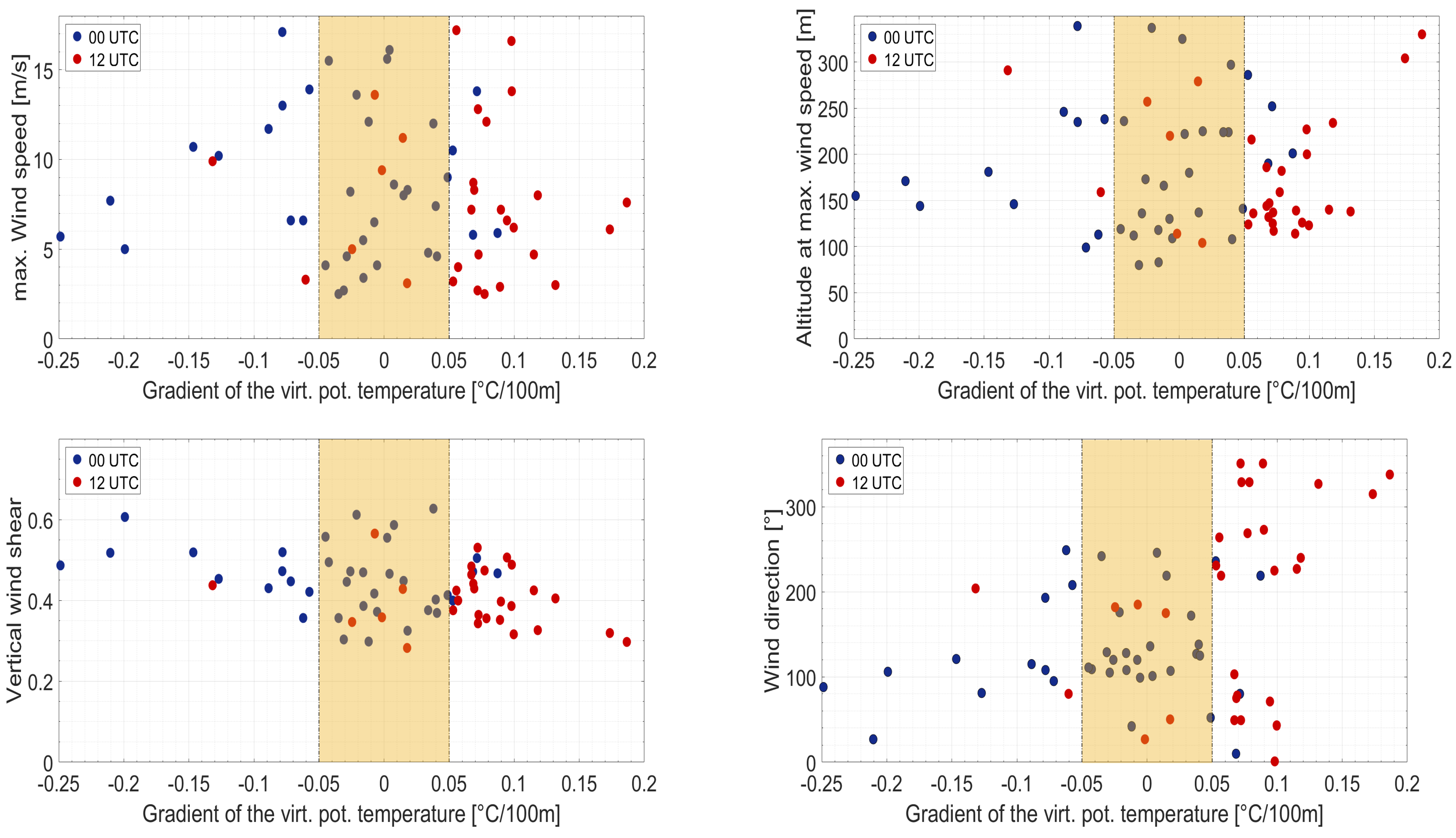
5.3. LLJ Dependence on Atmospheric Stability

For the radiosonde data set, temperature and humidity data are available as well. Figure 7 shows the vertical gradient of the virtual potential temperature, which is an indicator of atmospheric stability, for the individual LLJ events. There is a trend that LLJ events observed around noon occurred mostly during stable conditions. At midnight, LLJ events are observed most frequently for neutral or even unstable atmospheric conditions.
The LLJ parameters’ relation to stability and others is investigated more in detail in Figure 8: The LLJ maximum wind speed varies between 2.5 and 17 m s 1 , with no clear dependence on stability. The LLJ core height varies between 70 and 350 m without a clear correlation with stability.
Vertical wind shear is confined to the range of 0.3 to 0.6. This is significantly higher than previously reported values for coastal zones, e.g., a vertical wind shear coefficient of 0.11 was reported for neutral conditions for platforms in the Gulf of Mexico [65]. The impact of wind shear in the range of 0.1 to 0.4 on the probability of operation for wind turbines for a fixed Weibull distribution near the surface was investigated in [66]: A higher wind shear results in a higher probability of operation of wind turbines, in particular for turbines with high cut-in speed.
The wind direction for neutral and unstable conditions is most frequently from north to east during the night. This can be explained by colder air masses above land which are advected to the warmer sea surface.
During the daytime, stable conditions are observed in all wind directions. This is as expected for wind directions from the sector east to southwest if synoptic-scale flow dominates over local effects like sea breeze, as warmer air masses from land are transported above the colder water surface, leading to a surface-based temperature inversion. For wind from the sector west to northeast, this is unexpected. However, one has to take into account that for these wind directions, the radiosondes are transported from the island of Norderney towards the coast, where warmer temperatures are likely. The distance of the radiosondes from the launch site up to reaching an altitude of 500 m was typically within the radius of 3 km.

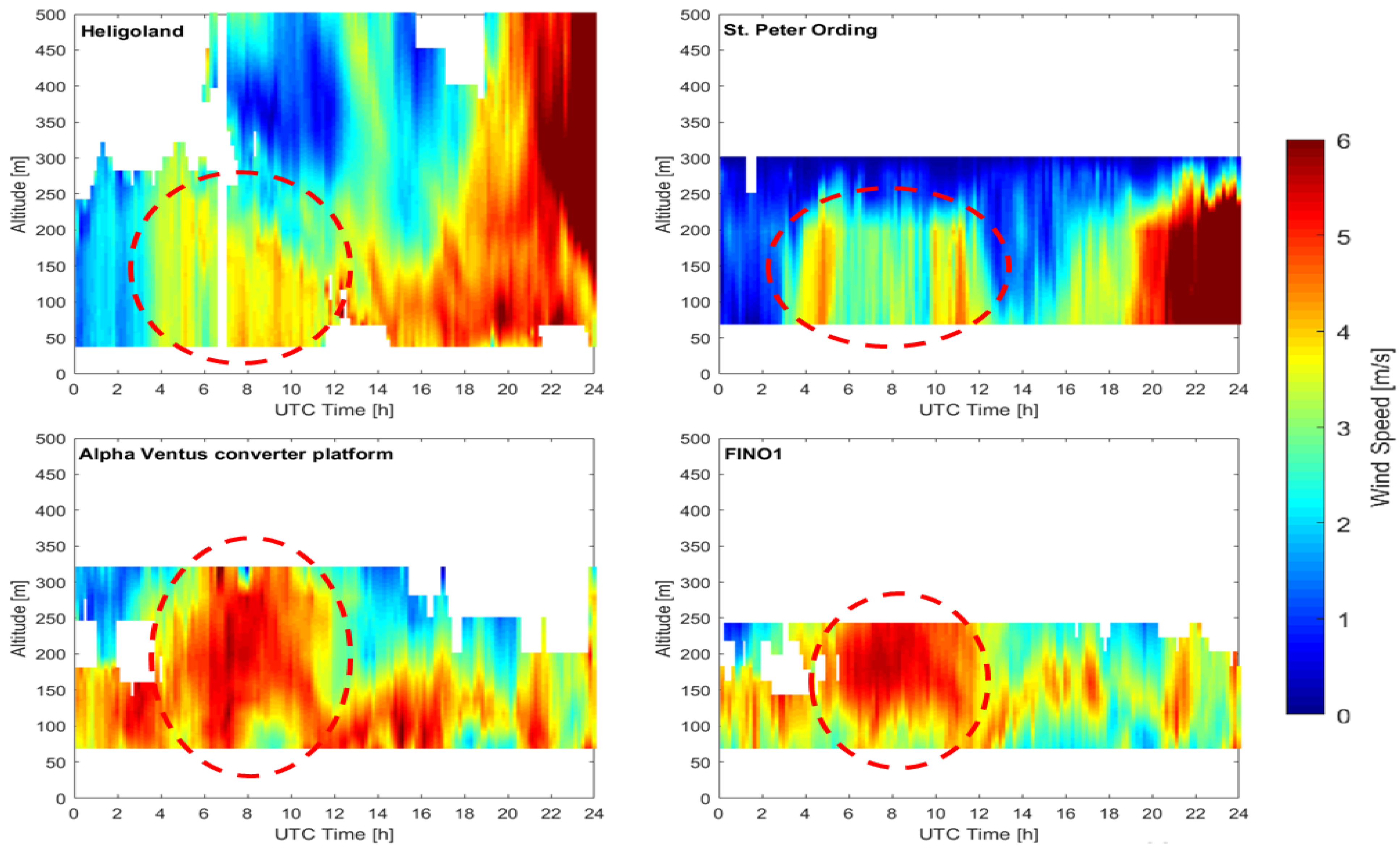
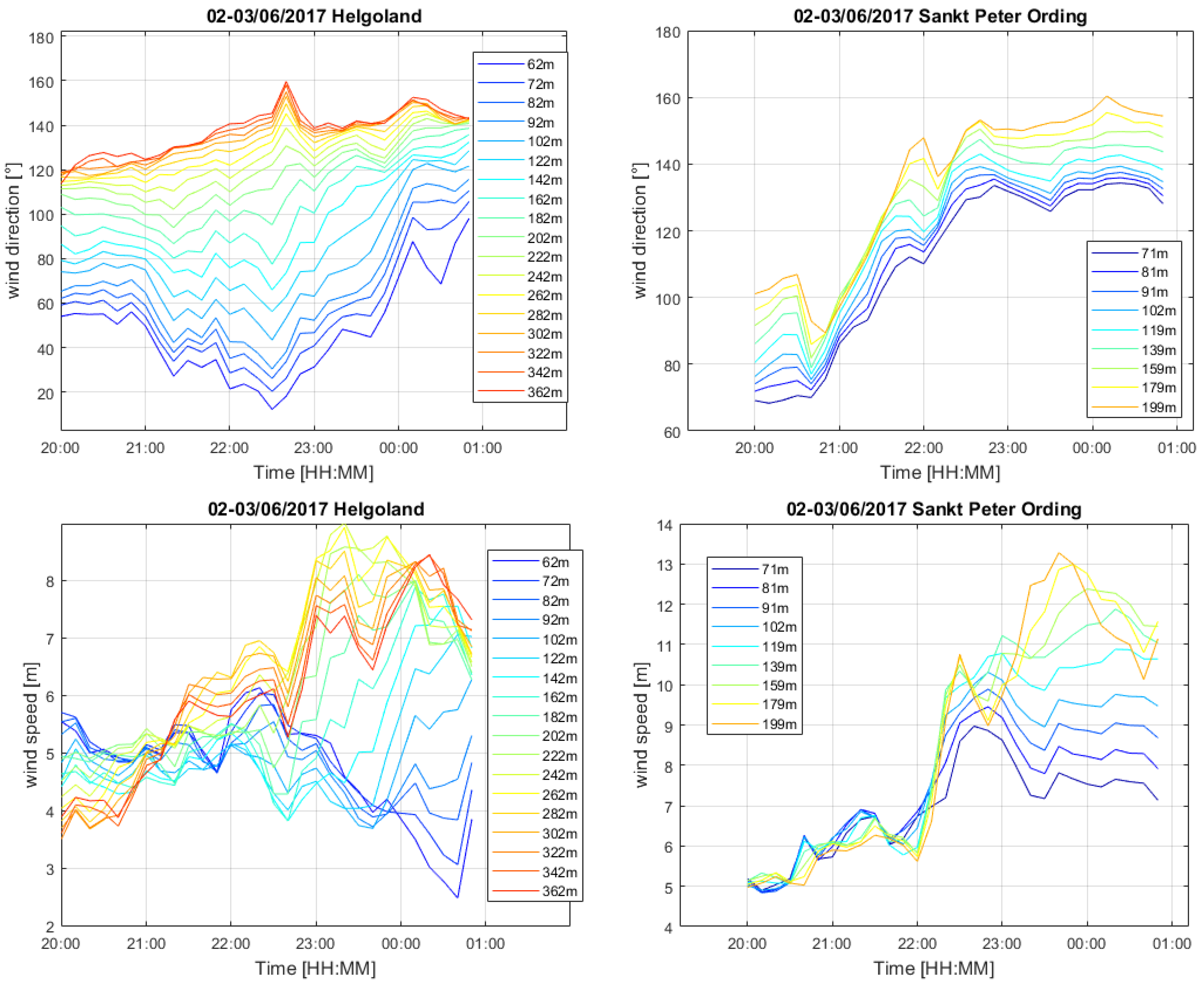
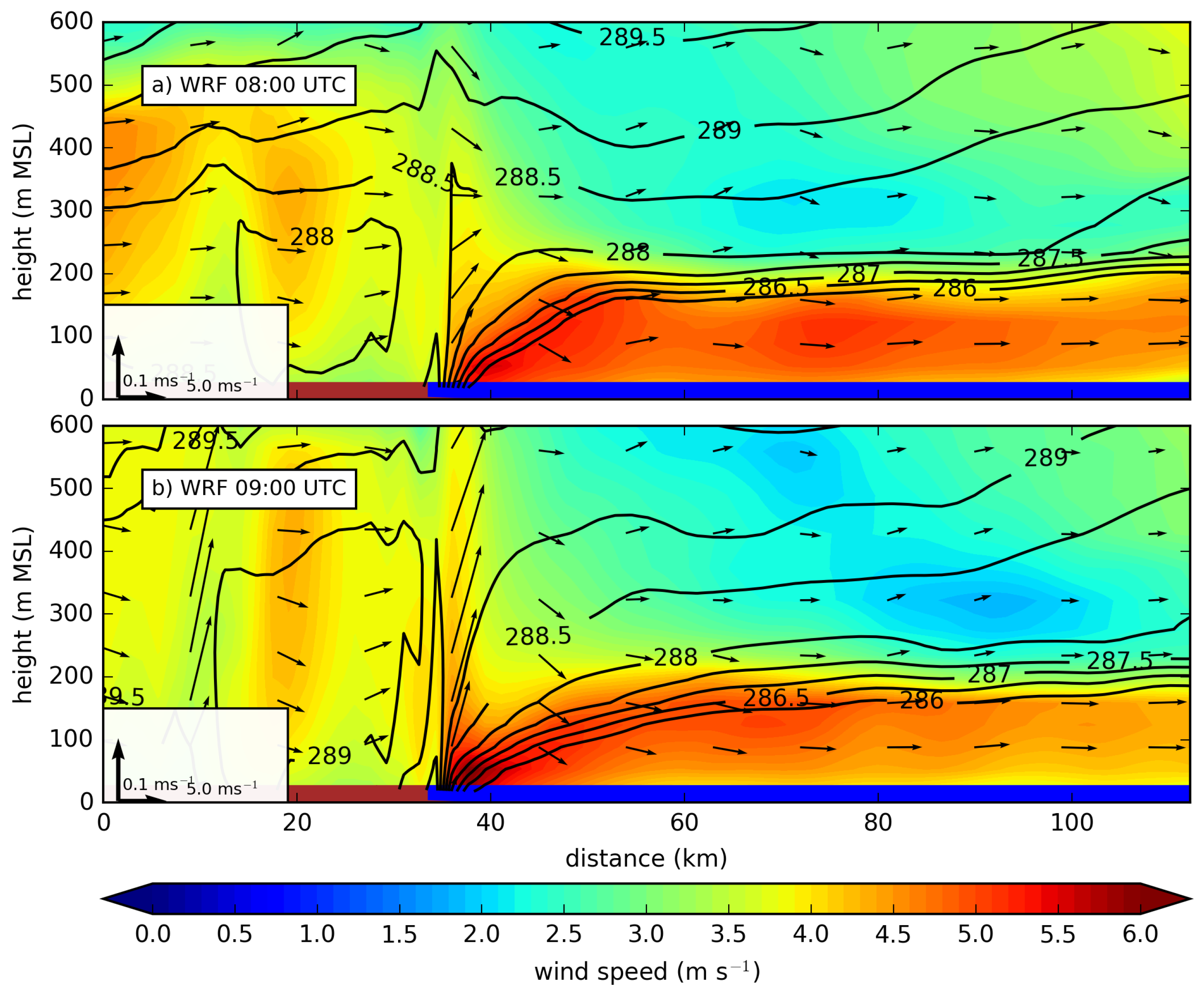
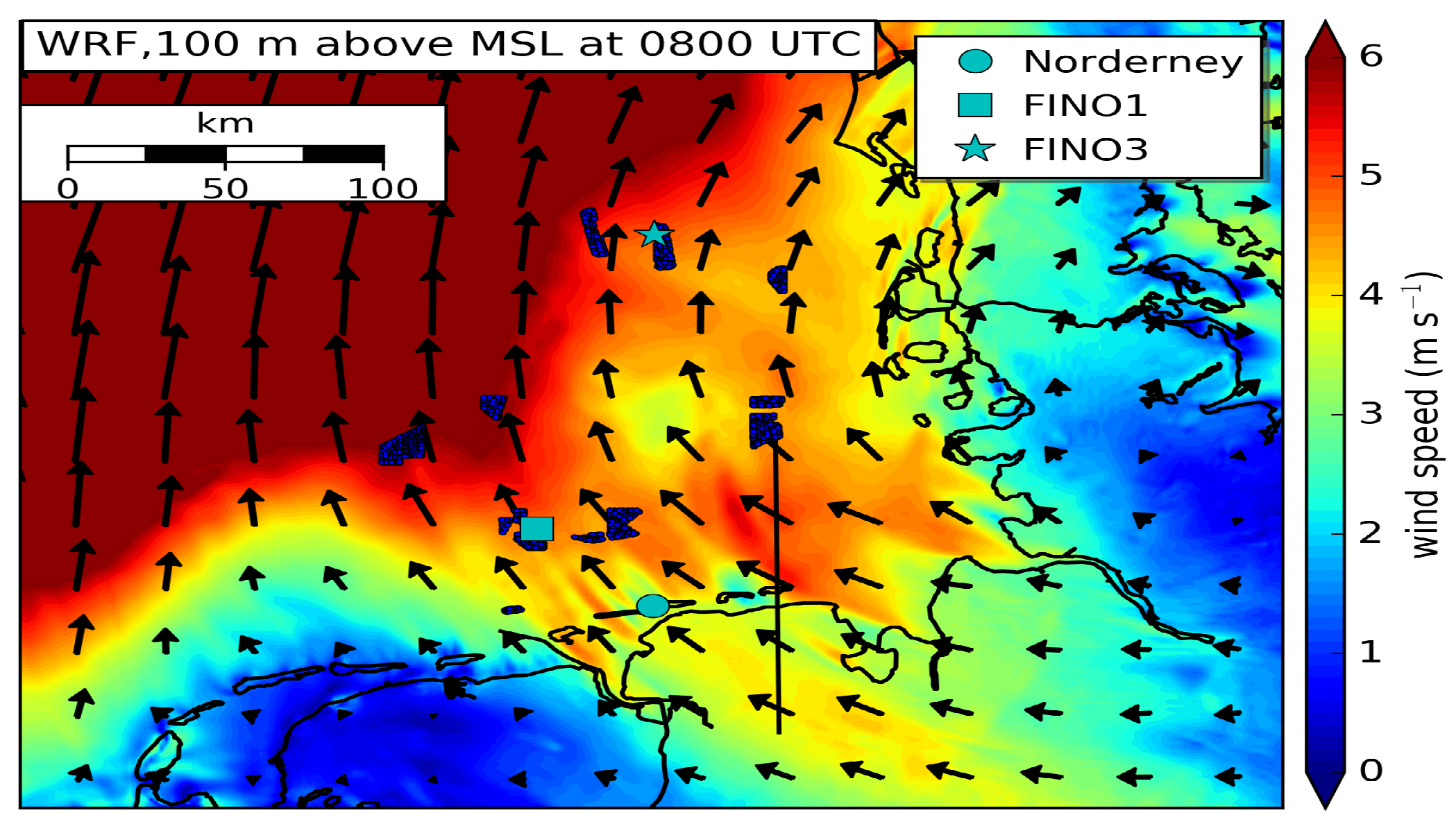
5.4. LLJ Extent: Case Study for 2 June 2017

On 2 June 2017, a day with southeasterly wind directions, water temperatures from 12 °C in the central German Bight up to 17 °C along the coastline, and air temperatures from 13 °C in the central German Bight up to 16 °C over land in northwestern Germany, an LLJ event was observed by four wind lidar systems and airborne measurements near the wind park Amrumbank West simultaneously (Figure 9). Figure 10 additionally shows profiles of a nocturnal LLJ which was established later that day at the locations Heligoland and St. Peter-Ording.
An interplay of several mechanisms is responsible for the observed acceleration of wind speed below 300 m. The advection of relatively warm air that has been heated up on its way above the warmer land surface over the cold North Sea and relatively cold near-surface air resulted in surface-based temperature inversion with cold air masses below and warmer air masses above, which constitutes a stably stratified atmosphere. As known from the nocturnal LLJ, a temperature inversion decouples friction forces and supports the development of an LLJ. Additionally, the transition between land to open sea is associated with a dramatic change in surface roughness, resulting in low surface friction forces over the open water causing higher wind speeds. In contrast, the warm land and the cold ocean would expect a sea-breeze circulation that counteracts the observed wind direction.
A deeper look into the spatial extent of the LLJ is provided by the use of WRF simulations.
WRF simulations were able to reproduce airborne measurements by a Dornier-128 research aircraft [52,53] (Figure 11) of a stable stratification above land during the morning, which is persistent above the sea surface at 09:15 UTC (Figure 12). Associated with the temperature inversion, a belt of increased wind speed is represented during the time of the observations, confirming the different wind speed observations (Figure 12). The vertical cross section aligned in the north–south direction shows the increase of wind speed corresponding to the height of the temperature inversion (Figure 13).
Therefore, the overall extent of the LLJ above the German Bight can be estimated as at least 110 km in the north–south direction (from Wilhelmshaven to Amrumbank West) and 130 km in the east–west direction (from St. Peter-Ording to FINO1) from observational data. This is in agreement with observations above land, where LLJs can extend several hundreds of kilometres in length and width [67]. WRF simulations even suggest a larger extent of up to 170 km in the north–south direction and of at least 260 km in the east–west direction (see wind speed at 100 m altitude in Figure 13).

6. Conclusions

LLJs occur frequently at the coast of the North Sea, with a maximum occurrence in spring and summer and during the night. As stable stratifications decouple friction force from the air above and lead to an acceleration of wind speed in the form of an LLJ, the frequent observations of LLJ events are in agreement with the observations that stable stratifications above the North Sea are present frequently, around one-third of the year. As both spatial and temporal variability of the LLJ are significant, wind profile measurements in the direct vicinity of the wind park are necessary to improve the representation of the effect. At Heligoland, an LLJ occurred on 42.5% of all days for an entire year during all seasons, with most events in spring and summer. This is in agreement with the observations that stable stratifications above the North Sea are present around one-third of the year [34]. With the extent exceeding 100 km in longitudinal and latitudinal directions, several wind parks can be affected by LLJs. WRF simulations were capable of reproducing the LLJ in the wind profile at the time and location of the airborne observations, and therefore constitute a suitable tool for investigating this particular wind phenomenon. Further, they were used to estimate the extent of the LLJ in the German Bight.

Author Contributions

T.R. and A.L. wrote the manuscript; O.H., T.S., Y.B.T., T.R. and B.C. analysed the lidar data; B.C. and T.N. operated the lidar systems; S.S. performed the numerical simulations. All authors commented and contributed to the text. All authors have read and agreed to the published version of the manuscript.

Funding

The airborne and lidar observations have been funded by the project WIPAFF of the German Federal Ministry for Economic Affairs and Climate Action under grant number 0325783B. The Heligoland lidar observations have been partly funded by the project AVATAR, German Federal Ministry for Economic Affairs and Climate Action, grant number 20Y1501F. Ongoing lidar measurements and their analysis is funded by the project X-Wakes, German Federal Ministry for Economic Affairs and Climate Action, grant number 03EE3008B. We acknowledge support by the Open Access Publication Funds of Technische Universität Braunschweig.

Data Availability Statement

Lidar data of the Heligoland site are publicly available at PANGAEA [68]. Lidar data of the Norderney site will be published at PANGAEA in the same way at the end of the X-Wakes project. The radiosonde data sets are available at http://opendata.dwd.de/climate_environment/CDC/observations_germany/, accessed on 1 April 2022. The airborne data are available at PANGAEA [52].

Acknowledgments

The wind lidar data have been analysed during many student projects. In particular, the authors would like to thank Jutta Meier, Sven Rübberdt, Johannes Degenhardt, and Pascal Brudke for their analyses during their diploma, bachelor, and master theses. The authors would like to thank the aircraft crew Rudolf Hankers, Thomas Feuerle, Mark Bitter, and Helmut Schulz for the successful airborne measurements. The installation and remote supervision of the Heligoland wind lidar have been performed by Christian Krüger of UL International. The authors would like to thank Heino Peters, Andreas Schmidt, Helgo Denker, Eva-Maria Brodte, and Karen Wiltshire for the opportunity to install the wind lidar at Heligoland at the facilities of the Alfred Wegener Institute Helmholtz Centre for Polar and Marine Research, and the German Weather Service for providing access to the study site at Norderney. The authors would like to thank Stefan Emeis for involving us in the project WIPAFF.

Conflicts of Interest

The authors declare no conflict of interest.

References

  1. Arbeitsgruppe Erneuerbare Energien—Statistik (AGEE-Stat): Zeitreihen zur Entwicklung der Erneuerbaren Energien in Deutschland, Stand Februar. Available online: https://www.erneuerbare-energien.de/EE/Navigation/DE/Service/Erneuerbare_Energien_in_Zahlen/Zeitreihen/zeitreihen.html (accessed on 1 April 2022).
  2. Steele, C.J.; Dorling, S.R.; von Glasow, R.; Bacon, J. Modelling sea-breeze climatologies and interactions on coasts in the southern North Sea: Implications for offshore wind energy. Q. J. R. Meteorol. Soc. 2015, 141, 1821–1835. [Google Scholar] [CrossRef] [Green Version]
  3. Schulz-Stellenfleth, J.; Emeis, S.; Dörenkämper, M.; Bange, J.; Cañadillas, B.; Neumann, T.; Schneemann, J.; Weber, I.; zum Berge, K.; Platis, A.; et al. Coastal impacts on offshore wind farms—A review focussing on the German Bight area. Meteorol. Z. 2002. [Google Scholar] [CrossRef]
  4. Platis, A.; Bange, J.; Bärfuss, K.; Cañadillas, B.; Hundhausen, M.; Djath, B.; Lampert, A.; Schulz-Stellenfleth, J.; Siedersleben, S.; Neumann, T.; et al. Long-range modifications of the wind field by offshore wind parks – results of the project WIPAFF. Meteorol. Z. 2020, 29, 355–376. [Google Scholar] [CrossRef]
  5. Cañadillas, B.; Foreman, R.; Barth, V.; Siedersleben, S.; Lampert, A.; Platis, A.; Djath, B.; Schulz-Stellenfleth, J.; Bange, J.; Emeis, S.; et al. Offshore wind farm wake recovery: Airborne measurements and its representation in engineering models. Wind. Energy 2020, 23, 1249–1265. [Google Scholar] [CrossRef]
  6. Schneemann, J.; Rott, A.; Dörenkämper, M.; Steinfeld, G.; Kühn, M. Cluster wakes impact on a far-distant offshore wind farm’s power. Wind. Energy Sci. 2020, 5, 29–49. [Google Scholar] [CrossRef] [Green Version]
  7. Nygaard, N.G.; Steen, S.T.; Poulsen, L.; Pedersen, J.G. Modelling cluster wakes and wind farm blockage. J. Phys. Conf. Ser. 2020, 1618, 062072. [Google Scholar] [CrossRef]
  8. Wagner, D.; Steinfeld, G.; Witha, B.; Wurps, H.; Reuder, J. Low Level Jets over the Southern North Sea. Meteorol. Z. 2019, 28, 389–415. [Google Scholar] [CrossRef]
  9. Blackadar, A.K. Boundary layer wind maxima and their significance for the growth of nocturnal inversions. Bull. Am. Met. Soc. 1957, 38, 283–290. [Google Scholar] [CrossRef] [Green Version]
  10. Emeis, S. Wind speed and shear associated with low-level jets over Northern Germany. Meterologische Z. 2014, 23, 295–304. [Google Scholar] [CrossRef]
  11. Seefeldt, M.W.; Cassano, J.J. An Analysis of Low-Level Jets in the Greater Ross Ice Shelf Region Based on Numerical Simulations. Mon. Weather Rev. 2008, 136, 4188–4205. [Google Scholar] [CrossRef]
  12. Kallistratova, M.A.; Kouznetsov, R.D.; Kramar, V.F.; Kouznetsov, D.D. Profiles of Wind Speed Variances within Nocturnal Low-Level Jets Observed with a Sodar. J. Atmos. Ocean. Technol. 2013, 30, 1970–1977. [Google Scholar] [CrossRef]
  13. Nakanishi, M.; Shibuyu, R.; Ito, J.; Niino, H. Large-Eddy Simulation of a Residual Layer: Low-Level Jet, Convective Rolls, and Kelvin-Helmholtz Instability. J. Atmos. Sci. 2014, 71, 4473–4491. [Google Scholar] [CrossRef]
  14. Doyle, J.D.; Warner, T.T. A Three-Dimensional Numerical Investigation of a Carolina Coastal Low-Level Jet during GALE IOP 2. Mon. Weather Rev. 1993, 121, 1030–1047. [Google Scholar] [CrossRef]
  15. Gross, G. Numerical simulation of future low-level jet characteristics. Meteorol. Z. 2012, 21, 305–311. [Google Scholar] [CrossRef]
  16. Heinold, B.; Knippertz, P.; Marsham, J.H.; Fiedler, S.; Dixon, N.S.; Schepanski, K.; Laurent, B.; Tegen, I. The role of deep convection and nocturnal low-level jets for dust emission in summertime West Africa: Estimates from convection-permitting simulations. J. Geophys. Res. Atmos. 2013, 118, 4385–4400. [Google Scholar] [CrossRef] [PubMed] [Green Version]
  17. Ranjha, R.; Svensson, G.; Tjernström, M.; Semedo, A. Global distribution and seasonal variability of coastal low-level jets derived from ERA-Interim reanalyses. Tellus A 2013, 65, 20412. [Google Scholar] [CrossRef] [Green Version]
  18. Banta, R.M. Stable-boundary-layer regimes from the perspective of the low-level jet. Acta Geophys. 2008, 56, 58–87. [Google Scholar] [CrossRef]
  19. Storm, B.; Dudhia, J.; Basu, S.; Swift, A.; Giammanco, I. Evaluation of the Weather Research and Forecasting model on Forecasting Low-Level Jets: Implications for Wind Energy. Wind Energy 2009, 12, 81–90. [Google Scholar] [CrossRef]
  20. Song, J.; Liao, K.; Coulter, R.L.; Lesht, B.M. Climatology of the low-level jet at the southern great plains atmospheric boundary layer experiments site. J. Appl. Meteorol. 2005, 44, 1593–1606. [Google Scholar] [CrossRef]
  21. Davies, P.A. Development and mechanisms of the nocturnal jet. Meteorol. Appl. 2000, 2000, 239–246. [Google Scholar] [CrossRef]
  22. Savijärvi, H.; Niemelä, S.; Tisler, P. Coastal winds and low-level jets: Simulations for sea gulfs. Q. J. R. Met. Soc. 2005, 131, 625–637. [Google Scholar] [CrossRef]
  23. Abdou, K.; Parker, D.J.; Brooks, B.; Kalthoff, N.; Lebel, T. The diurnal cycle of lower boundary-layer wind in the West African monsoon. Q. J. R. Meteorol. Soc. 2010, 136 (Suppl. S1), 66–76. [Google Scholar] [CrossRef]
  24. Stensrud, D.J. Importance of Low-Level Jets to Climate: A Review. J. Clim. 1996, 9, 1698–1711. [Google Scholar] [CrossRef]
  25. Banta, R.M.; Newsome, R.K.; Lundquist, J.K.; Pichugina, Y.L.; Coulter, R.L.; Mahrt, L. Nocturnal low-level jet characteristics over Kansas during CASES-99. Bound.-Layer Meteorol. 2002, 105, 221–252. [Google Scholar] [CrossRef]
  26. Baas, P.; Bosveld, F.C.; Klein Baltink, H.; Holtslag, A.A.M. A Climatology of Nocturnal Low-Level Jets at Cabauw. J. Appl. Meteor. Climatol. 2009, 48, 1627–1642. [Google Scholar] [CrossRef]
  27. Lampert, A.; Bernalte Jimenez, B.; Gross, G.; Wulff, D.; Kenull, T. One Year Observations of the Wind Distribution and Low-Level Jet Occurrence at Braunschweig, North German Plain. Wind Energy 2015, 19, 1807–1817. [Google Scholar] [CrossRef]
  28. Marke, T.; Crewell, S.; Schemann, V.; Schween, J.; Tuononen, M. Long-Term Observations and High-Resolution Modeling of Midlatitude Nocturnal Boundary Layer Processes Connected to Low-Level Jets. J. Appl. Meteor. Climatol. 2018, 57, 1155–1170. [Google Scholar] [CrossRef]
  29. Smedman, A.-S.; Tjernström, M.; Högström, U. Analysis of the Turbulence Structure of a Marine Low-level Jet. Bound.-Layer Meteorol. 1993, 66, 105–126. [Google Scholar] [CrossRef]
  30. Dörenkämper, M.; Optis, M.; Monahan, A.; Steinfeld, G. On the Offshore Advection of Boundary-Layer Structures and the Influence on Offshore Wind Conditions. Bound.-Layer Meteorol. 2015, 155, 459–482. [Google Scholar] [CrossRef]
  31. Emeis, S. Upper limit for wind shear in stably stratified conditions expressed in terms of a bulk Richardson number. Meteorol. Z. 2017, 26, 421–430. [Google Scholar] [CrossRef]
  32. Muñoz-Esparza, D.; Cañadillas, B.; Neumann, T.; Beeck, J. Turbulent fluxes, stability and shear in the offshore environment: Mesoscale modelling and field observations at FINO1. J. Renew. Sustain. Energy 2012, 4, 063136. [Google Scholar] [CrossRef]
  33. Leiding, T.; Tinz, B.; Gates, L.; Rosenhagen, G.; Herklotz, K.; Senet, C.; Outzen, O.; Lindenthal, A.; Neumann, T.; Frühmann, R.; et al. Standardization and Comparative Analysis the Meteorological FINO Measurement Data (FINO 123). Project Report, Grant Number: 0325508. 2016. Available online: https://www.dwd.de/DE/klimaumwelt/klimaforschung/klimaueberwachung/finowind/finodoku/abschlussbericht_pdf.pdf?__blob=publicationFile&v=3 (accessed on 1 April 2022).
  34. Emeis, S.; Siedersleben, S.; Lampert, A.; Platis, A.; Bange, J.; Djath, B.; Schulz-Stellenfleth, J.; Neumann, T. Exploring the wakes of large offshore wind farms. J. Phys. Conf. Ser. 2016, 753, 092014. [Google Scholar] [CrossRef] [Green Version]
  35. Kalverla, P.; Steeneveld, G.-J.; Ronda, R.J.; Holtslag, A.A.M. An pbservational climatology of anomalous wind events at offshore meteomast IJmuiden (North Sea). J. Wind Eng. Ind. Aerodyn. 2017, 165, 86–99. [Google Scholar] [CrossRef]
  36. Coelingh, J.P.; van Wijk, A.J.M.; Holtslag, A.A.M. Analysis of wind speed observations over the North Sea. J. Wind Eng. Ind. Aerodyn. 1996, 61, 51–69. [Google Scholar] [CrossRef]
  37. Platis, A.; Siedersleben, S.; Bange, J.; Lampert, A.; Bärfuss, K.; Hankers, R.; Cañadillas, B.; Foreman, R.; Schulz-Stellenfleth, J.; Djath, B.; et al. First in situ evidence of wakes in the far field behind offshore wind farms. Sci. Rep. 2018, 8, 2163. [Google Scholar] [CrossRef]
  38. Djath, B.; Schulz-Stellenfleth, J.; Cañadillas, B. Impact of atmospheric stability on X-band and C-band synthetic aperture radar imagery of offshore windpark wakes. J. Renew. Sustain. Energy 2018, 10, 043301. [Google Scholar] [CrossRef] [Green Version]
  39. Christiansen, M.B.; Hasager, C.B. Wake effects of large offshore wind farms identified from satellite SAR. Remote Sens. Environ. 2005, 98, 251–268. [Google Scholar] [CrossRef]
  40. Li, X.-M.; Lehner, S. Observation of TerraSAR-X for studies on offshore wind turbine wake in near and far fields. IEEE J. Sel. Top. Appl. Earth Obs. Remote Sens. 2013, 6, 1757–1769. [Google Scholar] [CrossRef] [Green Version]
  41. Sandu, I.; Beljaars, A.; Bechtold, P.; Mauritsen, T.; Balsamo, G. Why is it so difficult to represent stably stratified conditions in numerical weather prediction (NWP) models? J. Adv. Model. Earth Syst. 2013, 5, 117–133. [Google Scholar] [CrossRef]
  42. Openwind Theoretical Basis and Validation v.1.3. 2010. Available online: https://www.awstruepower.com/assets/OpenWindTheoryAndValidation_v1p3_Apr2010.pdf (accessed on 1 April 2022).
  43. Hassan, G. WindFarmer Theory Manual. 2009. Available online: http://www.ccpo.odu.edu/~klinck/Reprints/PDF/garradhassan2009.pdf (accessed on 1 April 2022).
  44. IEC 61400-12-1:2017; Wind Energy Generation Systems—Part 12-1: Power Performance Measurements of Electricity Producing Wind Turbines. International Electrotechnical Commission: Geneva, Switzerland, 2017.
  45. Wagner, R.; Antoniou, I.; Pedersen, S.M.; Courtney, M.; Jorgensen, H.E. The influence of the Wind Speed Profile on Wind Turbine Performance Measurements. Wind Energy 2009, 12, 348–362. [Google Scholar] [CrossRef]
  46. Eecen, P.J.; Wagenaar, J.W.; Stefanatos, N.; Pedersen, T.F.; Wagner, R.; Hansen, K.S. Final Report UPWIND. 2011. Available online: https://backend.orbit.dtu.dk/ws/portalfiles/portal/5615242/UPWIND+1A2+METROLOGY.pdf (accessed on 1 April 2022).
  47. Wagner, R.; Courtney, M.; Gottschall, J.; Lindelow, P. Accounting for the speed shear in wind turbine power performance measurement. Wind Energy 2011, 14, 993–1004. [Google Scholar] [CrossRef] [Green Version]
  48. Paulsen, U.S.; Wagner, R. IMPER: Characterization of the Wind Field over a Large Wind Turbine Rotor; Final Report; DTU: Roskilde, Denmark, 2012; ISSN 0106-2840. ISBN 978-87-92896-00-1. Available online: http://orbit.dtu.dk/fedora/obiects/orbit:110344/datastreams/file7653538/content (accessed on 1 April 2022).
  49. Wagner, R.; Cañadillas, B.; Clifton, A.; Feeney, S.; Nygaard, N.; Poodt, M.; St Martin, C.; Tüxen, E.; Wagenaar, J.W. Rotor equivalent wind speed for power curve measurement—Comparative exercise for IEA Wind Annex 32. J. Phys. Conf. Ser. 2014, 524, 012108. Available online: http://0-stacks-iop-org.brum.beds.ac.uk/1742-6596/524/i=1/a=012108 (accessed on 1 April 2022). [CrossRef]
  50. Gutierrez, W.; Araya, G.; Kiliyanpilakkil, P.; Ruiz-Columbie, A.; Tutkun, M.; Castillo, L. Structural impact assessment of low level jets over wind turbines. J. Renew. Energy 2016, 8, 023308. [Google Scholar] [CrossRef]
  51. Doosttalab, A.; Siguenza-Alvaro, D.; Pulletikurthi, V.; Jin, Y.; Bocanegra Evans, H.; Chamorro, L.P.; Castillo, L. Interaction of low-level jets with wind turbines: On the basic mechanisms for enhanced performance. J. Renew. Sustain. Energy 2020, 12, 053301. [Google Scholar] [CrossRef]
  52. Bärfuss, K.; Hankers, R.; Bitter, M.; Feuerle, T.; Schulz, H.; Rausch, T.; Platis, A.; Bange, J.; Lampert, A. In-Situ Airborne Measurements of Atmospheric and Sea Surface Parameters Related to Offshore Wind Parks in the German Bight; PANGAEA: Bremen, Germany, 2019. [Google Scholar] [CrossRef]
  53. Lampert, A.; Bärfuss, K.; Platis, A.; Siedersleben, S.; Djath, B.; Cañadillas, B.; Hankers, R.; Bitter, M.; Feuerle, T.; Schulz, H.; et al. In-Situ airborne measurements of atmospheric and sea surface parameters related to offshore wind parks in the German Bight. Earth Syst. Sci. Data 2020, 12, 935–946. [Google Scholar] [CrossRef]
  54. Djath, B.; Schulz-Stellenfleth, J.; Cañadillas, B. Study of Coastal Effects Relevant for Offshore Wind Energy Using Spaceborne Synthetic Aperture Radar (SAR). Remote Sens. 2022, 14, 1688. [Google Scholar] [CrossRef]
  55. Cañadillas, B.; Westerhellweg, A.; Neumann, T. Testing the Performance of a Ground-Based Wind LiDAR System, DEWI Mag. 2011. Available online: https://www.researchgate.net/publication/312786447 (accessed on 1 April 2022).
  56. Background Map and Picture Material from Wikipedia Authors NordNordWest, San Jose, and Carsten Steger under Creative Commons License. Available online: https://creativecommons.org/licenses/by-sa/3.0/de/legalcode (accessed on 1 April 2022).
  57. Siedersleben, S.K.; Platis, A.; Lundquist, J.K.; Lampert, A.; Bärfuss, K.; Cañadillas, B.; Djath, B.; Schulz-Stellenfleth, J.; Neumann, T.; Bange, J.; et al. Evaluation of a Wind Farm Parametrization for Mesoscale Atmospheric Flow Models with Aircraft Measurements. Meteorol. Z. 2018. [Google Scholar] [CrossRef]
  58. Lim, K.-S.S.; Hong, S.-Y. Development of an Effective Double-Moment Cloud Microphysics Scheme with Prognostic Cloud Condensation Nuclei (CCN) for Weather and Climate Models. Mon. Weather Rev. 2010, 138, 1587–1612. [Google Scholar] [CrossRef] [Green Version]
  59. Iacono, M.J.; Delamere, J.S.; Mlawer, E.J.; Shephard, M.W.; Clough, S.A.; Collins, W.D. Radiative forcing by long-lived greenhouse gases: Calculations with the AER radiative transfer models. J. Geophys. Res. 2008, 113. [Google Scholar] [CrossRef]
  60. Chen, F.; Dudhia, J. Coupling an Advanced Land Surface–Hydrology Model with the Penn State–NCAR MM5 Modeling System. Part I: Model Implementation and Sensitivity. Mon. Weather Rev. 2001, 129, 569–585. [Google Scholar] [CrossRef] [Green Version]
  61. Nakanishi, M.; Niino, H. An Improved Mellor–Yamada Level-3 Model with Condensation Physics: Its Design and Verification. Bound.-Layer Meteorol. 2004, 112, 1–31. [Google Scholar] [CrossRef]
  62. Bougeault, P.; Lacarrere, P. Parameterization of Orography-Induced Turbulence in a Mesobeta—Scale Model. Mon. Weather Rev. 1989, 117, 1872–1890. [Google Scholar] [CrossRef]
  63. Kain, J.S. The Kain–Fritsch Convective Parameterization: An Update. J. Appl. Meteorol. 2004, 43, 170–181. [Google Scholar] [CrossRef] [Green Version]
  64. Ziemann, A.; Gálvez Arboleda, A.; Lampert, A. Comparison of wind lidar data and numerical simulations of the low-level jet at a grassland site. Energies 2020, 13, 6264. [Google Scholar] [CrossRef]
  65. Hsu, S.A.; Meindl, E.A.; Gilhousen, D.B. Determining the Power-Law Wind-Profile Exponent under Near-Neutral Stability at Sea. J. Appl. Meteorol. 1994, 33, 757–765. [Google Scholar] [CrossRef] [Green Version]
  66. Aghbalou NCharki, A.; Elazzouzi, S.R.; Reklaoui, K. A probabilistic assessmente approach for wind turbine-sit matching. Electr. Power Energy Syst. 2018, 103, 497–510. [Google Scholar] [CrossRef]
  67. Corsmeier, U.; Kalthoff, N.; Kolle, O.; Kotzian, M.; Fiedler, F. Ozone concentration jump in the stable nocturnal boundary layer during a LLJ-event. Atmos. Environ. 1997, 31, 1977–1989. [Google Scholar] [CrossRef]
  68. Rausch, T.; Schuchard, M.; Cañadillas, B.; Lampert, A. One year measurements of vertical profiles of wind speed and wind direction from 40 to 500 m at Heligoland, German Bight, North Sea, Germany. PANGAEA 2020. [Google Scholar] [CrossRef]
Figure 1. Location of measurement sites of the lidars (St. Peter-Ording, Heligoland, FINO1, Alpha-Ventus, Norderney) [56].
Atmosphere 13 00839 g001
Figure 2. Heligoland [56].
Atmosphere 13 00839 g002
Figure 3. Locations of the three WRF model domains with grid sizes of 15, 5, and 1.6 km, respectively [57].
Atmosphere 13 00839 g003
Figure 4. Weibull distribution ( k = 2.12 and A = 10.91 m s 1 ) (left) and wind rose (right) at Heligoland at 120 m for the period 24 March 2017 to 23 March 2018 (upper panels), and Weibull distribution ( k = 2.33 and A = 10.39 m s 1 ) (left) and wind rose (right) at Norderney at 120 m for the time period 9 August 2019 to 8 August 2020 (lower panels).
Atmosphere 13 00839 g004
Figure 5. Occurrence and altitude distribution of the LLJ events averaged over each day that were observed by wind lidar at Heligoland from 24 March 2017 to 23 March 2018 (first figure), and determined by radiosonde profiles at Norderney from 24 March 2017 to 23 March 2018 (second figure), observed by wind lidar at Norderney from 9 August 2019 to 8 August 2020 (third figure), and by radiosonde profiles at Norderney from 9 August 2019 to 8 August 2020 (lower figure). The altitude interval affected by the LLJ is marked by a vertical black line. Maximum wind speed is marked by a black dot. Yellow areas show intervals with no valid data.
Atmosphere 13 00839 g005
Figure 6. Total number of LLJ occurrence (10 min averages) in spring (green: March, April, May), summer (red: June, July, August), autumn (magenta: September, October, November) and winter (blue: December, January, February) at Heligoland (upper figure) and Norderney (lower figure) for each hour of the day in UTC based on wind lidar data.
Atmosphere 13 00839 g006
Figure 7. LLJ events depending on the vertical gradient of the potential temperature based on radiosonde data from 9 August 2019 to 8 August 2020. The radiosonde ascents at midnight are indicated by a blue symbol, and the ascents around noon by a red symbol. The yellow horizontal bar indicates an (arbitrary) range of very small changes in virtual potential temperature, separating cases with clearly stable conditions (above) and clearly unstable conditions (below).
Atmosphere 13 00839 g007
Figure 8. LLJ properties depending on the gradient of virtual potential temperature as an indicator for stability. (upper left) Maximum wind speed, (upper right) core height, (lower left) vertical wind shear, (lower right) wind direction at core hight. The radiosonde ascents at midnight are indicated by a blue symbol, the ascents at noon by a red symbol. The range of neutral atmospheric stratification is given in yellow.
Atmosphere 13 00839 g008
Figure 9. Time series of the lidar wind profiles for the sites Heligoland, St. Peter-Ording, Alpha Ventus and FINO1 on 2 June 2017. The locations of the wind lidar systems are provided on the map (Figure 1). The LLJ event (marked in red) during the time of the measurement flight is visible at all sites.
Atmosphere 13 00839 g009
Figure 10. LLJ event on 2 June 2017 late evening, measured at the lidar sites Heligoland and St. Peter-Ording.
Atmosphere 13 00839 g010aAtmosphere 13 00839 g010b
Figure 11. Flight track of the research aircraft on 2 June 2017. The coloured parts of the flight track indicate the location of the vertical profiles of wind speed and potential temperature that were used for model validation (Figure 12). The main purpose of the flight was to examine the flow situation around Amrumbank West wind farm.
Atmosphere 13 00839 g011
Figure 12. WRF simulations and airborne observations on 2 June 2017 at 09:15 showing: (a) vertical profile wind speed, (b) potential temperature, and (c) water vapour mixing ratio.
Atmosphere 13 00839 g012
Figure 13. WRF simulation of 2 June 2017 showing the cross section in almost north–south direction, from land to the wind park. (a) shows 08:00 UTC, (b) shows 09:00 UTC. The area above land is indicated in red, up to a distance of 35 km. The lower figure shows the horizontal distribution of wind speed in the German Bight at 100 m altitude.
Atmosphere 13 00839 g013aAtmosphere 13 00839 g013b
Table 1. Location coordinates (WGS 84) and data period of the wind lidar systems used in this study.
ID (Location)LatitudeLongitudeData Period
HL (Heligoland) 54.1773 N 7.8919 E24 March 2017–23 March 2018
NO (Norderney) 53.7125 N 7.1522 E9 August 2019–8 August 2020
FI (FINO1) 54.0149 N 6.5876 E1 April 2017–31 March 2018
AV (Alpha-Ventus) 54.0000 N 6.6233 E1 April 2017–12 December 2017
SPO (St. Peter-Ording) 54.3281 N 8.6015 E23 May 2017–19 June 2017
Publisher’s Note: MDPI stays neutral with regard to jurisdictional claims in published maps and institutional affiliations.

