Article

Effect of COVID-19 Response Policy on Air Quality: A Study in South China Context

1
China Institute for Urban Governance, Shanghai Jiao Tong University, Shanghai 200030, China
2
Environmental Protection Research Institute of Guangxi, Nanning 530022, China
3
School of Environmental Science and Engineering, Shanghai Jiao Tong University, Shanghai 200240, China
4
Tianjin Research Institute for Water Transport Engineering, Ministry of Transport, Tianjin 300456, China
5
Beihai Ecological and Environment Bureau, Beihai 536000, China
6
School of Environment, Hohai University, Nanjing 210000, China
7
Shanghai Environmental Monitoring Center, Shanghai 200233, China
8
China-UK Low Carbon College, Shanghai Jiao Tong University, Shanghai 201306, China
*
Author to whom correspondence should be addressed.
These authors contributed equally to this work.
Submission received: 15 April 2022 / Revised: 13 May 2022 / Accepted: 17 May 2022 / Published: 20 May 2022
(This article belongs to the Section Air Quality)

Abstract

:
Mass suspension of anthropogenic activities is extremely rare, the quarantine due to the coronavirus disease 2019 (COVID-19) represents a natural experiment to investigate the impact of anthropogenic activities on air quality. The mitigation of air pollution during the COVID-19 lockdown has been reported from a global perspective; however, the air pollution levels vary in different regions. This study initiated a novel synthesis of multiple-year satellite observations, national ground measurements towards SO2, NO2 and O3 and meteorological conditions to evaluate the impact of the COVID-19 lockdown in Beihai, a specific city in a less developed area in southwest China, to reveal the potential implications of control strategies for air pollution. The levels of the major air pollutants during the COVID-19 lockdown (LP) and during the same period of previous years (SP) were compared and a series of statistical tools were applied to analyze the sources of air pollution in Beihai. The results show that air pollutant levels decreased with substantial diversity during the LP. Satellite-retrieved NO2 and SO2 levels during the LP decreased by 5.26% and 22.06%, while NO2, SO2, PM2.5 and PM10 from ground measurements during the LP were 25.6%, 2.7%, 22.2% and 22.2% lower than during SP, respectively. Ground measured SO2 concentrations during the LP were only 2.7% lower than during the SP, which may be attributed to uninterrupted essential industrial activities, such as power plants. Polar plots analysis shows that NO2 concentrations were strongly associated with local emission sources, such as automobiles and local industry. Additionally, the much lower levels of NO2 concentrations during the LP and the absence of an evening peak may highlight the significant impact of the traffic sector on NO2. The decrease in daily mean O3 concentrations during the LP may be associated with the reduction in NO2 concentrations. Indications in this study could be beneficial for the formulation of atmospheric protection policies.

1. Introduction

The occurrence of severe environmental pollution events resulting from rapid urbanization and industrialization has strengthened public awareness of environmental protection and the pursuit of better environmental quality [1,2,3]. Urban air is a major focus, as it is the closest environmental element to human health and welfare [4]; however, air pollution in some regions of China and the world has become a severe threat [5]. Air pollutants are generally classified into two groups, particulate matter (PM) and gaseous pollutants [6]. Both PM and gaseous pollutants including sulfur dioxide (SO2), nitrogen oxides (NOx), and ozone (O3) have attracted significant public concern due to their environmental impacts, such as large-scale and long-term haze in China [7,8,9], and deleterious health effects [10]. Both previous and recent studies by the World Health Organization (WHO) have revealed that various health consequences are associated with elevated levels of air pollutants, including ischemic heart disease, stroke, chronic obstructive pulmonary disease (COPD), lung cancer and mental illness (e.g., autism, schizophrenia, and depression) [11,12,13,14]. Globally, ambient air pollution was estimated to be responsible for 6.5 million premature deaths [15].
Numerous studies have focused on air pollution, including the mechanism of the detrimental effects of haze on human health and plants [9,16,17]; meteorological and topographic effects on air quality [18,19,20] and the transmission and spatiotemporal characteristics of air pollutants [18,21,22]. Satellite remote sensing has been frequently used to investigate the long-term trends of air pollutant levels with high spatial continuity [6], and many high-quality studies have yielded valuable results. For instance, Liu et al. [23] studied the NOx emissions from 48 cities and seven power plants in China and observed an increase of 52% from 2005 to 2011 and a decrease of 21% from 2011 and 2015 based on the Ozone Monitoring Instrument (OMI) observations. Russell et al. [24] inverted the NO2 emission data of major cities in the United States on the basis of OMI data, depicting that the contribution rate of mobile sources to NO2 concentrations in the atmosphere was declining. Li et al. [25] demonstrated that a significant reduction in SO2 emissions was attributed to power plants in 2005–2007, and the same authors further indicated that in 2017, SO2 emissions declined by 75% in China since 2007 based on OMI observations [26], while Damiani et al. [27] depicted a good agreement between satellite- and ground-based observations using ground-based total ozone measurements between 2007 and 2009 in the Arctic.
However, most of these studies cover only a short period (5 years at most) [17,28] and focused particularly on economically more capable, or highly populated areas, e.g., the Yangtze River Delta [29,30] or the Pearl River Delta [31]. Few studies have thoroughly investigated the spatial and temporal variations on a long-term basis, neither the pollution characteristics nor the possible emission sources for a medium-sized city in less developed areas, e.g., Beihai, a typical prefecture-level city in the south of the Guangxi Zhuang Autonomous Region of China. It is one of the first 14 ‘coastal open cities’ in China with great economic potential. Agriculture and the food industry were the major contributors to the GDP of Beihai [32], while in recent years a few petrochemical and steel enterprises and small to medium sized industrial enterprises joined the city’s industrial system. Additionally, as a port and tourist city, vessel and vehicle emissions may also play a role in air pollution. The air quality in Beihai might be an indicator of the future air quality status of Chinese cities [33]. Therefore, the long-term trends, pollution characteristics and possible sources of air pollution in Beihai are worth investigating.
The abrupt outbreak of the severe acute respiratory syndrome coronavirus 2 (SARS-CoV-2) induced coronavirus disease 2019 (COVID-19) pandemic caused an immeasurable societal and economic impact in China and across the globe. To contain the viral spread and to mitigate human suffering, the administration of China adopted unprecedented nationwide interventions. Preventive lockdown measures have resulted in a significant reduction of anthropogenic activities accompanied by huge economic losses. Large-scale suspension of anthropogenic activities for a long period (e.g., 25 January 2020 to 25 February 2020 in Beihai) is extremely rare and thus provides a unique opportunity to investigate the changes in air quality and the major sources impacting air quality. Studies have revealed the changes in the ambient environment, e.g., lower seismic noise [34] and urban sound [35], and decreased light emission [36]. Alleviation of air pollution was generally reported on a global scale [37]; however, air pollutants, such as O3 and PM2.5, responded in a spatially diverse manner. O3 levels were decreased in Southern China and Southwestern Europe and elevated in other regions of China and Northern Europe [38,39]. PM2.5 showed a reduction during the COVID-19 period in the continental United States [40], cities in China [41,42], and in the 50 most contaminated capitals [43], but did not change in Ontario, Canada [44]. Specifically, although up to a 90% reduction in certain emissions during the city-lockdown period can be identified, extreme particulate matter levels simultaneously occurred in northern China [45]. We may conclude that the COVID-19 pandemic has undoubtedly altered emissions, but the linkages between emissions and air quality can be highly nonlinear, and complicated by atmospheric chemistry. How the pandemic has and will continue to impact air quality in different regions is worth investigating. Additionally, most studies focused on a regional, national, or cross-continental scale, and none have considered a specific city in a less developed area and synthesized satellite observations and national ground measurements to analyze the atmospheric influence of COVID-19.
Therefore, this study aims to: (1) reveal the long-term trend and spatial distribution of major air pollutants (SO2, NO2 and O3) over Beihai on a 15-year basis using satellite remote sensing; (2) compare the unique variation characteristics of air pollutants under the pandemic situation in 2020 and those in the same period of previous years to identify the impact of the COVID-19 lockdown in Beihai and (3) analyze the potential sources to obtain a comprehensive understanding of air pollution status, to reveal potential implications for more effective control strategies of air pollution.

2. Materials and Method
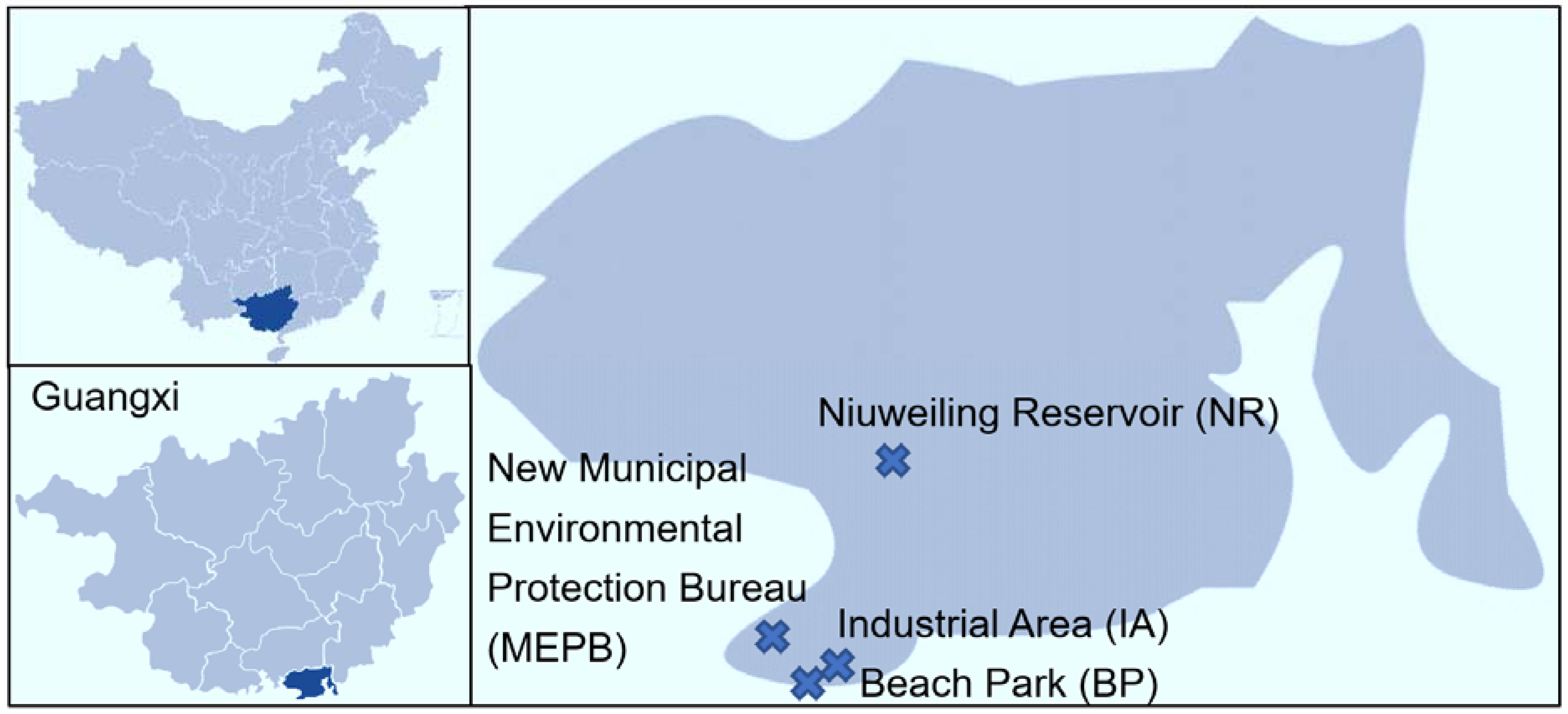
2.1. Study Areas

Beihai is a medium-sized city with huge economic potential located in the south of the Guangxi Zhuang Autonomous Region of China and on the east coast of the most convenient seaport (Beibu Bay) in southwest China (Figure 1). Beihai covers an area of 3337 km2 between 108°50′45″ to 109°47′28″ E, 20°26′ to 21°55′34″ N with a population of 1.68 million, and a Gross Domestic Product (GDP) of 133 billion CNY (BSB, 2019). The urbanization rate of Beihai in 2018 was 58.6% [46]. There are significant differences in the topography of the city: the north is high, with hills; the south is low, with terraces and plains. The difference in topography may be an influencing factor for air pollution transportation. As a port and tourist city, vessel and vehicle exhaust may also play a role in air pollution. Beihai could be a typical example of a less developed city in South China.

2.2. OMI Data

OMI is a new generation of sensors aboard spacecraft on the Aura satellite with a spatial resolution of 13 km × 24 km, jointly developed by the National Aeronautics and Space Administration (NASA) and the Finnish Meteorological Society (FMI), whose major objectives are observations and studies of air quality and the climate change [47]. OMI covers the earth once a day and transits China during the hours of 13:40–13:50 and provides measurements of O3, NO2, SO2, BrO, HCHO as well as aerosols and clouds [48]. Tropospheric NO2 and daily Level-3 SO2 products of the boundary layer vertical column density (VCD) data were derived from OMI and employed in this study. The VCD is the amount of molecules for a specific atmospheric gas from the surface to the height indicated, such as the instrument height [49]. The spatial resolution of the NO2 column concentration is 0.125° × 0.125°, while the daily Level-3 SO2 products are gridded data with a 0.25° × 0.25° spatial resolution on uniform space-time, which is suitable for long-term trend analysis scales [50]. The data format in OMI inversion is HDF (Hierarchy Data Format). It is converted to txt after downloading. Fortran language programming was used to calculate the annual average value of gridding of air pollutants concentrations, and negative, outliers and zero values were removed, and the data within the scope of Beihai were extracted. The average values for 2005–2007, 2008–2010, 2011–2013, 2014–2016, 2017–2019, during the COVID-19 lockdown period (25 January 2020 to 25 February 2020) and during the same period for 2017–2019, and the change trend of the concentration of the pollutants was calculated. Thereafter, the spatial distribution map and the change trend graph of the average concentration of SO2, NO2 and O3 columns were prepared with ArcGIS software.

2.3. Ground Station Measurements and Meteorological Data

The Ministry of Environment and Ecology of China publishes real-time monitoring data of six major pollutants (PM2.5, PM10, O3, SO2, NO2 and CO) in 74 cities since January 2013 [51]. In this study, the hourly PM2.5, PM10, O3, SO2, NO2 and CO concentrations from 2016 to 2020 of four automatic ambient air quality monitoring stations were provided by the Beihai Ecological and Environment Bureau. The measuring stations at Beihai follow the regulations issued by the Ministry of Environment and Ecology [52,53], while quality assurance (QA) and quality control (QC) procedures follow the principles of the National Ambient Air Quality Urban Monitoring Network Management. Daily averages (24 h) and diurnal variation were calculated for the periods during the lockdown (25 January to 25 February in 2020) and before (averaged values of the corresponding period in the previous three years), to analyze the variations in the mean concentration (in μg/m3) between both periods, and their relative change (in %). The names of the monitoring stations, acronyms, geographic locations, the measured species and the periods of data available are summarized in Table 1. Meteorological data including temperature, relative humidity, atmospheric pressure, wind speed and wind direction, were also measured at the four stations, and the hourly data were used in this study.

3. Results and Discussion

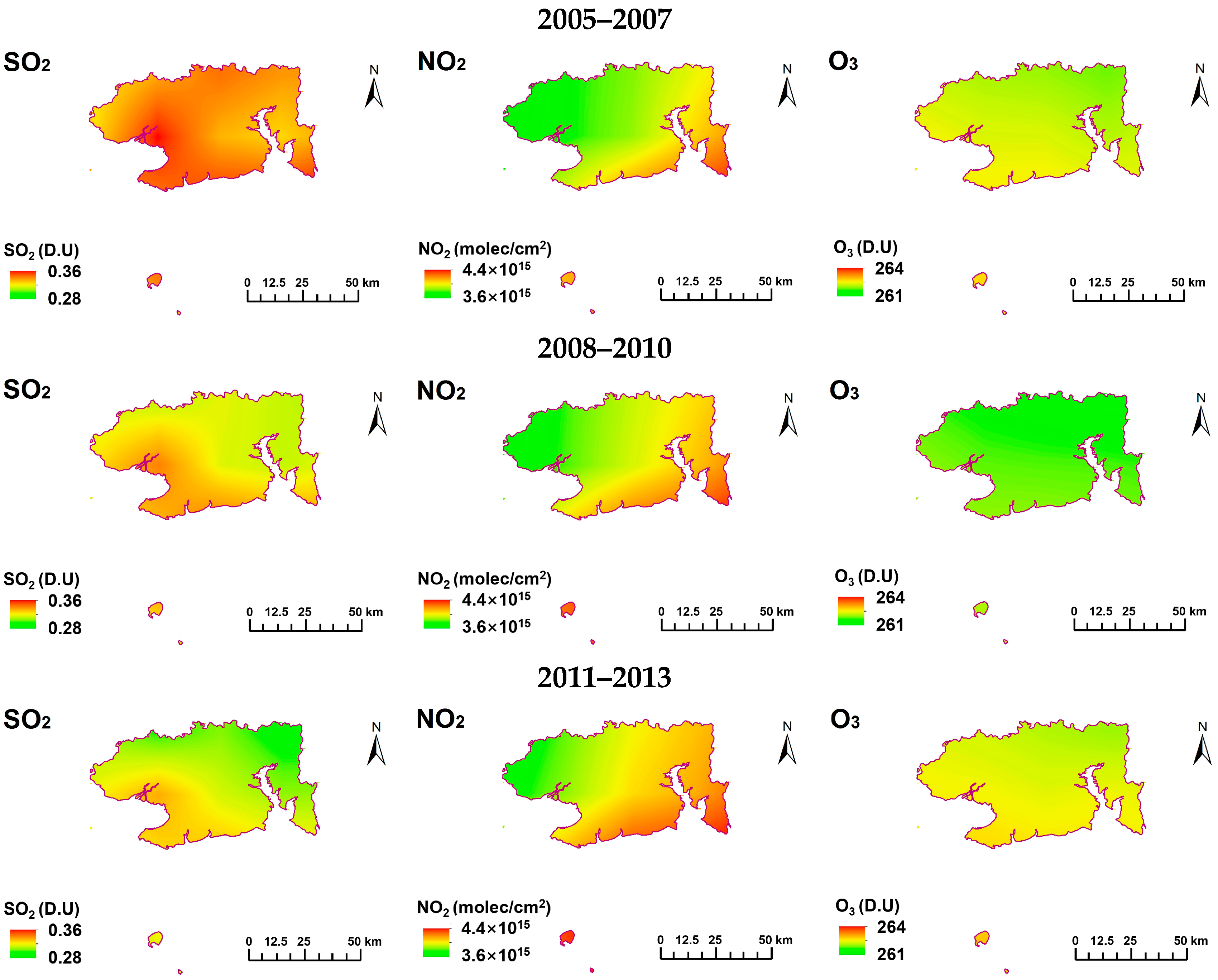
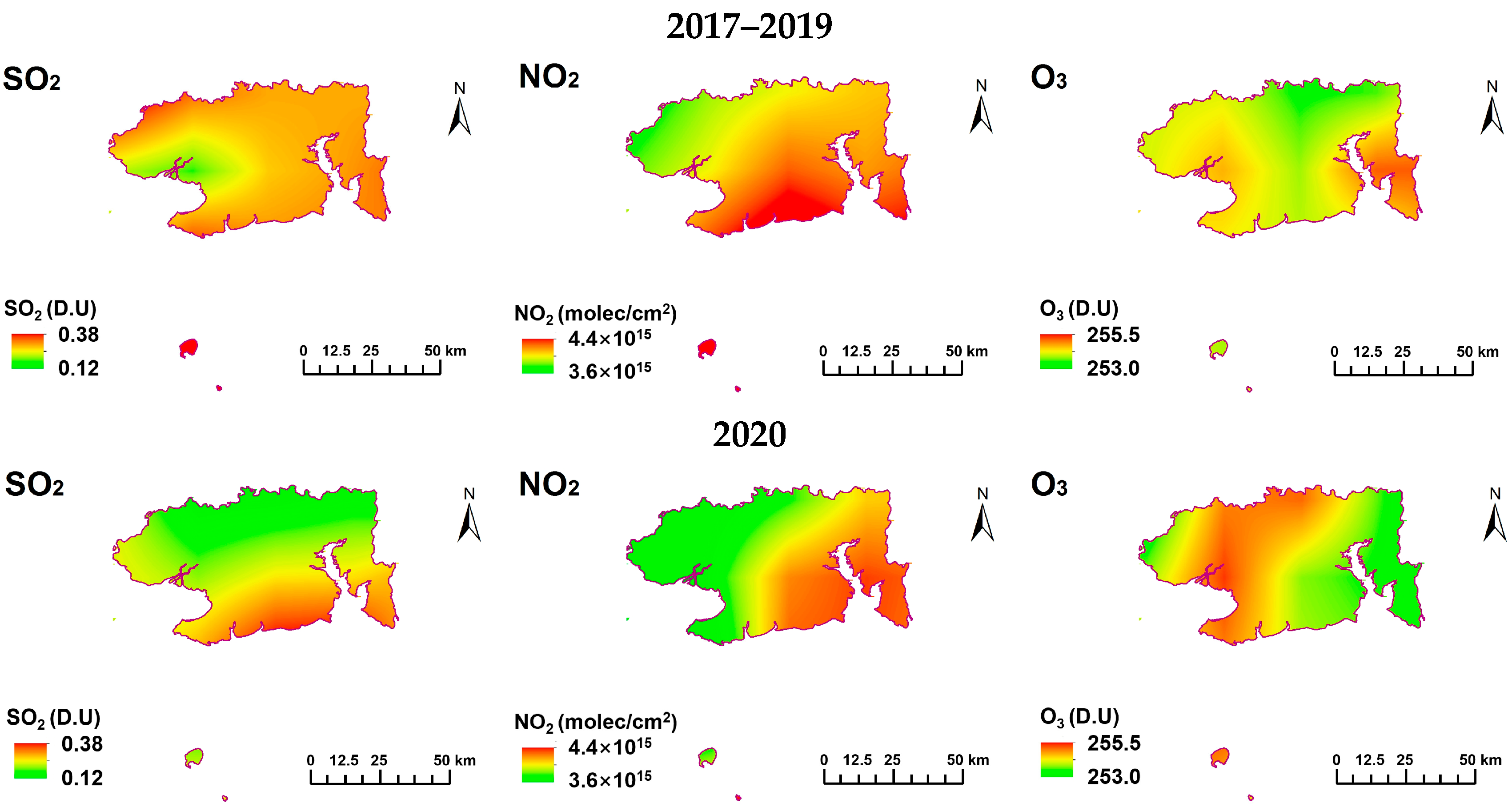
3.1. Spatiotemporal Variation from OMI Observations

Figure 2 depicts the spatial distributions of the averaged VCD SO2, NO2 and O3 on a three-year basis over the past fifteen years. The hotspots of VCD SO2 are mainly centralized in areas near the southwest coast with a high population density and intensive anthropogenic activities (industrialization and urbanization). The SO2 pollution over the area shows a decreasing trend since 2008. Between 2005 and 2007, the average VCD SO2 in Beihai was higher than 0.32 DU (Dobson Units). However, the total areas where the VCD SO2 was below 0.3 DU expanded to more than 2/3 of the total Beihai area by 2019. This decreasing trend is inseparable from a series of policies issued in recent years in China to control the emission of atmospheric pollutants. The major controlling strategy for the SO2 emissions is the phasing out of inefficient coal-fired power generation units and steel plants, the installation of flue gas desulfurization systems in thermal power units, the change of fossil fuel and coal to natural gas, and the implementation of strict emissions standards for densely populated areas and industrial boilers [57,58]. Additionally, particulate matter removal through electrostatic precipitators contributes significantly to the simultaneous reduction in SO2 emissions [59]. On the contrary, the three-year average VCD NO2 increased slightly since 2005 and the NO2 pollution area surrounding the industrial zone near the southeast coast, where the metal and chemical industry and coal-fired power generation are the major industries with high emissions of pollutants, was expanding and the pollution level was rising. The area where the average NO2 column concentration was higher than 4 × 10¹⁵ molecules cm−2 in 2005–2007 accounted for 54.3% of the total Beihai, which expanded to 77.1% by 2017–2019.
With regard to the spatial distributions of O3 during the last fifteen years, apparent high levels of O3 concentrations can be observed in the southwest of Beihai. Tropospheric O3 is generally formed in the atmosphere through photochemical pathways of nitrogen oxides (NOx = NO + NO2) and volatile organic compounds (VOCs) in the presence of sunlight [60]. VOCs emitted from the surrounding chemical bases may also be transmitted to Beihai, influencing the process of photochemical reactions. Due to the complicated and non-linear relationship between O3 and its precursors (NO2 and VOCs) and the complex sources of VOCs in Beihai and surrounding areas including industrial production, vehicle exhaustion, solvent use, and straw burning [61,62], the distribution of severely polluted areas of NO2 and O3 is different, but both demonstrated an increasing trend. During the period of 2008 to 2010, the average VCD O3 decreased slightly (261.74 DU), compared with that of 2005–2007 (262.18 DU), and then increased constantly to 263.58 DU in 2017–2019.
The COVID-19 lockdown measures came into effect in Beihai on 25 January 2020 to flatten the COVID-19 epidemic curve. The social isolation policy issued by the authorities has resulted in reduced anthropogenic activities, including a significant decline in traffic and the suspension of a number of industrial processes. To further investigate the air pollution characteristics of Beihai and to analyze the sources of air pollutants, we assessed the changes in air quality by comparing the air pollutant levels during the COVID-19 lockdown and (25 January 2020 to 25 February 2020) and the averages of those during the same period during the previous three years, as illustrated in Figure 3. During the COVID-19 lockdown, the decrease in the concentration of different air pollutants varies evidently. The averaged VCD NO2 during the lockdown period (3.92 × 10⁻¹⁵ molecules cm−2) decreased by 5.0% when compared with that pre-lockdown (4.12 × 10⁻¹⁵ molecules cm−2). In the case of VCD SO2, the reduction was as high as 22.06% with 0.2222 DU during the lockdown and 0.2851 DU during the same period of the previous three years. In contrast, VCD O3 saw an increase of approximately 4.27% (254.269 DU of the average previous three years and 243.423 DU during the lockdowns).
It could be expected that reduced social activities due to the COVID-19 lockdown temporarily diminished the levels of VCD SO2 and NO2. However, as also shown in Figure 3, areas with high levels of both VCD SO2 and NO2 were situated in the southeast of Beihai, in which the thermal power plant, several essential chemical materials and other industries were located and during the COVID-19 lockdown, these enterprises were completely or largely in operation. This may additionally emphasize the fact that reduced industry and traffic activities due to COVID-19 lockdown temporarily diminished the levels of VCD SO2 and NO2. The levels of VCD O3 saw a significant increment during the COVID-19 lockdown in Beihai. On the one hand, the low levels of nitrogen oxide (NO) around the boundary layer reduce the O3 consumption (titration, NO + O3 = NO2 + O2), thus leading to an increase in O3 concentrations [63,64]; on the other hand, the possible increase of insolation and temperatures from January to February of lockdowns caused an increase in O3 [65], as the first quarter of 2020 in Beihai was the second warmest on record. The stratosphere-troposphere exchange of O3 may, additionally, play a role [66].

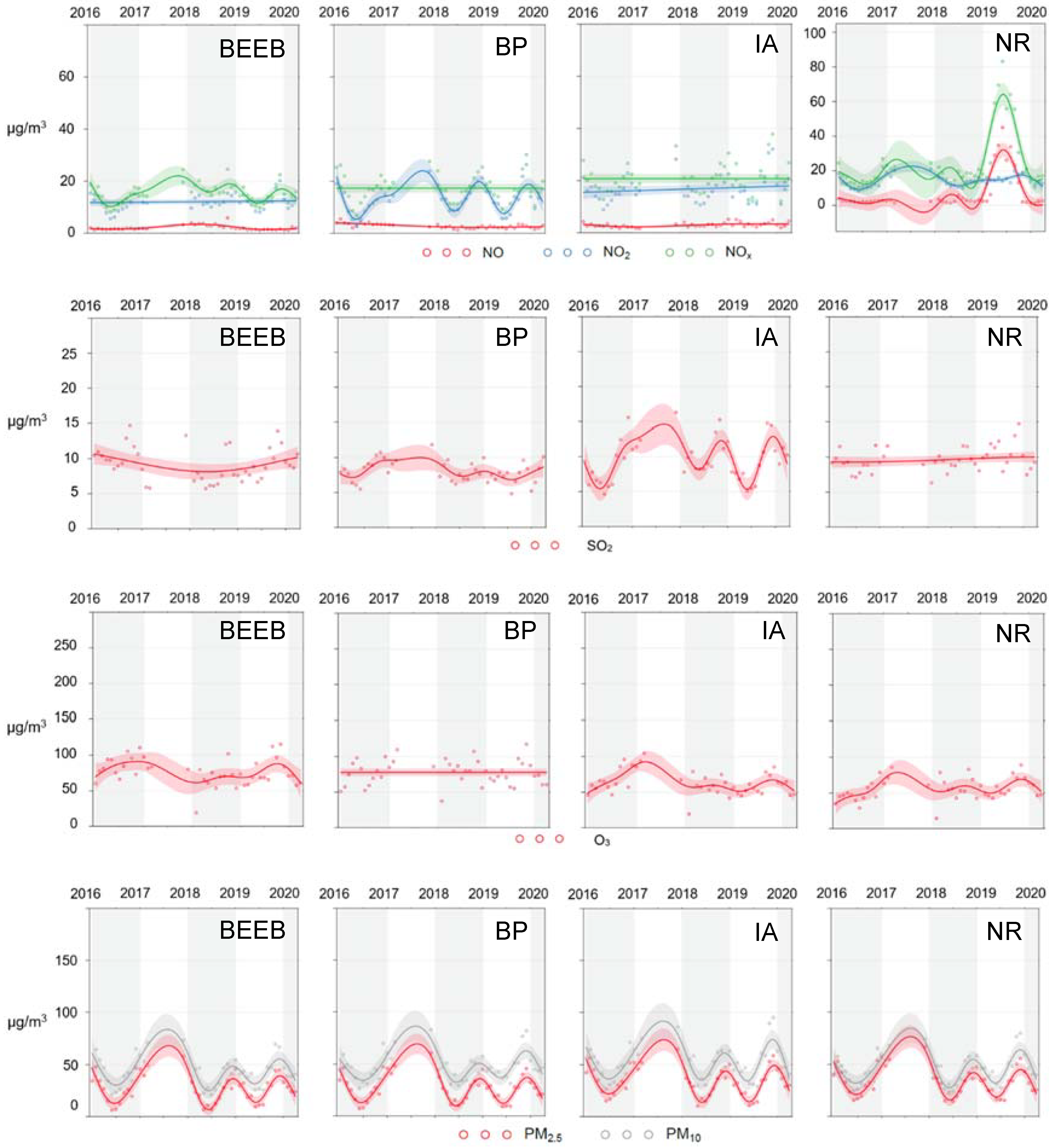
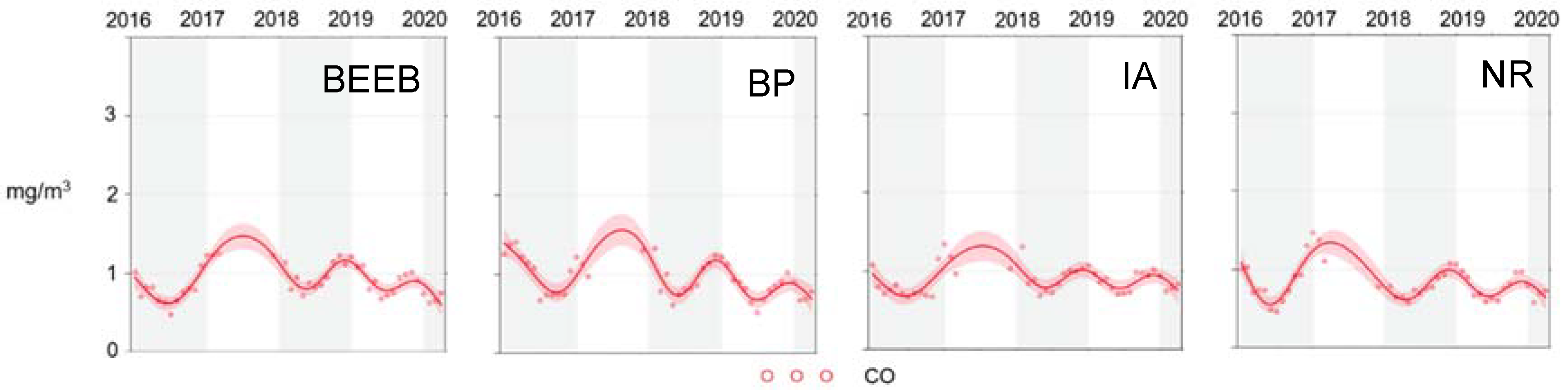
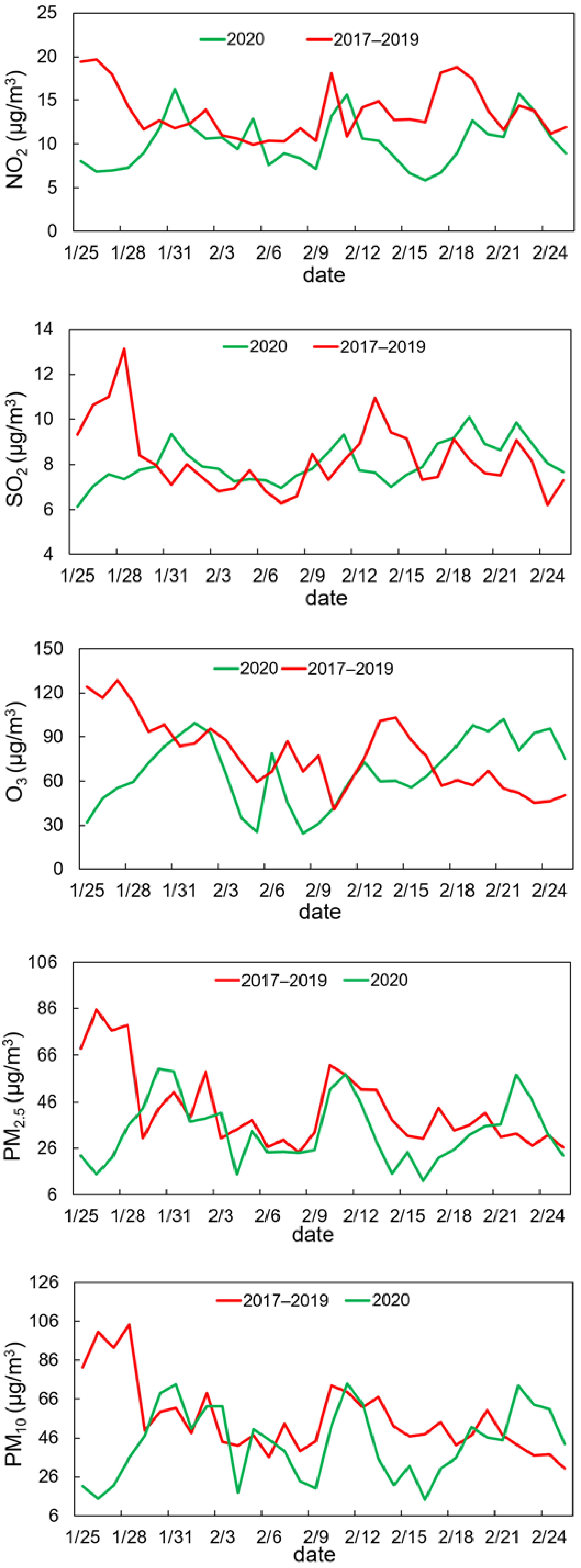
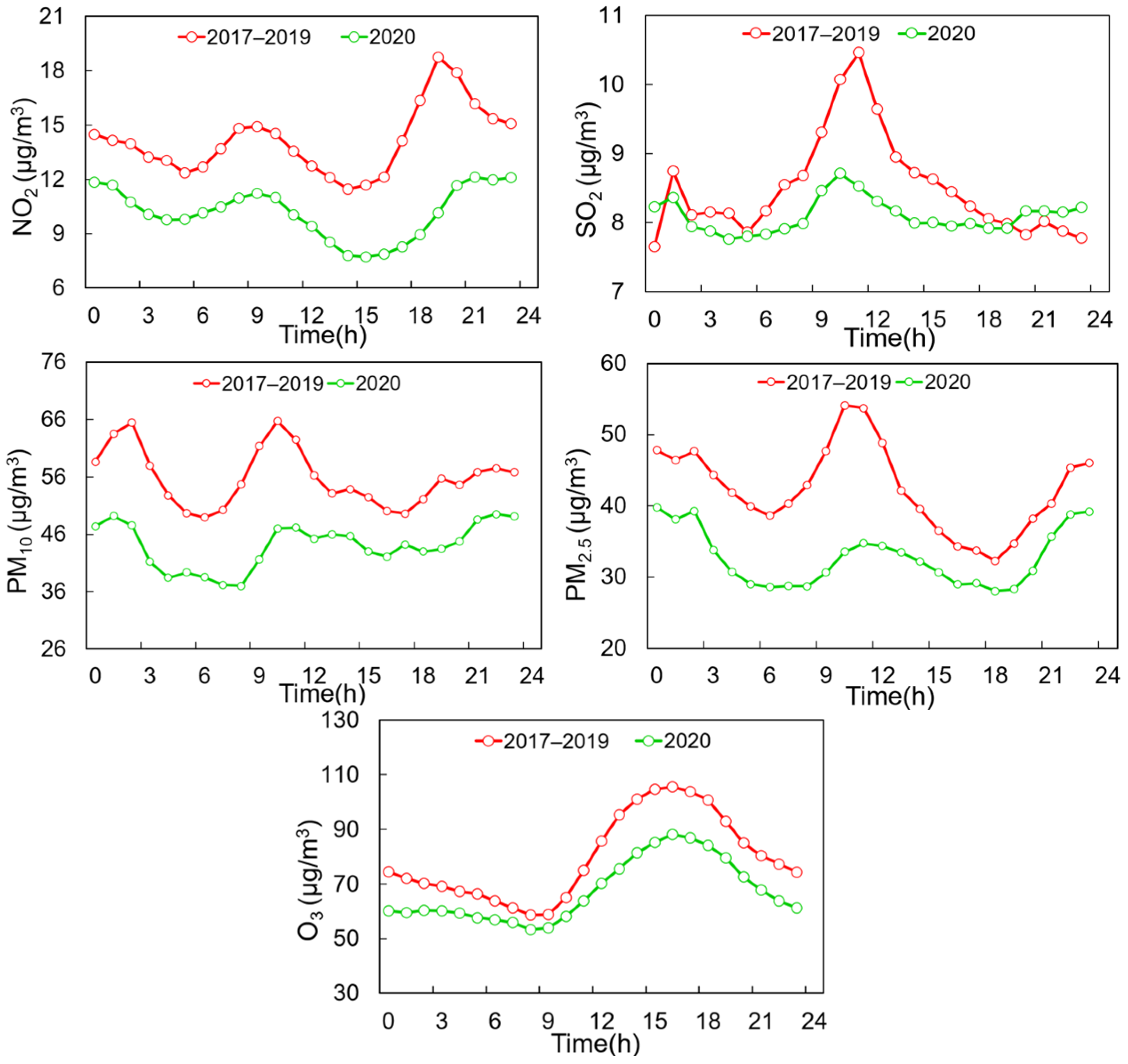
3.2. Long-Term Trends Analysis with Ground Measurements

The concentration data of the measured air pollutants at the four ground observation sites in Beihai were coded to smooth lines to analyze the long-term trends (Figure 4). The smooth line is essentially established on the basis of the Generalized Additive Modelling with “mgcv” package [67]. A plot of monthly concentrations and bands along with the smooth lines in the corresponding color indicate the 95% confidence intervals of the fits. The daily average concentrations of NO over 5 years of all four sites at Beihai varied from 1 μg/m3 (all four stations) and 91.45 μg/m3 (NR), while NO2 concentrations ranged from 1.25 μg/m3 (BP) to 61.08 μg/m3 (BP) and NOx from 3.39 μg/m3 (NR) to 159.45 μg/m3 (NR). Except at the BP station, where a notable fluctuation in nitrogen oxides inter-annual concentrations was recorded, concentrations of nitrogen oxides at the other measurement sites show constant or slightly increasing tendencies. The annual mean NO2 concentration increased from 12.43 μg/m3 in 2016 to 15.45 μg/m3 in 2019. This is consistent with results from OMI. The levels of NO and NOx concentration at the BP station were highly constant, while the NO2 concentrations fluctuated considerably. Ozone concentrations were highest at BEEB (285.74 μg/m3). In contrast to NO2, the concentrations of O3 observed at the BP Station were relatively stable in terms of interannual changes, while at the other three sites, the O3 levels fluctuated significantly and underwent a perceptible increase. The fluctuating trends of PM2.5 and PM10 at the four stations were approximately identical. The daily average concentrations were relatively close at all sites, with PM2.5 varying from 2.08 μg/m3 (BEEB) to 150.73 μg/m3 (IA) and PM10 from 4.42 μg/m3 (IA) to 180.35 μg/m3 (BEEB). The daily mean values of CO concentrations calculated over 5 years never exceeded the Chinese daily Class I Standard of 4 mg/m3 and varied from 0.31 mg/m3 (IA) to 2.05 mg/m3 (BEEB). Decreasing trends of PM2.5, PM10 and CO were observed at all the sites, while the changing trends of SO2 were essentially constant. Only IA witnessed fluctuating inter-annual concentrations of SO2. In summary, the tendencies of all the pollutants measured at ground stations were consistent with the satellite remote sensing observations from the past five years.
Figure 5 shows the comparison between air pollutant concentrations from ground measurements during the COVID-19 lockdown period between 25 January 2020 and 25 February 2020 (LP) and averaged air pollutant concentrations in the same period from 2017–2019 (SP), to identify the contributions of emissions from different sources to air quality in Beihai. The inter-annual variability in air pollution levels could be fully reduced under a three-year (2017–2019) long baseline condition. In general, during the LP, the daily NO2, SO2 and O3 mean concentrations were lower than those during the SP in Beihai; however, the decrease in SO2 concentrations was significantly smaller. The average NO2 and SO2 concentrations decreased during the COVID-19 lockdown by 25.6% (from 13.62 μg/m3 in 2017–2019 to 10.13 μg/m3 in 2020) and 2.7% (from 8.26 μg/m3 in 2017–2019 to 8.03 μg/m3 in 2020), respectively, while O3 also saw a reduction of 13.7% (from 77.84 μg/m3 in 2017–2019 to 67.16 μg/m3 in 2020). The changes in daily NO2 mean concentrations in all the stations in Beihai may be associated with the dramatically reduced road and non-road transportation and the industrial suspension due to recommendations on reducing social contact. Emission data provided by the Beihai Ecological and Environment Bureau (BEEB) have shown that the NOx emissions from the major industrial sources from 25 January to 25 February were 651.0 tons in 2019; this declined to 387.32 tons (40.5% reduction) in 2020. In order to complete the “13th Five-Year Plan” pollution reduction task successfully, the government of the Guangxi Zhuang Autonomous Region has promoted the implementation of ultra-low emission renovation projects for coal-fired power plants vigorously, using integrated technology to remove multiple air pollutants systematically and efficiently [68]. Moreover, most of the projects were completed by 2018. Therefore, power plants in Beihai may not be the main source of air pollutant emissions, but the steel industry could be a considerable contributor. NOx emissions from the petrochemical industry and thermal power plants remained approximately unchanged before and during the COVID-19 outbreak according to the emission data provided by BEEB. Sicard et al. (2020) also observed strong reductions in both NO and NO2 during COVID-19 lockdowns in several European cities, such as Nice, Rome and Valencia [41], which is consistent with our results (NO concentrations decreased by 15.3% and 29.2% in NOx), as shown in Figure S1. A relatively smaller reduction in SO2 concentrations can be explained by the uninterrupted operation of essential industrial activities, such as power plants, steel and petrochemical enterprises; this has also been reflected in the SO2 emission data, as 12.7% less SO2 was emitted during the LP. Although a reduction in automobile emissions was expected, the low sulfur content of automobile gasoline (China V standard, maximum sulfur level of ~10 ppm) implemented since 2017 can weaken the contribution of traffic reduction to decrease in SO2 concentrations. In summary, the reduction in human activity reduced primary air pollutant emissions and led to an improvement in air quality, as also observed by other studies [69,70,71,72]. However, based on the comparison of measurements of air pollutants and emission data of major industries in Beihai, different emission sources may contribute to the reduction in SO2 and NO2. The traffic sector in Beihai may have a limited contribution to the concentration of SO2.
The inconsistency of O3 levels between OMI observations and ground measurements may be due to the difference in observation frequency of the two monitoring techniques and the vertical ozone distribution affected by a number of factors [73]. The local scanning time of the OMI instruments is approximately 13:45 [74] when the O3 concentrations maintain a high level. However, the ground measured O3 concentrations were processed as daily averages. Generally, the O3 formation depends on the VOC-NOx interaction [75]. Previous studies have shown that O3 levels experienced a significant increase during the COVID-19 lockdown in the Yangtze River Delta region [71], Milan [76], Wuhan and a few European cities [41]. In our case, the decrease in daily O3 mean concentrations in Beihai might be associated with reduced ground NO2 concentrations, according to the conclusion demonstrated by Wang et al. (2019) that NOx sensitivity dominated O3 production in the southwest of China [77]. NO serves as the limiting reagent in reactions with RO2 and HO2 and O3 production can be restricted by limiting NOx emissions. During the COVID-19 lockdown, a decrease in ozone precursor emissions, such as VOCs and CO (see Figure S1) reduction, may also have contributed to the ground surface O3 decrease [78,79]. The difference in O3 variations between our observation and other cities could be attributed to the differences in industrial structure and O3 formation mechanisms, e.g., NOx-limited in Beihai [77], while VOCs-sensitive in Wuhan [80].
Figure 5 also provides a daily variation of PM2.5 and PM10 during the LP and SP. An evident decrease in the averaged concentrations of both PM2.5 (−22.2%, from 42.85 μg/m3 in 2017–2019 to 33.3 μg/m3 in 2020) and PM10 (−22.2%, from 56.0 μg/m3 in 2017–2019 to 43.6 μg/m3 in 2020) during the studied period was recorded. PM10 are emitted principally from traffic, industrial processes, construction work and dust entrainment [81,82], whose decrease can presumably reflect the decrease in traffic density and industrial activities (PM2.5), and construction work and dust entrainment (PM2.5–10). The identical reduction rate of PM2.5 and PM10 may suggest a synchronous reduction in both traffic and industrial activities, and construction work and dust entrainment. In additional PM emission data of major industries provided by BEEB, the PM emissions declined by 10.9% (76.85 tons during LP in 2020 and 86.26 tons during the same period in 2019).
Figure 6 further investigated the diurnal variation of the concentration levels of the six air pollutants in Beihai during the LP and SP. The diurnal distribution of NO2 during the LP showed different distribution compared to the SP, and at a much lower level. The NO2 during the SP began to increase at 05:00 and peaked (14.92 μg/m3) at 09:00, which is consistent with the LP, while the second peak during the SP commenced at 16:00 and reached the highest level of the day (18.75 μg/m3) at around 19:00, but a second peak during the LP is not prominent. Generally, increased NO2 concentrations in the atmosphere could be attributed to primary emissions from automobiles and other combustion sources, weak dispersion conditions and the formation of NO2 through the reaction between the primary emitted NO and O3 [18,83]. The increased NO2 concentration during both LP and SP from 06:00 to 09:00 in Beihai could be attributed to elevated traffic emissions and insufficient photochemical consumption of NO2 [18]. The decreasing trend of NO2 concentrations between 09:00 and 15:00 can be caused by the increased photochemical reaction of O3 production from NO2 and VOCs accompanied by high temperatures, the increase in solar radiation, and the boundary layer height [84,85]. High dispersion and high dilution conditions resulting from the high temperature during the mid-day time may consequently enhance the thermal turbulence and thus lead to a decrease in NO2 concentrations. After intensive photochemical consumption of NO2, enhanced anthropogenic activities, particularly automobile emissions may be responsible for the rise and peak of the NO2 concentrations. During evening and nighttime until early morning, the boundary layer descends and resists the mixing of NO2 emissions with the upper layer, thereby resulting in high levels of NO2 [86]. The much lower levels of NO2 concentrations during the LP and the absence of an evening peak may highlight the reduced impact of emissions from the traffic sector on the NO2 concentrations during the COVID-19 lockdown in Beihai.
It can be noticed from Figure 6 that the diurnal variation of O3 during both the LP and the SP is a typical signature of high concentrations during the daytime and low concentrations during the late night and early morning. The lowest O3 concentration during both the LP and SP appears around the morning hours (07:00–09:00), while they peaked at about 16:00, which is essentially opposite to the distribution of the ozone precursor, NO2. A similar diurnal variation pattern of O3 has been reported in numerous studies worldwide [87,88,89,90]. Solar radiation intensity increases in the daytime and favors the conditions to power the photochemical conversion to O3. The low level of O3 concentration during late night and morning is related to the consumption of O3 by deposition and or reaction with NO and NO2 and the absence of the photochemical reactions [91]. The diurnal patterns of O3 for the LP and SP show a similar pattern; however, the levels during lockdown were much lower, which may be attributed to the low levels of ozone precursors (NOx and VOCs emissions) resulting from limited traffic and various industrial activities.
The SO2 concentration in Beihai during the LP and SP shows a single mode diurnal variation, and an evident lower level of SO2 during the LP is observed, e.g., the peak SO2 concentration during the SP was 16.7% higher than that during the SP. However, the SO2 concentrations between 20:00 and 00:00 during the LP were slightly higher than those during the SP. This may not be a result of an increase in the SO2 emissions, because the traffic and industrial activities saw an evident fall during the COVID-19 lockdown. Meteorological conditions, such as the boundary layer height [6], might be responsible for the high level of SO2 concentrations during the nighttime.
In the case of PM2.5 and PM10, the diurnal variations of PM2.5 and PM10 during the LP and SP were highly identical, but the concentration levels of both PM2.5 and PM10 during the LP were evidently lower. The PM2.5 concentrations during the daytime were perceptibly lower than the nighttime during the LP, which is the opposite of that during the SP. This may be because of the reduction in primary PM2.5 emissions due to reduced vehicle and industrial activities and the accumulation effect during the nighttime [92]. Additionally, the reduction rate of coarse particles (PM2.5–10) is approximately the same as PM2.5, which may suggest a proportional reduction in coarse particle emissions, such as construction [93].

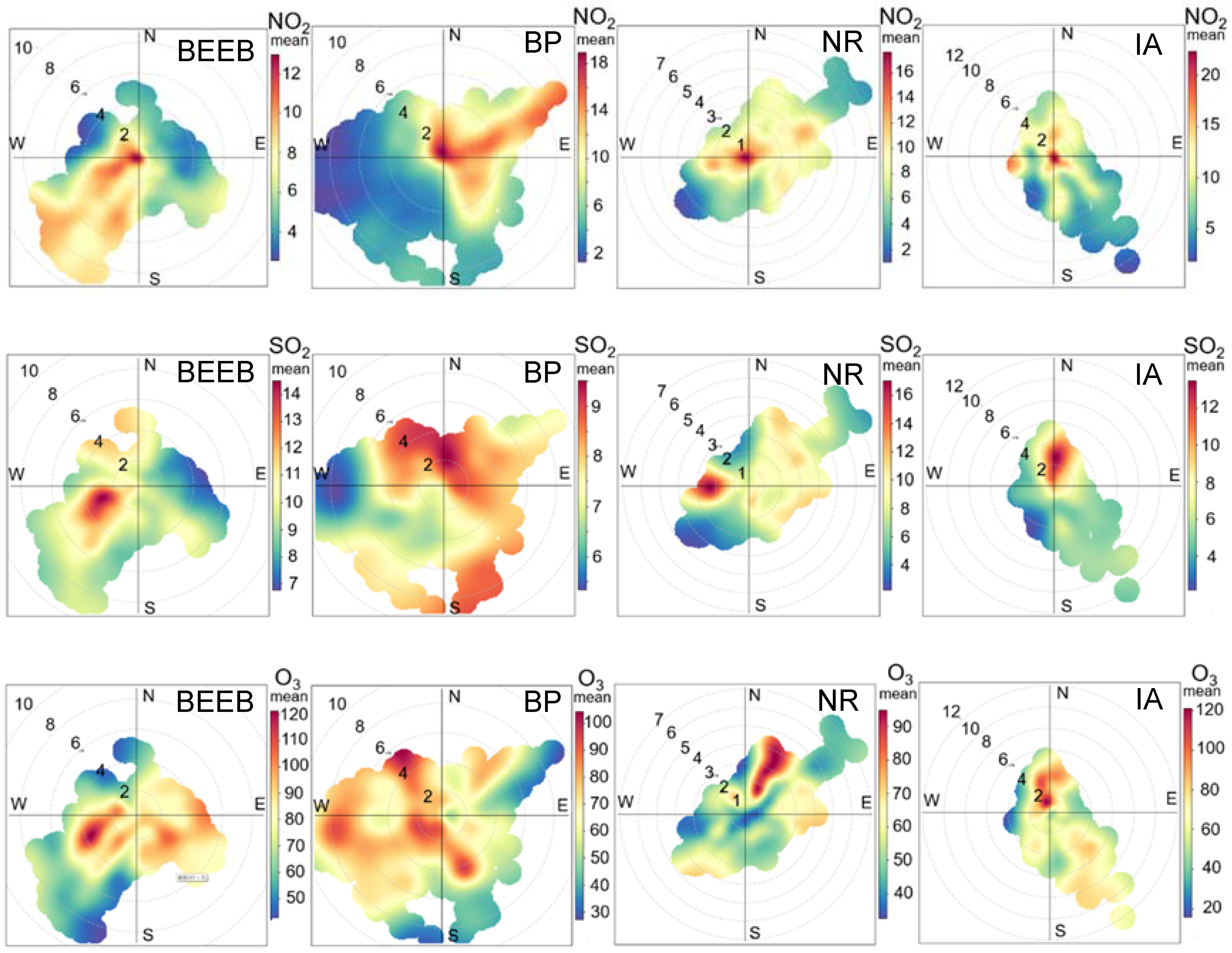
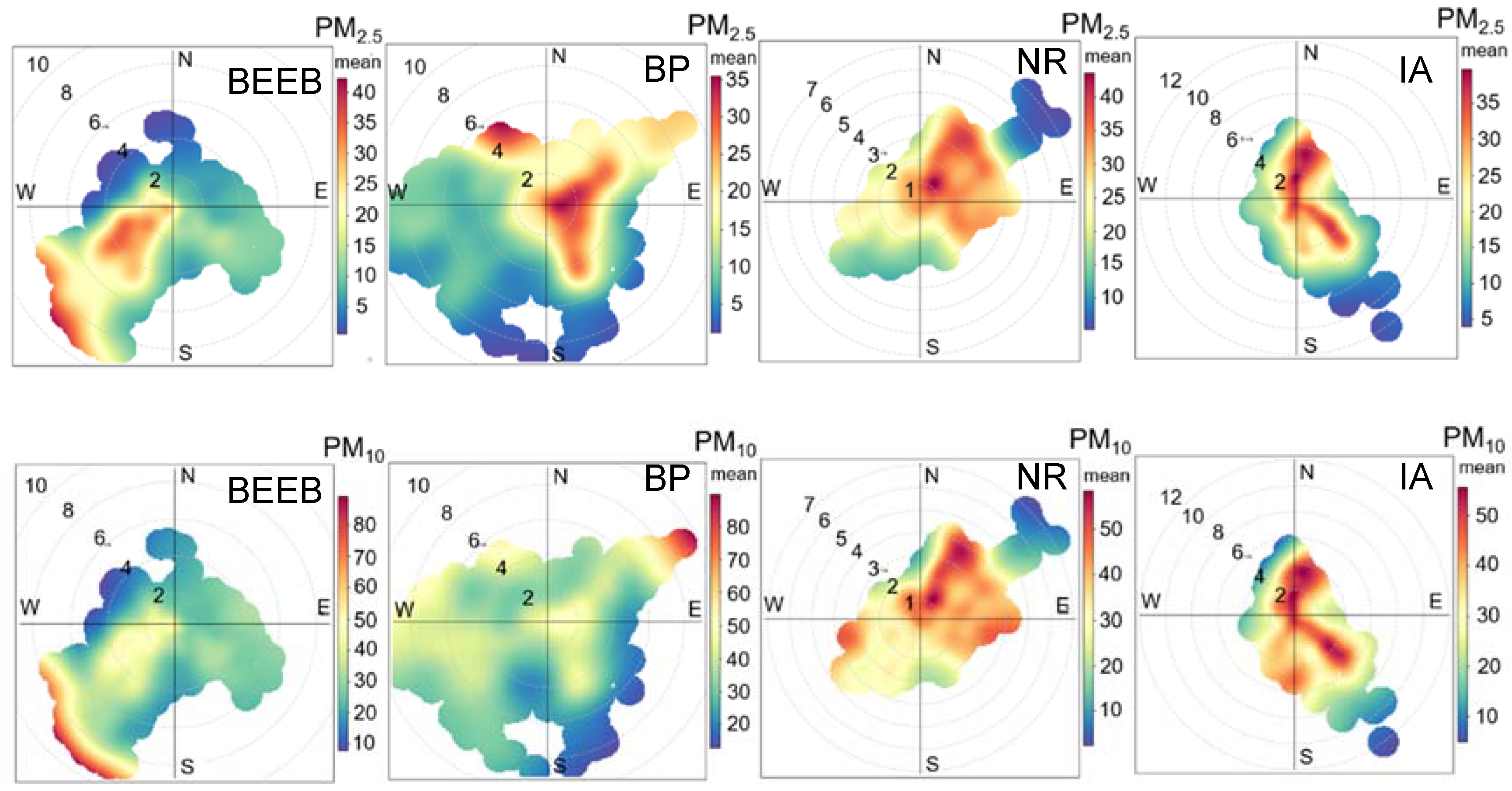
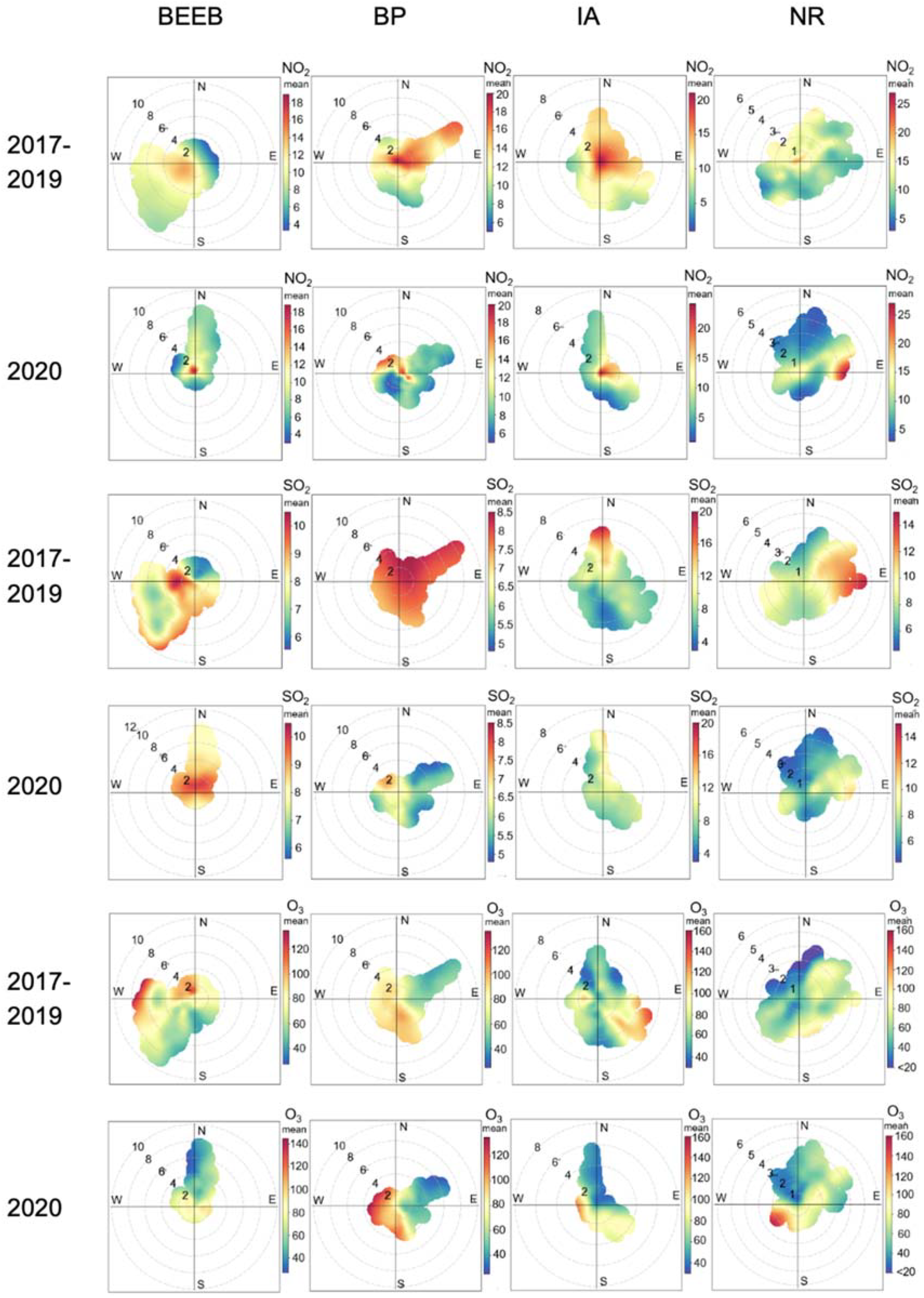
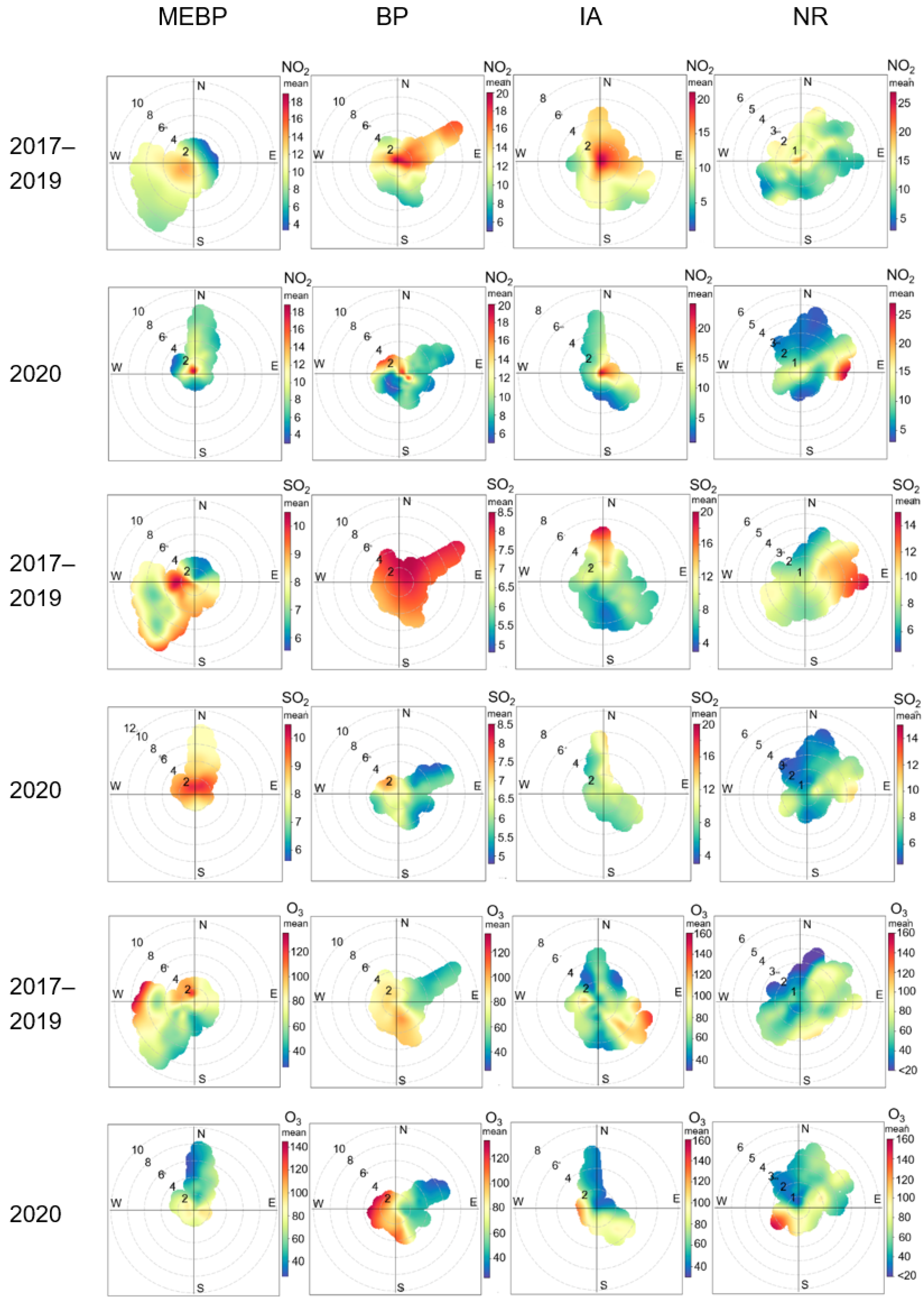
3.3. Source Apportionment with Polar Plot Analysis

The potential sources of atmospheric pollutants at four ground observation sites are generally investigated preliminarily by bivariate polar plots analysis, which is a valuable statistical tool for mapping the pollutant concentrations as a continuous surface by wind speed and direction [55,94]. These polar plots provide a reference for the directional dependence of different sources and the variation of air pollutant concentrations with respect to wind speed and direction [67,95]. Polar plots were computed for four sites with hourly measured data from 1 January 2016 to 25 February 2020, as illustrated in Figure 7.
Polar plots at the BEEB station show the highest concentrations of both gaseous and particulate pollutants when the wind comes from the northwest. The prevailing air pollutant emission sources from the northwest are a fishing port zone integrating fishing boats, aquatic product processing, and fishery tourism, a cargo terminal, a major motor road, residual areas and an industrial park including rubber and plastic production plants, as well as an electronic company. Polar plots at the BP station showed very different variation characterization compared to those at the BEEB. SO2 in the BP station exhibited high concentrations from all wind directions except for west and southwest but increased towards the northeast and northwest. A major motor road with a bus station and the Beihai Yintan tourist area with a sophisticated transportation system lies near the north of this measuring site, which may lead to the transport of SO2 emissions toward the observatory site.
Evident high SO2 concentrations in the IA station (12–13 μg/m3) were also observed with increases from the north under a range of wind speeds (0 to 8 m/s). The location of IA is near numerous emission sources including the power plant and oil refinery facilities on the north side. Similarly, elevated SO2 concentrations in the NR site were observed from the west and south due to the stack emissions from the industrial park (~4.7 km) in the near west, and the industrial area and main motor roads on the south side. Ozone precursors, such as NOx and VOCs produced from an industrial area in the north and the highway extending northeast from the site may be the reason for the higher O3 concentration when the station is exposed to the northeast wind.
Bivariate polar plots for PM2.5 and PM10 are largely identical at the IA and NR stations, demonstrating similar prevailing sources and that the majority of PM10 is mainly made up of PM2.5. PM2.5/PM10 was 0.69 at the IA station and 0.80 at the NR station, indicating the dominant contribution of fine particles to PM episodes. The expressway in the northeast might have caused higher PM2.5 and PM10 concentrations near the NR station during the northeast wind. Vehicle emissions on the main road in the northeast and residential areas in the southeast may lead to higher PM2.5 and PM10 concentrations when the IA station is exposed to the northeast and southeast winds. The PM10 concentration was highest under high wind speed (>8 m/s) at both the BEEB and BP stations, which are located in urban areas. This may indicate that high PM10 concentrations at the BEEB and BP were dominantly transported from northwest and southwest, and northeast, respectively.
Uria-Tellaetxe and Carslaw [96] pointed out that when non-buoyant ground-level sources, such as road traffic emissions and domestic heating are the major emissions sources, high NO2 concentrations are likely to occur under stable atmospheric conditions. The highest NO2 concentrations occur under very low wind speed conditions and show little directional dependence at all four stations, which indicates non-buoyant ground-level sources are the main contributors to NO2 emissions rather than long transportation, such as local traffic. Additionally, the evident distinction between the two main peak concentration levels of NO2 during the LP and SP may also emphasize the highlighted impact of traffic on the NO2 levels. With regard to O3, the polar plots of O3 show an approximately opposite pattern to that of NOx (Figure S2 and NO2 at all sites, due to the titration by NOx [97]. The O3 levels are lower in stable atmospheric conditions (at very low wind speed) and show the highest concentration when the wind is blowing from a certain direction, which is an opposite trend to that of NOx and NO2.
To further analyze the sources of atmospheric pollutants, we generated polar plots for the LP and SP, as shown in Figure 8. Evident discrepancies in the concentration distribution depending on wind speed and wind direction during the LP and SP are observed. The highest NO2 concentrations occur under very low wind speed at all four sites during the lockdown, while higher NO2 levels occurred from certain wind directions during the SP, such as the higher concentrations when the wind comes from the northwest at the BEEB and the southeast at the BP, which is consistent with the long-term polar plot characteristics described above. This may highlight a more significant impact of local sources (traffic particularly) on NO2 concentrations than transportation during the LP. SO2 exhibited high concentrations from the same wind direction during the LP and SP. The closure of non-essential businesses, such as tourist sites, motorized transport, residential emissions and bus traffic might lead to the high SO2 levels at the BP, and stack emissions from industrial plants and main traffic roads might be responsible for high SO2 levels at the IA and NR. In short, high concentrations of SO2 were observed at lower wind speed during the LP, suggesting the contribution of local emission sources to SO2 during the LP. Similarly, high concentrations of PM2.5 and PM10 were observed at lower wind speeds during the LP, and under relatively high wind speeds during the SP. Low wind speeds are beneficial for the PM2.5 accumulation from traffic around monitoring sites [98]. PM10 concentrations were low when high winds occur, which was probably due to resuspension [98]. Moreover, the wind direction leading to the higher concentration was also different between the LP and SP, e.g., the highest PM10 concentrations were observed when the wind was blowing from the northeast under a speed range of 8 to 10 m/s during the SP at BP, while PM10 concentrations were highest under wind speeds of 2–4 m/s from the northwest during the LP, all of which indicate that the sources of particulate matter were different during the LP compared with those during the SP and there were probably more local emissions. Bivariate polar plots for O3 also showed the different sources of O3 between the LP and SP. At the IA station, high O3 concentrations were observed when the wind came from the west during the SP, while high O3 concentrations were observed when the wind came from the west during the LP; the O3 peak values during the LP were much higher. The west of the IA station is a major traffic road in Beihai, which may indicate that the decrease in NOx caused by traffic limitation might be the cause of the decrease in O3 concentrations.

4. Conclusions

Mass suspension of human activities for a long period is extremely rare, the COVID-19 lockdown serves as a natural experiment to investigate the impact of anthropogenic activities on air quality. This study initiated a novel synthesis of multiple-year satellite observations; national-station ground measurements of SO2, NO2 and O3, and meteorological conditions to address the impact of the COVID-19 lockdown in Beihai, a specific city in a less developed area in southwest China, to reveal the potential implications for the control strategies of air pollution. The changing trends in pollution levels (SO2, NO2 and O3) and spatial distribution on a 15-year basis over Beihai were characterized, while satellite retrieved and ground measurements of major air pollutants during the lockdown period and those during the same period of previous years were compared to identify the impact of the COVID-19 lockdown in Beihai; a series of statistical tools were applied to analyze the potential sources and to obtain a comprehensive understanding of air pollution status, to reveal potential implications for more effective control strategies of air pollution.
Results show that satellite observed SO2 pollution saw a decrease since 2005, while NO2 and O3 showed an increasing trend during the last 15 years, which is consistent with the trend of ground measurements. A comparison between the NO2 and SO2 levels during the COVID-19 lockdown period and those during the same period over 2017–2019 shows that VCD NO2 decreased by 5.26%, while VCD SO2 saw a reduction of 22.06%. With regard to the ground measurements of air pollutants, the daily mean concentrations of NO2 SO2, PM2.5 and PM10 during the LP were 25.6%, 2.7%, 22.2% and 22.2%, lower, respectively, than those during the SP. Averaged VCD O3 during the LP increased by 4.26%; however, ground measured daily O3 mean concentrations saw a decrease of 13.7%. The discrepancies in O3 concentrations between satellite observations. Ground measured SO2 concentrations during the LP were only 2.7% lower than those during the SP, which may be attributed to uninterrupted essential industrial activities, such as power plants. The traffic sector in Beihai may have a limited contribution to the concentration of SO2. The highest NO2 concentrations occurred under very low wind speed and showed little directional dependence at all four stations, indicating non-buoyant ground-level sources could be the main contributor to NO2 concentration. Additionally, the much lower levels of NO2 during the LP and the absence of an evening peak may highlight the significant impact of the traffic sector on the NO2 concentration. The decrease in the daily O3 mean concentration during the LP might be associated with the reduction in NO2 concentrations, as NOx sensitivity is found to be dominated in O3 formation in the northwest part of China, which is different from other cities, e.g., Shanghai. Hence, the reduction of O3 in Beihai could be coordinated with NOx reduction in terms of traffic controls. This study assessed the impact of the COVID-19 lockdown on air quality in Beihai and the implications of this study could be beneficial to the formulation of atmospheric protection policies.

Supplementary Materials

The following supporting information can be downloaded at: https://0-www-mdpi-com.brum.beds.ac.uk/article/10.3390/atmos13050842/s1, Figure S1. Daily CO and NOx mean concentrations of all four stations in Beihai between 25 January and 25 February averaged over previous three years (2017–2019, red line) and in 2020 (the COVID-19 lockdown), Figure S2. Diurnal variation of CO and NOx concentrations Beihai in Beihai between 25 January and 25 February averaged over previous three years (2017–2019, red line) and in 2020 (the COVID-19 lockdown), Figure S3. Bivariate polar plots of CO and NOx for four observation sites, Figure S4. Bivariate polar plots of CO and NOx for four observation sites from 25 January to 25 February in 2017–2019 and in 2020.

Author Contributions

Conceptualization: X.J. and H.X.; Methodology: X.J., H.X. and M.G.; Software: J.L., J.W. and L.F.; Data Curation and visualization: X.H., Q.D. and Y.Y.; Validation: X.H., Q.D., H.R. and G.Q.; Writing—original draft preparation: H.X. and X.J.; Writing—review and editing: L.F., J.C. and H.R.; Funding acquisition: J.C.; Resources: G.Q. and Y.Y.; Supervision: J.C. All authors have read and agreed to the published version of the manuscript.

Funding

This work was funded by Beihai Ecological and Environmental Bureau (G-BZGC004-20180201), China Institute of Urban Governance, Shanghai Jiao Tong University (Key Special Project of China, No. SJTU-2019UGBD-01), Tianjin Municipal Transportation Commission (Project No. 2022-23) and Tianjin Research Institute for Water Transport Engineering, Ministry of Transport (Project No. TKS20220501).

Institutional Review Board Statement

Not applicable.

Informed Consent Statement

Not applicable.

Data Availability Statement

All data generated or analyzed during this study are included in this published article and its supplementary information files.

Acknowledgments

The present work was funded by Beihai Ecological and Environmental Bureau (G-BZGC004-20180201), China Institute of Urban Governance, Shanghai Jiao Tong University (Key Special Project of China, No. SJTU-2019UGBD-01), Tianjin Municipal Transportation Commission (Project No. 2022-23) and Tianjin Research Institute for Water Transport Engineering, Ministry of Transport (Project No. TKS20220501). The authors gratefully acknowledge the funders. The publication’s contents do not necessarily represent the views of the sponsors.

Conflicts of Interest

The authors declare no conflict of interest.

References

  1. Kjellstrom, T.; Friel, S.; Dixon, J.; Corvalan, C.; Rehfuess, E.; Campbell-Lendrum, D.; Gore, F.; Bartram, J. Urban environmental health hazards and health equity. J. Urban Health Bull. N. Y. Acad. Med. 2007, 84, 86–97. [Google Scholar] [CrossRef] [PubMed] [Green Version]
  2. Moore, M.; Gould, P.; Keary, B.S. Global urbanization and impact on health. Int. J. Hyg. Environ. Health 2003, 206, 269–278. [Google Scholar] [CrossRef] [PubMed]
  3. Xiao, K.; Wang, Y.; Wu, G.; Fu, B.; Zhu, Y. Spatiotemporal Characteristics of Air Pollutants (PM10, PM2.5, SO2, NO2, O3, and CO) in the Inland Basin City of Chengdu, Southwest China. Atmosphere 2018, 9, 74. [Google Scholar] [CrossRef] [Green Version]
  4. Guo, H.; Gu, X.; Ma, G.; Shi, S.; Wang, W.; Zuo, X.; Zhang, X. Spatial and temporal variations of air quality and six air pollutants in China during 2015–2017. Sci. Rep. 2019, 9, 15201. [Google Scholar] [CrossRef] [Green Version]
  5. Chudnovsky, A.; Tang, C.; Lyapustin, A.; Wang, Y.; Schwartz, J.; Koutrakis, P. A critical assessment of high-resolution aerosol optical depth retrievals for fine particulate matter predictions. Atmos. Chem. Phys. 2013, 13, 10907–10917. [Google Scholar] [CrossRef] [Green Version]
  6. Zheng, C.; Zhao, C.; Li, Y.; Wu, X.; Zhang, K.; Gao, J.; Qiao, Q.; Ren, Y.; Zhang, X.; Chai, F. Spatial and temporal distribution of NO2 and SO2 in Inner Mongolia urban agglomeration obtained from satellite remote sensing and ground observations. Atmos. Environ. 2018, 188, 50–59. [Google Scholar] [CrossRef] [Green Version]
  7. Guo, H.; Cheng, T.; Gu, X.; Chen, H.; Wang, Y.; Zheng, F.; Xiang, K. Comparison of Four Ground-Level PM2.5 Estimation Models Using PARASOL Aerosol Optical Depth Data from China. Int. J. Environ. Res. Public. Health 2016, 13, 180. [Google Scholar] [CrossRef] [Green Version]
  8. Zhang, X.; Sun, J.; Wang, Y.; Li, W.; Zhang, Q.; Wang, W.; Quan, J.; Cao, G.; Wang, J.; Yang, Y.; et al. Factors contributing to haze and fog in China. Chin. Sci. Bull. 2013, 58, 1178–1187. [Google Scholar]
  9. Zhao, X.J.; Zhao, P.S.; Xu, J.; Meng, W.; Pu, W.W.; Dong, F.; He, D.; Shi, Q.F. Analysis of a winter regional haze event and its formation mechanism in the North China Plain. Atmos. Chem. Phys. 2013, 13, 5685–5696. [Google Scholar] [CrossRef] [Green Version]
  10. Chang, Y. China needs a tighter PM2.5 limit and a change in priorities. Environ. Sci. Technol. 2012, 46, 7069–7070. [Google Scholar] [CrossRef] [Green Version]
  11. Hystad, P.; Demers, P.A.; Johnson, K.C.; Carpiano, R.M.; Brauer, M. Long-term Residential Exposure to Air Pollution and Lung Cancer Risk. Epidemiology 2013, 24, 762–772. [Google Scholar] [CrossRef] [PubMed]
  12. Kermani, M.; Dowlati, M.; Jonidi, J.A.; Rezaei Kalantari, R. Health Impact Caused by Exposure to Particulate Matter in the Air of Tehran in the Past Decade. Tehran Univ. Med. J. TUMS Publ. 2017, 74, 885–892. Available online: http://tumj.tums.ac.ir/article-1-7886-en.html (accessed on 8 August 2020).
  13. Kurt, O.K.; Zhang, J.; Pinkerton, K.E. Pulmonary health effects of air pollution. Curr. Opin. Pulm. Med. 2016, 22, 138–143. [Google Scholar] [CrossRef] [PubMed]
  14. Stanek, L.W.; Brown, J.S.; Stanek, J.; Gift, J.; Costa, D.L. Air pollution toxicology—A brief review of the role of the science in shaping the current understanding of air pollution health risks. Toxicol. Sci. Off. J. Soc. Toxicol. 2011, 120, 8–27. [Google Scholar] [CrossRef]
  15. Alvarellos, A.; Chao, A.L.; Rabuñal, J.R.; García-Vidaurrázaga, M.D.; Pazos, A. Development of an Automatic Low-Cost Air Quality Control System: A Radon Application. Appl. Sci. 2021, 11, 2169. [Google Scholar] [CrossRef]
  16. ul-Haq, Z.; Tariq, S.; Ali, M. Tropospheric NO2 Trends over South Asia during the Last Decade (2004–2014) Using OMI Data. Adv. Meteorol. 2015, 2015, 959284. [Google Scholar] [CrossRef] [Green Version]
  17. Wang, Y.G.; Ying, Q.; Hu, J.; Zhang, H. Spatial and temporal variations of six criteria air pollutants in 31 provincial capital cities in China during 2013–2014. Environ. Int. 2014, 73, 413–422. [Google Scholar] [CrossRef]
  18. Song, C.; Wu, L.; Xie, Y.; He, J.; Chen, X.; Wang, T.; Lin, Y.; Jin, T.; Wang, A.; Liu, Y.; et al. Air pollution in China: Status and spatiotemporal variations. Environ. Pollut. 2017, 227, 334–347. [Google Scholar] [CrossRef]
  19. Wallace, J.; Corr, D.; Kanaroglou, P. Topographic and spatial impacts of temperature inversions on air quality using mobile air pollution surveys. Sci. Total Environ. 2010, 408, 5086–5096. [Google Scholar] [CrossRef]
  20. Zhang, Z.; Zhang, X.; Gong, D.; Quan, W.; Zhao, X.; Ma, Z.; Kim, S.J. Evolution of surface O3 and PM2.5 concentrations and their relationships with meteorological conditions over the last decade in Beijing. Atmos. Environ. 2015, 108, 67–75. [Google Scholar] [CrossRef]
  21. Cai, L.; Zhuang, M.; Ren, Y. Spatiotemporal characteristics of NO2, PM2.5 and O3 in a coastal region of southeastern China and their removal by green spaces. Int. J. Environ. Health Res. 2020, 32, 1–17. [Google Scholar] [CrossRef] [PubMed]
  22. Jiang, L.; Bai, L. Spatio-temporal characteristics of urban air pollutions and their causal relationships: Evidence from Beijing and its neighboring cities. Sci. Rep. 2018, 8, 1279. [Google Scholar] [CrossRef] [Green Version]
  23. Liu, F.; Beirle, S.; Zhang, Q.; van der A, R.J.; Zheng, B.; Tong, D.; He, K. NOx emission trends over Chinese cities estimated from OMI observations during 2005 to 2015. Atmos. Chem. Phys. 2017, 17, 9261–9275. [Google Scholar] [CrossRef] [PubMed] [Green Version]
  24. Russell, A.R.; Valin, L.C.; Cohen, R.C. Trends in OMI NO2 observations over the United States: Effects of emission control technology and the economic recession. Atmos. Chem. Phys. 2012, 12, 12197–12209. [Google Scholar] [CrossRef] [Green Version]
  25. Li, C.; Zhang, Q.; Krotkov, N.A.; Streets, D.G.; He, K.; Tsay, S.C.; Gleason, J.F. Recent large reduction in sulfur dioxide emissions from Chinese power plants observed by the Ozone Monitoring Instrument. Geophys. Res. Lett. 2010, 37, L08807. [Google Scholar] [CrossRef] [Green Version]
  26. Li, C.; McLinden, C.; Fioletov, V.; Krotkov, N.; Carn, S.; Joiner, J.; Streets, D.; He, H.; Ren, X.; Li, Z.; et al. India Is Overtaking China as the World’s Largest Emitter of Anthropogenic Sulfur Dioxide. Sci. Rep. 2017, 7, 14304. [Google Scholar] [CrossRef] [Green Version]
  27. Damiani, A.; De Simone, S.; Rafanelli, C.; Cordero, R.R.; Laurenza, M. Three years of ground-based total ozone measurements in the Arctic: Comparison with OMI, GOME and SCIAMACHY satellite data. Remote Sens. Environ. 2012, 127, 162–180. [Google Scholar] [CrossRef]
  28. Li, R.; Cui, L.; Li, J.; Zhao, A.; Fu, H.; Wu, Y.; Zhang, L.; Kong, L.; Chen, J. Spatial and temporal variation of particulate matter and gaseous pollutants in China during 2014–2016. Atmos. Environ. 2017, 161, 235–246. [Google Scholar] [CrossRef]
  29. Wang, J.; Hu, Z.; Chen, Y.; Chen, Z.; Xu, S. Contamination characteristics and possible sources of PM10 and PM2.5 in different functional areas of Shanghai, China. Atmos. Environ. 2013, 68, 221–229. [Google Scholar] [CrossRef]
  30. Wang, M.; Cao, C.; Li, G.; Singh, R.P. Analysis of a severe prolonged regional haze episode in the Yangtze River Delta, China. Atmos. Environ. 2015, 102, 112–121. [Google Scholar] [CrossRef]
  31. Zheng, J.; Zhang, L.; Che, W.; Zheng, Z.; Yin, S. A highly resolved temporal and spatial air pollutant emission inventory for the Pearl River Delta region, China and its uncertainty assessment. Atmos. Environ. 2009, 43, 5112–5122. [Google Scholar] [CrossRef]
  32. Liu, H.; Chen, Z.; Mo, Z.; Li, H.; Huang, J.; Liang, G.; Yang, J.; Yang, J.; Zhang, D.; Chen, X.; et al. Emission inventory of atmospheric pollutants from industrial sources and its spatial characteristics in Guangxi. Acta Sci. Circumstantiae 2019, 39, 229–242. (In Chinese) [Google Scholar] [CrossRef]
  33. Fu, S.; Guo, M.; Luo, J.; Han, D.; Chen, X.; Jia, H.; Jin, X.; Liao, H.; Wang, X.; Fan, L.; et al. Improving VOCs control strategies based on source characteristics and chemical reactivity in a typical coastal city of South China through measurement and emission inventory. Sci. Total Environ. 2020, 744, 140825. [Google Scholar] [CrossRef] [PubMed]
  34. Ścisło, Ł.; Łacny, Ł.; Guinchard, M. COVID-19 lockdown impact on CERN seismic station ambient noise levels. Open Eng. 2022, 12, 62–69. [Google Scholar] [CrossRef]
  35. Aletta, F.; Oberman, T.; Mitchell, A.; Tong, H.; Kang, J. Assessing the changing urban sound environment during the COVID-19 lockdown period using short-term acoustic measurements. Noise Mapp. 2020, 7, 123–134. [Google Scholar] [CrossRef]
  36. Bustamante-Calabria, M.; Sánchez de Miguel, A.; Martín-Ruiz, S.; Ortiz, J.-L.; Vílchez, J.M.; Pelegrina, A.; García, A.; Zamorano, J.; Bennie, J.; Gaston, K.J. Effects of the COVID-19 Lockdown on Urban Light Emissions: Ground and Satellite Comparison. Remote Sens. 2021, 13, 258. [Google Scholar] [CrossRef]
  37. Venter, Z.S.; Aunan, K.; Chowdhury, S.; Lelieveld, J. COVID-19 lockdowns cause global air pollution declines. Proc. Natl. Acad. Sci. USA 2020, 117, 18984–18990. [Google Scholar] [CrossRef]
  38. Deroubaix, A.; Brasseur, G.; Gaubert, B.; Labuhn, I.; Menut, L.; Siour, G.; Tuccella, P. Response of surface ozone concentration to emission reduction and meteorology during the COVID-19 lockdown in Europe. Meteorol. Appl. 2021, 28, e1990. [Google Scholar] [CrossRef]
  39. Liu, Y.; Wang, T.; Stavrakou, T.; Elguindi, N.; Doumbia, T.; Granier, C.; Bouarar, I.; Gaubert, B.; Brasseur, G.P. Diverse response of surface ozone to COVID-19 lockdown in China. Sci. Total Environ. 2021, 789, 147739. [Google Scholar] [CrossRef]
  40. Berman, J.D.; Ebisu, K. Changes in U.S. air pollution during the COVID-19 pandemic. Sci. Total Environ. 2020, 739, 139864. [Google Scholar] [CrossRef]
  41. Sicard, P.; De Marco, A.; Agathokleous, E.; Feng, Z.; Xu, X.; Paoletti, E.; Rodriguez, J.J.D.; Calatayud, V. Amplified ozone pollution in cities during the COVID-19 lockdown. Sci. Total Environ. 2020, 735, 139542. [Google Scholar] [CrossRef] [PubMed]
  42. Hua, J.; Zhang, Y.; de Foy, B.; Shang, J.; Schauer, J.J.; Mei, X.; Sulaymon, I.D.; Han, T. Quantitative estimation of meteorological impacts and the COVID-19 lockdown reductions on NO2 and PM2.5 over the Beijing area using Generalized Additive Models (GAM). J. Environ. Manag. 2021, 291, 112676. [Google Scholar] [CrossRef] [PubMed]
  43. Rodríguez-Urrego, D.; Rodríguez-Urrego, L. Air quality during the COVID-19: PM2.5 analysis in the 50 most polluted capital cities in the world. Environ. Pollut. 2020, 266, 115042. [Google Scholar] [CrossRef] [PubMed]
  44. Adams, M.D. Air pollution in Ontario, Canada during the COVID-19 State of Emergency. Sci. Total Environ. 2020, 742, 140516. [Google Scholar] [CrossRef]
  45. Le, T.; Wang, Y.; Liu, L.; Yang, J.; Yung, Y.L.; Li, G.; Seinfeld, J.H. Unexpected air pollution with marked emission reductions during the COVID-19 outbreak in China. Science 2020, 369, 702–706. [Google Scholar] [CrossRef]
  46. BSB (Beihai Statistics Bureau). Statistical Communiqué of Beihai on National Economic and Social Development. 2019. Available online: http://xxgk.beihai.gov.cn/bhstjj/tszl_84932/tjxx_87313/ndtjxx_87315/201908/t20190813_1910895.html (accessed on 8 August 2020). (In Chinese)
  47. Canty, T.P.; Hembeck, L.; Vinciguerra, T.P.; Anderson, D.C.; Goldberg, D.L.; Carpenter, S.F.; Allen, D.J.; Loughner, C.P.; Salawitch, R.J.; Dickerson, R.R. Ozone and NOx chemistry in the eastern US: Evaluation of CMAQ/CB05 with satellite (OMI) data. Atmos. Chem. Phys. 2015, 15, 10965–10982. [Google Scholar] [CrossRef] [Green Version]
  48. NASA (National Aeronautics and Space Administration). Ozone Monitoring Instrument (OMI) Data User’s Guide. 2012. Available online: https://docserver.gesdisc.eosdis.nasa.gov/public/project/OMI/README.OMI_DUG.pdf (accessed on 8 August 2020).
  49. Lamsal, L.N.; Duncan, B.N.; Yoshida, Y.; Krotkov, N.A.; Pickering, K.E.; Streets, D.G.; Lu, Z.U.S. NO2 trends (2005–2013): EPA Air Quality System (AQS) data versus improved observations from the Ozone Monitoring Instrument (OMI). Atmos. Environ. 2015, 110, 130–143. [Google Scholar] [CrossRef]
  50. Boersma, K.F.; Eskes, H.J.; Dirksen, R.J.; van der A, R.J.; Veefkind, J.P.; Stammes, P.; Huijnen, V.; Kleipool, Q.L.; Sneep, M.; Claas, J.; et al. An improved tropospheric NO2 column retrieval algorithm for the Ozone Monitoring Instrument. Atmos. Meas. Tech. 2011, 4, 1905–1928. [Google Scholar] [CrossRef] [Green Version]
  51. MEE (Ministry of Ecology and Environment of People’s Republic of China). Report on the State of the Ecology and Environment in China. Beijing, China. 2016. Available online: https://www.mee.gov.cn/hjzl/sthjzk/ (accessed on 8 August 2020).
  52. MEE (Ministry of Ecology and Environment of China). Technical Specifications for Operation and Quality Control of Ambient Air Quality Automated Monitoring System for Particulate Matter (PM10 and PM2.5). 2018. Available online: https://www.mee.gov.cn/ywgz/fgbz/bz/bzwb/jcffbz/201808/W020180815358016693515.pdf (accessed on 8 August 2020).
  53. MEE (Ministry of Ecology and Environment of China). Technical Specifications for Operation and Quality Control of Ambient Air Quality Continuous Automated Monitoring System for SO2, NO2, O3 and CO. 2018. Available online: https://www.mee.gov.cn/ywgz/fgbz/bz/bzwb/jcffbz/201808/W020180815358674459089.pdf (accessed on 8 August 2020).
  54. Carslaw, D.C.; Ropkins, K. openair—An R package for air quality data analysis. Environ. Model. Softw. 2012, 27–28, 52–61. [Google Scholar] [CrossRef]
  55. Carslaw, D.C. The Openair Manual—Open-Source Tools for Analysing Air Pollution Data. Manual for Version 2.6-6, University of York. 2019. Available online: https://davidcarslaw.com/files/openairmanual.pdf (accessed on 1 March 2020).
  56. R Core Team. R: A Language and Environment for Statistical Computing; R Foundation for Statistical Computing: Vienna, Austria, 2019; Available online: https://www.R-project.org/ (accessed on 8 August 2020).
  57. Chang, S.; Zhuo, J.; Meng, S.; Qin, S.; Yao, Q. Clean Coal Technologies in China: Current Status and Future Perspectives. Engineering 2016, 2, 447–459. [Google Scholar] [CrossRef]
  58. Xu, Y. Improvements in the operation of SO2 scrubbers in China’s coal power plants. Environ. Sci. Technol. 2011, 45, 380–385. [Google Scholar] [CrossRef] [PubMed]
  59. Kawada, Y.; Kaneko, T.; Ito, T.; Chang, J.-S. Simultaneous removal of aerosol particles, NOx and SO2, from incense smokes by a DC electrostatic precipitator with dielectric barrier discharge prechargers. J. Phys. D Appl. Phys. 2002, 35, 1961–1966. [Google Scholar] [CrossRef]
  60. Atkinson, R. Atmospheric chemistry of VOCs and NOx. Atmos. Environ. 2000, 34, 2063–2101. [Google Scholar] [CrossRef]
  61. Ou, J.; Yuan, Z.; Zheng, J.; Huang, Z.; Shao, M.; Li, Z.; Huang, X.; Guo, H.; Louie, P.K.K. Ambient Ozone Control in a Photochemically Active Region: Short-Term Despiking or Long-Term Attainment? Environ. Sci. Technol. 2016, 50, 5720–5728. [Google Scholar] [CrossRef]
  62. Xue, L.K.; Wang, T.; Gao, J.; Ding, A.J.; Zhou, X.H.; Blake, D.R.; Wang, X.F.; Saunders, S.M.; Fan, S.J.; Zuo, H.C.; et al. Ground-level ozone in four Chinese cities: Precursors, regional transport and heterogeneous processes. Atmos. Chem. Phys. 2014, 14, 13175–13188. [Google Scholar] [CrossRef] [Green Version]
  63. Jhun, I.; Coull, B.A.; Zanobetti, A.; Koutrakis, P. The impact of nitrogen oxides concentration decreases on ozone trends in the USA. Air Qual. Atmos. Health 2015, 8, 283–292. [Google Scholar] [CrossRef] [PubMed] [Green Version]
  64. Monks, P.S.; Archibald, A.T.; Colette, A.; Cooper, O.; Coyle, M.; Derwent, R.; Fowler, D.; Granier, C.; Law, K.S.; Mills, G.E.; et al. Tropospheric ozone and its precursors from the urban to the global scale from air quality to short-lived climate forcer. Atmos. Chem. Phys. 2015, 15, 8889–8973. [Google Scholar] [CrossRef] [Green Version]
  65. Lu, X.; Zhang, L.; Shen, L. Meteorology and Climate Influences on Tropospheric Ozone: A Review of Natural Sources, Chemistry, and Transport Patterns. Curr. Pollut. Rep. 2019, 5, 238–260. [Google Scholar] [CrossRef] [Green Version]
  66. Olsen, M.A. Stratosphere-troposphere exchange of mass and ozone. J. Geophys. Res. 2004, 109, D24114. [Google Scholar] [CrossRef] [Green Version]
  67. Carslaw, D.C.; Beevers, S.D. Characterising and understanding emission sources using bivariate polar plots and k-means clustering. Environ. Model. Softw. 2013, 40, 325–329. [Google Scholar] [CrossRef]
  68. Zhang, Q.; Zheng, Y.; Tong, D.; Shao, M.; Wang, S.; Zhang, Y.; Xu, X.; Wang, J.; He, H.; Liu, W.; et al. Drivers of improved PM2.5 air quality in China from 2013 to 2017. Proc. Natl. Acad. Sci. USA 2019, 116, 24463–24469. [Google Scholar] [CrossRef] [PubMed] [Green Version]
  69. Aiymgul, K.; Nassiba, B.; Olga, P.I.; Bauyrzhan, B.; Ferhat, K. Assessing air quality changes in large cities during COVID-19 lockdowns: The impacts of traffic-free urban conditions in Almaty, Kazakhstan. Sci. Total Environ. 2020, 730, 139179. [Google Scholar] [CrossRef]
  70. Anas, O.; Abdelfettah, B.; Mounia, T.; Moussa, B.; M’Hamed, K. Impact of Covid-19 lockdown on PM10, SO2 and NO2 concentrations in Salé City (Morocco). Sci. Total Environ. 2020, 735, 139541. [Google Scholar] [CrossRef]
  71. Li, L.; Li, Q.; Huang, L.; Wang, Q.; Zhu, A.; Xu, J.; Liu, Z.; Li, H.; Shi, L.; Li, R.; et al. Air quality changes during the COVID-19 lockdown over the Yangtze River Delta Region: An insight into the impact of human activity pattern changes on air pollution variation. Sci. Total Environ. 2020, 732, 139282. [Google Scholar] [CrossRef] [PubMed]
  72. Bao, R.; Zhang, A. Does lockdown reduce air pollution? Evidence from 44 cities in northern China. Sci. Total Environ. 2020, 731, 139052. [Google Scholar] [CrossRef]
  73. Chen, X.; Liu, Y.; Lai, A.; Han, S.; Fan, Q.; Wang, X.; Ling, Z.; Huang, F.; Fan, S. Factors dominating 3-dimensional ozone distribution during high tropospheric ozone period. Environ. Pollut. 2018, 232, 55–64. [Google Scholar] [CrossRef]
  74. Han, K.M.; Lee, C.K.; Lee, J.; Kim, J.; Song, C.H. A comparison study between model-predicted and OMI-retrieved tropospheric NO2 columns over the Korean peninsula. Atmos. Environ. 2011, 45, 2962–2971. [Google Scholar] [CrossRef]
  75. Pusede, S.E.; Cohen, R.C. On the observed response of ozone to NOx and VOC reactivity reductions in San Joaquin Valley California 1995–present. Atmos. Chem. Phys. 2012, 12, 8323–8339. [Google Scholar] [CrossRef] [Green Version]
  76. Collivignarelli, M.C.; Abbà, A.; Bertanza, G.; Pedrazzani, R.; Ricciardi, P.; Carnevale Miino, M. Lockdown for CoViD-2019 in Milan: What are the effects on air quality? Sci. Total Environ. 2020, 732, 139280. [Google Scholar] [CrossRef]
  77. Wang, N.; Lyu, X.; Deng, X.; Huang, X.; Jiang, F.; Ding, A. Aggravating O3 pollution due to NOx emission control in eastern China. Sci. Total Environ. 2019, 677, 732–744. [Google Scholar] [CrossRef]
  78. Murphy, J.G.; Day, D.A.; Cleary, P.A.; Wooldridge, P.J.; Millet, D.B.; Goldstein, A.H.; Cohen, R.C. Day-of-week Effects in Ozone, Nitrogen Oxides, and VOC Reactivity Within and Downwind of Sacramento. AGU Fall Meet. Abstr. 2007, 34, A34B-03. [Google Scholar]
  79. Wolff, G.T.; Kahlbaum, D.F.; Heuss, J.M. The vanishing ozone weekday/weekend effect. J. Air Waste Manag. Assoc. 2013, 63, 292–299. [Google Scholar] [CrossRef] [PubMed] [Green Version]
  80. Zeng, P.; Lyu, X.; Guo, H.; Hu, Y.Q. Causes of ozone pollution in summer in Wuhan, Central China. Environ. Pollut. 2018, 241, 852–861. [Google Scholar] [CrossRef]
  81. Klimont, Z.; Kupiainen, K.; Heyes, C.; Purohit, P.; Cofala, J.; Rafaj, P.; Borken-Kleefeld, J.; Schöpp, W. Global anthropogenic emissions of particulate matter including black carbon. Atmos. Chem. Phys. 2017, 17, 8681–8723. [Google Scholar] [CrossRef] [Green Version]
  82. Feng, Y.; Xue, Y.; Chen, X.; Wu, J.; Zhu, T.; Bai, Z.; Fu, S.; Gu, C. Source Apportionment of Ambient Total Suspended Particulates and Coarse Particulate Matter in Urban Areas of Jiaozuo, China. J. Air Waste Manag. Assoc. 2007, 57, 561–575. [Google Scholar] [CrossRef]
  83. Malley, C.S.; von Schneidemesser, E.; Moller, S.; Braban, C.F.; Hicks, W.K.; Heal, M.R. Analysis of the distributions of hourly NO2 concentrations contributing to annual average NO2 concentrations across the European monitoring network between 2000 and 2014. Atmos. Chem. Phys. 2018, 18, 3563–3587. [Google Scholar] [CrossRef] [Green Version]
  84. Duncan, B.N.; Yoshida, Y.; Olson, J.R.; Sillman, S.; Martin, R.V.; Lamsal, L.; Hu, Y.; Pickering, K.E.; Retscher, C.; Allen, D.J.; et al. Application of OMI observations to a space-based indicator of NOx and VOC controls on surface ozone formation. Atmos. Environ. 2010, 44, 2213–2223. [Google Scholar] [CrossRef] [Green Version]
  85. Rao, T.V.R.; Reddy, R.R.; Sreenivasulu, R.; Peeran, S.G.; Murthy, K.N.V.; Ahammed, Y.N. Air space pollutants CO and NOx levels at Anantapur (Semi-arid zone), Andhra Pradesh. J. Indian Geophys. Union 2002, 6, 151–161. [Google Scholar]
  86. Ramakrishna Reddy, R. Seasonal and diurnal variation in the levels of NOx and CO trace gases at anantapur in andhra pradesh. J. Indian Geophys. Union 2002, 6, 163–168. [Google Scholar]
  87. Dueñas, C.; Fernández, M.C.; Cañete, S.; Carretero, J.; Liger, E. Analyses of ozone in urban and rural sites in Málaga (Spain). Chemosphere 2004, 56, 631–639. [Google Scholar] [CrossRef]
  88. Lal, S.; Naja, M.; Subbaraya, B.H. Seasonal variations in surface ozone and its precursors over an urban site in India. Atmos. Environ. 2000, 34, 2713–2724. [Google Scholar] [CrossRef]
  89. Mazzeo, N.A.; Venegas, L.E.; Choren, H. Analysis of NO, NO2, O3 and NOx concentrations measured at a green area of Buenos Aires City during wintertime. Atmos. Environ. 2005, 39, 3055–3068. [Google Scholar] [CrossRef]
  90. Pancholi, P.; Kumar, A.; Bikundia, D.S.; Chourasiya, S. An observation of seasonal and diurnal behavior of O3–NOx relationships and local/regional oxidant (OX = O3 + NO2) levels at a semi-arid urban site of western India. Sustain. Environ. Res. 2018, 28, 79–89. [Google Scholar] [CrossRef]
  91. Khoder, M.I. Diurnal, seasonal and weekdays–weekends variations of ground level ozone concentrations in an urban area in greater Cairo. Monit. Assess 2009, 149, 349–362. [Google Scholar] [CrossRef]
  92. Lv, B.; Cai, J.; Xu, B.; Bai, Y. Understanding the Rising Phase of the PM2.5 Concentration Evolution in Large China Cities. Sci. Rep. 2017, 7, 46456. [Google Scholar] [CrossRef]
  93. Hu, J.; Wang, Y.; Ying, Q.; Zhang, H. Spatial and temporal variability of PM2.5 and PM10 over the North China Plain and the Yangtze River Delta, China. Atmos. Environ. 2014, 95, 598–609. [Google Scholar] [CrossRef]
  94. Masiol, M.; Harrison, R.M. Quantification of air quality impacts of London Heathrow Airport (UK) from 2005 to 2012. Atmos. Environ. 2015, 116, 308–319. [Google Scholar] [CrossRef] [Green Version]
  95. Al-Harbi, M.; Al-majed, A.; Abahussain, A. Spatiotemporal variations and source apportionment of NOx, SO2, and O3 emissions around heavily industrial locality. Environ. Eng. Res. 2020, 25, 147–162. [Google Scholar] [CrossRef]
  96. Uria-Tellaetxe, I.; Carslaw, D.C. Conditional bivariate probability function for source identification. Environ. Model. Softw. 2014, 59, 1–9. [Google Scholar] [CrossRef] [Green Version]
  97. Paton-Walsh, C.; Guérette, É.-A.; Emmerson, K.; Cope, M.; Kubistin, D.; Humphries, R.; Wilson, S.; Buchholz, R.; Jones, N.B.; Griffith, D.W.T.; et al. Urban Air Quality in a Coastal City: Wollongong during the MUMBA Campaign. Atmosphere 2018, 9, 500. [Google Scholar] [CrossRef] [Green Version]
  98. Hama, S.M.L.; Kumar, P.; Harrison, R.M.; Bloss, W.J.; Khare, M.; Mishra, S.; Namdeo, A.; Sokhi, R.; Goodman, P.; Sharma, C. Four-year assessment of ambient particulate matter and trace gases in the Delhi-NCR region of India. Sustain. Cities Soc. 2020, 54, 102003. [Google Scholar] [CrossRef]
Figure 1. General view of the study area and the location of the national monitoring stations.
Atmosphere 13 00842 g001
Figure 2. Spatial distribution of averaged VCD NO2, SO2 and O3 over 15 years from 2005 to 2019 in Beihai.
Atmosphere 13 00842 g002aAtmosphere 13 00842 g002b
Figure 3. Spatial distribution of averaged VCD NO2, SO2 and O3 during the COVID-19 lockdown and those during the same period of 2017–2019.
Atmosphere 13 00842 g003
Figure 4. Long-term trends of analyzed pollutants based on national-station ground measurements. BEEB, BP, IA and NR are abbreviations of the names for four national monitoring stations (see Table 1).
Atmosphere 13 00842 g004aAtmosphere 13 00842 g004b
Figure 5. Daily NO2, SO2, O3, PM10 and PM2.5 mean concentrations of all four stations in Beihai between 25 January and 25 February averaged over the previous three years (2017–2019, red line) and in 2020 (the COVID-19 lockdown).
Atmosphere 13 00842 g005
Figure 6. Diurnal variation of ground measured air pollutant concentrations Beihai in Beihai between 25 January and 25 February averaged over the previous three years (2017–2019, red line) and in 2020 (the COVID-19 lockdown).
Atmosphere 13 00842 g006
Figure 7. Bivariate polar plots for four national-station ground measurements. BEEB, BP, IA and NR are abbreviations of the names of four national monitoring stations (see Table 1).
Atmosphere 13 00842 g007aAtmosphere 13 00842 g007b
Figure 8. Bivariate polar plots for four observation sites from 25 January to 25 February in 2017–2019 and in 2020.
Atmosphere 13 00842 g008aAtmosphere 13 00842 g008b
Table 1. Characteristics of measuring stations: name and acronym, location, analyzed pollutants and periods of data availability.
Name of the StationsAcronymLocation (Longitude, Latitude)Analyzed SpeciesDate Period
Niuweiling ReservoirNR109.2256, 21.5958NO2, SO2, O3, PM2.5,
PM10, CO, NO, NOx
Hourly data for
1 January 2016–25 February 2020
Beach ParkBP109.1533, 21.4042
Beihai Environmental and Ecological BureauBEEP109.0981, 21.4661
Industrial AreaIA109.1778, 21.4253
A series of statistical tools including ‘Openair’ [54,55] was used to analyze the data in the statistical software R programming language version 3.6.2 [56].
Publisher’s Note: MDPI stays neutral with regard to jurisdictional claims in published maps and institutional affiliations.

