Evaluation of the Planetary Boundary Layer Height in China Predicted by the CMA-GFS Global Model

Abstract

The key role of the planetary boundary layer height (PBLH) in pollution, climate, and model forecasting has long been recognized. However, the observed PBLH has rarely been used to evaluate numerical weather prediction models in China. We compared the temporal and spatial characteristics of the bias in the PBLH in China predicted by the CMA-GFS model with vertical high-resolution sounding data and Global Positioning System occultation data from 2019 to 2020. We found that: (1) The PBLH in East China is systematically underestimated by the CMA-GFS model. The bias mainly results from the underestimation of the wind shear in the boundary layer, a smaller sensible heat flux near the surface, and a lower surface temperature. The combined effects of these factors inhibit the boundary layer from developing to a higher height, although the most important contributor is the small sensible heat flux. (2) There is a systematic overestimation of the PBLH over the Tibetan Plateau throughout the year. The bias is mainly a result of the smaller buoyancy, higher wind shear, and larger sensible heat flux forecast by the CMA-GFS model, which drive the boundary layer to develop to a significantly deeper height than the observations. This bias in the CMA-GFS model is mainly caused by the bias in the sensible heat flux and wind shear forecasts. In contrast, the CMA-GFS model underestimates the PBLH in the Tarim Basin. Our preliminary analysis shows that the boundary layer forecasted is unable to develop because the buoyancy effect of the model is too strong. Therefore, the bias of the predicted PBLH by the CMA-GFS model in China is mainly caused by inaccuracies in the sensible heat flux and wind shear forecasts.

1. Introduction

The planetary boundary layer (PBL) is the region of the atmosphere near the surface where the influence of the surface is transported through the turbulent exchange of momentum, heat, and moisture [1,2,3,4,5]. This region of the atmosphere has the most significant impact on human activities and is crucial in weather forecasting, the Earth’s climate, and air pollution [6,7,8]. It is therefore important to understand the structural characteristics and temporal evolution of the PBL [9,10].

The complex interactions between surface forcing, the atmospheric circulation, and the local circulation determine the structure of the boundary layer and lead to heterogeneity on multiple spatial and temporal scales. The critical element of the PBL height (PBLH) has often been used to characterize the boundary layer. The PBLH determines the vertical extent of turbulent mixing and convective transport and the capacity of the atmosphere to accommodate water vapor, aerosols, and pollutants, thereby influencing the vertical distribution of heat, water vapor, and matter in the boundary layer. It is also a crucial parameter in the boundary layer parameterization schemes of models carrying out environmental evaluations [11].

An estimate of the PBLH requires information about the vertical profiles of meteorological elements, such as the wind speed, temperature, and humidity. Different estimate methods are used for different types of observations [12]. The research data currently used include LiDAR [9,13,14,15], acoustic radar [16,17], radio sounding [18], Global Positioning System (GPS) occultation [19,20,21], and wind profile radar [22,23]. Angevine (1994) used wind profile radar and took a signal–to–noise approach to analyze the PBLH. Sokolovskiy (2007) used GPS data to evaluate the PBLH by refractivity [24]. Liu applied the potential temperature gradient method to sounding data to explore the daily variation of the PBLH over a diverse underlying surface. Seidel explored the features of the PBLH at 0000 and 1200 UTC in Europe and North America using the bulk Richardson number based on sounding data [25]. Liu used GPS occultation data to analyze the structure of the ocean boundary layer [20]. At present, the gradient and Bulk Richardson number methods are traditional and most commonly used, both of which are typically based on pressure, humidity, wind speed, and temperature [26,27].

There are relatively few similar studies in China. Most of the current studies in China use data from partial sounding stations and the observation times of these data are limited to 0000 and 1200 UTC; so, the characteristics of the PBLH during the peak phase of the PBL cannot be fully studied. More importantly, few studies in China have used these observations to evaluate numerical weather prediction models. We therefore used vertical high-resolution sounding data (VHRS) from 120 stations in China from 2019 to 2020 to analyze the characteristics of the PBLH and compared it with that predicted by CMA-GFS model.

The global operational CMA-GFS model, developed by China, forms the core of the operational numerical weather forecasting system in China. It is therefore of paramount importance to evaluate and promote its development. We compared the PBLH predicted by the CMA-GFS model with VHRS observations and GPS occultation data; the latter were used to supplement the paucity of sounding data at 0600 and 1800 UTC. We then carried out a preliminary analysis of the model bias.

2. Data and Methods

2.1. Data

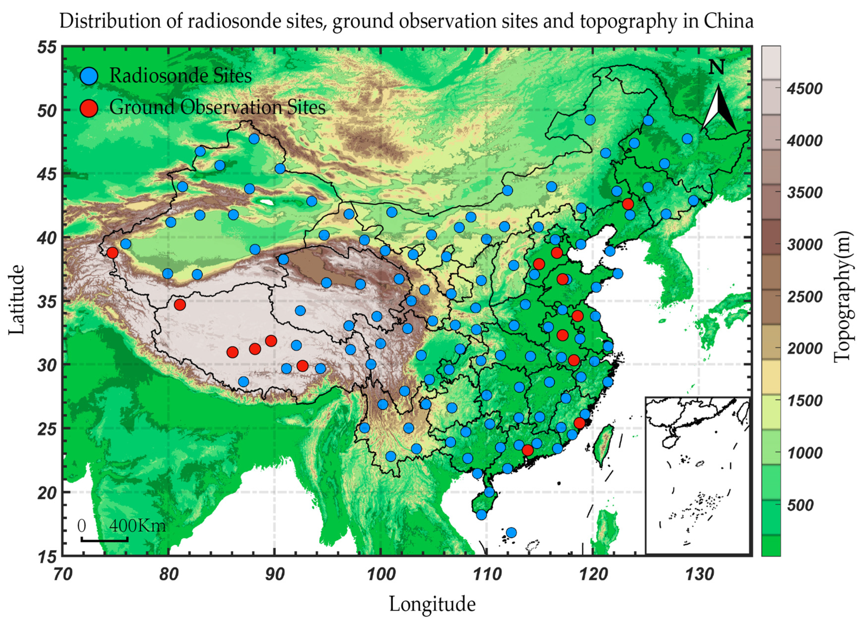
We used VHRS sounding data provided by the National Meteorological Information Center of China from 120 conventional sounding stations nationwide for the time period January 2019 to December 2020. Figure 1 shows that the distribution of sounding stations is both uniform and representative, except for the Qinghai–Tibetan Plateau. The sounding is carried out twice a day (at 0000 and 1200 UTC), and the data for meteorological elements (e.g., pressure, temperature, and wind speed) are detected via a GTS1 digital sounding instrument with a measurement frequency of about 1 s and a vertical resolution of about 4 m [28,29], In the data preprocessing, the original second-ordered coordinate data were quality controlled by using a low-pass filter, weighted least squares, and linear compensation methods to remove coordinate data disturbance caused by sounder swinging, radar measurement error, and atmospheric turbulence. Then, the vector average wind calculation method was adopted to obtain second-ordered wind speed and direction [30]. In addition, data with temperature, wind speed, or wind gradient anomalies and the adjacent data with a height difference greater than 100 m were deleted.

We used GPS occultation data from the COSMIC 2 [31], Metop A [32], Metop B, and Metop C satellites [33]. The GPS signal is in the microwave range and is therefore unaffected by clouds and precipitation [15]. Open-loop tracking technology and an advanced positioning system using the GPS, the Global Navigation Satellite System (GNSS), and a receiver system are used to improve the gain and signal quality for the detection of space weather [34]. GPS occultation data have a wider coverage and are more frequent in time than other satellite data. More than 90% of microwaves can penetrate 1 km above the ground, which is advantageous in research on the PBL. The four stars used in this study provide high-quality observations 7000 times/day.

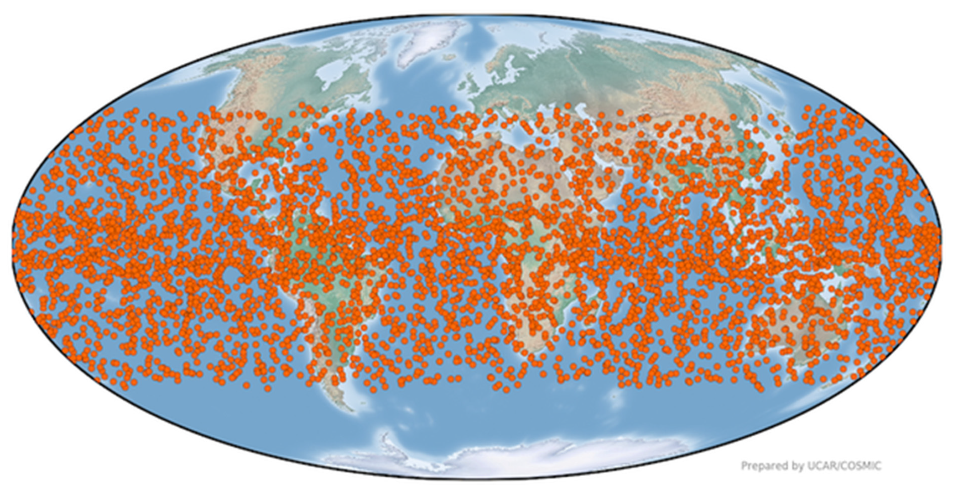
Figure 2 shows the distribution of data, which indicates that the GPS occultations are dense; so, they are good complements to the VHRS sounding data, especially at 0600 and 1800 UTC. The GPS occultation data record the air pressure, temperature, humidity, and refractive index with a vertical resolution of about 80 m. The GPS profiles contain a lot of valuable boundary layer information, which is vital for research in tropical and subtropical regions [35]. Data with a lowest detection height of <300 m were excluded to ensure data quality for the research on the PBLH in this paper.

The CMA-GFS model is an operational global forecast model developed independently by China (CMA is the abbreviation of China Meteorological Administration, and GFS is the abbreviation of Global Forecast System). It uses a nonhydrostatic [36], fully compressible set of equations with fully dynamical processes and a semi-implicit semi-Lagrangian [37] time integration scheme with two time layers: an Arakawa C grid in the horizontal direction [38] and a Charney–Phillips staggered grid in the vertical direction [39,40]. The physical parameterization schemes consist of the Rapid Radiative Transfer Model for the GCM (RRTMG) longwave and shortwave radiation schemes [41], the Simplified Arakawa Schubert (SAS) cumulus convection scheme [42,43], the New Medium Range Forecast (NMRF) boundary layer scheme [44,45], the Double Moment microphysics scheme, the Common Land Model (CoLM) [46] land surface scheme, and the gravity wave drag scheme [47]. The NMRF boundary layer scheme is the improved MRF scheme, adding the parameterization of the radiative cooling of stratocumulus clouds and strong entrainment at the top of the PBL. The experiments with the CMA-GFS showed that the simulations of stratocumulus clouds of NMRF were improved, and the vertical structures of the stratocumulus clouds were in better agreement with the observations, compared to the MRF scheme [44]. The horizontal resolution of the model is 25 km with 86 vertical layers. The model is integrated four times a day at 0000, 0600, 1200, and 1800 UTC and provides products at 3-h intervals.

We used the ERA5 global reanalysis dataset from the European Centre for Medium-Range Weather Forecasts (ECMWF) with a horizontal resolution of 25 km [48]. ERA5 reanalysis data are among the world’s highest-quality meteorological reanalysis data, which are often used to diagnose model biases, especially in regions lacking observations. Except for the sounding data and GPS data, we also compared the ERA5 dataset with the results from the CMA-GFS model to help explain the sources of bias in the PBLH predicted by the CMA-GFS model and also with the sounding data and GPS data to analyze the quality of ERA5.

2.2. PBLH Calculation Method

2.2.1. Bulk Richardson Method

The bulk Richardson method (referred to hereafter as the Ri method) is used in the CMA-GFS model and the ERA5 dataset to calculate the PBLH. The Ri is formulated using the following Equation (1):

$$Ri\left(n\right)=\frac{\frac{\mathrm{g}}{{\theta }_{vs}}\left({\theta }_{vn}-{\theta }_{vs}\right)\left(Z_n-Z_s\right)}{{\left(u_n-u_s\right)}^2+{\left(v_n-v_s\right)}^2+\left(b{u}_{*}^2\right)}$$

(1)

where Z is the height above the surface, the subscript n represents the meteorological element at the nth height, the subscript $s$ represents the surface, $g$ is the acceleration due to gravity, and θ_v is the virtual potential temperature. u,v are the horizontal velocity components, and $u_{*}$ is the surface friction velocity (negligible). b is a constant. Stull suggested that the height at which Ri reaches a threshold of 0.25 is the PBLH [1].

2.2.2. Potential Temperature Gradient Method

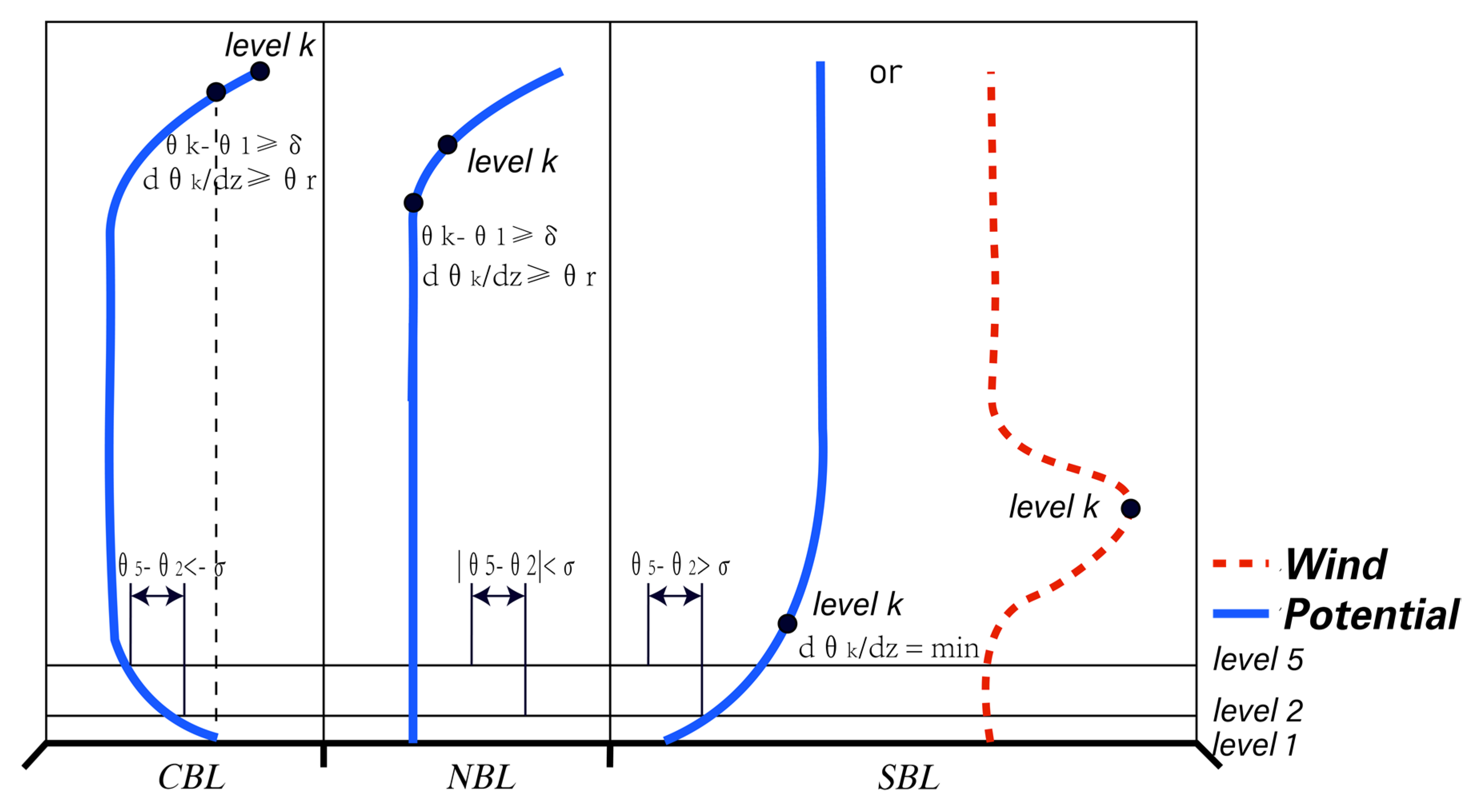
The PBLH was obtained by the potential temperature gradient method as a result of the lack of wind speed information in the GPS occultation data. This is also the most natural method to analyze the PBLH from sounding observations. The first step in the potential temperature gradient method is to determine the type of boundary layer from the thermodynamic point of view: a convective boundary layer (CBL), a stable boundary layer (SBL), or a neutral boundary layer NBL [33]. We used the method of Liu to determine the type of boundary layer and to calculate the PBLH [34] (Figure 3). The type of boundary layer is determined by Equation (2):

$$\begin{array}{c}{\theta }_5-{\theta }_2>\sigma \mathrm{stable}\\ |{\theta }_5-{\theta }_2|<\sigma \mathrm{natural}\\ {\theta }_5-{\theta }_2<-\sigma \mathrm{convective}\end{array}$$

(2)

where θ₅ and θ₂ are the potential temperatures at about 100 and 40 m above the surface, respectively, and $\sigma$ represents the critical threshold.

The PBLH of an SBL is determined at the height at which the rate of change of the potential temperature with height is at a minimum. However, in the presence of a low-level jet, the minimum of the top of the thermally stable layer and the center of the low-level jet is considered to be the PBLH.

The PBLH of a CBL and a NBL are both set as at the height at which the difference in the potential temperature between that height and the surface reaches a critical threshold δ, and the potential temperature gradient at that height meets the corresponding threshold θ_r:

$$\{\begin{array}{c}{\theta }_k-{\theta }_1>\delta \\ \mathsf{\Delta }\theta \equiv \frac{\partial \theta }{\partial z}\ge {\theta }_r\end{array}$$

(3)

Through field observations and extensive experimental studies, Liu (2010) set these thresholds as:

$$\{\begin{array}{c}\sigma =1K\\ \delta =0.5K\\ {\theta }_r=4K/m\end{array}$$

(4)

3. Results

3.1. Seasonal Bias of the PBLH in the CMA-GFS Model

The observed PBLH characteristics at 0000 and 1200 UTC in China have been analyzed by Guo [50], but the PBLH at 0600 and 1800 UTC have not been studied thoroughly, because there are few sounding data at these two times. We used occultation data to explore the characteristics of the PBLH in China at 0600 and 1800 UTC and compared these data with the model predictions. Since observation sites in China are uniformly spatially distributed (as shown in Figure 1 and Figure 2), and PBLH is a variable with good spatial continuity, we used the bicubic interpolation method to interpolate observations to the grid points of the model and compare them with the model.

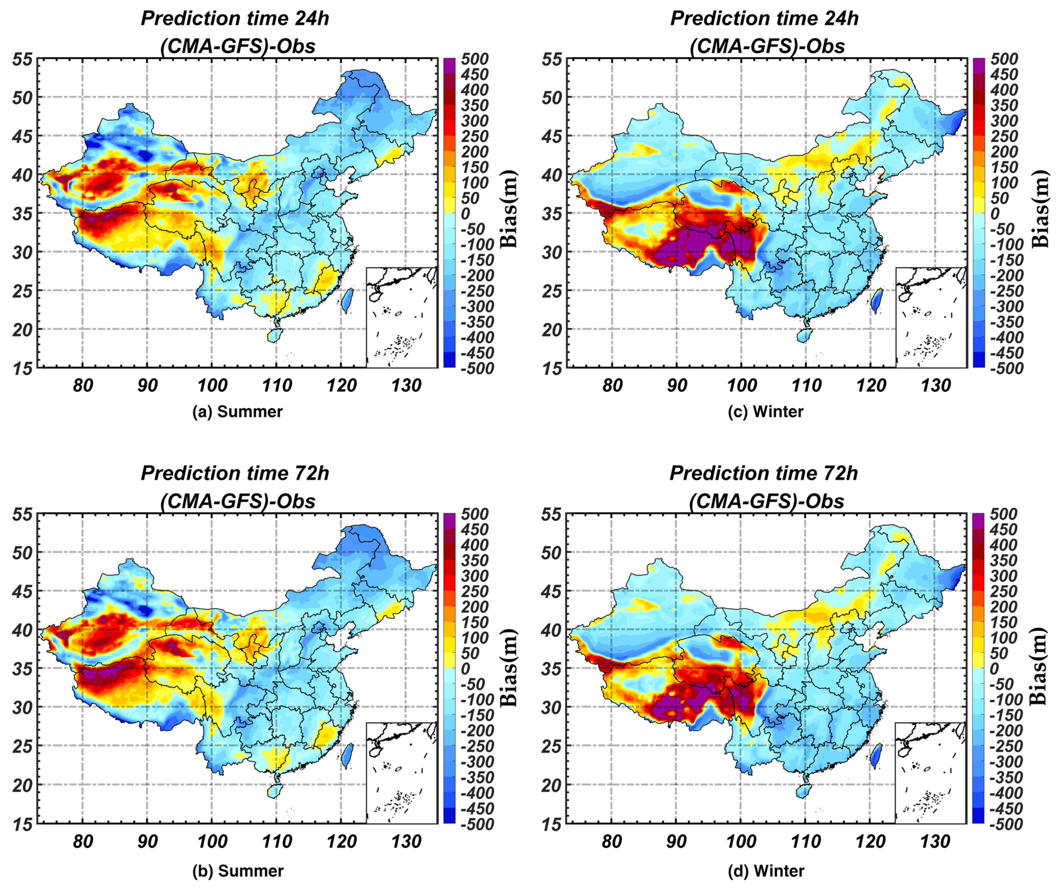
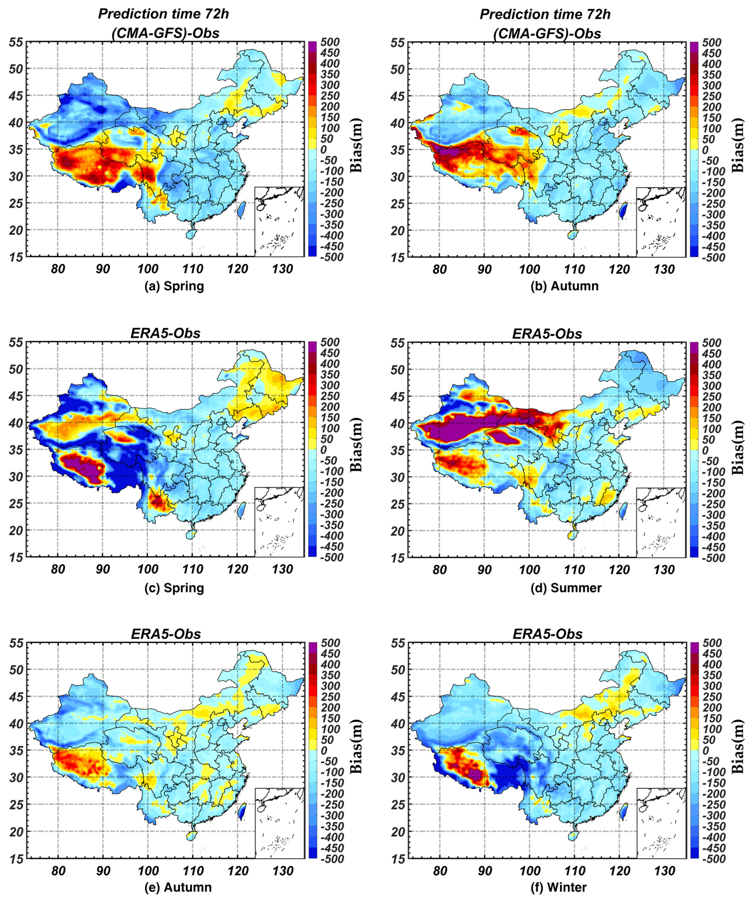
Figure 4 shows the daily average 24, 72 h bias of the PBLH in the CMA-GFS for winter and summer. The bias was almost uniformly negative in most of China in both winter and summer, except for the Qinghai–Tibetan Plateau. The maximum positive bias on the Qinghai–Tibetan Plateau occurred over the northern plateau in summer but over the southern plateau in winter. When the integration moved forward from 24 to 72 h, the positive bias in the eastern Qinghai–Tibetan Plateau extended slightly to the south in summer, because this area is a heat source with a large sensible heat flux throughout the year, which contributes to the large bias of the model and gradually accumulates with the integration time. However, the main pattern of the model bias did not change from the 24 to 72 h forecasts at any time of year (Figure 4a and Figure 5b). We therefore focused on the 72 h model forecast.

Figure 4 and Figure 5a,b show that the bias of the PBLH in the CMA-GFS model also had little seasonal variation. The main model bias was an underestimation in East China, with an average bias of about −100 m. There was an overestimation on the Qinghai–Tibetan Plateau, with an average bias of about 400 m. The annual variation of the amplitude and coverage of the bias in the PBLH in East China and the Qinghai–Tibetan Plateau were small, and their specific causes are analyzed in the following section.

There was a thin line of negative bias following the topography in the southern Tarim Basin, probably due to the large slope in this area, but this bias could not be confirmed as a result of the paucity of observations in this region. However, bias in the pressure forecast over this complex topography might directly affect the calculation of the potential temperature and contribute to the bias.

The ERA5 reanalysis dataset showed similar distributions of bias to the CMA-GFS model. The pattern of the bias also changed little with the season and was systematically underestimated in East China and overestimated in the western Tibetan Plateau. In contrast, the bias of the CMA-GFS model and the ERA5 dataset were the opposite in the eastern Tibetan Plateau (28–35° N, 90–100° E). The ERA5 dataset showed an underestimate with a bias of about −500, whereas the bias in the CMA-GFS model was an overestimate of about 500 m. The temporal and spatial distribution of the ERA5 bias was similar to those of the CMA-GFS model, which proves that the bias in the CMA-GFS model may not have been caused by the initial data. We explain the reasons for the bias in the CMA-GFS model in the following section.

3.2. Diurnal Bias of the PBLH in the CMA-GFS Model

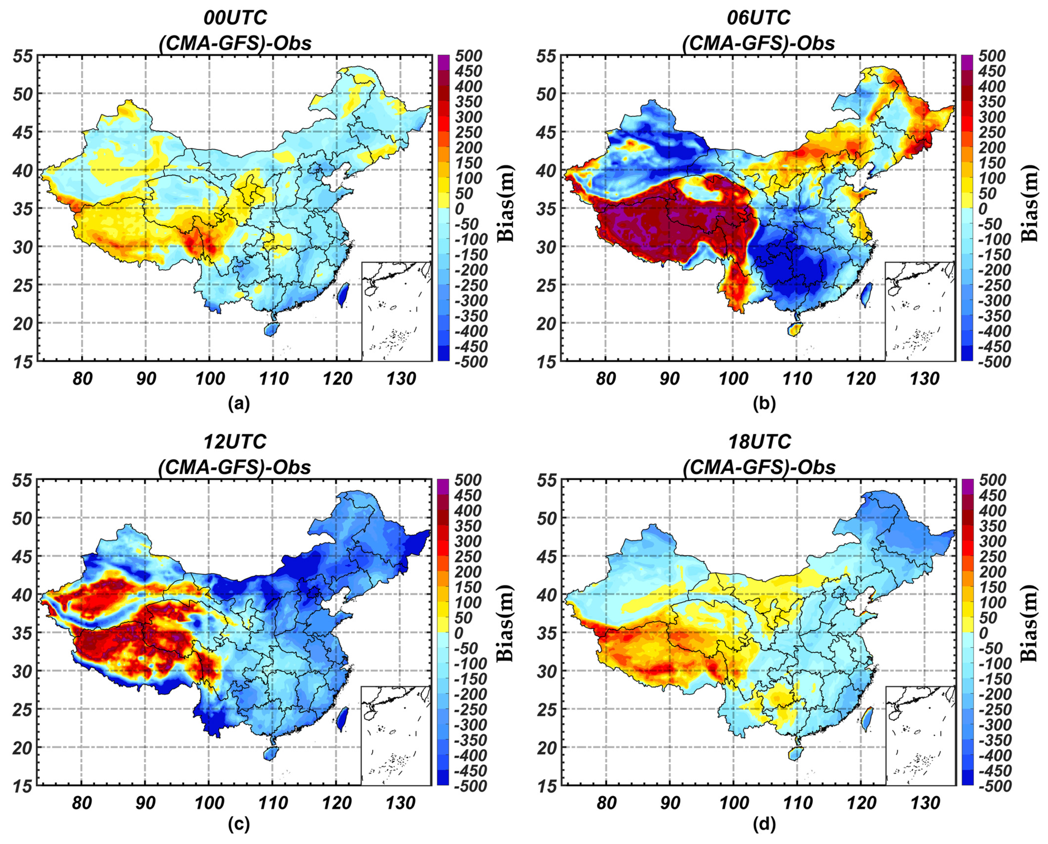
Figure 6 shows that the PBLH bias in the CMA-GFS model exhibited a clear diurnal cycle. The negative bias of the model peaked at 0600 and 1200 UTC, when East China was at the peak of turbulence development. The observations tended to show a higher PBLH at 0600 and 1200 UTC, but the model did not develop the PBL to the corresponding height. Although the amplitudes of the bias changed with time, the coverage did not change very much. At 0600 and 1200 UTC, the PBL is prone to be unstable and convection is active, the PBLH is at height of the lifting condensation level (LCL). Therefore, the obvious underestimation of PBLH at 0600 and 1200 UTC might be caused by underestimation of LCL in CMA-GFS, which implies the need for improvement of the convection scheme in the future.

The positive bias of the model also reached >500 m over the Tibetan Plateau at 0600 and 1200 UTC. The PBLH should develop at a higher level as a result of the solar radiation and the roughness of the underlying surface of the Tibetan Plateau. During this period, the main contributions are from the thermal effect, because the strong turbulence mixes the momentum thoroughly in the vertical direction, which means that the wind shear effect is small. However, we found that the CMA-GFS model predicted a stronger wind shear than the observations, which drove the development of a deeper PBL in the CMA-GFS model.

3.3. Different Underlying Surface

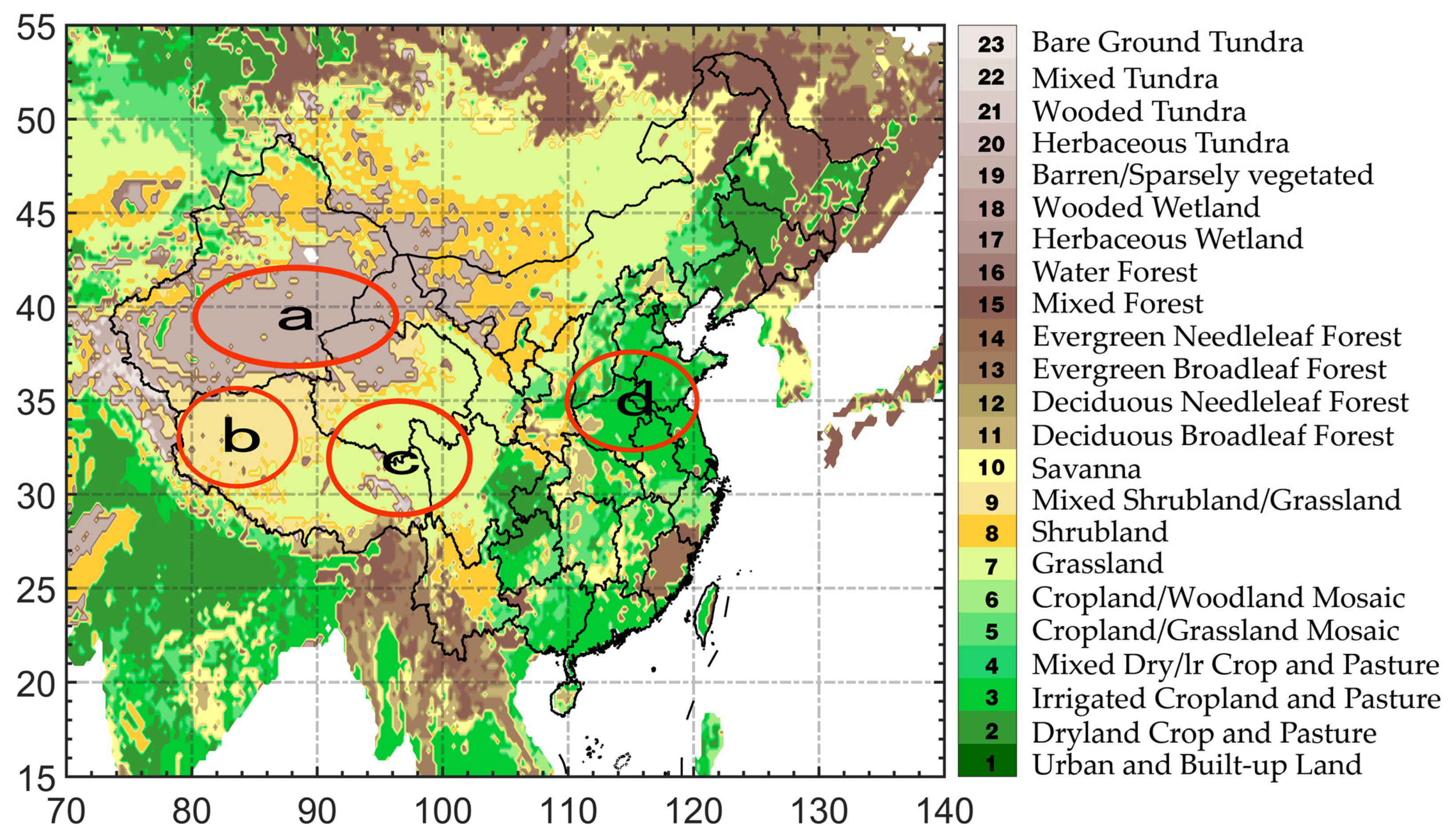
Different underlying surfaces have a significant influence on the development of the boundary layer [17]. We selected four surface types representative of the underlying surfaces in China as prescribed in the CMA-GFS model: barren and sparse vegetation; mixed shrubland and grassland; highland grasslands; and irrigated cropland and pasture (Figure 7).

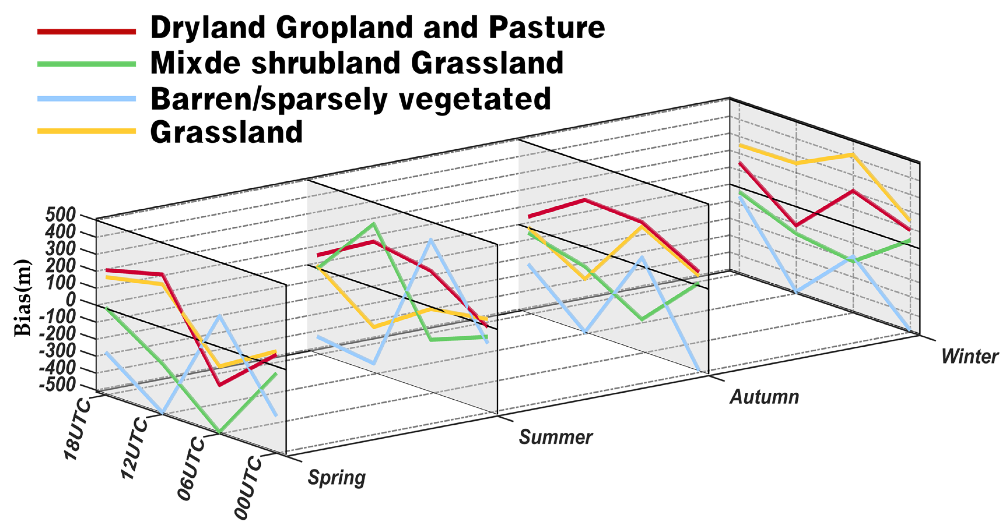
Figure 8 shows that the biases of the model were more prominent in mixed shrubland and grassland, with positive bias throughout the year ranging from 0 to 200 m. In the barren and sparse vegetation area, there was an overestimation at 1200 UTC in summer and an underestimation at all other times and seasons by a maximum of −500 m at 0600 UTC in spring, when the development of turbulence was at its peak. In addition, the bias of up to 200 m tended to be more evident in the highland grassland areas in winter. The model underestimated the PBLH in irrigated cropland and pasture areas, with a maximum of more than −500 m in winter but overestimated the PBLH at 0600 UTC in spring and summer.

Barren areas and areas with sparse vegetation have smooth lower boundaries and a small specific heat capacity, which means that they have a strong wind shear and heat flux, and a high PBLH is easily developed [51,52], although the model showed negative bias. The mixed shrubland and grassland and grasslands have a large specific heat capacity and rough lower boundaries, which leads to a small sheer and, therefore, a low PBLH. Nonetheless, the model showed a large positive bias, because it had a significant bias in the sensible heat flux and wind shear compared with the observations.

4. Discussion

4.1. Evaluation of the Model Bias

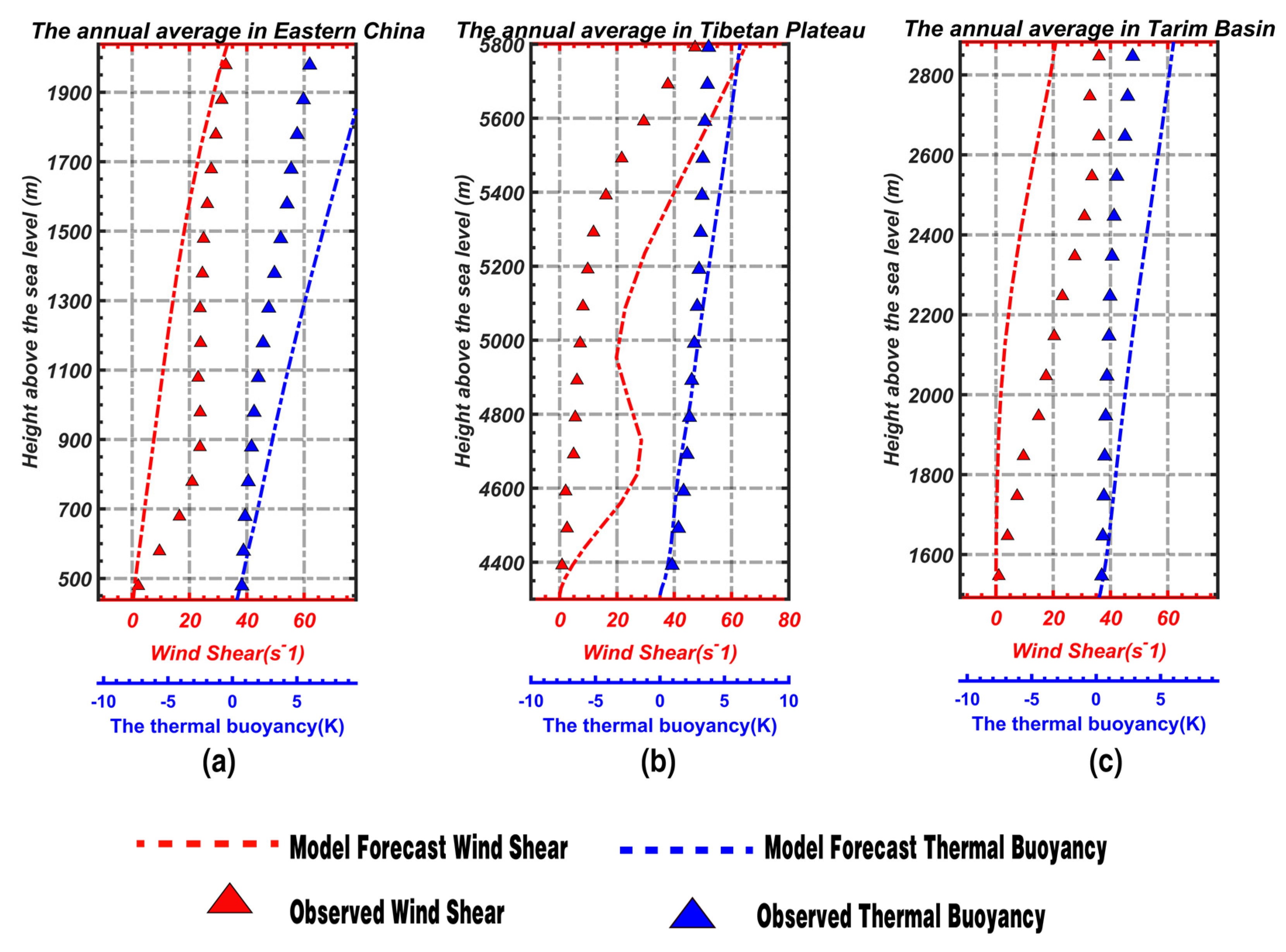
This section aims to determine the causes of the model bias by analyzing the crucial variables affecting the PBLH, such as wind shear, buoyancy, and the sensible heat flux. The factors directly impacting the PBLH are the wind shear ($W_s$) and the thermal buoyancy (T_b) from Equation (1). $W_s$ is calculated as:

$$Ws={\left(u_h-u_s\right)}^2+{\left(v_h-{\mathrm{v}}_s\right)}^2$$

(5)

where u represents the latitudinal wind speed, v represents the longitudinal wind speed, subscript h represents different heights, and subscript s represents the surface. Equation (1) shows that the larger the wind shear, the higher the PBLH.

Thermal buoyancy (considering the influence of water vapor) T_b is calculated as:

$$Tb={\theta }_v-{\theta }_{vs}$$

(6)

where θ_v is the virtual potential temperature, and subscript s represents the surface. A larger $T_b$ corresponds to a more stable air mass, leading to weak development of the PBL.

4.2. Bias in East China

The CMA-GFS model mainly underestimated the PBLH in East China. Figure 9a compares the dynamical (wind shear) and thermal effects averaged over East China by the CMA-GFS model with the observations. The Ws of the model was significantly lower than the observations, and the $Tb$ of the model was larger than the observations. As shown in Section 4.1, both smaller Ws and a larger TB led to the development of a lower boundary layer height. Discovered from dynamical and thermal effects, the small vertical wind shear and larger thermal buoyancy were, therefore, direct reasons for the systematic underestimation of the PBLH in East China by the CMA-GFS model.

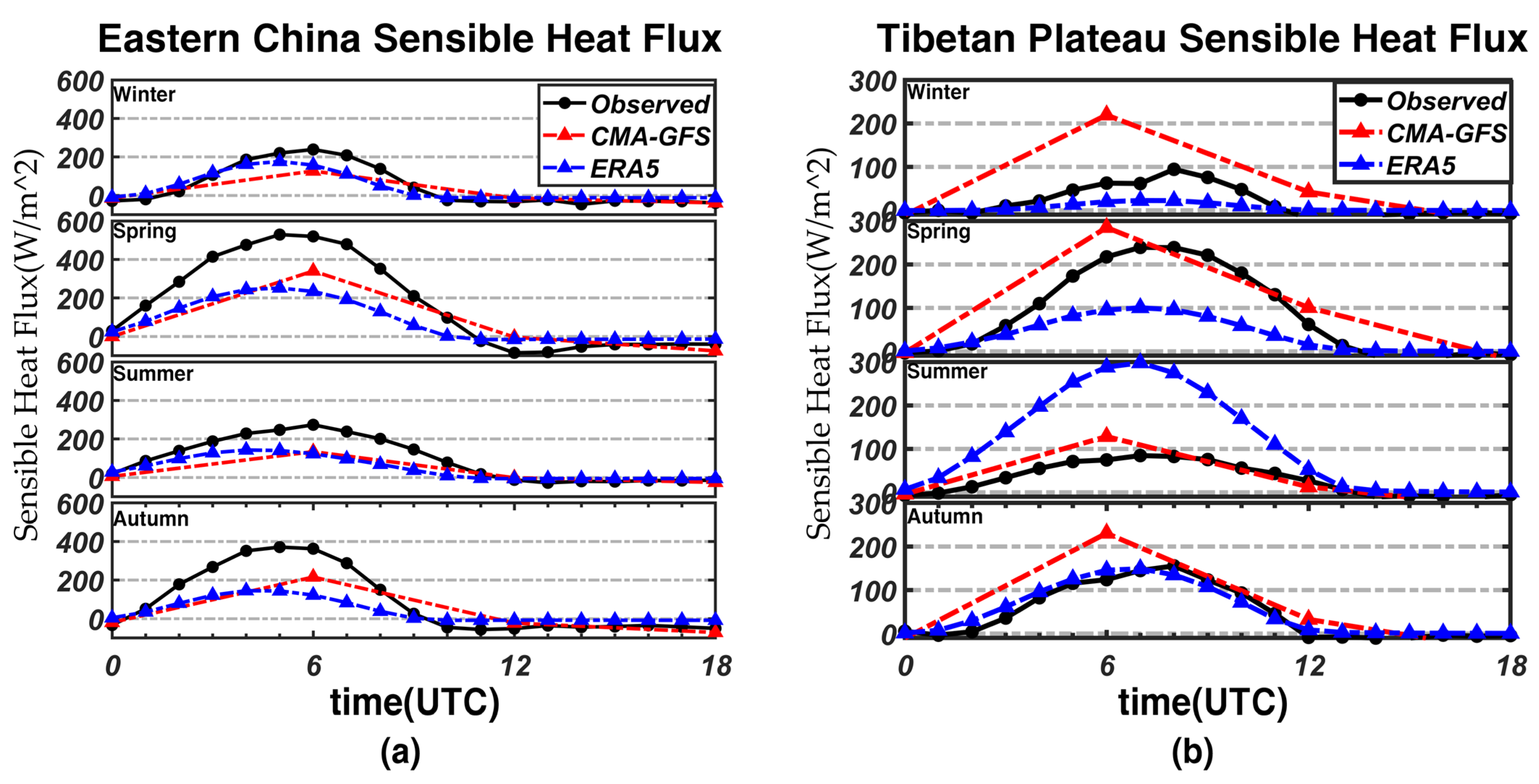
The surface heat flux determines the heat exchange near the interface, affecting the temperature near the surface. Meanwhile, the sensible heat flux is the source of energy for the development of meteorological elements of the boundary layer and is, therefore, closely related to the boundary layer height. The seasonal average sensible heat flux at nine eastern observational stations, including Haihe, Changling, and Dinghushan stations (Figure 1), were compared with the sensible heat flux predicted by the CMA-GFS model and the ERA5 dataset. These data were provided by FluxNet (FLUXNET) and the National Qinghai-Tibet Plateau Data Center (National Qinghai-Tibet Plateau Scientific Data Center, tpdc.ac.cn) [53]. Figure 10a shows that the sensible heat flux forecast by the CMA-GFS model and the ERA5 dataset was consistently lower than the observations in East China. The bias changed little with the season but did change noticeably with the diurnal cycle. The sensible heat fluxes in the CMA-GFS model had a significant negative bias at 0600 UTC, with a maximum of 150 W/m. This led to smaller surface heating and ground thermal effects than in the observations, resulting in underestimation of the PBLH.

The sensible heat flux was calculated using the near-surface layer parameterization scheme in the CMA-GFS model and the ERA5 dataset:

$$J_s=\rho C_H{|\mathrm{U}}_n{\left|\right(\mathrm{c}}_p{\mathrm{T}}_n{-\mathrm{c}}_p{\mathrm{T}}_{surf})$$

(7)

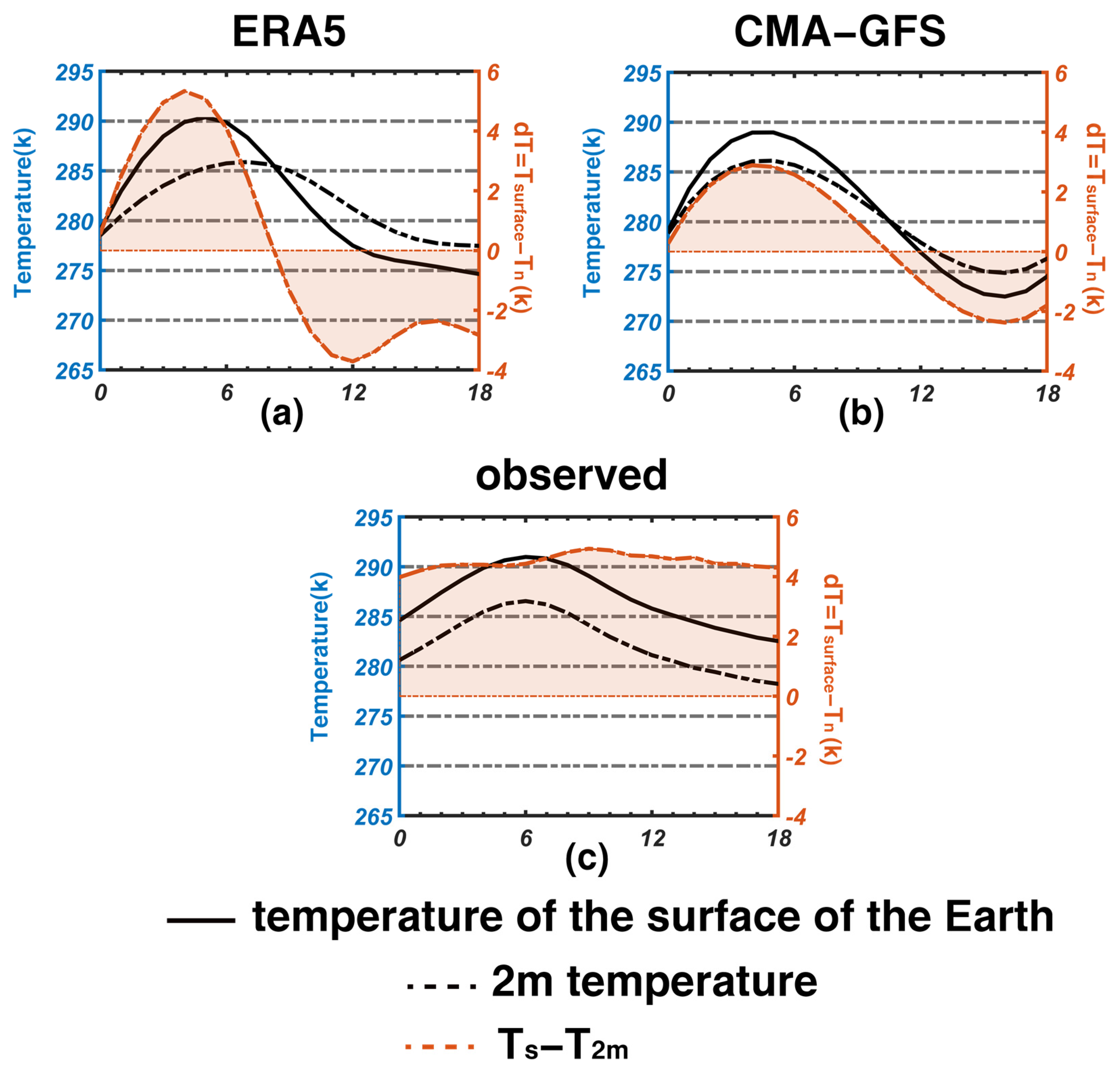
where J_s is the sensible heat flux, ρ is the density, C_H is the heat exchange coefficient, U is the wind speed, C_p is the constant pressure specific heat capacity, T. represents the temperature, and the subscripts s and surf mean at the lowest model level (about 10 m) and surface layer, respectively. Because there is no 10 m temperature data in the CMA-GFS model and the ERA5 dataset, the difference between the 2 m temperature and the surface temperature were compared between the CMA-GFS model and the observations. The difference between the surface temperature and the 2 m temperature is expressed by:

$$dT=Ts-T_{2m}$$

(8)

where T_s is the surface temperature, T_2m is the temperature 2 m above the surface, dT is the difference in temperature between them, and subscript s represents the surface. The larger the value of dT, the stronger the upward transfer of heat from the surface, which has a positive effect on the sensible heat flux. Figure 11 shows that both the CMA-GFS model and ERA5 are in good agreement with the observation for T2m but significantly underestimated T_s and, thus, dT, which is why the both CMA-GFS and ERA5 underestimated the sensible heat flux. CMA-GFS and ERA5 showed a similar bias producing mechanism, i.e., underestimation of T_s leads to underestimation of sensible heat flux and, then, PBLH. This means that the mechanism explaining the biases in PBLH in East China is reliable. T_s is calculated through surface energy balance equation, which is decided by net shortwave and longwave radiation fluxes and turbulent sensible and latent heat fluxes at the surface. From Figure 11, underestimation of T_s was uniform during the day and at night; so, shortwave radiation fluxes may be not the reason, since there are no shortwave radiation fluxes at night. Therefore, the underestimation of T_s and sensible heat flux might be related to biases in longwave radiation fluxes and latent heat fluxes, which means that the surface layer scheme and longwave radiation parameterization in the model should be improved in the future.

4.3. Bias over the Qinghai–Tibetan Plateau and in the Tarim Basin

Both the CMA-GFS model and the ERA5 dataset showed significant bias over the Qinghai–Tibetan Plateau. It is difficult to evaluate these biases because of the complex topography and limited observational data for the Tibetan Plateau. Only a preliminary analysis could be conducted based on the available information.

We analyzed the direct factors affecting the PBLH. Figure 9b shows that the annual average Ws in the model was larger than the observations, and thewas smaller than the observations. The stronger Ws and weaker TB enabled the PBL to develop at a higher level. The wind shear and buoyancy factors therefore led directly to a deeper PBL and considerable forecast bias in the model.

The sensible heat fluxes were evaluated using data from six stations on the Tibetan Plateau. Figure 10b shows that the sensible heat flux forecast by the CMA-GFS model was stronger than the observations throughout the year. The overestimate was larger in winter and smaller in summer and was larger in the afternoon and evening but smaller at night and in the early morning. This corresponded to the seasonal and daily changes in the bias of the PBLH over the Tibetan Plateau. The model overestimated the sensible heat flux over the Tibetan Plateau during the daytime (0600–1200 UTC) and superimposed stronger forecasts of wind shear. This means that the model obtained better conditions to develop a deeper PBL than the observation, with the bias reaching >500 m during the daytime. As shown in Figure 10b, there was agreement between the ERA5 and the observations for sensible heat fluxes in autumn; therefore, it can be found from Figure 5e that the bias of ERA5 in autumn was smaller in the Qinghai-Tibet Plateau. This indicates that the sensible heat flux is critical for boundary layer prediction. So, the analyses over the Qinghai–Tibetan Plateau also imply a need to improve the surface layer scheme in CMA-GFS.

The underlying surface properties of the desert in the Tarim Basin mean that the thermal effect is the primary driver for the development of the PBLH [54]. The model underestimated the buoyancy but had a similar wind shear to the observations, which stabilized the boundary layer and favored the development of a lower PBL (Figure 9c). We can only tentatively conclude that the weak buoyancy effect was one of the reasons for the underestimation of the PBLH in this area as a result of the lack of flux observations in this region.

This analysis shows that the main reasons for the overestimation of the PBLH over the Qinghai–Tibetan Plateau were the simultaneously strong wind shear and sensible heat flux in the model. There were many factors responsible for the bias in the PBLH over the Qinghai–Tibetan Plateau, and the contributions from each factor were more significant than those in other regions.

5. Conclusions

This study of the PBLH in China based on VHRS and GPS occultation data has shown that: the CMA-GFS model underestimated the PBLH in East China. The size of the underestimation did not change much seasonally, but there was a diurnal cycle with a maximum bias of about −500 m at 0600 UTC. The model showed an overestimation over the Qinghai–Tibetan Plateau. The bias reached a maximum of about 500 m at 0600 UTC and covered the whole Qinghai–Tibetan Plateau at this time.

VHRS and flux station data were used to evaluate the bias in the PBLH predicted by the CMA-GFS model and to analyze the thermal and dynamical factors for the development of the PBLH. Our conclusions are as follows.

The underestimation of the PBLH in East China was the combined result of an underestimation of the wind shear and sensible heat flux, which restricts the development of the PBL. The smaller sensible heat flux has the greatest effect on preventing the upward growth of the PBL.

The bias in the overestimation over the Tibetan Plateau was mainly the result of the stronger wind shear and sensible heat flux. They collectively drove the model to develop a deeper PBL, producing a significant positive bias of the PBLH. The bias was more apparent at 0600 and 1200 UTC during the daytime than during the night, mainly due to the combined effects of a strong sensible heat flux with the overestimated wind shear and underestimated buoyancy.

The bias in the predicted PBLH had a significant diurnal cycle, mainly due to the large variations in the amplitude of the bias in the sensible heat flux over time. The bias in the sensible heat flux reached a maximum at 0600 UTC and, then, started to decrease at 12UTC, causing the PBLH to vary with the same pattern.

The PBLH biases of the CMA-GFS model are caused by many meteorological factors, so, the accurate prediction of it is difficult. This study indicates that in addition to optimizing the BL scheme to improve the transport of heat and momentum fluxes, the convection, surface layer scheme, and longwave radiation parameterization in the model also should be improved in the future to improve the prediction of PBLH.

The results of this study will help to understand the reasons for the bias in PBL of the CMA-GFS model and help to improve the model. However, due to the limitations of the data, our current work only evaluated some meteorological variables and did not evaluate the important physical quantities in the boundary layer parameterization scheme, such as the turbulent exchange coefficient, etc.; so, the analyses are preliminary. In future studies, we will evaluate the turbulent exchange coefficient, based on the observation study we have just finished, and physical processes such as heat, momentum, and turbulence transport to progressively refine the evaluation of the model. This work will play an important role in improving the model.

References

- Stull, R.B. An Introduction to Boundary Layer Meteorology; Kluwer Academic Publishers: Dordrecht, The Netherlands, 1988; pp. 1–545. [Google Scholar]
- Cheng, S.Y.; Zhang, B.N.; Bai, T.X. Study on the height of atmospheric mixed layer and its meteorological characteristics in Beijing. J. Environ. Eng. 1992, 46, 52. (In Chinese) [Google Scholar]
- Suarez, M.J.; Arakawa, A.; Randall, D.A. The parameterization of the planetary layer in the UCLA general circulation model: Formulation and results. Mon. EeaRev. 1983, 111, 2224–2243. [Google Scholar] [CrossRef] [Green Version]
- Konor, C.S.; Boezio, G.C.; Mechoso, C.R.; Arakawa, A. Parameterization of PBL Processes in an Atmospheric General Circulation Model: Description and Preliminary Assessment. Mon. Weather Rev. 2009, 137, 1061–1082. [Google Scholar] [CrossRef] [Green Version]
- Ren, Y.; Zhang, H.; Wei, W.; Cai, X.; Song, Y.; Kang, L. A study on atmospheric turbulence structure and intermittency during heavy haze pollution in the Beijing area. Sci. China Earth Sci. 2019, 62, 2058–2068. [Google Scholar] [CrossRef]
- Garrat, J.R. The Atmospheric Boundary Layer; Cambridge University Press: Cambridge, UK, 1992. [Google Scholar]
- Vilà-Guerau de Arellano, J.; Van Heerwaarden, C.C.; Van Stratum, B.J. Atmospheric Boundary Layer: Integrating Air Chemistry and Land Interactions; Cambridge University Press: Cambridge, UK, 2015. [Google Scholar]
- Zhong, J.T.; Zhang, X.Y.; Wang, Y.Q. Relative contributions of boundary-layer meteorological factors to the explosive growth of PM2.5 during the red-alert heavy pollution episodes in Beijing in December 2016. J. Meteor. Res. 2017, 31, 809–819. [Google Scholar] [CrossRef]
- Liu, H.Z.; Wang, L.; Du, Q. An overview of recent studies on atmospheric boundary layer physics (2012–2017). Chin. J. Atmos. Sci. 2018, 42, 823–832. (In Chinese) [Google Scholar] [CrossRef]
- Yang, F.Y. Comparison of Determination Methods and Characteristics of Boundary Layer Height in Semi-Arid Area; Lanzhou University: Lanzhou, China, 2018. (In Chinese) [Google Scholar]
- Gui, K.; Che, H.Z.; Wang, Y.Q.; Wang, H. Satellite-derived PM2.5 concentration trends over Eastern China from 1998 to 2016: Relationships to emissions and meteorological parameters. Environ. Pollut. 2019, 247, 1125–1133. [Google Scholar] [CrossRef]
- Zhang, H.S.; Zhang, X.Y.; Li, Q.H. Research progress on estimation of atmospheric boundary layer height. Acta Meteorol. Sin. 2020, 78, 522–536. (In Chinese) [Google Scholar] [CrossRef]
- Wang, Z.; Cao, X.; Zhang, L.; Notholt, J.; Zhou, B.; Liu, R.; Zhang, B. Lidar measurement of planetary boundary layer height and comparison with microwave profiling radiometer observation. Atmos. Meas. Tech. 2012, 5, 1965–1972. [Google Scholar] [CrossRef] [Green Version]
- Saeed, U.; Rocadenbosch, F.; Crewell, S. Adaptive Estimation of the Stable Boundary Layer Height Using Combined Lidar and Microwave Radiometer Observations. IEEE Trans. Geosci. Remote Sens. 2016, 54, 6895–6906. [Google Scholar] [CrossRef] [Green Version]
- Bravo-Aranda, J.A.; de Arruda Moreira, G.; Navas-Guzmán, F.; Granados-Muñoz, M.J.; Guerrero-Rascado, J.L.; Pozo-Vázquez, D.; Arbizu-Barrena, C.; Olmo Reyes, F.J.; Mallet, M.; Alados Arboledas, L. A new methodology for PBL height estimations based on lidar depolarization measurements: Analysis and comparison against MWR and WRF model-based results. Atmos. Chem. Phys. 2017, 17, 6839–6851. [Google Scholar] [CrossRef] [Green Version]
- Emeis, S.; Schäfer, K.; Münkel, C. Surface-based remote sensing of the mixinglayer height-A review. Meteorol. Z. 2008, 17, 621–630. [Google Scholar] [CrossRef] [PubMed]
- Kallistratova, M.A.; Petenko, I.V.; Kouznetsov, R.D.; Kulichkov, S.N.; Chkhetiani, O.G.; Chunchusov, I.P.; Lyulyukin, V.S.; Zaitseva, D.V.; Vazaeva, N.V.; Perepelkin, V.G.; et al. Sodar Sounding of the Atmospheric Boundary Layer: Review of Studies at the Obukhov Institute of Atmospheric Physics, Russian Academy of Sciences. Izv. Atmos. Ocean. Phys. 2018, 54, 242–256. [Google Scholar] [CrossRef]
- Liang, Z.H.; Wang, D.H.; Liang, Z.M. Spatio-temporal characteristics of boundary layer height Derived from Soundings. J. Appl. Meteorol. Sci. 2020, 31, 447–459. (In Chinese) [Google Scholar]
- Ao, C.O.; Waliser, D.E.; Chan, S.K. Planetary boundary layer heights from GPS radio occultation refractivity and humidity profiles, J. Geophys. Res. 2012, 117, D16117. [Google Scholar] [CrossRef] [Green Version]
- Liu, Y.; Tang, N.J.; Yang, X.S. Height of atmospheric boundary layer top as detected by COSMIC GPS radio occultation data. J. Trop. Meteorol. 2015, 31, 43–50. (In Chinese) [Google Scholar]
- Angevine, W.M.; White, A.B.; Avery, S.K. Boundary-layer depth and entrainment zone characterization with a boundary-layer profiler. Bound.-Layer Meteorol. 1994, 68, 375–385. [Google Scholar] [CrossRef]
- Hu, M.B.; Zheng, G.G.; Zhang, P.C. The study of maximum entropy method user in wind profiler. Spectrosc. Spectr. Anal. 2012, 32, 1085–1089. (In Chinese) [Google Scholar]
- Ge, S.R.; Hu, N. Research on vertical air velocity and planetary boundary height detection by the wind profiler. Natl. Univ. Def. Technol. 2017 000916. (In Chinese) [Google Scholar]
- Sokolovskiy, S.V.; Rocken, C.; Lenschow, D.H.; Kuo, Y.-H.; Anthes, R.A.; Schreiner, W.S.; Hunt, D.C. Observing the moist troposphere with radio occultation signals from COSMIC. Geophys. Res. Lett. 2007, 34, L18802. [Google Scholar] [CrossRef] [Green Version]
- Seibert, P.; Beyrich, F.; Gryning, S.-E.; Joffre, S.; Rasmussen, A.; Tercier, P. Review, and intercomparison of operational methods for the determination of the mixing height. Atmos. Environ. 2000, 34, 1001–1027. [Google Scholar] [CrossRef]
- Holtslag, A.A.; Nieuwstadt, F.T. Scaling the atmospheric boundary layer Boundary-Layer Meteorol. Bound.-Layer Meteorol. 1986, 36, 201–209. [Google Scholar] [CrossRef]
- Su, T.N.; Li, Z.Q. Relationships between the planetary boundary layer height and surface pollutants derived from lidar observations over China: Regional pattern and influencing factors. Atmos. Chem. Phys. 2018, 18, 15921–15935. [Google Scholar] [CrossRef] [Green Version]
- Wu, H.K.; Chen, Q.Y.; Hua, W. A statistical study of Gravity Wave with Second-Level Radiosonde Data in Sichuan. J. Appl. Meteorol. Sci. 2019, 30, 491–501. (In Chinese) [Google Scholar]
- Li, F.F.; Chen, Q.Y.; Wu, H.K. A statistical study of Brunt-Vaisala frequency with Second-Level Radiosonde Data in China. J. Appl. Meteorol. Sci. 2019, 30, 629–640. (In Chinese) [Google Scholar]
- Chen, W.; Li, Y. Statistical Relationship between Gravity Waves over the Eastern Tibetan Plateau and the Southwest Vortex. Chin. J. Atmos. Sci. 2019, 43, 773–782. (In Chinese) [Google Scholar]
- Tsai, L.C.; Su, S.Y. Ionospheric electron density profiling and modeling of COSMIC follow-on simulations. J. Geod. 2016, 90, 129–142. [Google Scholar] [CrossRef]
- Hautecoeur, O.; Borde, R. Derivation of wind vectors from AVHRR/Metop at EUMETSAT. J. Atmos. Ocean. Technol. 2017, 34, 1645–1659. [Google Scholar] [CrossRef]
- Yan, B.; Chen, J.; Zou, C.-Z. Calibration and Validation of Antenna and Brightness Temperatures from Metop-C Advanced Microwave Sounding Unit-A (AMSU-A). Remote Sens. 2020, 12, 2978. [Google Scholar] [CrossRef]
- Ho, S.P.; Zhou, X.; Shao, X.; Zhang, B. Initial Assessment of the COSMIC-2/FORMOSAT-7 Neutral Atmosphere Data Quality in NESDIS/STAR Using In Situ and Satellite Data. Remote Sens. 2020, 12, 4099. [Google Scholar] [CrossRef]
- Ho, S.-P.; Peng, L.; Mears, C.; Anthes, R.A. Comparison of Global Observations and Trends of Total Precipitable Water Derived from Microwave Radiometers and COSMIC Radio Occultation from 2006 to 2013. Atmos. Chem. Phys. 2018, 18, 259–274. [Google Scholar] [CrossRef] [Green Version]
- Li, X.; Peng, X.; Li, X. An improved dynamic core for a non-hydrostatic model system on the Yin-Yang grid. Adv. Atmos. Sci 2015, 32, 648–658. [Google Scholar] [CrossRef]
- Yang, X.; Chen, J.; Hu, J.; Chen, D.; Shen, X.; Zhang, H. A semi-implicit semi-Lagrangian global nonhydrostatic model and the polar discretization scheme. Sci. China Ser. D-Earth Sci. 2007, 50, 1885–1891. [Google Scholar] [CrossRef]
- Ma, Z.; Liu, Q.; Zhao, C.; Shen, X.; Wang, Y.; Jiang, J.H.; Li, Z.; Yung, Y. Application and evaluation of an explicit prognostic cloud-cover scheme in GRAPES global forecast system. J. Adv. Modeling Earth Syst. 2018, 10, 652–667. [Google Scholar] [CrossRef]
- Charney, J.G.; Phillips, N.A. Numerical integration of the quasi-geostrophic equations for barotropic and simple baroclinic flows. J. Meteorol. 1953, 10, 71–99. [Google Scholar] [CrossRef] [Green Version]
- Chen, J.; Ma, Z.; Li, Z.; Shen, X.; Su, Y.; Chen, Q.; Liu, Y. Vertical diffusion and cloud scheme coupling to the Charney–Phillips vertical grid in GRAPES global forecast system. Q. J. R. Meteorol. Soc. 2020, 146, 2191–2204. [Google Scholar] [CrossRef]
- Morcrette, J.-J.; Barker, H.W. Impact of a new radiation package, McRad, in the ECMWF Integrated Forecast System. Mon. Weather Rev. 2008, 136, 4773–4798. [Google Scholar] [CrossRef]
- Arakawa, A.; Schubert, W.H. Interaction of a cumulus cloud ensemble with the large-scale environment, Part I. J. Atmos. Sci. 1974, 31, 674–701. [Google Scholar] [CrossRef] [Green Version]
- Liu, K.; Chen, Q.; Sun, J. Modification of cumulus convection and planetary boundary layer schemes in the GRAPES global model. J. Meteorol. Res. 2015, 29, 806–822. [Google Scholar] [CrossRef]
- Hong, S.Y.; Pan, H.L. Nonlocal boundary layer vertical diffusion in a medium-range forecast model. Mon. Weather Rev. 1996, 124, 2322–2339. [Google Scholar] [CrossRef] [Green Version]
- Han, J.; Pan, H.L. Revision of convection and vertical diffusion schemes in the NCEP global forecast system. Wea. Forecast. 2011, 26, 520–533. [Google Scholar] [CrossRef]
- Dai, Y.; Zeng, X. The Common Land Model, B. Am. Meteorol. Soc. 2003, 84, 1013–1023. [Google Scholar] [CrossRef] [Green Version]
- Chen, Q.Y.; Shen, X.S. Momentum Budget Diagnosis and the Parameterization of Subgrid-Scale Orographic Drag in Global GRAPES. J. Meteorol. Res. 2016, 30, 771–788. [Google Scholar] [CrossRef]
- Hersbach, H.; Bell, B.; Berrisford, P.; Hirahara, S.; Horanyi, A.; Muñoz-Sabater, J.; Nicolas, J.; Peubey, C.; Radu, R.; Schepers, D.; et al. The ERA5 global reanalysis. Q. J. R. Meteor. Soc. 2020, 146, 1999–2049. [Google Scholar] [CrossRef]
- Liu, S.Y.; Liang, X. Observed Diurnal Cycle Climatology of Planetary Boundary Layer Height. J. Clim. 2010, 23, 5790–5809. [Google Scholar] [CrossRef]
- Guo, J.P.; Miao, Y.C. The climatology of planetary boundary layer height in China derived from radiosonde and reanalysis data. Atmos. Chem. Phys. 2016, 16, 13309–13319. [Google Scholar] [CrossRef] [Green Version]
- Li, Y.; Zhang, Q.; Zhang, A.; Chen, Y.; Yang, M. Analysis on Atmosphere Boundary Layer Variation Characteristics and Their Impact Factors in Arid Region and Semi-Arid Region over Northwest China. Plateau Meteorol. 2016, 35, 385–396. (In Chinese) [Google Scholar]
- Hou, W.; Jin, L.L. Review on the Desert Land Surface Process and Regional Climate Effect. Desert Oasis Meteorol. 2016, 10, 87–94. (In Chinese) [Google Scholar]
- Liu, S.M.; Xu, Z.W. Multi-scale surface flux and meteorological elements observation dataset in the Hai River Basin (Huailai station-eddy covariance system-10m tower, 2020). Natl. Data Cent. Tibet. Plateau Sci. 2021. (In Chinese) [Google Scholar] [CrossRef]
- Sud, Y.C.; Smith, W.E. The influence of surface roughness of deserts on the July circulation. Bound.-Layer Meteorol. 1985, 33, 15–49. [Google Scholar] [CrossRef]
Figure 1.
Distribution of radiosonde sites (blue dots), ground observation sites (red dots), and topography (shading) in China.
Figure 2.
GPS occultation data probe points on 1 October 2019. Provided by COSMIC-2 (NOAA/NESDIS) (noaa.gov).
Figure 3.
Schematic diagram of potential temperature profile method. The blue line represents the vertical distribution of the potential temperature, and the red dotted line represents the vertical distribution of the wind speed adapted with permission from Ref. [49].
Figure 4.
The 24 h (a,c) and 72 h (b,d) forecasting bias of CMA-GFS compared with the observation in summer (a,b) and winter (c,d).
Figure 5.
(a,b) The 72 h bias in the forecasts of the CMA-GFS model compared with the observations in (a) spring and (b) autumn, and the bias of the ERA5 reanalysis dataset compared with the observations in (c) spring, (d) summer, (e) autumn, and (f) winter.
Figure 6.
Bias in the 72-h forecasts of the CMA-GFS model compared with the observations at (a) 0000, (b) 0600, (c) 1200, and (d) 1800 UTC.
Figure 7.
The four main underlying surface types in China selected for this study: (a) barren and sparse vegetation; (b) mixed shrubland and grassland; (c) grassland; and (d) irrigated cropland and pasture.
Figure 8.
Seasonal and diurnal variations of the bias of forecasts in the CMA-GFS model in areas of sparse vegetation (green lines), shrubland and grassland (red lines), grassland (yellow lines), and irrigated cropland and pasture (blue lines).
Figure 9.
Observed (triangle) and CMA-GFS model (dotted line) annual average wind shear (red) and thermal buoyancy (blue) in (a) East China, (b) the Qinghai–Tibetan Plateau, and (c) the Tarim Basin.
Figure 10.
Station observations (black), CMA-GFS forecasts (red), and ERA5 dataset (blue) of the sensible heat flux in different seasons for (a) Eastern China and the (b) Qinghai–Tibetan Plateau.
Figure 11.
Annual average surface temperature (black solid lines), 2 m temperature (black dotted line), Ts − T2m and (orange) at nine flux station for the (a) ERA5 dataset, (b) CMA-GFS model, and (c) observations.
Publisher’s Note: MDPI stays neutral with regard to jurisdictional claims in published maps and institutional affiliations. |
© 2022 by the authors. Licensee MDPI, Basel, Switzerland. This article is an open access article distributed under the terms and conditions of the Creative Commons Attribution (CC BY) license (https://creativecommons.org/licenses/by/4.0/).
Share and Cite
MDPI and ACS Style
Long, H.; Chen, Q.; Gong, X.; Zhu, K. Evaluation of the Planetary Boundary Layer Height in China Predicted by the CMA-GFS Global Model. Atmosphere 2022, 13, 845. https://0-doi-org.brum.beds.ac.uk/10.3390/atmos13050845
AMA Style
Long H, Chen Q, Gong X, Zhu K. Evaluation of the Planetary Boundary Layer Height in China Predicted by the CMA-GFS Global Model. Atmosphere. 2022; 13(5):845. https://0-doi-org.brum.beds.ac.uk/10.3390/atmos13050845
Chicago/Turabian StyleLong, Haichuan, Qiying Chen, Xi Gong, and Keyun Zhu. 2022. "Evaluation of the Planetary Boundary Layer Height in China Predicted by the CMA-GFS Global Model" Atmosphere 13, no. 5: 845. https://0-doi-org.brum.beds.ac.uk/10.3390/atmos13050845
Note that from the first issue of 2016, this journal uses article numbers instead of page numbers. See further details here.