Article

The Extraordinary Trend of the Spatial Distribution of PM2.5 Concentration and Its Meteorological Causes in Sichuan Basin

1
Department of Environmental Science and Engineering, Sichuan University, Chengdu 610065, China
2
National Engineering Research Center on Flue Gas Desulfurization, Chengdu 610065, China
*
Author to whom correspondence should be addressed.
Submission received: 10 April 2022 / Revised: 14 May 2022 / Accepted: 23 May 2022 / Published: 24 May 2022
(This article belongs to the Special Issue Air Pollution in China)

Abstract

:
Sichuan Basin is an area with some of the most serious PM2.5 pollution, and it is also a key area for joint prevention and control of air pollution in China. Therefore, it is necessary to clarify the temporal and spatial distribution characteristics of PM2.5 concentration in Sichuan Basin (SCB) and study the influence of meteorological conditions. In this study, the spatial disparity of PM2.5 concentration in SCB and its variation trend from 1 December 2015 to 30 November 2019 were analyzed. The results showed that the spatial disparity of SCB was decreasing and distinct variation trends of PM2.5 concentration were observed in different areas. The PM2.5 concentrations declined rapidly in the western and southern basin (most severely polluted areas), decreased at a slower rate in the central and eastern basin, but unexpectedly increased slightly in the northern and northeastern basin. From the perspective of relative spatial anomalies (RAs), the decreasing (increasing) trend of RAs of PM2.5 concentrations in the western and southern (northern and northeastern) parts of SCB were also prominent. The reduction in spatial disparity and the regionally extraordinary increasing trend could be partly explained by the variations in synoptic circulations. Specifically, the reasons for the decrease in wintertime spatial disparity and the increase in RAs in the northern basin were the reduction in synoptic pattern Type 2 (weak high-pressure system and uniform pressure fields) and Type 3 (high-pressure system to the north) and the growth of Type 6 (weak low-pressure system with high-pressure system to the north). In spring, the reasons were the reduction in Type 1 (weak low-pressure system) and Type 5 (weak low-pressure system to the southwest) and the growth of Type 2. The reduction in Type 2 and the growth in Type 4 (weak high-pressure system to the east) could explain the variation in PM2.5 distribution in autumn. This study showed the importance of implementing more precise and effective emission control measures, especially in relatively cleaner areas, in which the impacts of meteorological conditions might cause fluctuation (even rebounding) in the PM2.5 concentration.

1. Introduction

Haze pollution has occurred frequently in the past few decades due to the rapidly developing economy and accelerating urbanization in China. As the major cause of haze, PM2.5 (particles with aerodynamic equivalent diameter less than 2.5 μm) was one of the most concerned air pollutants because of its harm to human health and impact on global climate [1,2,3]. For example, it was found that long-term exposure to high PM2.5 concentration could lead to cardiovascular diseases, respiratory diseases and even premature deaths [4,5]. PM2.5 could change the climate on both global and local scales through directly scattering incident solar radiation or indirectly influencing clouds and precipitation [6,7,8]. This made the collocation between PM2.5, population and ecosystem of considerable interest. Therefore, the temporal and spatial characteristics of PM2.5 concentration and its causes were the most discussed topics in previous studies.
Excessive anthropogenic pollutant emissions and adverse meteorological conditions were the determinant factors causing frequent and severe PM2.5 pollution events [9,10,11,12]. A series of controlling measures were implemented aiming to reduce the anthropogenic emissions of air pollutants, which led to a significant decrease in PM2.5 concentration across China [13,14]. However, the impact of meteorological conditions on PM2.5 concentration was complicated. Generally, wind is one of the most important meteorological factors. High wind speeds facilitate the diffusion of pollutants and the transport of pollutants is related to both the direction and speed of prevailing wind [15,16]. The vertical diffusion capability, characterized by temperature inversion or planetary boundary layer height (PBLH), limits the space for pollutant mixing and, hence, affects the accumulation process [17,18,19,20]. Relative humidity (RH) is also important for the secondary formation and hygroscopic growth of atmospheric particles [21,22]. On the synoptic scale, the relevant meteorological parameters are affected by atmospheric circulation. Therefore, the classification of atmospheric circulation is of great significance to examine the relationship between meteorology and air pollution [23,24,25].
Sichuan Basin (SCB), located in Southwest China and surrounded by plateaus to the west and south and high mountains to the north and east, is one of the most polluted areas in China [12,26]. The complex topography led to special meteorological conditions with extremely calm winds and stagnation in the basin area [27]. The average occurrence frequency of air stagnation in winter, from 2013 to 2016, exceeded 76% in SCB [28]. The RH in SCB was high, which was conducive to the hygroscopic growth of particles [29,30]. The circulation in SCB was also important, as previously revealed, as southerly warm flows favored the PM2.5 pollution and northerly cold flows were conducive to the dissipation of PM2.5 [17,30]. Moreover, the complicated topography modulated the distribution of PM2.5 from both the horizontal and vertical perspective. Ning et al. found that there was a nonlinear relationship between urban PM concentration and altitude in SCB [11]. Shu et al. found that there was a higher PM2.5 layer at a height of 1.5~3 km in the basin, and the PM2.5 concentration between this layer and the ground was relatively low [31].
Although many studies on the distribution characteristics of PM2.5 concentration and their relationship with meteorological conditions were conducted in SCB [28,30,32], few focused on the trend of spatial distribution of PM2.5 concentration. In this study, we examined the variations in PM2.5 distribution from 2016 to 2019 and found extraordinary trends in the northeastern basin. The possible meteorological causes of these regional characteristics were explored from the perspective of synoptic classification. The results could provide potential reference for joint prevention and control measures of PM2.5 pollution in SCB.

2. Materials and Methods
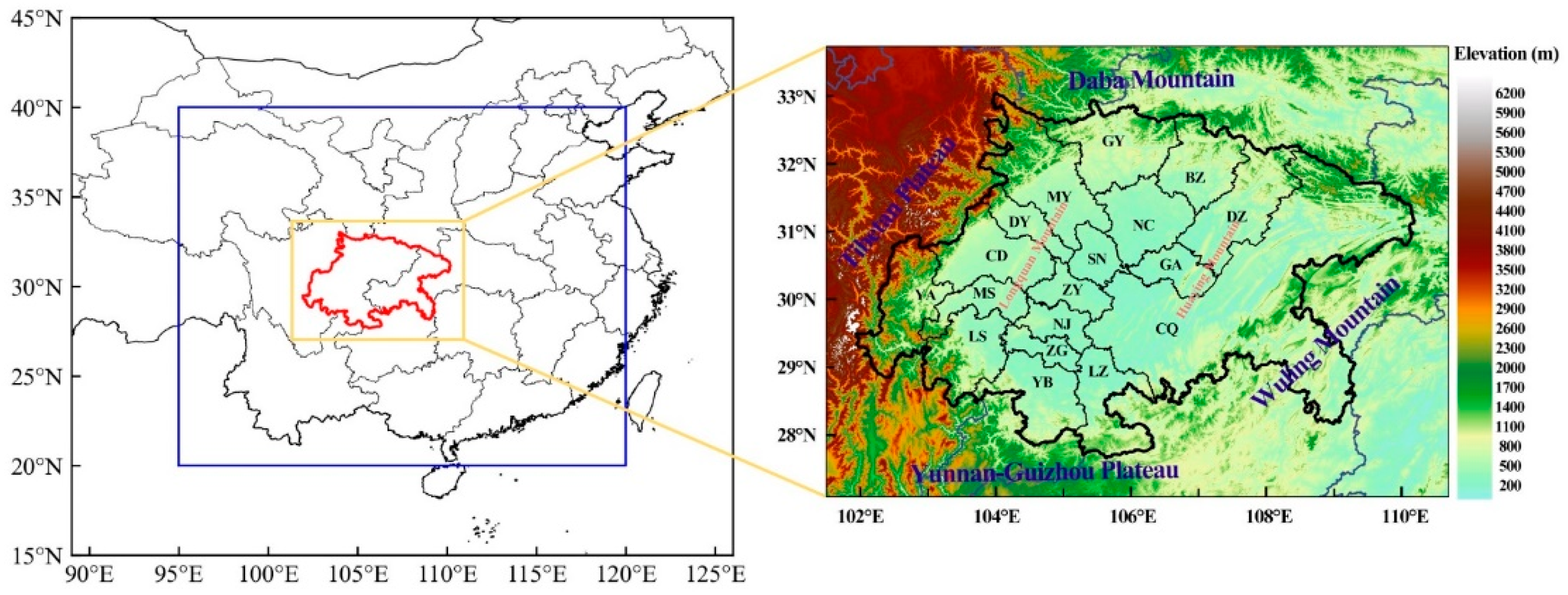
2.1. Study Area

This study covered the 18 prefecture-level cities in SCB, which were Chengdu (CD), Chongqing (CQ), Deyang (DY), Mianyang (MY), Meishan (MS), Leshan (LS), Ya’an (YA), Yibin (YB), Zigong (ZG), Luzhou (LZ), Neijiang (NJ), Ziyang (ZY), Suining (SN), Guangyuan (GY), Bazhong (BZ), Nanchong (NC), Dazhou (DZ) and Guang’an (GA). As shown in Figure 1, these cities were in the basin area confined by Tibetan Plateau to the west, Yunnan-Guizhou Plateau to the south, Wuling Mountain to the east and Daba Mountain to the North. The average altitude in the basin is about 400 m above sea level, while the altitudes of the plateaus and mountains are above 4000 m and 2000 m, respectively. The huge height drop creates lee-side calm area in the basin. Besides, the topography in the basin is also complicated, which could be divided into Chengdu Plain in the west, Hilly Area in the central basin and Ridge Valley area in the east by Longquan Mountain and Huaying Mountain.

2.2. PM2.5 Concentration Data and Spatial Characterization Method

The hourly PM2.5 concentration data of the state-controlled air-quality-monitoring sites in SCB from December 2015 to November 2019 were obtained from China National Environmental Monitoring Centre (https://air.cnemc.cn:18007/ (accessed on 1 December 2019)). The concentrations of all the sites in the same city were averaged to represent the urban PM2.5 concentration in this city. The annual PM2.5 concentration of a certain city was calculated by averaging the hourly data from January to November of the current year and December of the previous year. Correspondingly, winter was defined as January and February in the current year and December in the previous year in this study. Spring, summer and autumn were defined as March to May, June to August and September to November, respectively.
Two metrics were used to analyze the characteristics of spatial distribution of PM2.5 concentration in SCB. The first one was the coefficient of variation (CV) used to quantify the spatial disparity of PM2.5 concentration between 18 cities [12]. The CV was defined as CV = σ/Cm, in which σ and Cm were the standard deviation and the average of PM2.5 concentrations in 18 cities, respectively. During a certain period, the CV represented how uniformly the PM2.5 concentration distributed in the cities of SCB. Smaller CV indicated more obvious regional characteristics of PM2.5 pollution. The CV can characterize the variations in PM2.5 homogeneity but cannot reveal how these variations evolved. Hence, the relative spatial anomalies (RA) of average PM2.5 concentration for each city were used. RA for a certain city was calculated by RA = (Ci−Cm)/Cm, in which Ci and Cm were average PM2.5 concentration in this city and all cities, respectively. Therefore, larger RA meant relatively higher PM2.5 concentration in the relevant city compared to other cities. The inter-annual variation in CVs could provide the change in PM2.5 spatial disparity and the RAs could better show the spatial distribution of PM2.5 varying trend.

2.3. ERA5 Reanalysis Data and Objective Synoptic Classification

ERA5 dataset contains the fifth-generation atmospheric reanalysis data released by the European Center for Medium-Range Weather Forecasting (ECMWF). These data were obtained based on the 4D-Var data assimilation and model prediction of CY41R2 in the Integrated Forecasting System (IFS). Compared with its previous generation, namely ERA-interim, the horizontal and vertical resolutions of ERA5 were significantly improved, and the performance of ERA5 was better in the evaluation of tropospheric temperature, wind and humidity. Since the first release, ERA5 was widely used in research fields of atmospheric sciences, environmental issues [33,34,35,36], etc. ERA5 data at both upper-level isobaric surfaces and several single levels from December 1st 2015 to November 30th 2019 were collected. The data at 850 hPa, including potential height, relative humidity, temperature, vertical velocity and horizontal wind speed and direction, were used in this study. Besides, data at single levels, including surface pressure, 2 m temperature, 10 m horizontal wind speed and direction at ground level and PBLH, were used too. The data in full horizontal resolution (0.25° × 0.25°) and temporal resolution (1 h) were used.
The synoptic classification was conducted to explore the possible meteorological causes of the variation in PM2.5 spatial distribution. Synoptic classification could be carried out by subjective and objective methods, among which the subjective methods were mainly based on artificially defined a priori criteria and had great uncertainties [37]. On the contrary, objective methods were based on the maximization of similarity and variance; hence, these methods were appropriate for processing mass data without relying on a priori experiences [38]. The Cost733class package, a software jointly developed by Earth System Science and Environmental Management (ESSEM) and European Cooperation in Science and Technology (COST), focused on creating and evaluating weather and circulation-type classifications utilizing various different methods, including PCT (t-mode principal component analysis using oblique rotation), PTT (t-mode principal component analysis using orthogonal rotation), SOM (self-organizing maps) [39,40], etc. In this study, the PTT method was used to classify the synoptic patterns in SCB and its surrounding areas. The input data were the daily average geopotential heights at 850 hPa isobaric surface from ERA5 reanalysis data of ECMWF with a spatial resolution of 0.25° × 0.25°. The region implementing the synoptic classification was the area in 95° E~120° E and 20° N~40° N (Figure 1).

3. Results and Discussion

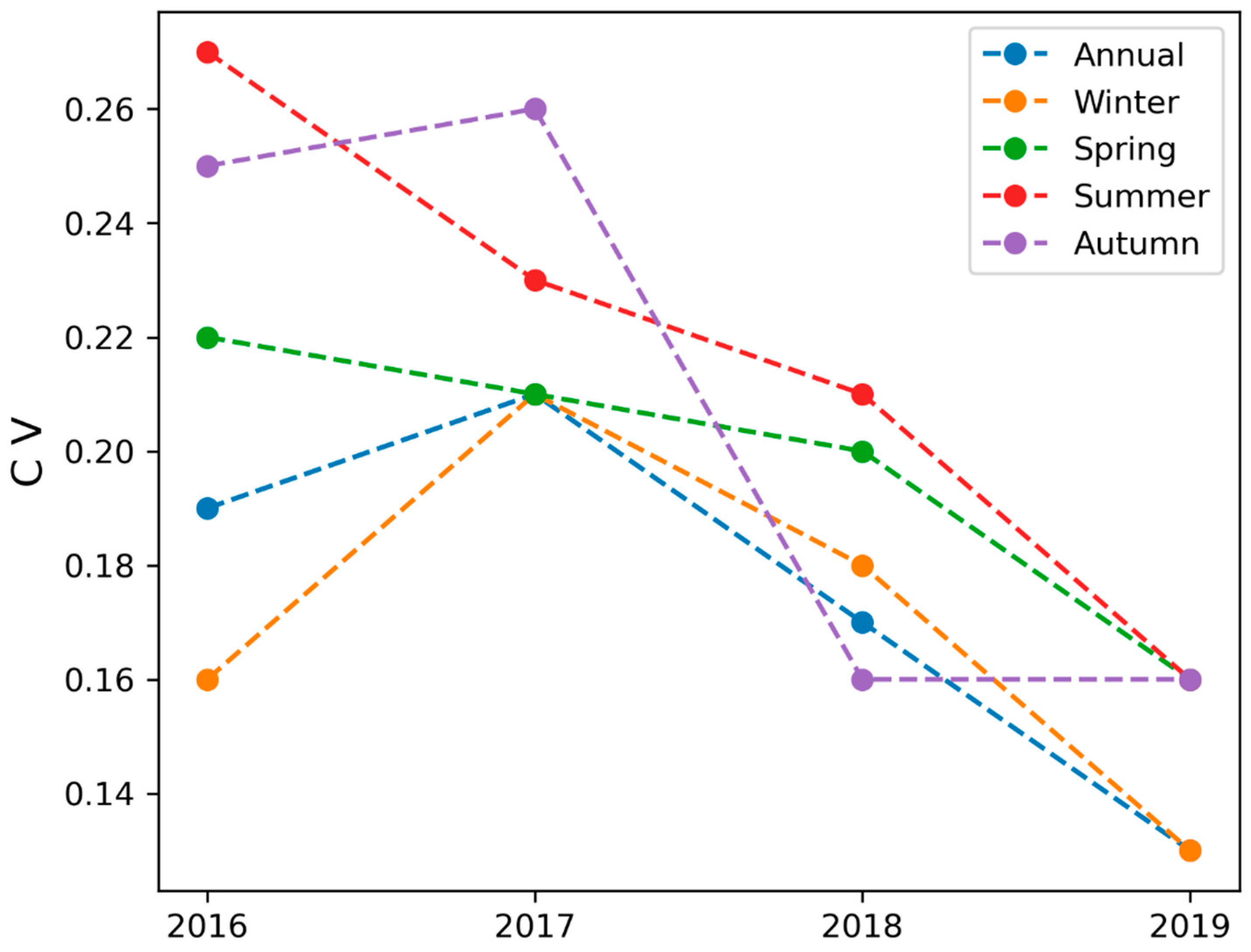
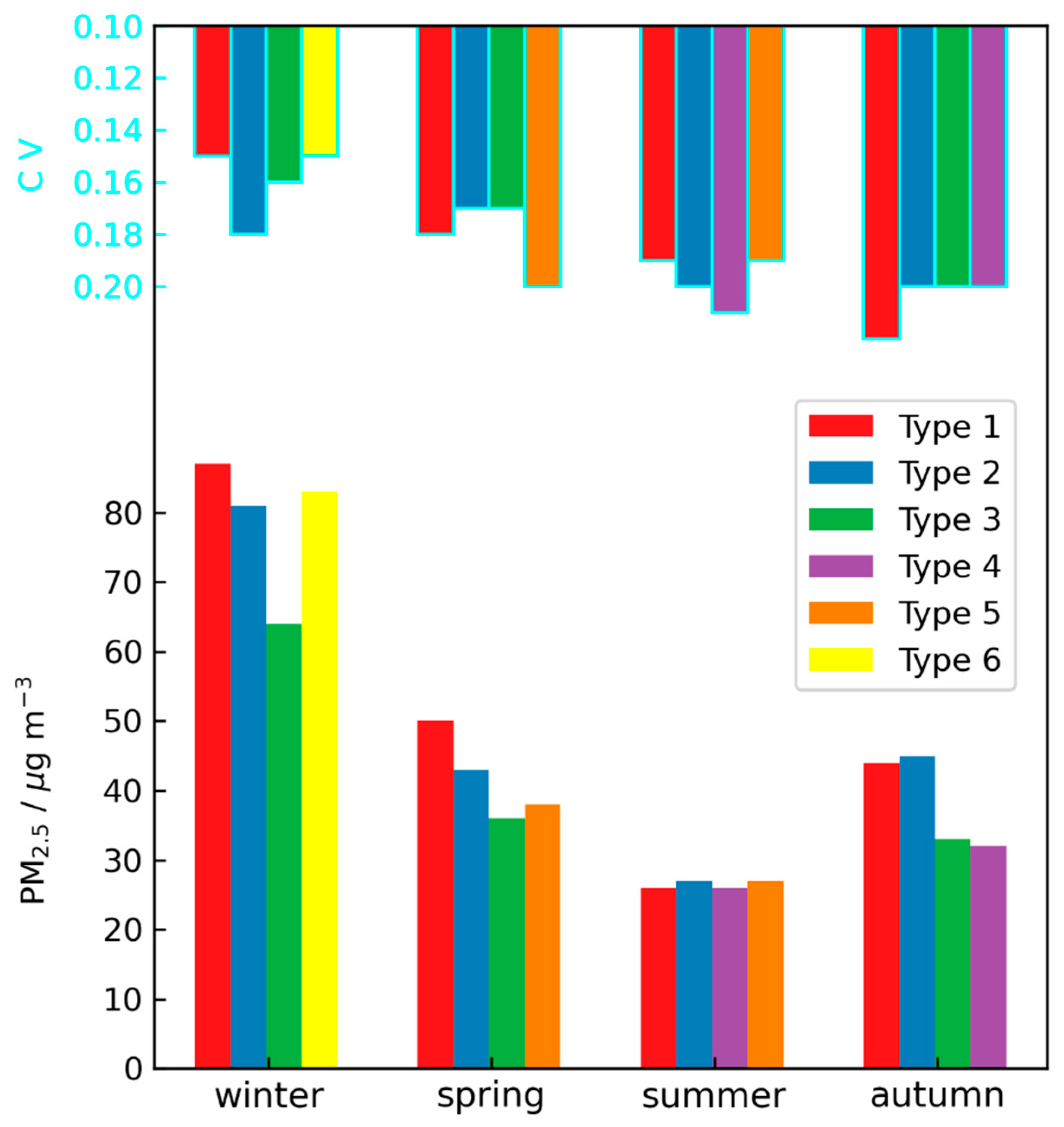
3.1. Variations in PM2.5 Spatial Disparity

The CVs of annual and seasonal PM2.5 concentrations are shown in Figure 2. The annual CVs showed a general decreasing trend from 2016 to 2019, except for slightly rebounding in 2017. This indicated that the differences in annual PM2.5 concentrations between 18 cities in SCB were narrowing. Similar variation trends were observed in other regions in China, such as North China Plain [41] and Northeastern China [42]. From the seasonal perspective, the CVs were the largest in summer among the four seasons, followed by spring and winter. This was partly due to the low average concentrations in summer (Table 1). The CVs in spring and summer decreased gradually from 2016 to 2019. The CV was 0.16 in the winter of 2016, but increased to 0.21 in 2017 and then gradually decreased to 0.13 in 2019. The spatial disparity varied more obviously in autumn than in other seasons. In the autumn of 2016 and 2017, the CVs were 0.25 and 0.26, respectively, and decreased to around 0.16 in 2018 and 2019. The smallest CV in 2018 was 38% lower than the largest value in 2017. In general, the spatial disparity of PM2.5 concentration in SCB decreased from 2016 to 2019, whether in terms of annual or seasonal average PM2.5 concentrations. In addition, it is worth noting that the CVs of the wintertime average PM2.5 concentration were close to those of annual averages. This revealed that the variation in PM2.5 distribution was dominated by wintertime PM2.5 distribution in SCB.
To explore the in-depth details about the variations in PM2.5 spatial disparity in SCB, the PM2.5 concentrations of 18 cities in SCB at annual and seasonal scales from 2016 to 2019 are shown in Figure 3. From the perspective of annual average PM2.5 concentrations, a rapid PM2.5 concentration decrease of 23 μg/m3, 15 μg/m3, 18 μg/m3 and 20 μg/m3 from 2016 to 2019 was observed in ZG, CD, LZ and MS, the most polluted cities in SCB. The PM2.5 concentrations of moderately polluted cities decreased more slowly. For example, the concentrations of CQ fell by 12 μg/m3 during these four years. However, the PM2.5 concentrations in GY and BZ, representing relatively lightly polluted cities, showed an increasing trend of 4 μg/m3 and 1 μg/m3, respectively. Hence, the decrease in PM2.5 concentrations in severely polluted cities and the maintaining (even increasing) of concentrations in moderately and lightly polluted cities together made the spatial disparity of PM2.5 concentration gradually decrease in SCB.
The inter-annual variations in wintertime PM2.5 concentrations presented a similar trend to the annual concentrations from 2017 to 2019, except before 2017. The PM2.5 concentrations in most cities increased from 2016 to 2017 and severely polluted cities showed a larger increase. The rising amount was 18 μg/m3, 29 μg/m3 and 19 μg/m3 in ZG, CD and MS, respectively. In the representative cities of moderately polluted cities, CQ, and lightly polluted cities, GY increased by 7 μg/m3 and decreased by 3 μg/m3, respectively. As a result, the range of concentrations in 18 cities became wider and wintertime CV increased significantly in 2017. From then to 2019, PM2.5 concentrations in ZG, CD and MS decreased significantly, by 40 μg/m3, 39 μg/m3 and 39 μg/m3, respectively. The concentration in CQ decreased only by 12 μg/m3 and the concentrations in GY and BZ rose by 5 μg/m3 and 2 μg/m3, respectively.
The inter-annual variations in PM2.5 concentrations in spring and summer were consistent with the annual trend. In autumn, the concentrations decreased in all cities at a similar rate from 2016 to 2017. However, much more obvious increasing trends were observed in moderately and lightly polluted cities from 2017 to 2018. The autumntime PM2.5 concentrations in BZ, GA, and GY increased by more than 10 μg/m3. Even the concentrations in CQ increased slightly as well. The reductions in autumntime concentrations in severely polluted cities, such as ZG, LZ and MS, were smaller than those in other seasons. This led to a significant reduction in spatial disparity in autumn of 2018 in SCB. From 2018 to 2019, the autumntime concentrations in most cities decreased at similar rates, hence, the spatial disparity remained stable, as shown in Figure 2.

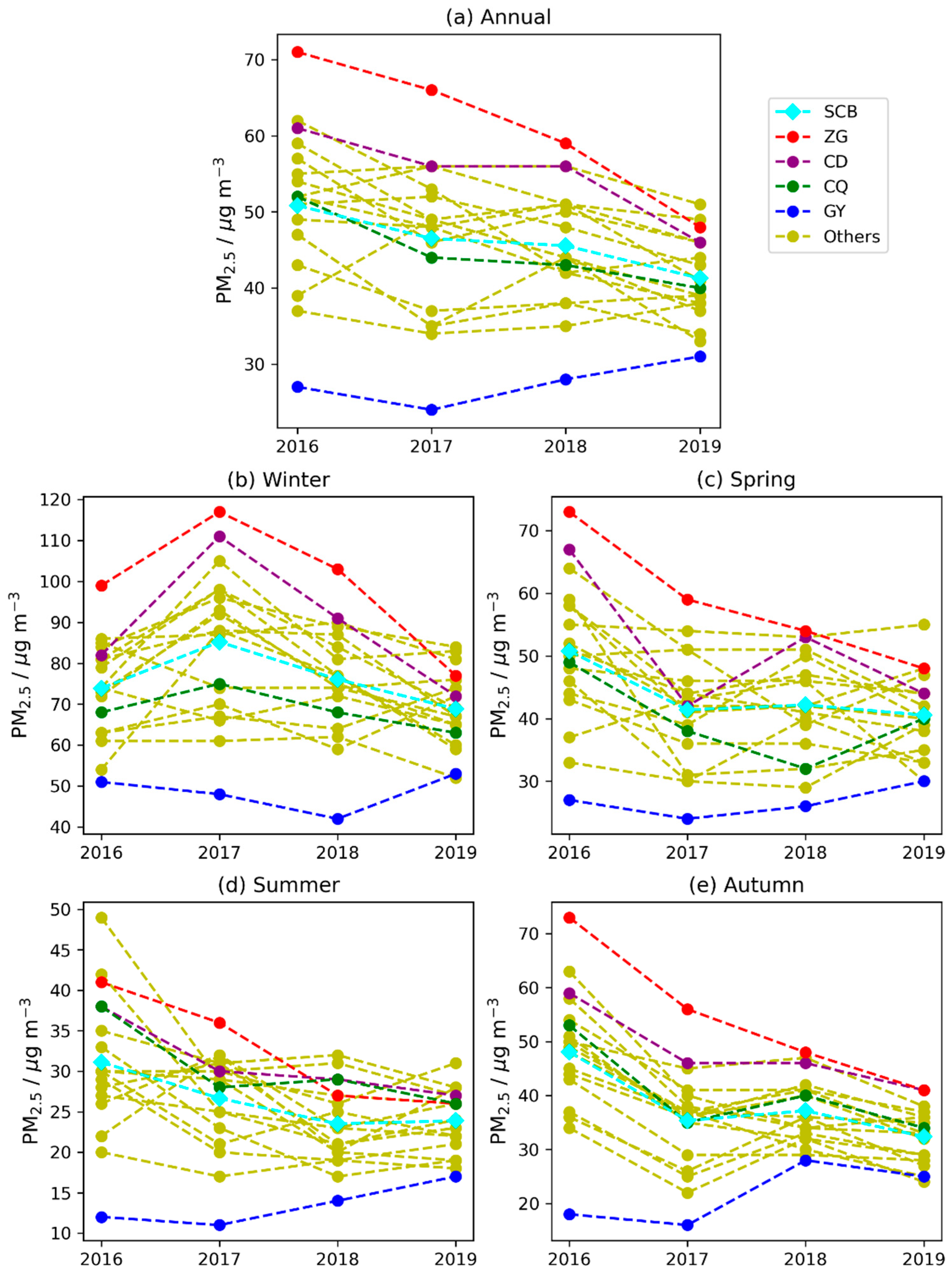
3.2. Variations in PM2.5 Spatial Distribution

The spatial distribution of RAs in annual average concentrations can be found in Figure 4. In 2016, the PM2.5 concentrations of most cities in the western (CD, MS and LS) and south parts (ZG, YB and LZ) of SCB were highest, inferred from the distribution of positive RAs in these areas. The RAs of cities in the northeast part of SCB were slightly positive (DZ and NC) or negative (GY, BZ, GA), revealing relatively lower concentrations in this area. In 2017, in total, 10 cities held positive RAs, among which 9 cities were located in the western and southern parts of SCB, except DZ in the northeast part, including CD, DY, MY, MS, YA, LS, ZG, YB and LZ. Moreover, the RAs of these cities were higher than those in 2016, resulting in larger spatial disparity in annual average concentrations in 2017, as shown in Figure 2. In 2018 and 2019, cities with positive RAs were distributed in the south (ZG, YB and LS), the northwest (CD, DY and MY) and the northeast (DZ and NC) parts of SCB. Another feature was that the RA in MS (LZ) decreased (increased) significantly from 2018 to 2019. The variations in RA distribution further suggested that spatial disparity of annual average PM2.5 concentrations was declining in SCB because the maximum RA decreased from 2016 to 2019 and the variations in RAs showed obvious regional characteristics, decreasing in the western and southern basin and increasing in the northern basin.
Generally, the variation features of RAs in seasonal average PM2.5 concentrations were coincident with those of the annual averages. In winter, the RAs in the western and southern parts of SCB were much higher than those in other parts and kept decreasing from 2016 to 2019. The lowest RAs were found in the northern part of SCB, such as GY and BZ and the RAs in this area increased significantly from 2016 to 2019, especially in 2019. In spring and autumn, the RAs in GY and BZ increased more significantly than in winter, while the RAs in the western and southern parts of SCB were decreasing. In summer, the RA in CQ was higher than that in other seasons, and the RAs in the northern part of SCB maintained the values in other seasons.
In summary, the spatial disparity of PM2.5 concentrations of 18 cities in SCB narrowed and the variations in concentrations showed prominent regional characteristics, namely decreasing in the western and southern basin, maintaining in the central and eastern basin, and slightly increasing in the northern basin. These regional characteristics suggested that the meteorological conditions might be important causes, especially the increase in concentrations in the northern basin, despite strict emission control measures. Therefore, in the next section, the synoptic patterns were identified and their impacts on the distribution of atmospheric diffusion conditions were analyzed, aiming to explain the regional maintaining or increasing trends of PM2.5 concentration in the northeastern basin.

3.3. Synoptic Patterns and Their Impacts on PM2.5 Spatial Distribution

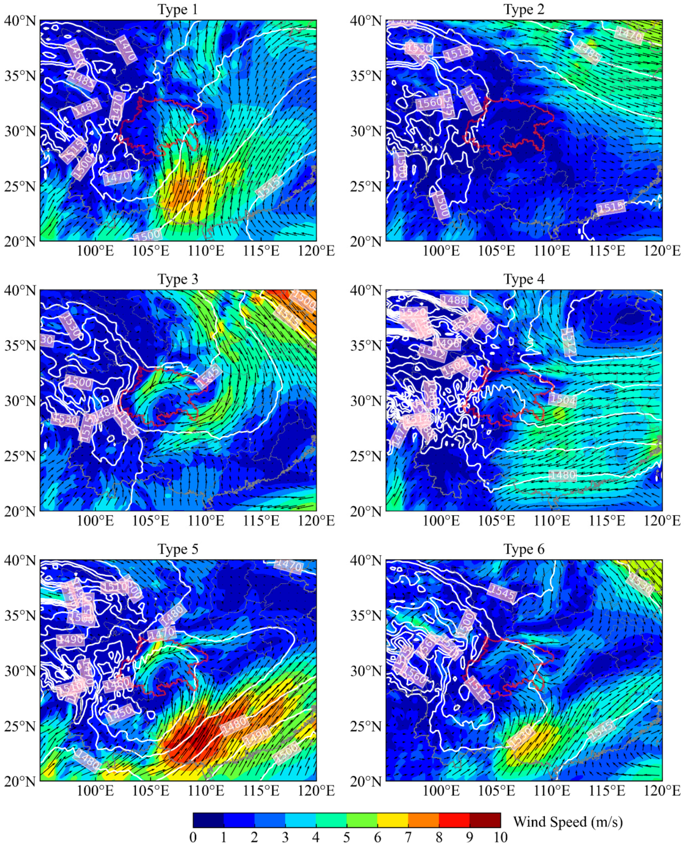
3.3.1. Identified Synoptic Patterns

By implementing the PTT classification method, the synoptic patterns in SCB and the surrounding area were classified into nine types in total, according to the daily average geopotential heights at 850 hPa, from 1 December 2015 to 30 November 2019. Among these patterns, the last three types occurred in less than 10 days and the first six types occurred in more than 98.8% of the days accumulatively. Hence, only the first six patterns were analyzed in this study, and their occurring days are shown in Table 2.
The first synoptic pattern occurred in 432 days, out of 1443 days in total, which was much more than other types. The occurring days of Types 2–6 were 286, 252, 242, 172 and 59 days, respectively. Seasonally, Type 1 and Type 2 almost evenly occurred throughout the four seasons. The occurrence frequencies of Type 3 were highest in winter, followed by autumn and spring, but only occurred on 3 days in summer. On the contrary, the occurrence frequencies of Type 4 were relatively higher in summer and autumn, and close to zero in winter and autumn. Type 5 occurred more frequently in spring and summer than the other two seasons, while Type 6 almost occurred only in winter. Therefore, we mainly discussed Type 1, Type 2, Type 3 and Type 6 in winter, Type 1, Type 2, Type 3 and Type 5 in spring, Type 1, Type 2, Type 4 and Type 5 in summer, and Type 1, Type 2, Type 3 and Type 4 in autumn.
The spatial distribution characteristics of 850 hPa potential heights for six synoptic patterns are shown in Figure 5. In Type 1, the SCB was controlled by a weak low-pressure system, noted as weak low-pressure type. When Type 2 occurred, the SCB was under the control of a weak high-pressure system and uniform pressure fields (weak high-uniform-pressure type). In Type 3, there was a strong high-pressure center to the north of SCB, noted as northern high-pressure type. Type 4 could be summarized as eastern weak high-pressure type for the existence of a weak high-pressure center to the east of SCB. Similarly, Type 5 could be named as southwestern weak low-pressure type for the existence of a weak low-pressure center to the southwest. Type 6 was also characterized with the control of a weak low-pressure system, just as Type 1, but collocating a high-pressure system to the north of SCB, noted as weak low-pressure with northern high-pressure type.
Figure 5 presents the wind fields at 850 hPa for the six synoptic patterns in SCB. In Type 1, the regions to the east of SCB prevailed southerly winds. Air masses originated in southern China, such as Guangxi and Guangdong provinces, and entered the SCB through the southeastern edge of the basin (the south part of CQ). This air flows towards the north through the central and eastern basin, and turns west in the western basin. Affected by the topography, the wind speeds in the western basin were relatively low. In Type 2, the uniform pressure fields led to extremely calm winds in the basin. The northeast part of the basin was controlled by the westerly or northwesterly air flows. Type 3 presented prevailing strong northerly winds in the areas to the east of SCB. These strong northerly winds entered SCB through the high mountains in the north and caused a relatively strong wind zone in the northern basin and western basin. The cyclonic circulation converged in the southeastern basin and led to a calm wind zone there. In Type 4, easterly winds invaded SCB through the eastern part of the basin area and turned south in the western part of the basin. This circulation pattern made the wind velocity in the southern part of the basin extremely low. In Type 5, although southerly winds prevailed in the area to the southeast of SCB, the air masses from the south could not cross over the mountains in the southeastern edge of the basin. Hence, the basin was mainly affected by the northerly air flows and created similar circulations as Type 3. The circulation features in Type 6 were similar to those in Type 5 but the wind speeds were relatively lower.

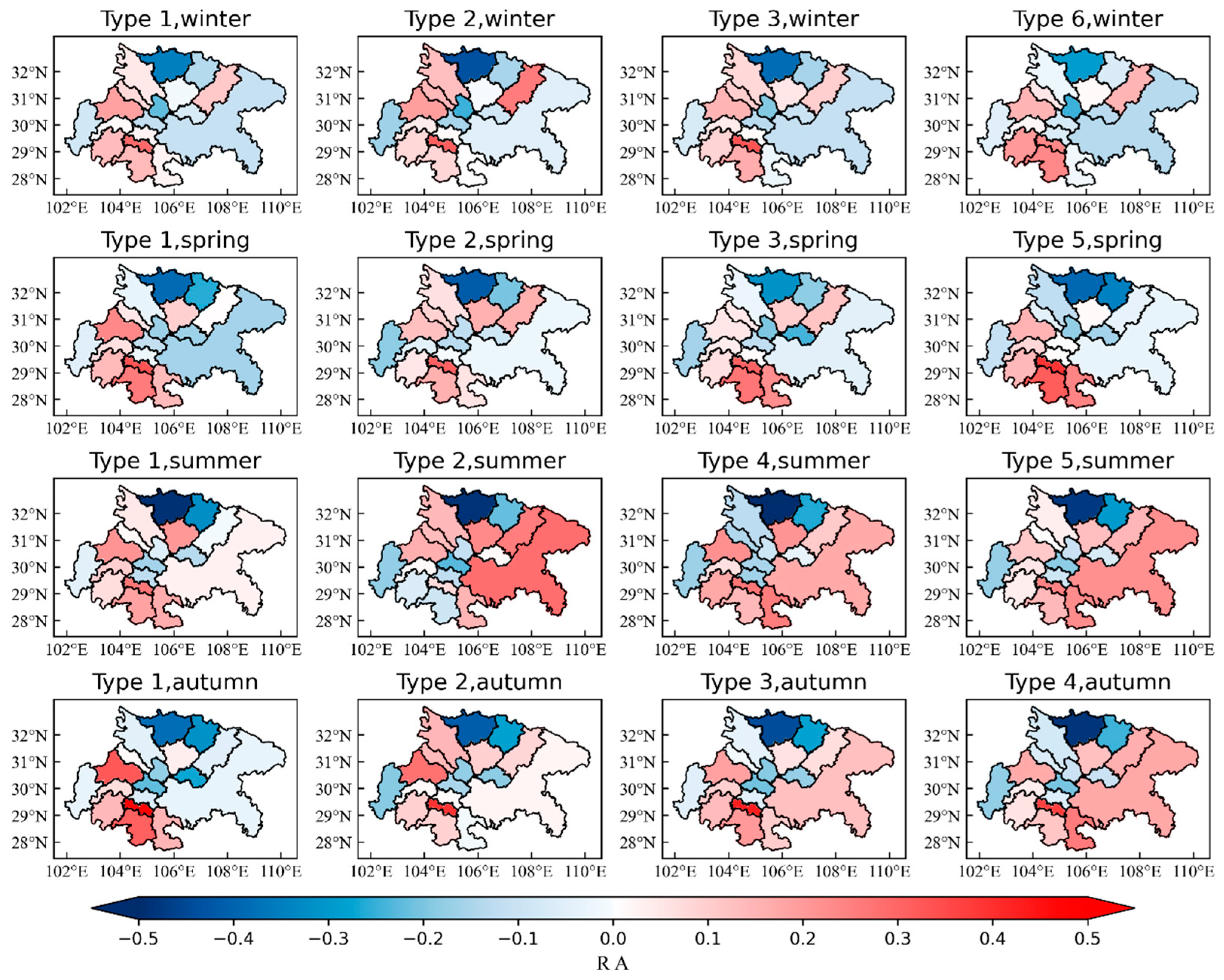
3.3.2. The Impacts of Synoptic Patterns on PM2.5 Spatial Distribution

Figure 6 shows the average PM2.5 concentrations and their CVs in SCB for six synoptic patterns. The PM2.5 concentrations of different synoptic patterns were almost the same in summer, around 26 μg/m3. In other three seasons, the concentrations of Type 1 and Type 2 were relatively higher than those of Type 3. In winter, PM2.5 concentrations exceeded 80 μg/m3 in Type 1 and Type 2 and only 64 μg/m3 in Type 3. The PM2.5 concentrations of Type 1, Type 2 and Type 3 were 50μg/m3, 43μg/m3 and 36μg/m3 in spring, and 44 μg/m3, 45 μg/m3 and 33 μg/m3 in autumn, respectively. In addition, the concentration of Type 6 also exceeded 80 μg/m3 in winter and the concentrations of Type 5 in spring and Type 4 in autumn were relatively low, about 38 μg/m3 and 32 μg/m3, respectively. Therefore, Type 1, Type 2 and Type 6 were more conducive to the formation of PM2.5 pollution, and the air quality was relatively better in Type 3, Type 4 and Type 5. From the perspective of the spatial disparity, the largest CVs were 0.18 (in Type 2), 0.20 (in Type 5), 0.21 (in Type 4) and 0.22 (in Type 1) in winter, spring, summer and autumn, respectively. This indicated that the CVs were not related to concentrations.
The spatial distribution of RAs in four seasons for different synoptic patterns is shown in Figure 7. In winter, the distribution of RAs for Type 1, Type 3 and Type 6 was consistent to the average feature, as shown in Figure 4. However, in Type 2, the RAs in the northwestern basin (CD, DY and MY) were higher than those in the southern basin and the RA in GY showed a relatively low value compared with the other types. The ranges in wintertime RAs were relatively large in Type 2 and small in Type 6. In spring, Type 1 and Type 5 presented more prominent regional characteristics, with higher (lower) RAs in the western and southern (northern) basin. Comparatively, Type 2 and Type 3 showed relatively higher RAs in the northern basin and lower RAs in the western and southern basin. The largest and smallest variation ranges of RAs occurred in Type 5 and Type 2, respectively. In summer, Type 1 showed a similar RA distribution to Type 1 in spring. Type 2 presented a distinct distribution feature with lower RAs in the southern basin and higher RAs in the eastern and northeastern basin. The RA was only 0.08 in ZG and actually negative in YB and LS. The highest RAs were distributed in CQ, DZ and NC. Type 4 and Type 5 showed similar RA distribution characteristics but with higher (lower) RAs in the southern (northern) basin compared with Type 2. In autumn, the RA distribution feature of Type 1 was similar to that of Type 5 in spring, and the distribution features of Type 3 and Type 4 were similar to that of Type 5 in summer. Type 2 showed a different distribution. The RA of ZG was the largest, exceeding 0.40, but the RAs of other southern cities were lower than 0.10. RAs in the western basin were larger than the remaining regions, but the difference was small compared with other types in autumn.

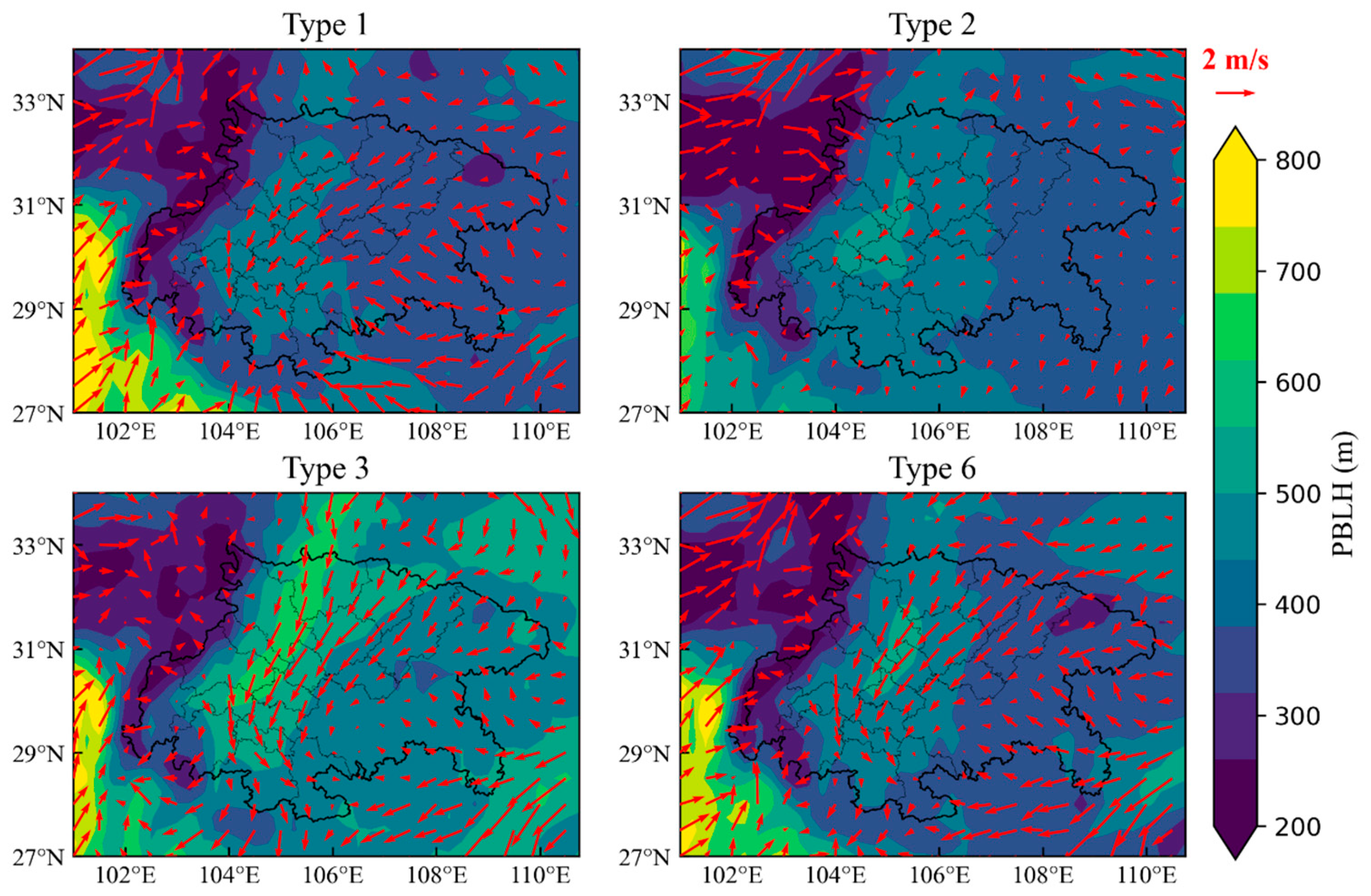
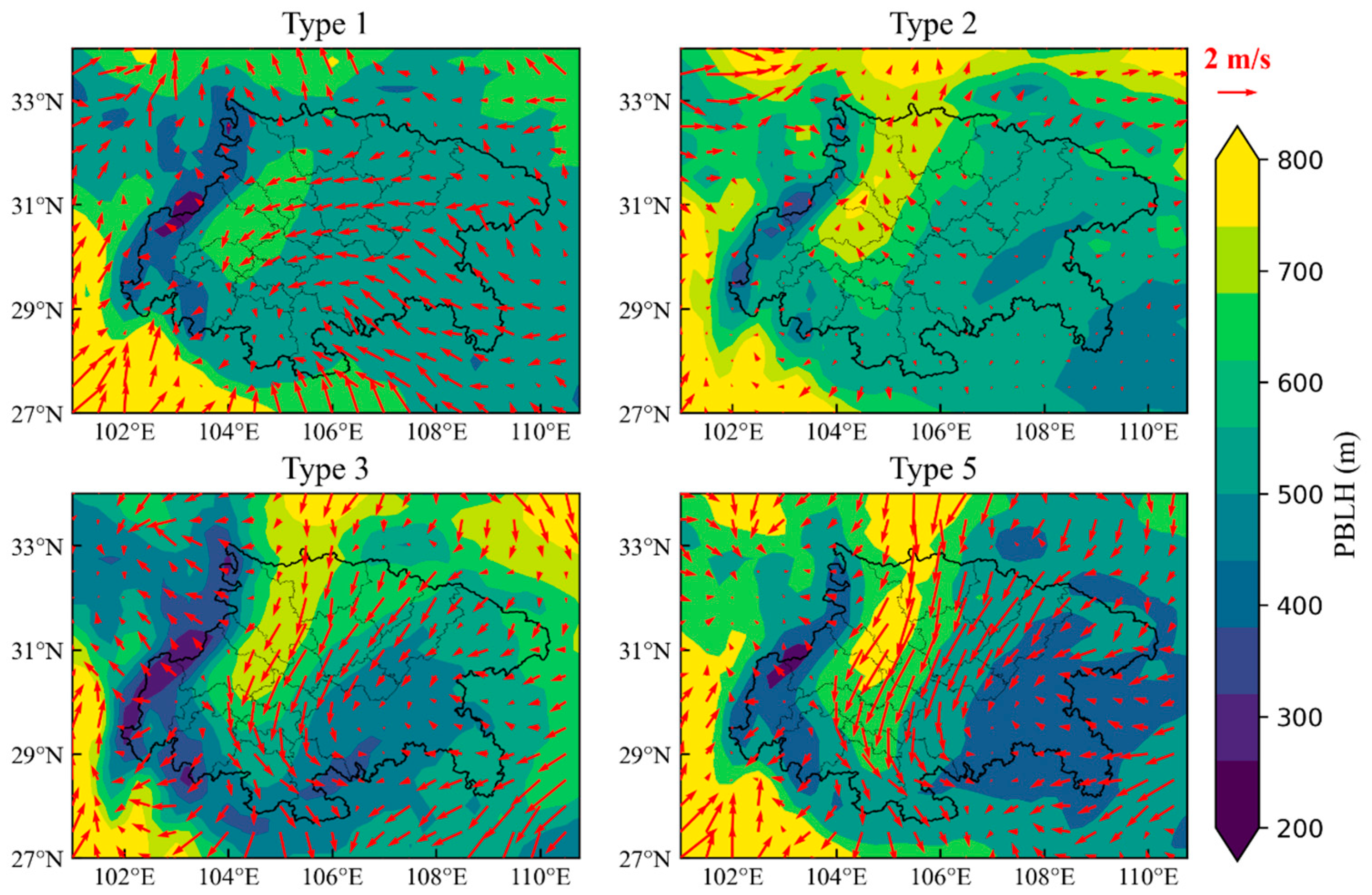
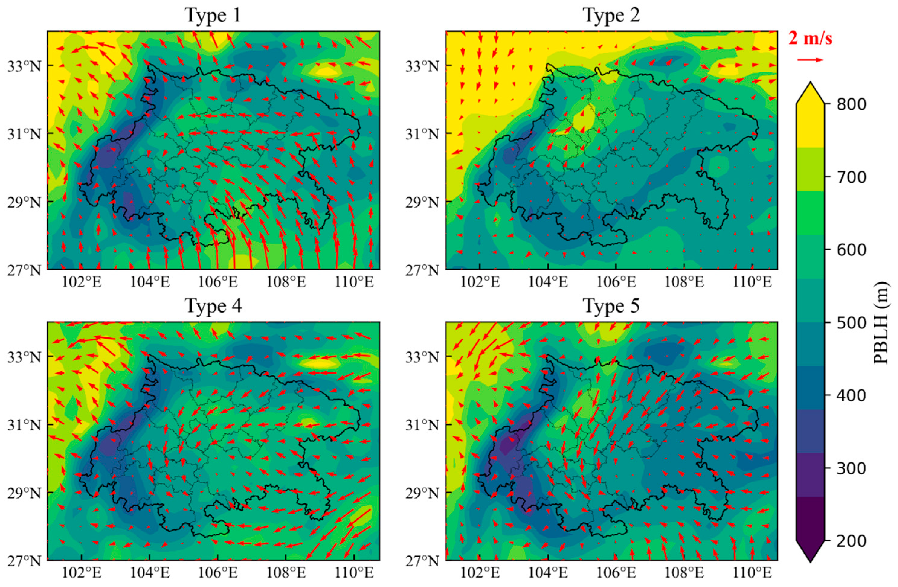
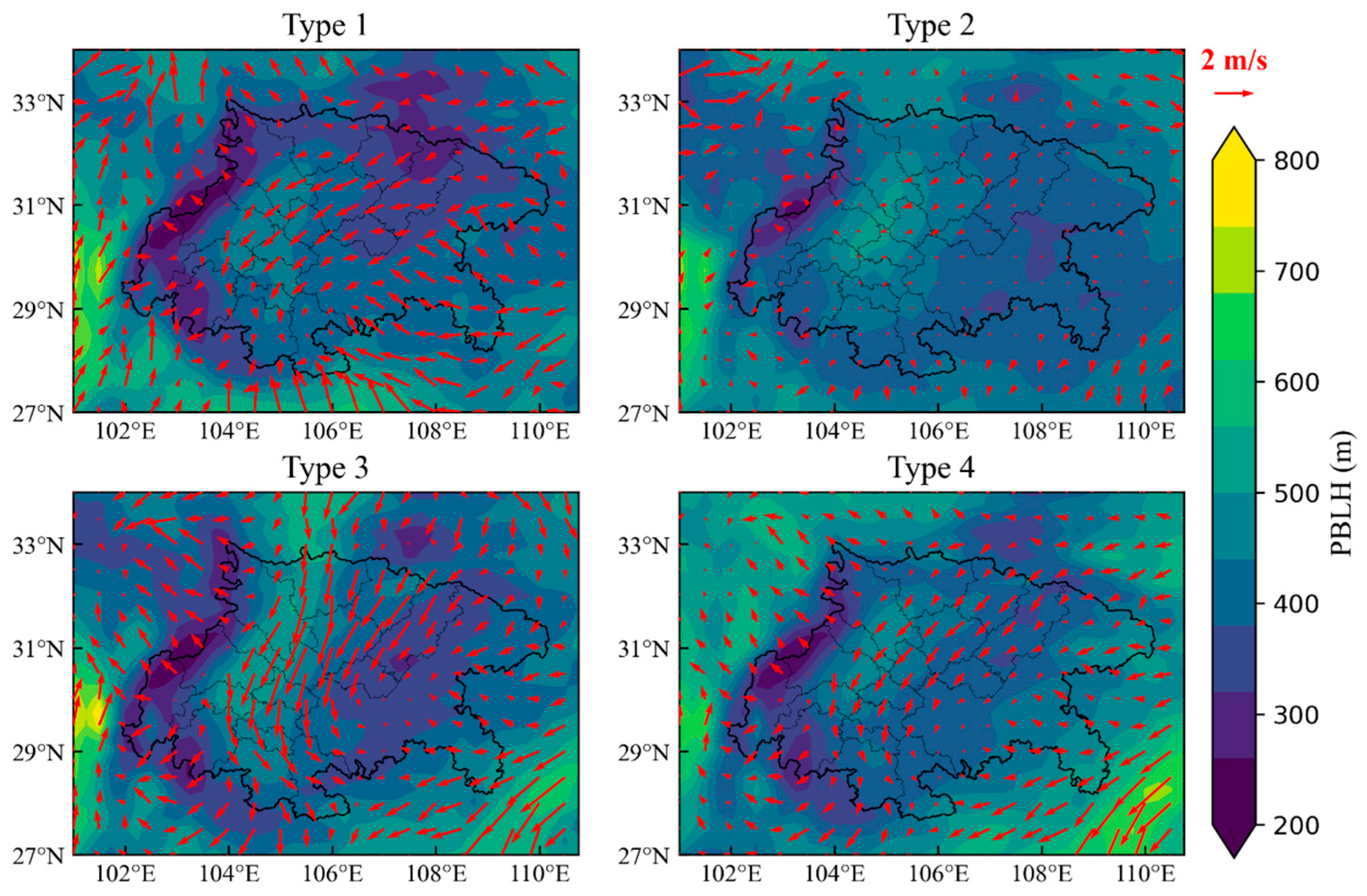
3.3.3. The Mechanisms of the Impacts of Synoptic Patterns on PM2.5 Spatial Distribution

PBLH and horizontal wind were key meteorological factors to measure the vertical and horizontal diffusion ability of air pollutants [43]. Hence, the PBLH and 10 m wind fields over SCB in four seasons were extracted from ERA5 reanalysis data and these fields for different synoptic patterns are presented in Figure 8, Figure 9, Figure 10 and Figure 11. In winter (Figure 8), the main meteorological feature was the relatively high PBLH area covering the central basin, including the eastern parts of MY, DY, CD and MS, the western parts of ZY and SN, and the southern part of GY. The covering regions and PBLH values, collocating with horizontal wind fields and emissions, determined the distribution of PM2.5. Type 3 presented the highest PBLH and strongest winds, and correspondingly, the average PM2.5 concentration was the lowest. In Type 2, the low PBLH and calm winds were conducive to the accumulation of pollutants. Hence, the distribution of emissions was the dominant factor influencing PM2.5 distribution, which made the RAs vary in relatively larger ranges in Type 2. In Type 1 and Type 6, the regions with massive emissions, such as the western and southern basin, were controlled by the high-PBLH area and relatively strong winds. This made the diffusion condition in higher emission areas better than other areas. As a result, the spatial disparity of PM2.5 concentrations in Type 1 and Type 6 was lower.
In spring, the PBLH in the basin was significantly higher than those in winter. Hence, the wind-induced transportation of air pollutants might be the main factor determining PM2.5 distribution. In Type 5 and Type 3, northerly winds invaded the basin from GY, BZ and DZ, blew straight southwards and converged in the southern and southeastern basin. This flow field could transport air pollutants to the south and aggravate the pollution in the southern basin. Meanwhile, the downwind regions confronted low-PBLH conditions. Consequently, these factors led to the relatively high RAs in the southern basin. In Type 2, the wind speeds were the lowest and pollutant transport was limited. Additionally, the relatively high PBLH in the western and southern basin promoted the diffusion of pollutants in massive emission areas. Therefore, the difference in PM2.5 concentrations in SCB was relatively low. The winds in Type 1 blew from east to west and turned south near the western edge of the basin, which caused higher RAs in the western and southern basin.
In summer, the wind fields were also the dominant factors influencing PM2.5 distribution because of the relatively uniformly distributed PBLH. Similar wind fields were observed in Type 1 compared to those of Type 1 in spring, and resulted in higher RAs in the western and southern basin. The weak southerly winds prevailed in Type 2, with relatively larger velocities in the northeastern basin (CD, DY and MY) and the low PBLH controlled the eastern and southern basin. These made the higher RAs distribute in the northeastern basin (CD, DY, MY) and eastern basin (DZ and CQ). Type 4 and Type 5 presented similar cyclonic circulation in SCB, which led to calm winds in the southern and eastern basin and resulted in higher RAs in these regions. Furthermore, the air masses from north entered SCB through western pathways and the northerly winds in the western basin were stronger in Type 5. Hence, the RAs in the western basin were lower in Type 5 than those in Type 4.
The wind fields were the dominant factors in autumn due to the relatively low and uniformly distributed PBLH. In Type 1, easterly winds invaded SCB from the northeast basin corner and caused prevailing northwesterly winds in the basin. The transport of air pollutants caused the relatively higher RAs in the western and southern basin. Extreme stagnation conditions occurred in Type 2 and made the high RAs distribute in massive emission areas. Type 3 and Type 4 presented similar northerly invasion air flows and caused cyclonic circulation, converging in the eastern basin. The pollutant transport and calm-wind-induced stagnation led the higher RAs in the southern basin and eastern basin, respectively. The relatively stronger winds in Type 4 more thoroughly transported the pollutants to the downwind areas, so lower RAs were observed in LS and YB compared with those in Type 3.

3.3.4. The Synoptic Causes of PM2.5 Distribution Variations

From previous analysis, we could conclude that the spatial disparity of PM2.5 concentration was gradually decreasing in SCB and presented prominent regional characteristics of declining in the western and southern basin, maintaining in other regions and even increasing in the northern and northeastern basin. In this section, possible synoptic causes of this phenomenon are analyzed. Because the PM2.5 concentrations in summer were relatively low (Figure 6) and the occurrence frequencies of identified summertime synoptic patterns varied slightly, except in Type 1, as shown in Table 2, the synoptic causes in summer were not analyzed.
In winter, the two synoptic patterns with the two largest CVs, Type 2 and Type 3, occurred in declining frequencies. As shown in Table 2, the occurrence days of Type 2 and Type 3 decreased from 17 days and 42 days to 9 days and 20 days, respectively, during 2016–2019. On the contrary, the synoptic patterns with the smallest CV (Type 6) occurred more frequently, from 5 days to 26 days. Along with the metric of CV, the average PM2.5 concentration in the northern basin (GY, BZ, NC and DZ) was largest in Type 6, reaching 79 μg/m3, and smallest in Type 3, only 58 μg/m3. Therefore, the growth in Type 6 and the reduction in Type 3 and Type 2 could be the reasons for the decrease in spatial disparity in SCB and the increase in RAs in the northern basin in winter.
In spring, the synoptic patterns with higher CVs, Type 5 and Type 1, were increasing and the synoptic patterns with lower CVs, Type 3 and Type 2, were decreasing. Type 1 occurred in 40 days in 2016 and 26 days in 2019. The occurrence days slightly declined from 18 days to 15 days, while Type 2 and Type 3 grew from 17 days and 9 days to 28 days and 16 days, respectively. Specifically, the RAs in the northern basin (NC, DZ and BZ) for Type 2 and Type 3 were relatively larger than those for Type 1 and Type 5. Hence, the reduction in Type 1 and Type 5 and the growth in Type 2 and Type 3 could reduce the spatial disparity of PM2.5 in SCB, and explain the increasing RAs in the northern basin in spring.
In autumn, the occurrence frequencies of all synoptic patterns in 2019 remained almost the same as those in 2016. This was consistent with the fact that the distribution in RAs varied slightly, as shown in Figure 4. In detail, the difference in RAs between the western and northern basin began narrowing from 2017. Correspondingly, Type 2, in which the RAs in the northwestern basin (CD, DY and MY) were higher than other cities, occurred in more days, and Type 3 and Type 4, in which RAs in the northwestern basin were lower, occurred in fewer days.

4. Conclusions

In this study, the spatial disparity of PM2.5 concentrations in SCB and its variation characteristics were explored, and the possible synoptic causes of these variations were analyzed. It was found that the spatial disparity of PM2.5 concentrations in SCB narrowed from 2016 to 2019. This tendency towards conformity of PM2.5 distribution was the result of a decreasing trend in cities with high concentrations, maintaining trend in cities with moderate concentrations and increasing trend in cities with low concentrations. Spatially, the main feature was that PM2.5 pollution was improved in the western and southern basin and deteriorated in the northern basin, especially in GY and BZ.
The regional characteristics of PM2.5 distribution variations could be partly interpreted by the occurrence frequencies of typical synoptic patterns, including weak low-pressure type (Type 1), weak high-pressure system and uniform pressure fields (Type 2), northern high-pressure type (Type 3), eastern weak high-pressure type (Type 4), southwest weak low-pressure type (Type 5), and weak low-pressure with northern high-pressure type (Type 6). Type 1, Type 2 and Type 6 were related to more polluted weather and Type 2, Type 3 and Type 5 were linked to cleaner days. The synoptic patterns influenced the PM2.5 distribution by modulating the diffusion conditions through PBLH and wind fields. The reduction in Type 2 and Type 3 (Type 1 and Type 5) and the growth of Type 6 (Type 2) led to a decrease in spatial disparity in winter (spring). Moreover, diffusion conditions (PBLH and wind) were the most important meteorological conditions affecting PM2.5 concentration and spatial distribution in SCB.
It was worth noting that the emission control measures were key factors that led to an improvement in air quality, although the impacts of synoptic patterns were manifested in this study. Specifically, the fact that PM2.5 concentration declined at a faster rate in more polluted cities might be the result of easier and more effective emission reduction in these areas. However, the regional maintaining, even rebounding, of PM2.5 concentration in the northern and northeastern basin could not be easily explained by emission variation alone, because a continuous reduction in emissions was expected, considering the implemented policies. Hence, the results of this study provide rational interpretation to this extraordinary trend on one hand. On the other hand, the fluctuation in PM2.5 concentration caused by synoptic circulation implied that the emissions in these areas might be close to the atmospheric capacity already. Implementing more precise and effective emission control measures is urgent to continuously improve the air quality.

Author Contributions

Conceptualization, G.S.; methodology, X.X.; investigation, X.X. and X.W.; writing—original draft preparation, X.X.; writing—review and editing, G.S. and F.Y.; supervision, F.Y. All authors have read and agreed to the published version of the manuscript.

Funding

This research was funded by the National Key R&D Program of China, grant number 2018YFC0214002 and 2018YFC0214001; the Key S&T Program of Sichuan Province, grant number 2018SZDZX0023; the National Natural Science Foundation of China, grant number 22076129; the Fundamental Research Funds for the Central Universities, grant number 41875162 and 22076129; the Young Talent Team Science and Technology Innovation Project of Sichuan Province, grant number 2020JDTD0005.

Institutional Review Board Statement

Not applicable.

Informed Consent Statement

Not applicable.

Conflicts of Interest

The authors declare no conflict of interest.

References

  1. Green, M.C.; Chen, L.W.A.; DuBois, D.W.; Molenar, J.V. Fine particulate matter and visibility in the Lake Tahoe Basin: Chemical characterization, trends, and source apportionment. J. Air Waste Manag. Assoc. 2012, 62, 953–965. [Google Scholar] [CrossRef] [Green Version]
  2. Silva, R.A.; Adelman, Z.; Fry, M.M.; West, J.J. The Impact of Individual Anthropogenic Emissions Sectors on the Global Burden of Human Mortality due to Ambient Air Pollution. Environ. Health Perspect. 2016, 124, 1776–1784. [Google Scholar] [CrossRef] [Green Version]
  3. Wang, Y.G.; Ying, Q.; Hu, J.L.; Zhang, H.L. Spatial and temporal variations of six criteria air pollutants in 31 provincial capital cities in China during 2013–2014. Environ. Int. 2014, 73, 413–422. [Google Scholar] [CrossRef] [PubMed]
  4. Guo, Y.M.; Zeng, H.M.; Zheng, R.S.; Li, S.S.; Barnett, A.G.; Zhang, S.W.; Zou, X.N.; Huxley, R.; Chen, W.Q.; Williams, G. The association between lung cancer incidence and ambient air pollution in China: A spatiotemporal analysis. Environ. Res. 2016, 144, 60–65. [Google Scholar] [CrossRef] [PubMed]
  5. Cohen, A.J.; Brauer, M.; Burnett, R.; Anderson, H.R.; Frostad, J.; Estep, K.; Balakrishnan, K.; Brunekreef, B.; Dandona, L.; Dandona, R.; et al. Estimates and 25-year trends of the global burden of disease attributable to ambient air pollution: An analysis of data from the Global Burden of Diseases Study 2015. Lancet 2017, 389, 1907–1918. [Google Scholar] [CrossRef] [Green Version]
  6. Albrecht, B.A. Aerosols, Cloud Microphysics, and Fractional Cloudiness. Science 1989, 245, 1227–1230. [Google Scholar] [CrossRef]
  7. Guo, J.P.; Liu, H.; Li, Z.Q.; Rosenfeld, D.; Jiang, M.J.; Xu, W.X.; Jiang, J.H.; He, J.; Chen, D.D.; Min, M.; et al. Aerosol-induced changes in the vertical structure of precipitation: A perspective of TRMM precipitation radar. Atmos. Chem. Phys. 2018, 18, 13329–13343. [Google Scholar] [CrossRef] [Green Version]
  8. Yang, X.; Zhao, C.F.; Guo, J.P.; Wang, Y. Intensification of aerosol pollution associated with its feedback with surface solar radiation and winds in Beijing. J. Geophys. Res.-Atmos. 2016, 121, 4093–4099. [Google Scholar] [CrossRef]
  9. Mu, M.; Zhang, R.H. Addressing the issue of fog and haze: A promising perspective from meteorological science and technology. Sci. China-Earth Sci. 2014, 57, 1–2. [Google Scholar] [CrossRef] [Green Version]
  10. Wang, H.J.; Chen, H.P. Understanding the recent trend of haze pollution in eastern China: Roles of climate change. Atmos. Chem. Phys. 2016, 16, 4205–4211. [Google Scholar] [CrossRef] [Green Version]
  11. Ning, G.C.; Wang, S.G.; Ma, M.J.; Ni, C.J.; Shang, Z.W.; Wang, J.X.; Li, J.X. Characteristics of air pollution in different zones of Sichuan Basin, China. Sci. Total Environ. 2018, 612, 975–984. [Google Scholar] [CrossRef] [PubMed]
  12. He, J.J.; Gong, S.L.; Yu, Y.; Yu, L.J.; Wu, L.; Mao, H.J.; Song, C.B.; Zhao, S.P.; Liu, H.L.; Li, X.Y.; et al. Air pollution characteristics and their relation to meteorological conditions during 2014–2015 in major Chinese cities. Environ. Pollut. 2017, 223, 484–496. [Google Scholar] [CrossRef] [PubMed]
  13. Su, F.C.; Xu, Q.X.; Wang, K.; Yin, S.S.; Wang, S.B.; Zhang, R.Q.; Tang, X.Y.; Ying, Q. On the effectiveness of short-term intensive emission controls on ozone and particulate matter in a heavily polluted megacity in central China. Atmos. Environ. 2021, 246, 118111. [Google Scholar] [CrossRef]
  14. Wang, J.D.; Zhao, B.; Wang, S.X.; Yang, F.M.; Xing, J.; Morawska, L.; Ding, A.J.; Kulmala, M.; Kerminen, V.M.; Kujansuu, J.; et al. Particulate matter pollution over China and the effects of control policies. Sci. Total Environ. 2017, 584, 426–447. [Google Scholar] [CrossRef]
  15. Li, X.; Feng, Y.J.; Liang, H.Y.; Iop. The Impact of Meteorological Factors on PM2.5 Variations in Hong Kong. In Proceedings of the 8th International Conference on Environmental Science and Technology (ICEST), Technical University of Madrid, Computer Science School, Madrid, Spain, 12–14 June 2017. [Google Scholar]
  16. Xu, J.M.; Chang, L.Y.; Qu, Y.H.; Yan, F.X.; Wang, F.Y.; Fu, Q.Y. The meteorological modulation on PM2.5 interannual oscillation during 2013 to 2015 in Shanghai, China. Sci. Total Environ. 2016, 572, 1138–1149. [Google Scholar] [CrossRef] [PubMed]
  17. Ning, G.C.; Wang, S.G.; Yim, S.H.L.; Li, J.X.; Hu, Y.L.; Shang, Z.W.; Wang, J.Y.; Wang, J.X. Impact of low-pressure systems on winter heavy air pollution in the northwest Sichuan Basin, China. Atmos. Chem. Phys. 2018, 18, 13601–13615. [Google Scholar] [CrossRef] [Green Version]
  18. Li, Z.Q.; Guo, J.P.; Ding, A.J.; Liao, H.; Liu, J.J.; Sun, Y.L.; Wang, T.J.; Xue, H.W.; Zhang, H.S.; Zhu, B. Aerosol and boundary-layer interactions and impact on air quality. Natl. Sci. Rev. 2017, 4, 810–833. [Google Scholar] [CrossRef]
  19. Miao, Y.C.; Liu, S.H. Linkages between aerosol pollution and planetary boundary layer structure in China. Sci. Total Environ. 2019, 650, 288–296. [Google Scholar] [CrossRef]
  20. Miao, Y.C.; Che, H.Z.; Zhang, X.Y.; Liu, S.H. Integrated impacts of synoptic forcing and aerosol radiative effect on boundary layer and pollution in the Beijing-Tianjin-Hebei region, China. Atmos. Chem. Phys. 2020, 20, 5899–5909. [Google Scholar] [CrossRef]
  21. Ding, Y.H.; Liu, Y.J. Analysis of long-term variations of fog and haze in China in recent 50 years and their relations with atmospheric humidity. Sci. China-Earth Sci. 2014, 57, 36–46. [Google Scholar] [CrossRef]
  22. Sun, Y.L.; Wang, Z.F.; Fu, P.Q.; Jiang, Q.; Yang, T.; Li, J.; Ge, X.L. The impact of relative humidity on aerosol composition and evolution processes during wintertime in Beijing, China. Atmos. Environ. 2013, 77, 927–934. [Google Scholar] [CrossRef]
  23. Li, J.D.; Hao, X.; Liao, H.; Hu, J.L.; Chen, H.S. Meteorological Impact on Winter PM2.5 Pollution in Delhi: Present and Future Projection under a Warming Climate. Geophys. Res. Lett. 2021, 48, 10. [Google Scholar] [CrossRef]
  24. Zhang, J.P.; Zhu, T.; Zhang, Q.H.; Li, C.C.; Shu, H.L.; Ying, Y.; Dai, Z.P.; Wang, X.; Liu, X.Y.; Liang, A.M.; et al. The impact of circulation patterns on regional transport pathways and air quality over Beijing and its surroundings. Atmos. Chem. Phys. 2012, 12, 5031–5053. [Google Scholar] [CrossRef] [Green Version]
  25. Miao, Y.C.; Guo, J.P.; Liu, S.H.; Liu, H.; Li, Z.Q.; Zhang, W.C.; Zhai, P.M. Classification of summertime synoptic patterns in Beijing and their associations with boundary layer structure affecting aerosol pollution. Atmos. Chem. Phys. 2017, 17, 3097–3110. [Google Scholar] [CrossRef] [Green Version]
  26. Miao, Y.C.; Liu, S.H.; Guo, J.P.; Huang, S.X.; Yan, Y.; Lou, M.Y. Unraveling the relationships between boundary layer height and PM2.5 pollution in China based on four-year radiosonde measurements. Environ. Pollut. 2018, 243, 1186–1195. [Google Scholar] [CrossRef] [PubMed]
  27. Zhan, C.C.; Xie, M.; Fang, D.X.; Wang, T.J.; Wu, Z.; Lu, H.; Li, M.M.; Chen, P.L.; Zhuang, B.L.; Li, S.; et al. Synoptic weather patterns and their impacts on regional particle pollution in the city cluster of the Sichuan Basin, China. Atmos. Environ. 2019, 208, 34–47. [Google Scholar] [CrossRef]
  28. Liao, T.T.; Gui, K.; Jiang, W.T.; Wang, S.G.; Wang, B.H.; Zeng, Z.L.; Che, H.Z.; Wang, Y.Q.; Sun, Y. Air stagnation and its impact on air quality during winter in Sichuan and Chongqing, southwestern China. Sci. Total Environ. 2018, 635, 576–585. [Google Scholar] [CrossRef]
  29. Wang, H.B.; Shi, G.M.; Tian, M.; Zhang, L.M.; Chen, Y.; Yang, F.M.; Cao, X.Y. Aerosol optical properties and chemical composition apportionment in Sichuan Basin, China. Sci. Total Environ. 2017, 577, 245–257. [Google Scholar] [CrossRef]
  30. Zhao, S.Y.; Feng, T.; Tie, X.X.; Wang, Z.B. The warming Tibetan Plateau improves winter air quality in the Sichuan Basin, China. Atmos. Chem. Phys. 2020, 20, 14873–14887. [Google Scholar] [CrossRef]
  31. Shu, Z.Z.; Liu, Y.B.; Zhao, T.L.; Xia, J.R.; Wang, C.G.; Cao, L.; Wang, H.L.; Zhang, L.; Zheng, Y.; Shen, L.J.; et al. Elevated 3D structures of PM2.5 and impact of complex terrain-forcing circulations on heavy haze pollution over Sichuan Basin, China. Atmos. Chem. Phys. 2021, 21, 9253–9268. [Google Scholar] [CrossRef]
  32. Zhao, S.P.; Yu, Y.; Yin, D.Y.; Qin, D.H.; He, J.J.; Li, J.L.; Dong, L.X. Two winter PM2.5 pollution types and the causes in the city clusters of Sichuan Basin, Western China. Sci. Total Environ. 2018, 636, 1228–1240. [Google Scholar] [CrossRef] [PubMed]
  33. Hersbach, H.; Bell, B.; Berrisford, P.; Hirahara, S.; Horanyi, A.; Munoz-Sabater, J.; Nicolas, J.; Peubey, C.; Radu, R.; Schepers, D.; et al. The ERA5 global reanalysis. Q. J. R. Meteorol. Soc. 2020, 146, 1999–2049. [Google Scholar] [CrossRef]
  34. Kuma, P.; Bender, F.A.M.; Schuddeboom, A.; McDonald, A.J.; Seland, Ø. Machine learning of cloud types shows higher climate sensitivity is associated with lower cloud biases. Atmos. Chem. Phys. Discuss. 2022, 2022, 184. [Google Scholar] [CrossRef]
  35. Dekhtyareva, A.; Hermanson, M.; Nikulina, A.; Hermansen, O.; Svendby, T.; Holmén, K.; Graversen, R. Springtime nitrogen oxides and tropospheric ozone in Svalbard: Results from the measurement station network. Atmos. Chem. Phys. Discuss. 2021, 2021, 770. [Google Scholar] [CrossRef]
  36. Barten, J.G.M.; Ganzeveld, L.N.; Steeneveld, G.J.; Krol, M.C. Role of oceanic ozone deposition in explaining temporal variability in surface ozone at High Arctic sites. Atmos. Chem. Phys. 2021, 21, 10229–10248. [Google Scholar] [CrossRef]
  37. Huth, R.; Beck, C.; Philipp, A.; Demuzere, M.; Ustrnul, Z.; Cahynova, M.; Kysely, J.; Tveito, O.E. Classifications of Atmospheric Circulation Patterns Recent Advances and Applications. In Trends and Directions in Climate Research; Gimeno, L., GarciaHerrera, R., Trigo, R.M., Eds.; Annals of the New York Academy of Sciences, Wiley-Blackwell: Hoboken, NJ, USA, 2008; Volume 1146, pp. 105–152. [Google Scholar]
  38. Philipp, A.; Beck, C.; Huth, R.; Jacobeit, J. Development and comparison of circulation type classifications using the COST 733 dataset and software. Int. J. Climatol. 2016, 36, 2673–2691. [Google Scholar] [CrossRef]
  39. Philipp, A.; Beck, C.; Esteban, P.; Kreienkamp, F.; Krennert, T.; Lochbihler, K.; Lykoudis, S.P.; Pianko-Kluczynska, K.; Post, P.; Alvarez, D.R.; et al. Cost733Class-1.2 User Guide; University of Augsburg: Augsburg, Germany, 2014. [Google Scholar]
  40. Philipp, A.; Bartholy, J.; Beck, C.; Erpicum, M.; Esteban, P.; Fettweis, X.; Huth, R.; James, P.; Jourdain, S.; Kreienkamp, F.; et al. Cost733cat—A database of weather and circulation type classifications. Phys. Chem. Earth 2010, 35, 360–373. [Google Scholar] [CrossRef]
  41. Wang, Y.; Li, H.; Feng, J.; Wang, W.; Liu, Z.; Huang, L.; Yaluk, E.; Lu, G.; Manomaiphiboon, K.; Gong, Y.; et al. Spatial Characteristics of PM2.5 Pollution among Cities and Policy Implication in the Northern Part of the North China Plain. Atmosphere 2021, 12, 77. [Google Scholar] [CrossRef]
  42. Wang, Y.; Sun, Y.; Zhang, Z.; Cheng, Y. Spatiotemporal variation and source analysis of air pollutants in the Harbin-Changchun (HC) region of China during 2014–2020. Environ. Sci. Ecotech. 2021, 8, 100126. [Google Scholar] [CrossRef]
  43. Wang, G.; Leng, W.; Jiang, S.; Cao, B. Long-Term Variation in Wintertime Atmospheric Diffusion Conditions over the Sichuan Basin. Front. Environ. Sci. 2021, 9, 763504. [Google Scholar] [CrossRef]
Figure 1. The location (left panel) and topography (right panel) of the Sichuan Basin. In the left panel, the blue square presents the region where the synoptic classification was conducted and the red polylines presents the location of SCB.
Atmosphere 13 00853 g001
Figure 2. The CVs of annual and seasonal average concentrations of PM2.5 in SCB from 2016 to 2019.
Atmosphere 13 00853 g002
Figure 3. Inter-annual variations in (a) annual, (b) wintertime, (c) springtime, (d) summertime and (e) autumntime average PM2.5 concentrations of 18 cities in SCB from 2016 to 2019.
Atmosphere 13 00853 g003
Figure 4. The distribution of RAs in annual and seasonal average PM2.5 concentrations from 2016 to 2019 in SCB.
Atmosphere 13 00853 g004
Figure 5. The distribution of geopotential heights at 850 hPa (white isolines) and the horizontal wind fields at 850 hPa (colored shadings and black vectors) for the six synoptic patterns in SCB.
Atmosphere 13 00853 g005
Figure 6. Seasonal average PM2.5 concentrations and their CVs for six synoptic patterns in SCB.
Atmosphere 13 00853 g006
Figure 7. The distribution of RAs of seasonal average PM2.5 concentrations for different synoptic patterns in SCB.
Atmosphere 13 00853 g007
Figure 8. The PBLH and 10 m wind fields of different synoptic patterns in winter.
Atmosphere 13 00853 g008
Figure 9. The PBLH and 10 m wind fields of different synoptic patterns in spring.
Atmosphere 13 00853 g009
Figure 10. The PBLH and 10 m wind fields of different synoptic patterns in summer.
Atmosphere 13 00853 g010
Figure 11. The PBLH and 10 m wind fields of different synoptic patterns in autumn.
Atmosphere 13 00853 g011
Table 1. The annual and seasonal averages and standard deviations of PM2.5 concentrations (μg/m3) in SCB from 2016 to 2019.
YearAnnualWinterSpringSummerAutumn
201651 ± 1074 ± 1251 ± 1131 ± 848 ± 11
201746 ± 1085 ± 1841 ± 927 ± 635 ± 9
201846 ± 876 ± 1442 ± 824 ± 537 ± 6
201941 ± 669 ± 941 ± 724 ± 432 ± 5
Table 2. The occurring days of 6 synoptic patterns in four seasons from 2016 to 2019.
TypeSeason2016201720182019TypeSeason2016201720182019
Type 1Winter22332128Type 2Winter1716229
Spring40353626Spring17232828
Summer30382922Summer1815916
Autumn17181819Autumn14192411
Type 3Winter42313820Type 4Winter0001
Spring917516Spring5154
Summer1200Summer27164126
Autumn15182117Autumn37251836
Type 5Winter5146Type 6Winter59526
Spring18161515Spring3032
Summer14181223Summer0000
Autumn7774Autumn1122
Publisher’s Note: MDPI stays neutral with regard to jurisdictional claims in published maps and institutional affiliations.

