Complexity Analysis of Precipitation and Runoff Series Based on Approximate Entropy and Extreme-Point Symmetric Mode Decomposition


1
Key Laboratory of Subsurface Hydrology and Ecological Effect in Arid Region of Ministry of Education, Chang’an University, Xi’an 710054, China
2
School of Water conservancy and Hydropower, Hebei University of Engineering, Handan 056038, China
*
Author to whom correspondence should be addressed.
Water 2018, 10(10), 1388; https://0-doi-org.brum.beds.ac.uk/10.3390/w10101388
Submission received: 30 July 2018
/
Revised: 21 September 2018
/
Accepted: 30 September 2018
/
Published: 4 October 2018
(This article belongs to the Special Issue Effects of Climate Change on Water Resources)
Abstract
:Many regional hydrological regime changes are complex under the influences of climate change and human activities, which make it difficult to understand the regional or basin al hydrological status. To investigate the complexity of precipitation and the runoff time series from 1960 to 2012 in the Jing River Basin on different time scales, approximate entropy, a Bayesian approach and extreme-point symmetric mode decomposition were employed. The results show that the complexity of annual precipitation and runoff has decreased since the 1990sand that the change occurred in 1995. The Intrinsic Mode Function (IMF)-6 component decomposed by extreme-point symmetric mode decomposition of monthly precipitation and runoff was consistent with precipitation and runoff. The IMF-6 component of monthly precipitation closely followed the 10-year cycle of change, and it has an obvious correlation with sunspots. The correlation coefficient is 0.6, representing a positive correlation before 1995 and a negative correlation after 1995. However, the IMF-6 component of monthly runoff does not have a significant correlation with sunspots, and the correlation coefficient is only 0.41, which indicates that climate change is not the dominant factor of runoff change. Approximate entropy is an effective analytical method for complexity, and furthermore, it can be decomposed by extreme-point symmetric mode decomposition to obtain the physical process of the sequences at different time scales, which helps us to understand the background of climate change and human activity in the process of precipitation and runoff.
1. Introduction
Under the influence of climate change and human activities, the hydrological system shows significant nonlinearity and complexity [1,2,3,4]. Therein, the complexity of the hydrological system is usually reflected in the changes of the hydrological time series (precipitation, runoff, etc.) characterizing the hydrological regime. This reflection means that the complexity of hydrological change must be obtained from the changes in the hydrological elements [5].
Entropy is often used to analyze the complexity of hydrological time series, including Shannon entropy, approximate entropy (ApEn), sample entropy, etc. [6,7,8,9,10]. Shannon entropy is a state function of the complexity of system and is widely used in hydrological series analysis, hydrological forecasting, water resources assessment and so on [11,12,13]. ApEn was proposed by Pincus [14,15] to quantitatively detect the regularity and complexity of various time series. Due to ApEn having the advantages of small amount of data, strong antinoise ability and accurate detection results, it has been widely used in the fields of medical treatment, stock markets, networks, meteorology and so on [16,17,18,19,20]. Sample entropy is an improved method of ApEn, which has great advantages in the abrupt analysis of hydrological series, but slightly lacks trend analysis for sequences [21].
The exchange of water and energy is carried out in the hydrological process of the basin, which constitutes a dynamic system with multiprocess coupling [22]. For the dynamics evolution and mutation detection of hydrological system, relevant studies have shown that the detection results of traditional mutation detection methods basically have multiscale characteristics, and the results obtained by different time scales are not consistent, so it is not possible to identify the change characteristics of the system and whether there is a mutation. In view of this, the relevant research has been carried out through correlation dimensions, Lyapunov exponents and other dynamic characteristic exponents, and the emergence of these methods has enriched the system with catastrophe detection methods. However, these methods require a higher length of data sequence, and have a weak ability to resist noise; the calculation is relatively complex, and the selection of relevant parameters is greatly influenced by subjective factors. ApEn is an effective dynamic structure parameters, is not affected by time scale, with strong antinoise ability and simple calculation. Through the evolution of entropy series, the inter annual and inter decadal characteristics of hydrological series can be found, and the overall situation of hydrological series can be understood [23,24,25]. Furthermore, combining data moving and data removal techniques, such as the moving approximate entropy (M-ApEn) analysis method and moving cut data approximate entropy (MC-ApEn) [26,27] analysis method were proposed to study the dynamic and abrupt characteristics of system changes. By choosing the appropriate moving window, the M-ApEn can quantitatively describe the change of the system’s dynamic state and detect its mutation. Besides, it can distinguish the dynamic state before and after the mutation well, and the calculation speed is fast. Good results have been obtained in the complexity analysis of measured precipitation and runoff data as well as mutation detection.
It is well known that hydrological time series usually run on multitime scales [28]. To reveal the multiscale temporal and spatial variation of hydrological time series, the periodicity and trends on different time scales are usually decomposed from the original sequence to perform amultiresolution analysis of the sequence. Empirical mode decomposition (EMD) [29,30] is an effective decomposition method, which can be used to stabilize the sequence, decompose the fluctuation or trend of different time scales from the original sequence, and finally obtain a series of an intrinsic mode function (IMF) with different characteristic scales. The IMF component can approximately reflect the real physical processes at various scales. However, it is not perfect and has the disadvantage of “mode mixing” [31,32]. To solve this problem, extreme-point symmetric mode decomposition (ESMD) has been proposed as a new development of the EMD method [33]. ESMD can automatically select the optimal sifting times to solve the “mode mixing” problem in the EMD method. ESMD also has no limit to the frequency range of the signal, as opposed to the wavelet decomposition method, which requires the decomposition frequency range to be set in advance. For this, it is widely applicable to the fields of atmospheric science, information science, economics, and medicine [34,35,36]. In this paper, the characteristics of precipitation and runoff series on different time scales can be obtained by decomposing the ApEn sequence with ESMD, which will be helpful in identifying the main climatic factors driving the precipitation and runoff change.
The Jing River is the largest tributary of the Wei River, and its basin is a strategic area in the “Silk Road Economic Belt”. Regional studies have shown that the measured runoff has decreased sharply in the basin, that the water resources shortage is serious, and that the ecological environment has been worsened under the joint influence of climate change and human activities in the past 50 years [37,38,39]. Additionally, the regional hydrological factors, such as precipitation and evaporation, show more complex nonlinear and chaotic characteristics, which brings a series of difficult problems to the management of water resources and their allocation in the basin. Therefore, there is an urgent need to study the change in the complexity of the hydrological system, which is of great significance to regional social sustainable development and water resource safety.
The main purpose of this study is to analyze the complexity and variability of the precipitation and runoff time series in the Jing River Basin using ApEn and discuss the characteristic quantities on multitime scales by ESMD to identify the main factors in the water cycle that drive the changes in the complexity of precipitation and runoff.
2. Study Area and Data
2.1. Study Area
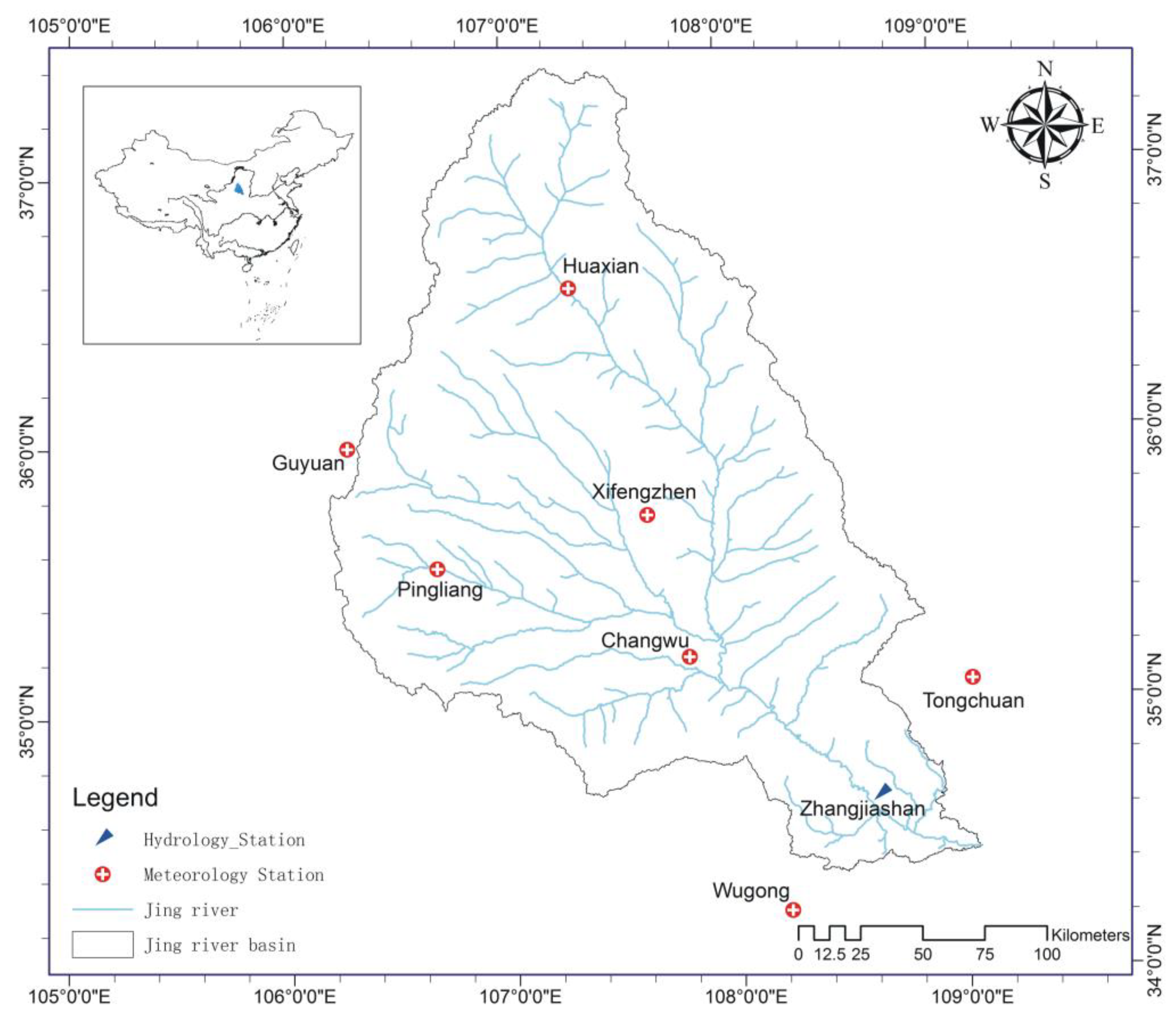
The Jing River, as the largest tributary of the Wei River, originates from the eastern side of the Liupan Mountain in Ningxia Province, China. With a length of 455 km and a basin area of 45.4 × 10³ km2, the Jing River flows from north to south through Pingliang and Changwu Counties, and runs into the Wei River at Gaoling County. The Wei River is approximately 275 km long and has a basin area of approximately 9.24 × 10³ km2 within Shaanxi Province. The drainage basin is located in the middle of the Loess Plateau between 106.2°E–108.7°E and 34.8°N–37.3°N, has a typical temperate continental climate, and is within a semihumid and semiarid area. In the past 60 years, the annual average temperature of the basin has been rising under the influence of the global warming. The annual pan evaporation decreases gradually in the basin, most obviously in the north [40]. The precipitation in the basin decreases from south to north, with an annual average precipitation of 500 mm, which is mainly concentrated in the 6–9 months that accounts for 70% of the annual rainfall. The average annual runoff is 21.4 × 10⁹ m3 in the Jing River Basin, of which 6.02 × 10⁹ m3 reaches Shaanxi Province. It is noted that, under the influence of human activity and climate change, the runoff has decreased significantly in recent decades. Zhangjiashan Station is the hydrological observation section on the main Jing River (Figure 1), at which the measured runoff data can represent the hydrological change in the basin.
It is worth mentioning that the drainage basin is a key area in the “Silk Road Economic Belt” in China. With the potential economic and social development, the water demand in the basin may increase rapidly, which will make it difficult for current regional water resources to meet the demand from economic and social development. Therefore, deeply understanding the changing precipitation and runoff and reasonably allocating water resources are of great significance to the sustainable development of the regional economy and society.
2.2. Data
The precipitation and runoff data used in the study included the monthly runoff data (1960–2012) at Zhang jiashan Station in the Jing River Basin, provided by the Bureau of Hydrology of the Yellow River Water Resources Commission, and the monthly precipitation data (1960–2012) at four meteorological stations (Pingliang, Changwu, Xifengzhen and Guyuan). Monthly sunspot numbers provided by the National Climatic Centre of China [41] were also used. The average precipitation in the basin can be calculated by the Thiessen Polygon approach. The locations of these four meteorological stations and one hydrological station in the basin are shown in Figure 1.
3. Materials and Methods
3.1. Approximate Entropy (ApEn)
ApEn is a nonnegative scalar quantity and is used as a measuring tool of the complexity of a time series. The greater the series’ entropy is, the greater its complexity is. For a time sequence of samples with m dimensions (the length of compared window) and an allowed deviation r(similarity criterion) [42], the ApEn was calculated as follows:
- Step 1.
- Construct a set of vectors with m dimensions:
- Step 2.
- Calculate the Euclidean distance between vectors and :
- Step 3.
- Compute the value of for that isless than r:
- Step 4.
- Take the logarithm of and average the total of over all values of i to obtain:
- Step 5.
- Augment m by1, and repeat steps 1 to 4 to obtain
- Step 6.
- Calculate the ApEnof the time series with m and r:
Equation (6) shows that the ApEn is dependent on m and r. The literature suggests using an n (length of data) larger than 200 and an m of 2, as well as examining several r values before selecting parameters [42]. In this paper, we used , where σ is the standard deviation of x(i). As indicated above, the ApEn reflects the extent of self-similarity between two points in the m dimensional space. The greater the ApEn value, the greater the likelihood that a new IMF created with the same parameters will have the same complexity as the studied sequence. Thus, the ApEn value reflects the system’s ability to maintain its current state under specific conditions.
3.2. Moving Approximate Entropy(M-ApEn)
For a time sequence of samples , we may select a subsequence sequentially through the fixed moving window according to the appropriate step in the original sequence and calculate the ApEn value. The abrupt characteristic of the complexity trend of the original sequence is judged according to the significance of the changes in the ApEn values; the steps are as follows [24,25]:
- Step 1.
- Choose the moving window length h and the moving step size l;
- Step 2.
- Continuously obtain the subsequence with length of h from the ith data (, where n is the total length of sequences);
- Step 3.
- Calculate the ApEn of each subsequence;
- Step 4.
- Slide the window of a fixed size h according to the moving step size l in the original sequence, and repeat steps 2 and 3 until the end of the original sequence;
- Step 5.
- Get an ApEn series;
- Step 6.
- Confirm the abrupt change point of the original sequence according to the trend of the dynamic characteristic values varying with time.
3.3. Bayesian Method
Assuming that the observed value of the hydrological sequence obeys a certain distribution andthe sequence change occurs at a certain point K, the sequence before K is called the front part, shown as , and that after K is called the back part, shown as .While the statistical parameters of the probability distribution of the and are the same, the distribution density functions of and were denoted as follows:
The variance is regarded as a constant in the process, described as . Because both the distribution functions are not known in advance, it is assumed that the distribution functions (a prior distribution) of both and follow the normal distribution, expressed as:
where ( is estimated by the observed value ).
The posterior distribution was derived as follows:
The derivation of the posterior density function of is computed as follows:
- Step 1.
- Given the and ,the joint distribution function of the observed data is derived as follows:
- Step 2.
- According to the Bayes rule, the posterior distribution density function of position K is derived by the following equation:where is the prior distribution for the location of the change point K. Generally, it is assumed to be a uniform distribution, shown as . Under this assumption, the posterior density function of the change point can be simplified as follows:
3.4. Extreme-Point Symmetric Mode Decomposition (ESMD)
The ESMD is the abbreviation for extreme-point symmetric mode decomposition.
For a hydrological sequence data Y = , the ESMD algorithm was represented as follows [32]:
- Step 1.
- Find all the local extreme points (maxima points plus minima points) in the sequence Y and numerate them by with .
- Step 2.
- Connect all the adjacent with line segments, and mark their midpoints by with .
- Step 3.
- Add the left and right boundary midpoints and with a specific approach.
- Step 4.
- Construct p interpolating curves with all these n + 1 midpoints, and calculate their mean value by .
- Step 5.
- Repeat the above four steps on until ( is a permitted error) or the sifting times attain a preset maximum number K. At this point in time, we obtain the first mode .
- Step 6.
- Repeat the above five steps on the residual , and get and , until the last residual R with no more than a certain number of extreme points.
- Step 7.
- Change the maximum number K on a finite integer interval , and repeat the above six steps. Then, calculate the variance of Y− R, and plot a figure with and K, where is the standard deviation of Y.
- Step 8.
- Find the number , which agrees with a minimum on . Then, use the to repeat the previous six steps, and output the whole modes. At this point in time, the last residual R is actually an optimal Adaptive Global Mean (AGM) curve.
4. Results
4.1. Approximate Entropy Variation of Precipitation and Runoff in the Jing River Basin
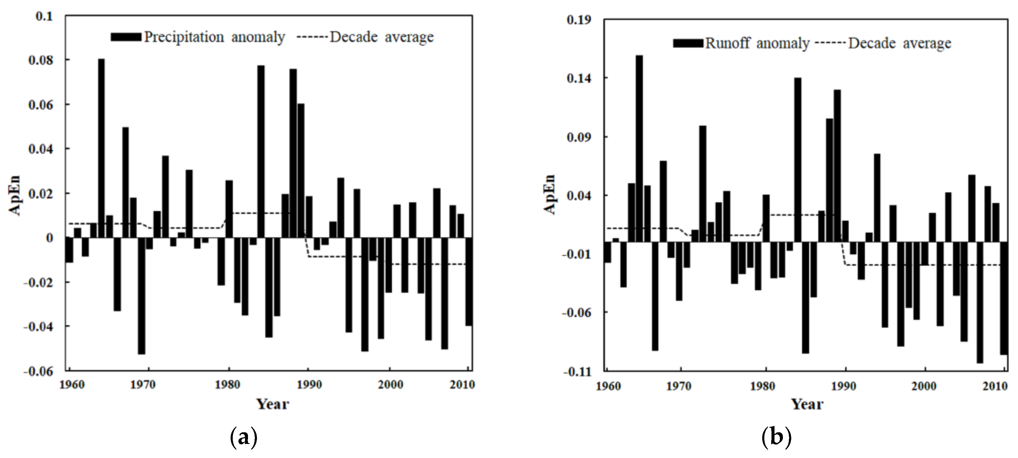
To study the interdecadal variability of the complexity of historical runoff and precipitation, the ApEn values of historical precipitation and runoff per year (n = 365, m = 2, r = 0.15) for the entire study period (1960–2010) and for different decadal periods (1960–1969, 1970–1979, 1980–1989, 1990–1999, and 2000–2010) were calculated and compared. These results are presented in Figure 2.
The ApEn of precipitation and runoff in the Jing River Basin are shown in Figure 2a,b, respectively. The results indicate the decreasing trends of the ApEn decadal changes in the means of both precipitation and runoff. This shows that the complexity of precipitation and runoff decreased. Specifically, the decadal ApEn anomaly variations of precipitation are higher than the long-term average value before the 1990s. However, after the 1990s, this trend is the opposite. The maximum ApEn positive anomalies were found in 1964, 1984 and 1988, while the negative maximum ApEn anomaly followed in 1969, 1985, 1997 and 2007. The moving average curve of ApEn changed once every 10 years, and the reason for this is that the precipitation was heavy and the change of ApEn was complex in the 1960s. In the 1970s, when the climate changed [43] and the precipitation in the basin was relatively lower, the ApEn value decreased. The precipitation began to rise in the 1980s, and the ApEn value increased, but after the 1990s, the basin was in a period of reduced precipitation, and the precipitation ApEn again decreased. For the ApEn of the runoff, as shown in Figure 2b, the change is similar to that of the precipitation: the ApEn anomaly shows two stages before and after 1990; the maximum positive anomalies were found in 1964, 1984 and 1988, and the maximum negative anomaly followed in 1969, 1985, 1997 and 2007.
The above analysis shows that the trend of the complexity of precipitation and runoff is basically consistent, and, as the 1990s progressed, there were obvious changes of precipitation and runoff in the Jing River Basin. The reason for this should be affected by the reduction in precipitation, the increase in water consumption and the growth of terraced fields [44,45]. To date, determining how to deal with this change is an important issue for the rational allocation of water resources in the basin.
4.2. Abrupt Points of Precipitation and Runoff in the Jing River Basin
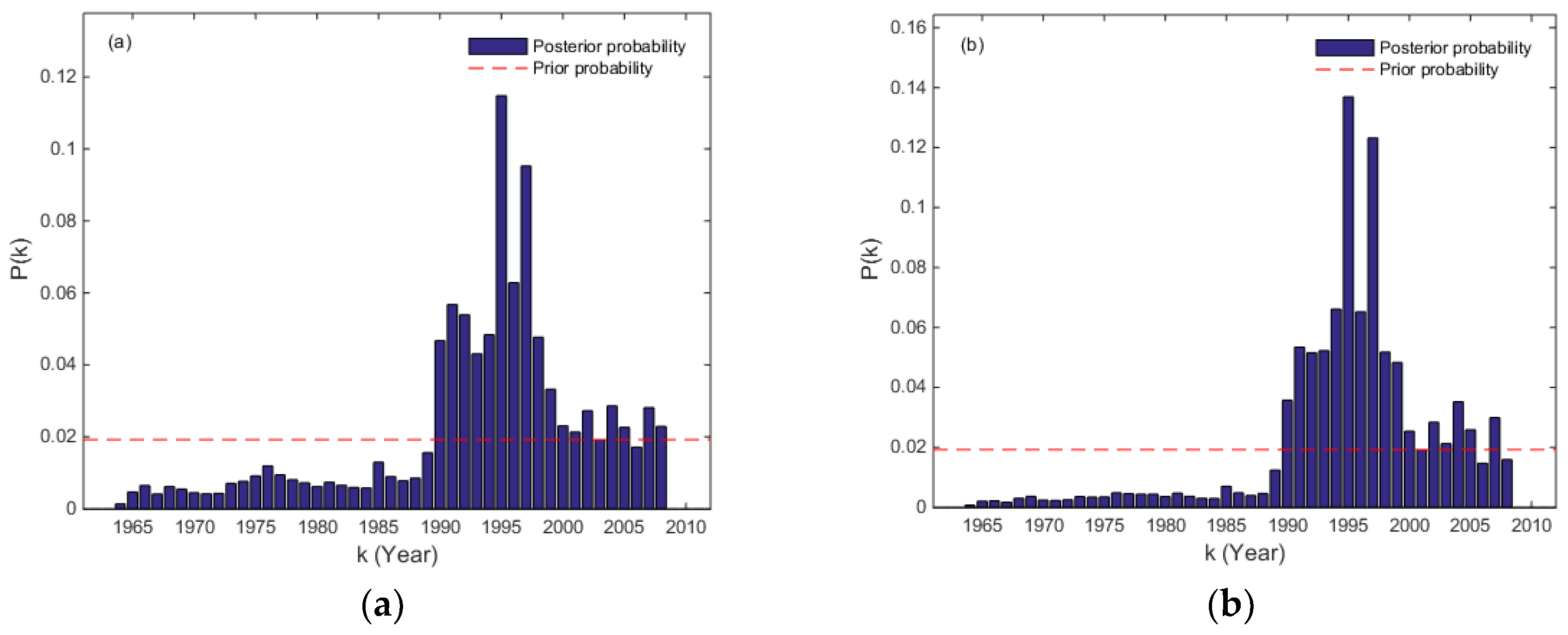
The abrupt changes in precipitation and runoff were analyzed with the Bayesian method. The posterior and prior probabilities of the location of change points Ki for precipitation and runoff are shown in Figure 3.
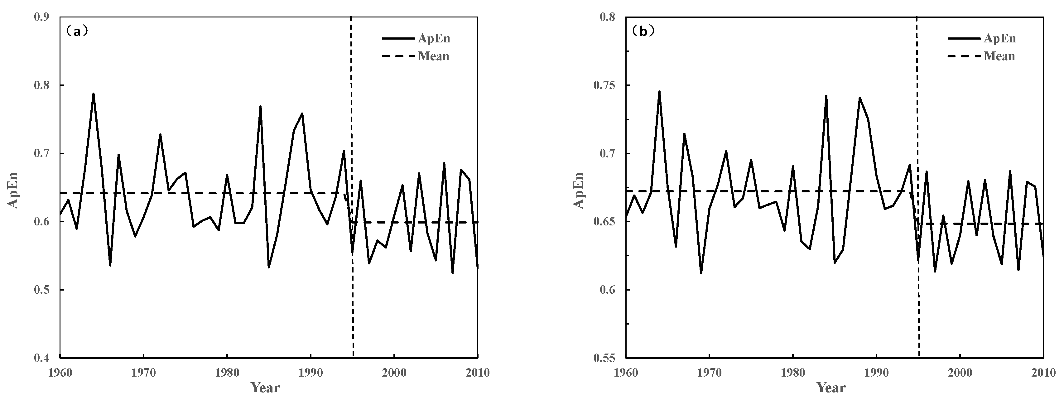
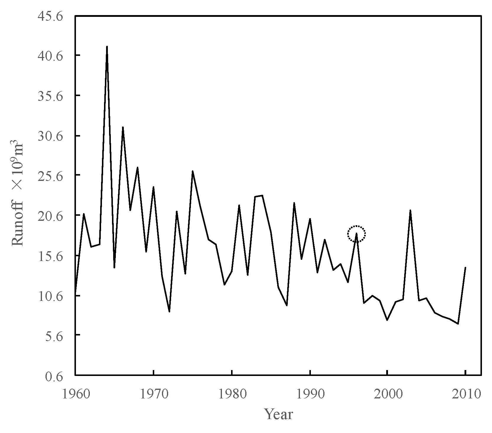
From Figure 3a, it was found that, for the K = 1995 year, the corresponding posterior probability (0.11) is greater, and the Jing River Basin precipitation in 1995 is most likely to change abruptly. In the period of 1960–1995, the mean value of ApEn is 0.64, and the mean value of ApEn is 0.59 during 1995–2010, as shown in Figure 4a, which falls by 7%. Testing the result of the mean differences of the two normal population sat the 5% significance level shows that the changes before and after 1995 were significant. From Figure 3b, it is known that, for the K = 1996 year, the corresponding posterior probability (0.13) is greater. The runoff is most likely to change in 1995 in the Jing River Basin. During 1960–1995, the mean value of ApEn is 0.67, and, in the period of 1995–2010, the mean value of ApEn is 0.64, which falls by 4% (Figure 4b). A T-test analysis result at the 5% significance level shows that the change in the runoff series is also significant. The result is in agreement with the results obtained by Zhao [45] using the Menn-Kendall (MK) method, and in Figure 5, the runoff experienced a significant mutation around 1996 at Zhang jiashan Station. Although a major flood occurred in 2003, the total runoff decreased dramatically after 1996. Considering the published literature, we think that the main reason for the abrupt change is the influence of human activities, such as increasing water consumption, grain for green, natural forest resources protection project and so on [36,46]. During 1991–1996, the river basin was in a continuous dry season. Moreover, the rapid economic development made the industrial and agricultural water use increase sharply. At the same time, the soil and water conservation activities of terrace transformation (slope terrace to horizontal terrace) made the runoff decrease greatly. In 1996, the operation of Zhang jiashan Reservoir (dam filling and sluice storage began in December 1992) caused abrupt changes in runoff and rainfall.
4.3. Approximate Entropy Evolution Analysis of Precipitation and Runoff in the Jing River Basin
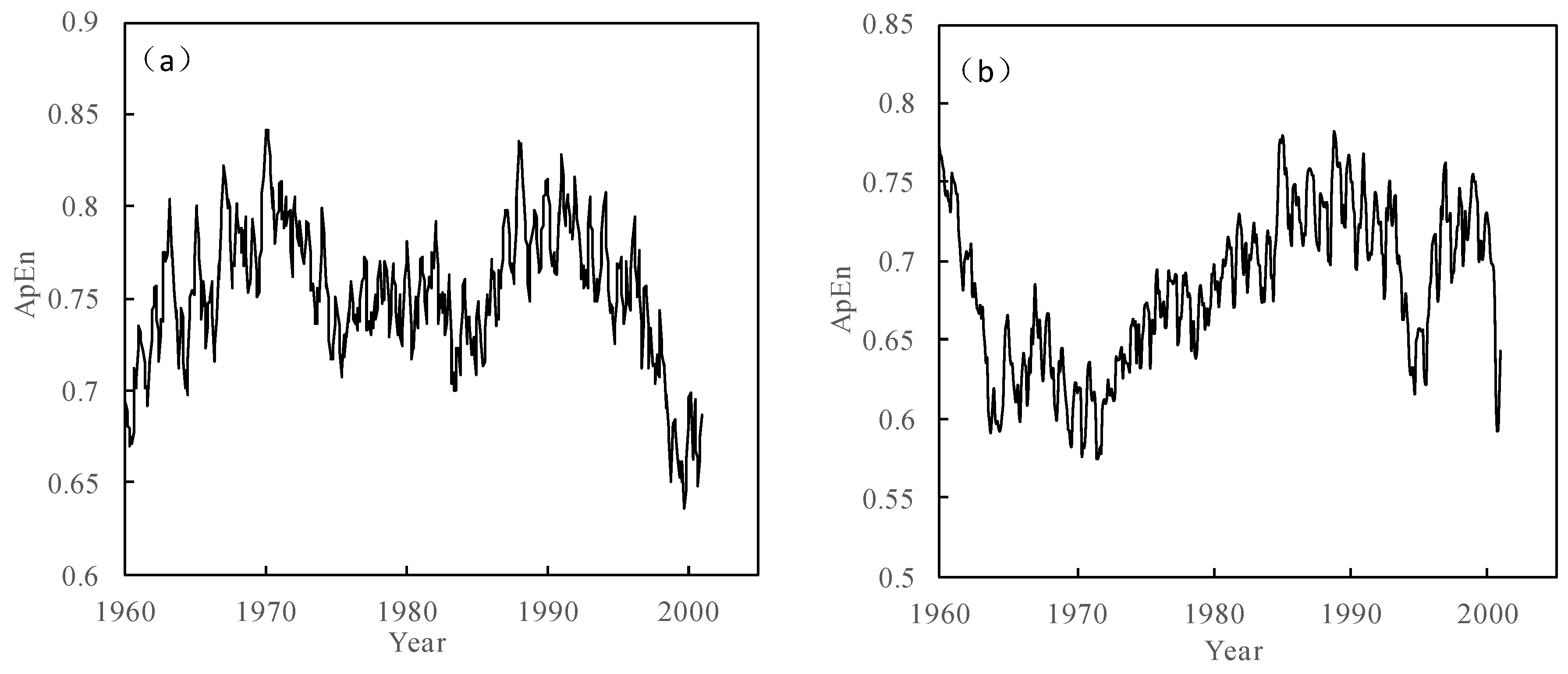
The above-obtained ApEn is a kind of static approximate entropy, which reflects the entire condition of the runoff and precipitation series. To further understand the complexity of the runoff and precipitation series, we calculated the ApEn value of each subsequence with M-ApEn (h = 120 months, l = 1 month, m = 2, ) and assigned it to the last data point of the subsequence. As illustrated in Figure 5, the abscissa x was calculated for the corresponding year by Equation (16):
Year = 1961 + (x/12 − 1)
It is clear from the above-mentioned results that the complexity of the monthly average runoff and precipitation in the Jing River Basin shows various characteristics in different periods. In Figure 6a, the ApEn of precipitation can be roughly divided into three stages: the first stage is before the early 1970s, in which the ApEn showed an upward trend and the complexity of the runoff gradually increased. The second stage is from the 1970s to the middle of the 1980s in which the ApEn was in a state of relative balance. The change occurring in the period should be related to human activities beginning in the 1970s, such as the construction of large area terraces, which changed the underlying surface state of the basin. The third stage is after the 1990s in which the ApEn showed a downward trend.
It is seen from Figure 6b that the ApEn of the runoff shows that the variations declined in the beginning, then rose and finally stabilized. We see that, driven by the abrupt change in climate, the ApEn of the runoff was decreasing and reached the lowest in the early 1970s; it then began to rise and reached its maximum in the early 1990s, in which the second abrupt change in the climate occurred.
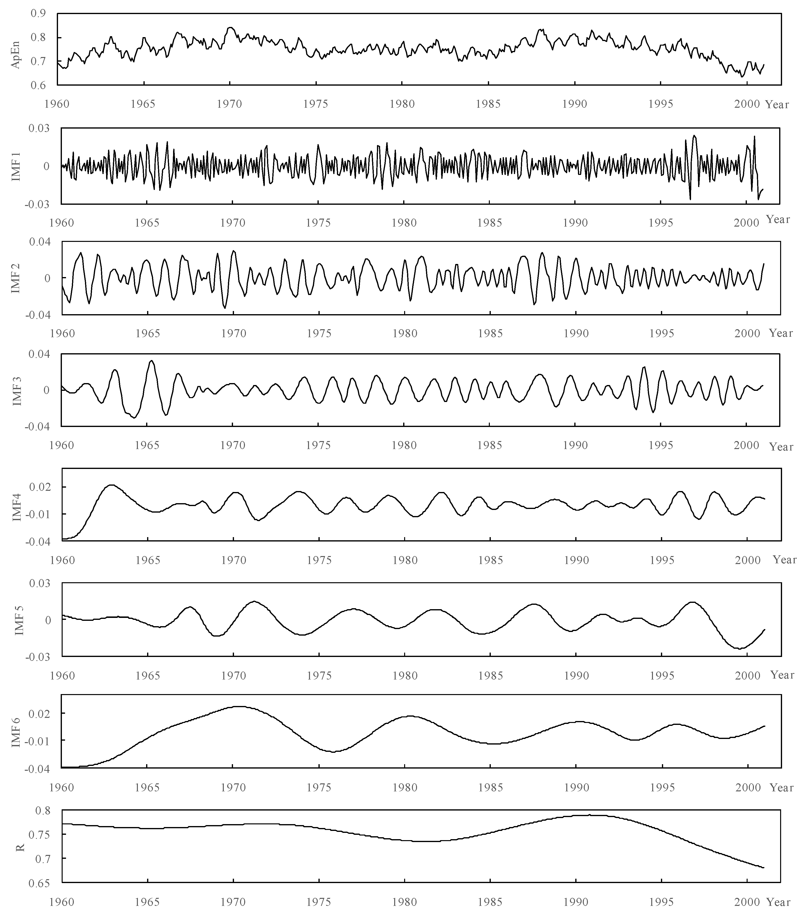
The sunspot activity acts on the climate circulation system through the time-frequency characteristic function, and the climate circulation system transmits the sunspot activity energy, which affects the regional hydrological process (the sunspot activity and the regional hydrological elements have the same change period in multiple time-frequency domains) [47]; for example, the 11-year significant cycles associated with sunspots have been studied in precipitation, runoff and other hydrological processes [48,49,50]. El Niño-Southern Oscillation (ENSO) affects regional hydrological factors by changing the atmospheric circulation, moving rain belt and water vapor transport, and its 2–7-year cycle has a significant impact on precipitation, runoff and other hydrological processes. To further analyze whether precipitation and runoff are affected by a large-scale climate system, as shown in Figure 7 and Figure 8, the ApEn series of monthly precipitation and runoff were stepwise decomposed using the ESMD. It can be seen from Figure 7 that, the ApEn of monthly precipitation was decomposed into six IMF components, and each component represents the ApEn changes at different time scales. The 4–6-year cycle, which is close to ENSO, is clearly shown in the IMF-5 component, and the quasi-decadal cycle closely related to sunspots is clearly shown in the IMF-6 component. The amplitudes of IMF-5 and IMF-6 components had a decreasing trend, and their frequencies increased.
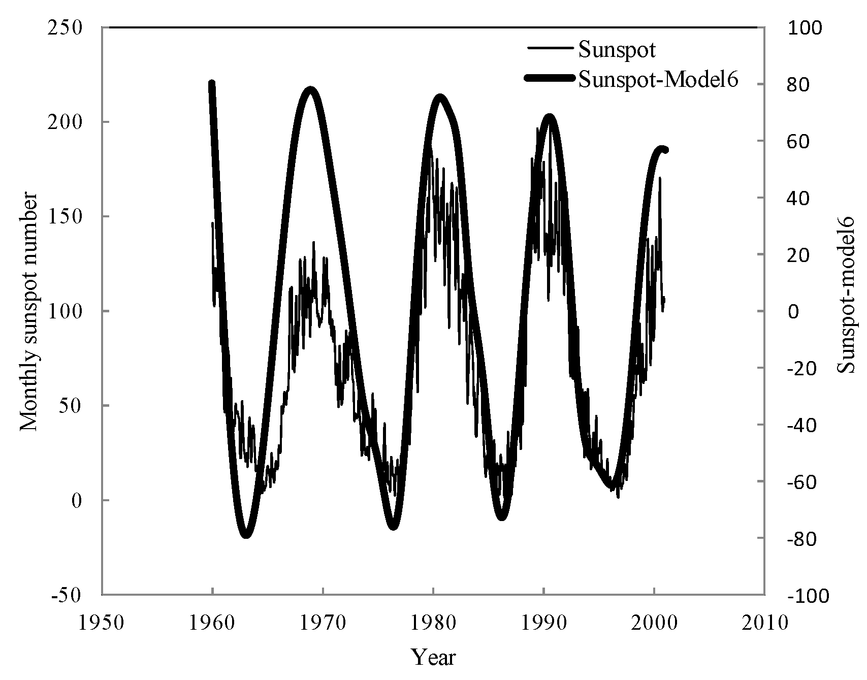
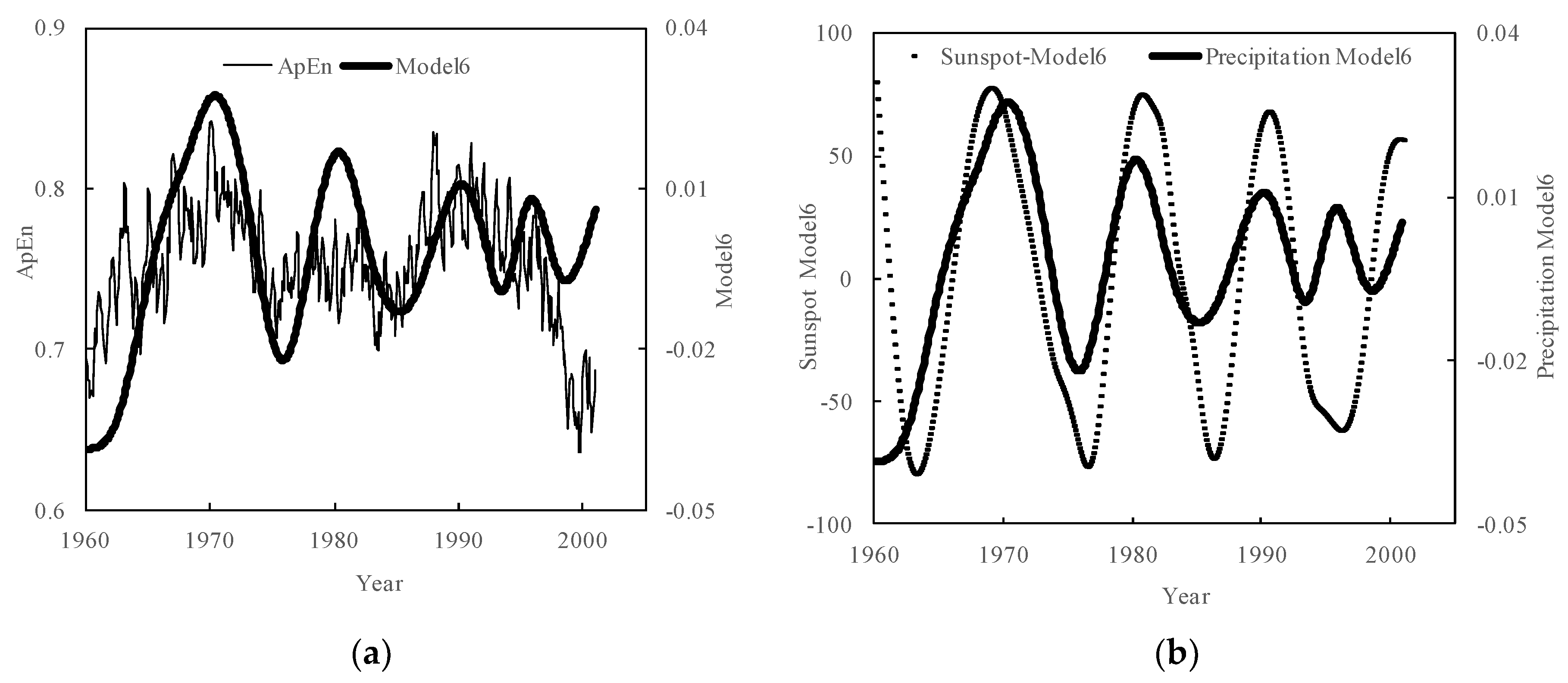
The number of sunspots was also decomposed into the IMF-6 component by ESMD, and it was found that the evolution of IMF-5 component is about the same as that of the sunspots (Figure 9). At the same time, from Figure 10a, it is known that the evolution characteristics of the IMF-6 component are basically the same as the ApEn. Thus, it can be considered that the IMF-6 component shows the mean state of precipitation variation in the Jing River Basin in the recent 50 years. From Figure 10b, the IMF-6 component evolution of precipitation is basically the same as the IMF-6 component evolution of the sunspot numbers, and the correlation coefficient is 0.63.Therefore, it was inferred that sunspots play a leading role in the fluctuation of ApEn, that is, the change in precipitation is mainly influenced by the 10-year quasi-rate of change of the climate cycle. Additionally, it was also seen that 1995 was a shift point. After this point, the amplitude of IMF-6 component decreased and the frequency increased, which further explain why the precipitation changed after 1995.
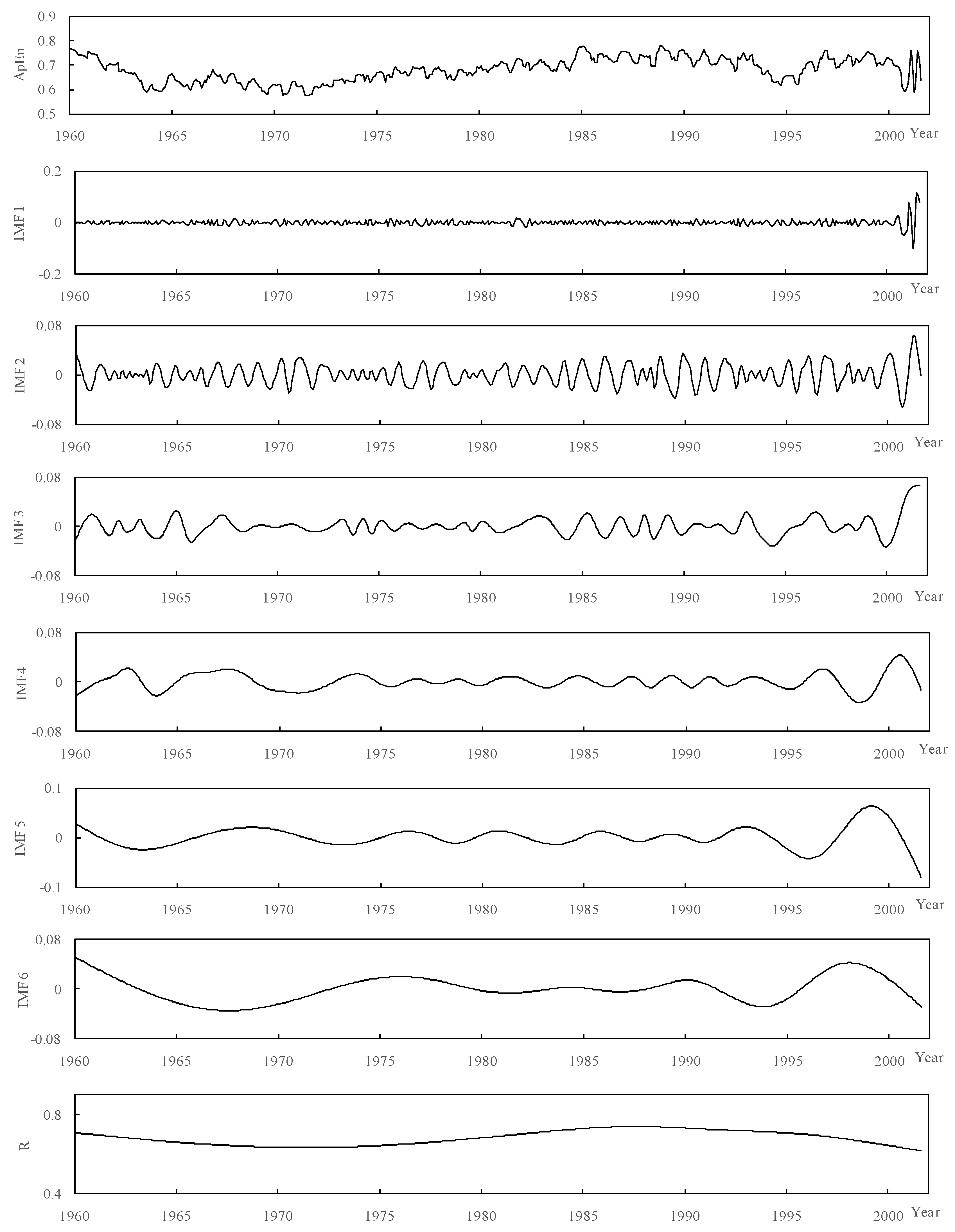
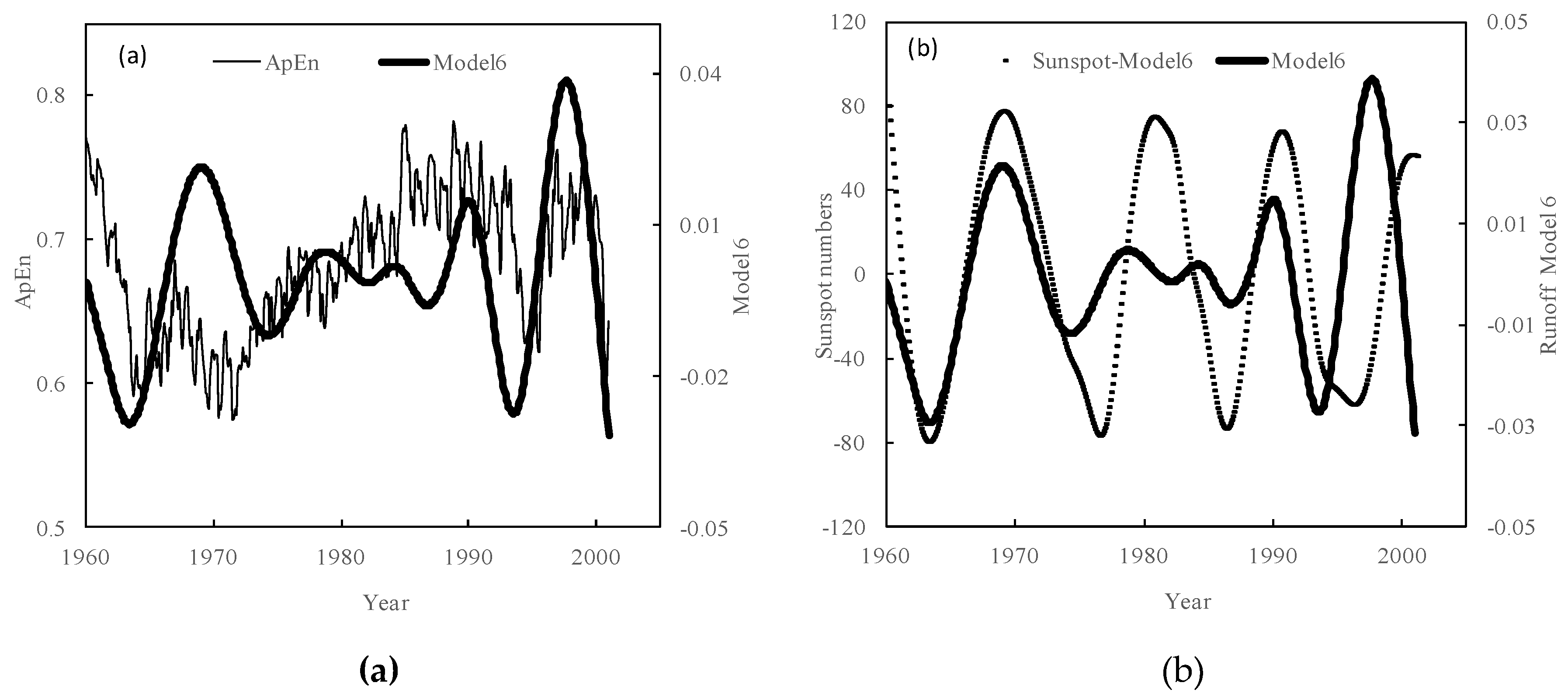
In the same way, the above methods were used to analyze the runoff change. As seen in Figure 11a, the evolution characteristics of the IMF-6 component are basically the same as that of the ApEn. It was then considered that the IMF-6 component indicates the mean state of runoff variation in the Jing River Basin in the recent 50 years. From Figure 11b, we can see that the IMF-6 component was synchronized with sunspot numbers before 1975. However, the amplitude of IMF-6 component decreased and its frequency increased after 1975, which began to diverge from the status of the IMF-6 component of sunspot numbers before 1975. The correlation coefficient is only 0.41. The change shows that the runoff was affected by human activity in the 1970s. Some water and soil conservation projects (terraced fields, silt dams and reservoirs and so on), which had been implemented, as well as vegetation restoration and the afforestation of barren hills, began to have obvious influences on the drainage area. Unlike the situation in the 1970s, urban expansion, industrial growth, agricultural irrigation, etc. became the dominant factors and further reduced runoff in the 1980s. In the 1990s, the large-scale structural adjustment of terraced fields (such as slope terraced fields to level terraces) began to have more impacts on the generation of runoff [51]. Overall, these human factors make the past changes in runoff more complex and destroy the consistency of the hydrological sequence, which brings some difficulties to watershed hydrological analysis.
The correlation coefficient between precipitation and sunspot is 0.63, and the coefficient between runoff and sunspot is 0.41. The reason may be that the regional precipitation change is mainly affected by large-scale climate factors, and is relatively less affected by human activities. In the process of runoff formation, it is not only affected by precipitation, but also by the underlying surface conditions (topography, vegetation and river network) of the basin. There is a good correlation between natural falling water and runoff, but under the influence of human activities, the underlying surface of the basin has changed, changing the proportion of climate factors and human activities in the process of runoff formation. The proportion of human activities was increasing, so the correlation coefficient between precipitation and sunspots is significantly higher than runoff.
5. Conclusions
In this study, based on precipitation and runoff data of the Jing River Basin from 1960 to 2010, the complexity of the precipitation and runoff was analyzed by ApEn. The abrupt change points in the precipitation and runoff series were examined by the Bayesian method, and the multitime scales characteristics of precipitation and runoff were also discussed. The major conclusions are as follows:
- (1)
- The ApEn variation shows that the evolution of the complexity of precipitation and runoff is basically consistent: the decadal variations of both precipitation and runoff are characterized by periodic fluctuations; there was a very obvious decrease when it entered the 1990s; the ApEn values in the periods1960–1970, 1970–1980, and1980–1990 are higher than the long-term average value, while they are lower than the long-term average value in the periods1990–2000 and 2000–2010.
- (2)
- The Bayesian analysis shows that abrupt changes occurred in the precipitation and runoff in 1995. The T-test analysis result at the 5% significance level shows that the abrupt changes are significant. Based on previous literature, the increase in water consumption and the implementation of water conservation measures are considered to be the main reasons causing these variations. Additionally, more attention needs to be paid to the abrupt changes, which will have a direct impact on the analysis of hydrological consistency in the future.
- (3)
- Based on the results of the ESMD, the change of precipitation is related with ENSO and sunspots on large time scales. There is a close relationship between the precipitation and the sunspot activity (a ten-year quasi-cycle), and the correlation coefficient is 0.63, indicating that the sunspot activity may play a leading role in the evolution of precipitation. However, we also found that the correlation coefficient between the runoff and sunspots is only 0.41, indicating that the climate change rate is not the dominant factor of runoff change and that runoff change would be affected synthetically by climate change and other factors.
Author Contributions
All authors contributed to this study. D.S. provided the writing idea, carried out data analyses and drawing, and wrote the first draft of the manuscript. Z.G. contributed to the analysis of results. H.Z. revised the manuscript and supervised the study. All authors read and approved the final manuscript.
Funding
Project supported by the National Natural Science Foundation of China (Grant No. 51409005 and 51379014), the Fundamental Research Funds for the Central Universities (Grant No. 300102298103), the Technology Foundation for Selected Overseas Chinese Scholars, Department of Personnel in Shaanxi Province of China (Grant No. 2017035), the Natural Science Foundation of Hebei Province (Grant No.E2016402098), and the Science and Technology Research Project of Hebei Colleges and Universities (Grant No.QN2015253).
Conflicts of Interest
The authors declare no conflict of interest.
Abbreviations
The following abbreviations are used in this manuscript:
| ApEn | Approximate Entropy |
| EMD | Empirical Mode Decomposition |
| ESMD | Extreme-point Symmetric Mode Decomposition |
| M-ApEn | Moving Approximate Entropy |
| IMF | Intrinsic Mode Function |
References
- Allen, M.R.; Ingram, W.J. Constraints on future changes in climate and the hydrologic cycle. Nature 2002, 419, 224–232. [Google Scholar] [CrossRef] [PubMed]
- Liu, Y.Y.; Zhang, X.N.; Xia, D.Z.; Bakir, M. Impacts of land-use and climate changes on hydrologic processes in the Qingyi River Watershed, China. J. Hydrol. Eng. 2011, 18, 1495–1512. [Google Scholar] [CrossRef]
- Dunn, S.M.; Brown, I.; Sample, J.; Post, H. Relationships between climate, water resources, land use and diffuse pollution and the significance of uncertainty in climate change. J. Hydrol. 2012, 434–435, 19–35. [Google Scholar] [CrossRef]
- Chang, J.X.; Zhang, H.X.; Wang, Y.M.; Zhu, Y.L. Assessing theimpact of climate variability and human activities on streamflow variation. Hydrol. Earth. Syst. Sci. 2016, 20, 1547–1560. [Google Scholar] [CrossRef]
- Wang, W.S.; Huang, W.J.; Ding, J. Study on the complexity of runoff change based on the dis-noisingof wavelet transform and symbolic dynamics. Adv. Water Sci. 2005, 16, 380–383. [Google Scholar]
- Tong, C.S.; Huang, Q.; Liu, H. Analysis on runoff time series dynamics character based on complexity theory. Syst. Eng. Theory Pract. 2004, 24, 102–107. [Google Scholar]
- Chou, C.M. Complexity analysis of rainfall and runoff time series based on sample entropy in different temporal scales. Stoch. Environ. Res. Risk Assess. 2014, 28, 1401–1408. [Google Scholar] [CrossRef]
- Teixeira, A.; Matos, A.; Souto, A.; Antunes, L. Entropy measures vs. Kolmogorov complexity. Entropy 2011, 13, 595–611. [Google Scholar] [CrossRef]
- Xia, J.; Shang, P.; Wang, J.; Shi, W. Permutation and weighted-permutation entropy analysis for the complexity of nonlinear time series. Commun. Nonlinear Sci. 2012, 31, 60–68. [Google Scholar] [CrossRef]
- Mikhailovsky, G.E.; Levich, A.P. Entropy, information and complexity or which aims the arrow of time? Entropy 2015, 17, 4863–4890. [Google Scholar] [CrossRef]
- Zhang, L.; Singh, V.P. Bivariate rainfall and runoff analysis using entropy and copula theories. Entropy 2014, 14, 1784–1812. [Google Scholar] [CrossRef]
- Rahimi, A. Probability distribution of rainfall-runoff using entropy theory. Trans. Asabe 2012, 55, 1733–1744. [Google Scholar]
- Wrzesiński, D. Use of Entropy in the Assessment of Uncertainty of River Runoff Regime in Poland. ActaGeophys. 2016, 64, 1825–1839. [Google Scholar] [CrossRef]
- Pincus, S.M.; Goldberger, A.L. Physiological time-series analysis: What does regularity quantify? Am. J. Physiol. 1994, 266, H1643–H1656. [Google Scholar] [CrossRef] [PubMed]
- Pincus, S.M. Approximate entropy (ApEn) as a complexity measure. Chaos 1995, 5, 110–117. [Google Scholar] [CrossRef] [PubMed]
- Bruhn, J.; Röpcke, H.; Hoeft, A. Approximate entropy as an electroencephalographic measure of anesthetic drug effect during desflurane anesthesia. Anesthesiology 2000, 92, 715–726. [Google Scholar] [CrossRef] [PubMed]
- West, J.; Lacasa, L.; Severini, S.; Teschendorff, A. Approximate entropy of network parameters. Phys. Rev. E 2012, 85. [Google Scholar] [CrossRef] [PubMed]
- Fan, J.J.; Huang, Q.; Chang, J.X.; Sun, D.Y.; Cui, S. Detecting abrupt change of streamflow at Lintong Station of Wei River. Math. Probl. Eng. 2013. [Google Scholar] [CrossRef]
- Wu, H.T.; Yang, C.C.; Lin, G.M.; Haryadi, B.; Chu, S.C.; Yang, C.M.; Sun, C.K. Multiscale cross-approximate entropy analysis of bilateral fingertips photoplethysmographic pulse amplitudes among middle-to-old aged individuals with or without type 2 diabetes. Entropy 2017, 19, 1–10. [Google Scholar] [CrossRef]
- Gong, M.C.; Kawahito, Y.; Li, G.; Gao, M.; Zeng, X.Y. Stabilization effect of space constraint in narrow gap laser-arc hybrid welding analyzed by approximate entropy. Int. Adv. Manuf. Technol. 2017, 92, 3093–3102. [Google Scholar] [CrossRef]
- Li, X.G.; Wei, N.; Wei, X. Complexity analysis of precipitation-runoff series based on a new parameter-optimization method of entropy. J. Hydrol. Eng. 2017, 22, 1–10. [Google Scholar] [CrossRef]
- Liu, D.F.; Tian, F.Q.; Huang, Q.; Lin, M. Analysis of the dynamics of ecohydrological system in the river basin. J. Xi'an Univ. Technol. 2013, 29, 379–385. [Google Scholar]
- Tong, C.S.; Liu, H.; Huang, Q.; Xue, X.J. The analyze of the rivers and runoff evolution feature on the basis of complexity theory. Dyn. Contin. Discret. Impuls. Syst. Ser. A Math. Anal. 2006, 13, 917–920. [Google Scholar]
- Wang, Q.G.; Zhang, Z.P. The research of detecting abrupt climate change with approximate entropy. Acta Phys. Sin. 2008, 57, 1976–1983. [Google Scholar]
- Sun, D.Y.; Qiang, H.; Wang, Y.M.; Liu, Z.; Zhang, L. Application of moving approximate entropy to mutation analysis of runoff time series. J. Hydrol. Eng. 2014, 33, 1–6. [Google Scholar]
- He, W.P.; Wu, Q.; He, T.; Cheng, H.Y.; Zhang, W.; Wu, Q. A new method to detect abrupt change based on approximate entropy. Acta Phys. Sin. 2011, 60, 049202. [Google Scholar]
- Jin, H.M.; He, W.P.; Hou, W. Effects of different trends on moving cut data-approximate entropy. Acta Phys. Sin. 2012, 61, 069201. [Google Scholar]
- Rudi, J.; Pabel, R.; Jager, G.; Koch, R.; Kunoth, A.; Bogena, H. Multiscale analysis of hydrologic time series data using the Hilbert-Huang transform. Vadose Zone J. 2010, 9, 925–942. [Google Scholar] [CrossRef]
- Karthikeyan, L.; Kumar, D.N. Predictability of nonstationary time series using wavelet and EMD based ARMA models. J. Hydrol. 2013, 502, 103–119. [Google Scholar] [CrossRef]
- Kisi, O.; Latifoğlu, L.; Latifoğlu, F. Investigation of empirical mode decomposition in forecasting of hydrological time series. Water Resour. Manag. 2014, 28, 4045–4057. [Google Scholar] [CrossRef]
- Wu, Z.H.; Huang, N.E. Ensemble empirical mode decomposition: A noise-assisted data analysis method. Adv. Adapt. Data Anal. 2011, 1, 1–41. [Google Scholar] [CrossRef]
- Wang, T.; Zhang, M.C.; Yu, Q.H.; Zhang, H.Y. Comparing the application of EMD and EEMD on time-frequency analysis of seimic signal. J. Appl. Geophys. 2012, 83, 29–34. [Google Scholar] [CrossRef]
- Wang, J.L.; Li, Z.J. Extreme-point symmetric mode decomposition method for data analysis. Adv. Adapt. Data Anal. 2013, 5, 1350015. [Google Scholar] [CrossRef]
- Li, H.F.; Wang, J.L.; Li, Z.J. Application of ESMD method to air-sea flux investigation. Int. J. Geosci. 2013, 4, 8–11. [Google Scholar] [CrossRef]
- Lei, J.R.; Liu, Z.H.; Bai, L.; Chen, Z.S.; Xu, J.H.; Wang, L.L. The regional features of precipitation variation trends over Sichuan in China by the ESMD method. Mausam 2016, 67, 849–860. [Google Scholar]
- Liu, X.L.; Tang, Y.; Lu, Z.; Huang, H.; Tong, X.H.; Mang, J. ESMD-based stability analysis in the progressive collapse of a building IMF: A case study of a reinforced concrete frame-shear wall IMF. Measurement 2018, 120, 34–42. [Google Scholar] [CrossRef]
- Guo, A.J.; Chang, J.X.; Wang, Y.M.; Li, Y.Y. Variation characteristics of rainfall-runoff relationship and driving factors analysis in Jinghe River Basin in nearly 50 years. Trans. Chin. Soc. Agric. Eng. 2015, 31, 165–171. [Google Scholar]
- Xu, L.H.; Shi, Z.J.; Wang, Y.H.; Wang, Y.N. Spatiotemporal variation and driving forces of reference evapotranspiration in Jing River Basin, northwest China. Hydrol. Processes 2015, 29, 4846–4862. [Google Scholar] [CrossRef]
- He, Y.; Wang, F.; Mu, X.M.; Yan, H.; Zhao, G.J. An assessment of human versus climatic impacts on Jing River Basin, loess plateau, China. Adv. Meteorol. 2015, 478739, 1–13. [Google Scholar] [CrossRef]
- Wang, P.; Qiu, G.Y.; Yin, J.; Xiong, Y.J.; Xie, F. Spatial distribution and temporal trend of temperature and pan evaporation in Jinghe River Basin. Arid Meteorol. 2008, 26, 17–22. [Google Scholar]
- China Meteorological Administration. Climatic Data Center, National Meteorological Information Center. Available online: http://cma.gov.cn/ (accessed on 16 May 2018).
- Yentes, J.M.; Hunt, N.; Schmid, K.K.; Kaipust, J.P.; Grath, D.M.; Stergiou, N. The appropriate use of approximate entropy and sample entropy with short data sets. Ann. Biomed. Eng. 2013, 41, 349–365. [Google Scholar] [CrossRef] [PubMed]
- Shi, N.; Chen, J.Q. 4-phase climate change features in the last 100 years over China. Acta Meteorol. Sin. 1995, 53, 431–439. [Google Scholar]
- Xie, F.; Qiu, G.Y.; Yin, J.; Xiong, Y.J.; Wang, P. Comparison of landuse/land cover change in three sections of the Jinghe RiverBasin between the 1970–2006. J. Nat. Resour. 2009, 24, 1344–1365. [Google Scholar]
- Zhu, H.Y.; Han, C.B.; Jia, Z.F.; Liu, Y.; Li, P.C. Analysis oncharacteristics of runoff and sediment of Zhangjiashanhydrological station and case study for Jinghe River. Trans. Chin. Soc. Agric. Eng. 2012, 28, 48–55. [Google Scholar]
- Zhao, J.; Huang, Q.; Chang, J.X.; Liu, D.F.; Huang, S.Z.; Shi, X.Y. Analysis of temporal and spatial trends of hydro-climatic variables in the Wei River Basin. Environ. Res. 2015, 139, 55–64. [Google Scholar] [CrossRef] [PubMed]
- Dong, L.Y.; Zhang, P.C.; Liu, J.G.; Tong, X.X.; Xie, H. Combined influence of solar activity and ENSO on hydrological processes in Yoshino River basin, Japan. Adv. Water Sci. 2017, 5, 671–680. [Google Scholar]
- Hiremath, K.M. The influence of solar activity on the rainfall over India: Cycle-to-cycle variations. J. Astrophys. Astron. 2006, 27, 367–372. [Google Scholar] [CrossRef] [Green Version]
- Qian, Z. Influence of solar activity on the precipitation in the North-central China. New Astron. 2017, 51, 161–168. [Google Scholar]
- Fu, C.; James, A.L.; Wachowiak, M.P. Analyzing the combined influence of solar activity and El Niño on streamflow across southern Canada. Water. Resour. Res. 2012, 48, W05507–W05525. [Google Scholar] [CrossRef]
- Zhang, S.L.; Wang, Y.H.; Yu, P.T.; Zhang, H.J.; Tu, X.W. Study for Separating the impact of precipitation variation and human activities on runoff change of the upper reaches of Jing River. J. Soil Water Conserv. 2010, 24, 53–58. [Google Scholar]
Figure 1.
The locations of the hydrological and meteorological stations in the Jing River Basin.

Figure 2.
The annual approximate entropy (ApEn) of precipitation (a) and runoff (b) with the differences of their decadal mean values in the Jing River Basin.
Figure 2.
The annual approximate entropy (ApEn) of precipitation (a) and runoff (b) with the differences of their decadal mean values in the Jing River Basin.

Figure 3.
The abrupt Bayesian analysis of precipitation (a) and runoff (b).

Figure 4.
The ApEn of monthly mean precipitation (a) and runoff (b).

Figure 5.
The runoff of Zhangjiashan Station.

Figure 6.
The moving approximate entropy (M-ApEn) of monthly mean precipitation (a) and runoff (b), (h = 120 months, l = 1 month, m = 2, ).
Figure 6.
The moving approximate entropy (M-ApEn) of monthly mean precipitation (a) and runoff (b), (h = 120 months, l = 1 month, m = 2, ).

Figure 7.
The Intrinsic Mode Function (IMF) components of precipitation ApEn by extreme-point symmetric mode decomposition (ESMD).
Figure 7.
The Intrinsic Mode Function (IMF) components of precipitation ApEn by extreme-point symmetric mode decomposition (ESMD).

Figure 8.
The IMF components of runoff ApEn by ESMD.

Figure 9.
The monthly sunspot numbers and IMF-6 component.

Figure 10.
The comparisons between the precipitation ApEn and IMF-6component (a) as well as between the IMF-6 component of sunspot numbers and IMF-6 component of precipitation (b).
Figure 10.
The comparisons between the precipitation ApEn and IMF-6component (a) as well as between the IMF-6 component of sunspot numbers and IMF-6 component of precipitation (b).

Figure 11.
The comparisons between the runoff ApEn and IMF-6 component (a) as well as between the IMF-6 component of sunspot numbers and IMF-6 component of runoff (b).
Figure 11.
The comparisons between the runoff ApEn and IMF-6 component (a) as well as between the IMF-6 component of sunspot numbers and IMF-6 component of runoff (b).

© 2018 by the authors. Licensee MDPI, Basel, Switzerland. This article is an open access article distributed under the terms and conditions of the Creative Commons Attribution (CC BY) license (http://creativecommons.org/licenses/by/4.0/).
Share and Cite
MDPI and ACS Style
Sun, D.; Zhang, H.; Guo, Z. Complexity Analysis of Precipitation and Runoff Series Based on Approximate Entropy and Extreme-Point Symmetric Mode Decomposition. Water 2018, 10, 1388. https://0-doi-org.brum.beds.ac.uk/10.3390/w10101388
AMA Style
Sun D, Zhang H, Guo Z. Complexity Analysis of Precipitation and Runoff Series Based on Approximate Entropy and Extreme-Point Symmetric Mode Decomposition. Water. 2018; 10(10):1388. https://0-doi-org.brum.beds.ac.uk/10.3390/w10101388
Chicago/Turabian StyleSun, Dongyong, Hongbo Zhang, and Zhihui Guo. 2018. "Complexity Analysis of Precipitation and Runoff Series Based on Approximate Entropy and Extreme-Point Symmetric Mode Decomposition" Water 10, no. 10: 1388. https://0-doi-org.brum.beds.ac.uk/10.3390/w10101388
Note that from the first issue of 2016, this journal uses article numbers instead of page numbers. See further details here.