Multi-Crop Production Decisions and Economic Irrigation Water Use Efficiency: The Effects of Water Costs, Pressure Irrigation Adoption, and Climatic Determinants

Abstract

In an irrigated multi-crop production system, farmers make decisions on the land allocated to each crop, and the subsequent irrigation water application, which determines the crop yield and irrigation water use efficiency. This study analyzes the effects of the multiple factors on farmers’ decision making and economic irrigation water use efficiency (EIWUE) using a national dataset from the USDA Farm and Ranch Irrigation Survey. To better deal with the farm-level data embedded in each state of the U.S., multilevel models are employed, which permit the incorporation of state-level variables in addition to the farm-level factors. The results show higher costs of surface water are not effective in reducing water use, while groundwater costs show a positive association with water use on both corn and soybean farms. The adoption of pressure irrigation systems reduces the soybean water use and increases the soybean yield. A higher EIWUE can be achieved with the adoption of enhanced irrigation systems on both corn and soybean farms. A high temperature promotes more the efficient water use and higher yield, and a high precipitation is associated with lower water application and higher crop yield. Intraclass correlation coefficients (ICC) suggest a moderate variability in water application and EIWUE is accounted by the state-level factors with ICC values greater than 0.10.

1. Introduction

In many countries, agricultural production relies heavily on water resources [1]. Most of the cropland is irrigated and some traditionally rain-fed agriculture systems have seen growing irrigation to increase production and mitigate climate risks. Accounting for more than 80–90% of the total water withdrawals, irrigated agriculture needs to contribute an increasing share of food production to meet the growing demands of a rising population [2]. Faced with the dramatic impacts of climate change, many arid and semiarid areas are suffering from severe water shortages, for instance, the Western U.S. [3] and Northwestern China [4]. At the same time, some areas that were not facing water deficiencies are experiencing more, frequent droughts, for instance, the Midwestern U.S. [5,6], thus, increasing the stress on current water resources. In addition, in many areas, the water demand from other sectors is expected to grow faster. Though a large proportion of water demand could be satisfied through new investments in water supply and irrigation systems, and the expansion of water supply could be met with some non-traditional sources, the shrinking water availability increases both economic and environmental costs of developing new water supplies [2,7,8]. Therefore, investments in water systems and developing new water sources to meet growing demands will not be a sufficient solution.

As a more practical path to achieve the sustainability of water resources, water can be saved in current uses through increasing the irrigation water use efficiency (total yield per unit of land divided by irrigation water applied) in agricultural production [9]. The traditional flood (also called furrow or gravity) irrigation systems have been reported to lose 50–70% of the water applied as soil evaporation, seepage, and deep drainage [10,11]. Potential improvements in irrigation water use efficiency can be realized by adopting enhanced pressure irrigation systems.

Most of the studies on irrigation water use efficiency are conducted at the field level based on experiments [12,13]. Two foci of field experiments include the comparison of irrigation water use efficiency at different water application levels and utilizing various irrigation methods, and the interaction and compatibility of improved irrigation systems and other farm-related management practices that are considered the best (e.g., film or straw mulching, irrigation scheduling, and soil testing) [14,15,16,17]. Previous studies on irrigation water use efficiency (IWUE) typically used experimental data in one field, collected over multiple years. Because of limited research funding, heterogeneity of experimental fields, and the diversity of cropping systems and farming structures, the available farm-level data are limited. As a result, the evaluation of crop IWUE in multiple fields is very challenging. At the farm level, producers usually plant two or more crops in one growing season. In addition to making adoption decisions regarding different irrigation systems, farmers also need to make decisions on land allocation and irrigation water application for each crop that they choose to plant. These decisions can determine whether the water is used efficiently or not.

The farm-level irrigation and production decisions to improve irrigation efficiency in a multi-crop system are understudied, in particular, across regions with different cropping patterns and climatic conditions [18]. In addition, production decisions in irrigated agriculture may be affected by other factors like water sources, input costs, and the farming area [19]. Analysis of irrigation decisions and crop irrigation water use efficiency, as affected by these and other factors, could help farmers and policymakers adapt to potential climate risks, better manage the irrigation water application, and achieve the sustainable use of limited water resources. Furthermore, given the heterogeneity of farms and states, multi-level models (MLMs) can be readily utilized to deal with the hierarchical nature of the farm-level data and to extract the percentage of variability in each response accounted for by farm- and state-level factors. The multilevel model has been applied in social science research [20,21] and agricultural sciences. To analyze the hierarchically structured data, Neumann et al. [22] adopted the multilevel model to investigate the global irrigation patterns using country-level data, and Giannakis and Bruggeman [23] studied the labor productivity in agricultural system in Europe. However, MLMs have never been used to analyze crop production decisions or farm irrigation efficiency. Given the data structure of the United States Department of Agriculture Farm and Ranch Irrigation Survey (USDA FRIS)—i.e., farms are embedded in states—we explore the applicability of the MLMs to multiple equations relating to production decisions in irrigated multi-crop agriculture.

Therefore, the objective of this study is to better understand the production decisions for irrigated agriculture and economic irrigation water use efficiency of major crops in the U.S., as well as the effects of water costs, the adoption of pressure irrigation systems, and the climatic determinants in a multi-crop production system.

Specifically, this research aims to answer the following fundamental questions:

(1)

Are enhanced irrigation systems conserving water and are they more efficient than the traditional systems under diverse farm conditions?

(2)

How does climate variability affect production decisions in an irrigated agriculture?

(3)

What are the major influential factors and how are the multi-crop production decisions affected by these factors at the farm and state levels?

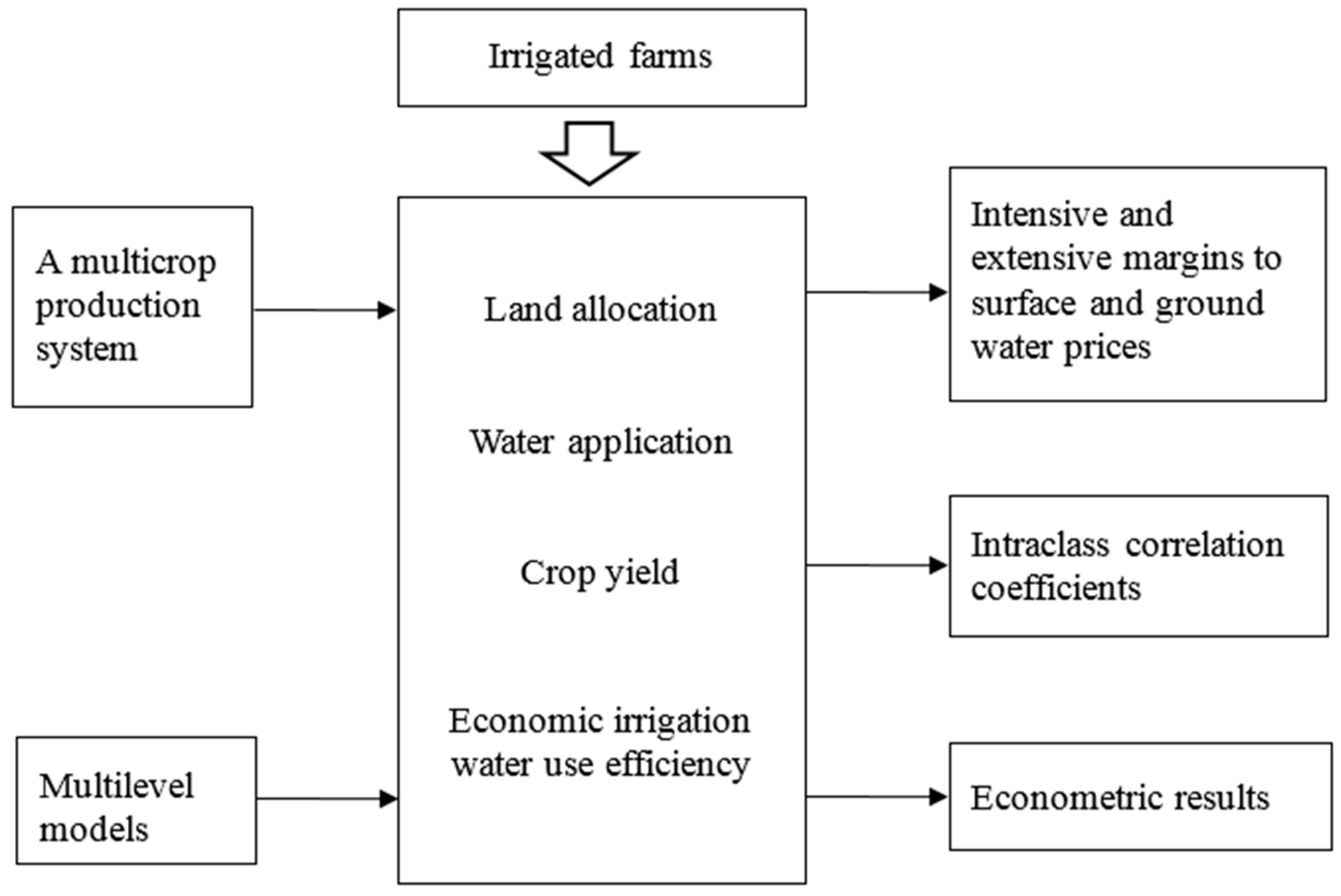
The layout of the analyses in this paper is presented in Figure 1. Focusing on irrigated farms in a multi-crop production system, four equations on land allocation, water application, crop yield, and economic irrigation water use efficiency are estimated using multilevel models. Intensive and extensive margins of water use to water price and energy costs are calculated. Intraclass correlation coefficients (ICC) as defined later are calculated to find out the proportion of variability in each response is accounted for by each level. Econometric results from the multilevel models are provided to show the effects of exogenous variables on each response variable.

2. Literature Review

Crop Water Use Efficiency

In general, water management includes issues relating to five sub-systems existing on most irrigated farms: supply systems, on-farm storage systems, on-farm distribution systems, application systems, and recycling systems [11]. In a report on the Australian cotton industry, Dalton et al. [11] defined water use efficiency at the farm level by focusing on three dimensions: agronomic efficiency, economic efficiency, and volumetric efficiency. The agronomic water use efficiency includes a gross production water use index (yield/total water applied), an irrigation water use index (yield/irrigation water applied), a marginal irrigation water use index (marginal yield due to irrigation/irrigation water applied), and a crop water use index (yield/evapotranspiration). The economic water use efficiency includes a gross production economic water use index (total value/total water applied), an economic irrigation water use index (value/irrigation water applied), a marginal economic irrigation water use index (value due to irrigation/irrigation water applied), and a crop economic water use index (value/evapotranspiration). The volumetric water use efficiency includes the overall project efficiency, conveyance efficiency, distribution efficiency, and field application efficiency, which emphasize irrigation uniformity to avoid over- and under-irrigation issues (reducing the water use efficiency and yield, respectively). Moreover, Pereira [24] discussed various measurements for both distribution uniformity and application efficiency in various irrigation systems.

From a multi-disciplinary perspective, Nair et al. [25] reviewed the efficiency of irrigation water use. Among all the measures of WUE, agronomists defined it as yield per unit area divided by the water used to produce the yield. The yield can be grain yield or the total aboveground biomass depending on the use of the crop produced, and the water can refer to crop evapotranspiration, soil water balance, or precipitation plus irrigation. However, from an economist’s perspective, the efficient level of irrigation water occurs “when the marginal revenue (the price of the crop produce in a perfectly competitive market) is equal to the price of water” [25]. The water application level at Stage II in the classical production function was identified as the economically efficient water use amount. Stage II ranges from the point where the marginal physical product (MPP) equals the average physical product (APP), i.e., $w/p=Y/X$ ($MPP=APP$) with $w$ being the water cost, $p$ being the output price, $Y$ being the output quantity, and $X$ being the input quantity, to the yield maximizing point, where $dY/dX=w/p=0$ (i.e., $MPP=0$). Other researchers proposed an operating profit water use index to evaluate the water use efficiency, which is defined as $\left(R-VC-OC\right)/WU$ with R being the gross return, VC being the variable costs, OC being the overhead costs, and WU being the total amount of water used [26].

Comparing the WUE measures from perspectives of agronomists and economists, a major difference is whether to consider the output price. For example, the economic irrigation water use index (value of crop or grains/irrigation water applied) is the product of the irrigation water use index (yield/irrigation water applied) and the crop price. Because producers are price takers in a competitive market, different farmers growing the same crop will sell it for the same price in the same market. Thus, exogenous variables affecting economic irrigation efficiency and agronomic irrigation efficiency will have the same effects in terms of signs and significance levels, though the magnitude will be different proportionally. To make the analyses easier and follow the mainstream of decision-making on land allocation and water use in order to maximize the expected profit as formulated in the model section below, this study uses the economic measure of irrigation water use efficiency (EIWUE) (crop value/irrigation water use), incorporating state-average crop prices in the econometric estimation.

Various approaches have been explored to conserve irrigation water use, such as developing new irrigation techniques [27]; increasing investment in irrigation infrastructure such as canals, wells and drip systems [16]; and designing water conservation policies [28]. Water-conserving irrigation systems have been proposed and applied to various crops in many farming areas around the world. For instance, in eastern Australia [29], arid and semi-arid areas in China [16,30], and southern and southwestern U.S. [15,31,32]. Examples include pressure (or pressurized) irrigation systems (versus gravity irrigation methods), such as linear move, center pivot, sprinkler, and drip irrigation methods. Field experiments with sprinkler and drip irrigation and their comparison with traditional flood or furrow irrigation have been conducted on various crops worldwide [14,33,34,35,36]. As a result, a substantial amount of water could be saved using enhanced irrigation systems and crop irrigation water use efficiency can be improved.

3. Hypotheses

In this section, factors affecting farmers’ adoption behaviors and irrigation decisions are reviewed, and hypotheses are constructed. Farmers’ irrigation decisions are hypothesized to be a function of the expected profit, costs, perceived barriers, information availability, farm and farmer characteristics, and their environmental attitudes and perceptions of climate variability.

Literature reviews on agricultural production and economics show that many changes in socioeconomic, agronomic, technical, and institutional aspects can have considerable positive/negative effects on water use, crop yield, and crop water use efficiencies, and thus diverse effects on the profitability of crop production [37,38]. Farm management practices including controlling the amount and timing of irrigation water, fertilizer/manure use, mulching, and tillage can affect farm returns and profits [39]. Through analyzing various measurements of water use efficiency, Pereira [24] recommended combining improved irrigation methods and scheduling strategies to achieve a higher performance. Pressure irrigation systems are thus expected to decrease water application and increase efficiency.

Based on field-level measurements, Canone et al. [40] assessed the surface irrigation efficiency in Italy. The results from both simulated scenarios and monitored irrigation events highlighted the necessary strategies to improve irrigation efficiencies by reducing the flow rates and increasing the duration of irrigation events. Thus, we hypothesize a higher water availability from various sources and more wells decrease crop water use efficiency.

In addition, the diverse effects of physical factors on farm yield and profits have been reported based on farm-level studies. For instance, with carrot farmer interviews in Pakistan, Ahmad et al. [41] found that farm-level yield and profitability were affected by many factors including expenditures on facility and labor investments regarding the application of fertilizer, irrigation, and weeding. In a similar study, Dahmardeh and Asasi [42] evaluated the effects of the costs of fertilizer, seeds, and water on the profitability of corn farms as well as the effects of income sources. Boyer et al. [19] examined the effects of different energy sources, energy prices, and field sizes on corn production. Thus, the facility expenses and labor payment at the farm level are hypothesized to have positive effects on water application and crop yield, but a mixed effect on water use efficiency.

Farmers face many barriers and challenges when making irrigation and production decisions. Using data on 17 western states from the USDA FRIS, Schaible et al. [43] studied the dynamic adjustment of farmers’ irrigation decisions and pointed out some major barriers impacting the adoption of enhanced irrigation technologies. The most important barriers were related to investment cost and financing issues. A greater sharing of costs by government or landlords for installation of advanced irrigation techniques can improve their adoption rates especially for beginning farmers with limited resources and social disadvantages [2]. Moreover, uncertainty about future water availability and farming status could influence farmers’ willingness to adopt. Hence, uncertainties regarding potential costs and future benefits will limit the adoption of water conservation practices, and thus discourage farmers to use water more efficiently [44,45].

Information availability and its sources can affect farm irrigation decisions [46]. On the one hand, limited information can be an obstacle to using water efficiently. Rodriguez et al. [47] pointed out that a lack of information on irrigation, crop management, the effectiveness of practices and government programs could be common obstacles for resource-limited farmers when facing the uncertainty of changing to something unknown. On the other hand, effective information can facilitate optimal irrigation decisions by farmers [48]. Frisvold and Deva [49] studied water information used by irrigators and the relationship of information acquisition and irrigation management. Their study indicated that appropriate information use could benefit irrigation management and crop production for farmers with varying acreage. Thus, more information on how to conserve water and use water more efficiently is expected to decrease water use, increase crop yield, and improve irrigation efficiency [37,44].

Regional variables could capture differences in climate, water institutions, and supporting infrastructure [50], as well as farming systems. More generally, which irrigation decisions are appropriate will vary spatially. For example, western states tend to have concentrated irrigation acreage and their irrigation institutions are well established [50]. Eastern and southern states receive moderate amounts of rainfall to support agriculture and do not rely as heavily on irrigation. Thus, we hypothesize that compared with those in the High Plains states, farmers in western states will irrigate more, while farmers in midwestern and southern states will irrigate less.

Furthermore, farmers are also motivated to respond facing varying weather conditions. Climate conditions can influence farm yield and revenue, and irrigation can be considered as a strategy to mitigate the adverse effects and increase profits [51]. Specifically, an awareness of climate change (e.g., drought and heat waves) could motivate farmers to prepare for and take actions to adapt to future risks to production [4,52]. Olen et al. [18] found that farmers were more likely to irrigate crops to mitigate and adapt to various weather and climate impacts including frosts, heats, and droughts. Li et al. [53] reported diverse effects of climate change on corn yield in the United States and China. Therefore, farmers are hypothesized to increase water application rates and decrease irrigation water use efficiency if they perceive or experience less precipitation, higher temperature, or more grain losses due to droughts. This is proxied by changes of weather conditions in 2011, 2012, and 2013.

4. Methods

In this section, we adopt a model of profit maximization [54] and then turn to the maximization of economic irrigation water use efficiency to deal with market failure in water management. In multi-crop irrigated agriculture, producers make decisions on land allocation to each crop, and the amount of water for irrigation [55,56]. Choosing from common crops, a typical producer may plant two or more crops on a farm. Then decisions on land allocation and water supply can be made to maximize the expected total profit [57].

Following a multi-crop production model by Moore et al. [54], the expected profit functions of the multi-crop system and specific crop $i$ can be represented by $\Pi \left(\mathit{p}, \mathit{r}, b, N;\mathit{x}\right)$ and ${\pi }_i\left(p_i, \mathit{r}, b, n_i;\mathit{x}\right)$, respectively. $\mathit{p}$ is a vector of crop prices; $p_i$ is the price of crop $i$, $i=1,\dots ,m$; $\mathit{r}$ is a vector of variable input prices excluding water prices; $b$ is the water prices; $N$ is the total farming area as a constraint; $n_i$ is the land allocation for crop $i$; $\mathit{x}$ represents other exogenous variables including land characteristics, water sources, the adoption of various irrigation systems, and climate perceptions. Each crop-specific profit function ${\pi }_i$ is assumed to be convex and homogeneous of degree one in output prices, water price, and other prices of variable inputs, nondecreasing in output price and land allocation, and non-increasing in water prices and other variable input prices.

We extend the model of Moore et al. [54] by adding crop irrigation water use efficiency. A single producer makes production and irrigation decisions to maximize profits. While to achieve sustainability of the water resource, the total profit function of the whole society needs to consider the marginal user cost and higher pumping cost externality of extracting water by every farmer. Thus, in addition to the decision-making on conserving water use and increasing crop yield, the way to achieve higher crop irrigation water use efficiency should be explored. Following the discussion on indicators of water use performance and productivity by Pereira et al. [58], the following definition can be used to calculate the farm-level crop-specific economics irrigation water use efficiency.

$$EIWUE=\frac{Crop yield \times P}{Total amount of irrigation water applied}$$

(1)

where EIWUE is the economic irrigation water use efficiency, crop yield is the marketable grain yield, P is the crop price, and irrigation water application is measured based on all irrigation water sources, including well, on- and off-farm surface water. The greater the EIWUE value [59], the higher the efficiency due to irrigation water application.

To analyze the effects, EIWUE can be a function of the exogenous variables affecting both yield and water application.

$$EIWU{E}_i=h_i\left(\mathit{p},\mathit{r},b,N;\mathit{x}\right)i=1,\dots ,m$$

(2)

In addition, the farm-level water application can be decomposed to analyze the role of water price on production decisions regarding each crop [54]. The crop-specific water application can be decomposed into an extensive margin of water use (an indirect effect on water use due to land allocation change) and an intensive margin of water use (a direct effect on water use due to water application).

The farm-level total water application ($W$) equals the sum of water application for each crop grown on the farm with the optimal land allocation [54,60]:

$$W={{\displaystyle \sum }}_{i=1}^m{w}_i\left(p_i,\mathit{r},b,n_i^{*}\left(\mathit{p},\mathit{r},b,N;\mathit{x}\right);\mathit{x}\right)i=1,\dots ,m$$

(3)

Taking the derivative of the equation with respect to water price gives

$$\frac{\partial W}{\partial b}={{\displaystyle \sum }}_{i=1}^m\left(\frac{\partial w_i}{\partial b}+\frac{\partial w_i}{\partial n_i^{*}}\times \frac{\partial n_i^{*}}{\partial b}\right)$$

(4)

where $\frac{\partial w_i}{\partial b}$ is the intensive margin, and $\frac{\partial w_i}{\partial n_i^{*}} \frac{\partial n_i^{*}}{\partial b}$ is the extensive margin. The total effect can be obtained by summing the effects on all the crops. The intensive margin will decrease in price and $\frac{\partial w_i}{\partial b}$ should have a negative sign for each crop. The sign of the extensive margin depends on $\frac{\partial n_i^{*}}{\partial b}$. The total farm-level effect on water use should be negative, which indicates a decreasing water application as water price increases. This decomposition of the total marginal effect has been lately employed by Hendricks and Peterson [61], and Pfeiffer and Lin [62].

Multilevel Models

Multilevel models have the advantage of examining individual farms embedded within states and assess the variation at both farm and state levels. The multilevel regression model is commonly viewed as a hierarchical regression model [63]. A multilevel linear modeling technique is utilized to analyze the effects of influential factors on land allocation, water application, crop yield, and EIWUE.

For the research questions, we have N individual crop-specific farms ($i=1,\dots ,N_j$) in J states ($j=1,\dots ,J$). The $X_{ij}$ represent a set of independent variables at the farm level, and a series of state-level independent variables are represented by $Z_j$. The model estimation includes two steps. For the first step, a separate regression equation can be specified in each state to predict the effects of independent variables on dependent variables.

$${\mathit{Y}}_{\mathit{i}\mathit{j}}={\beta }_{0j}+{\mathit{\beta }}_{\mathbf{1}\mathit{j}}{\mathit{X}}_{\mathbf{1}\mathit{i}\mathit{j}}$$

(5)

For the second step, the intercepts, ${\beta }_{0j}$’s are considered parameters varying across states as a function of a grand mean (${\gamma }_{00})$ and a random term ($u_{0j})$. The ${\beta }_{1j}$’s are also assumed to be varying across states and are presented as a function of fixed parameters (${\gamma }_{10})$ and a random term ($u_{1j})$.

$${\mathit{\beta }}_{\mathbf{0}\mathit{j}}={\gamma }_{00}+{\gamma }_{\mathbf{01}}{\mathit{Z}}_{\mathit{j}}+u_{0j}$$

(6a)

And

$${\mathit{\beta }}_{\mathbf{1}\mathit{j}}={\mathit{\gamma }}_{\mathbf{10}}+u_{1j}$$

(6b)

Combining Equations (5), (6a) and (6b), we have

$${\mathit{Y}}_{\mathit{i}\mathit{j}}={\gamma }_{00}+\left({\mathit{\gamma }}_{\mathbf{10}}+u_{1j}\right){\mathit{X}}_{\mathit{i}\mathit{j}}+{\gamma }_{\mathbf{01}}{\mathit{Z}}_{\mathit{j}}+u_{0j}$$

(7)

The model is called a random-intercept and random-slope model, as the key features are not only that the intercept parameter in the Level-1 model, ${\beta }_{0j}$, is assumed to vary at Level-2 (state) [64], but that the slope is also random with an error term $u_{1j}$. The ${\gamma }_{01}$ coefficient captures the effects of the state-level variables ($Z_j$) on the ${\beta }_{0j}$’s, whereas ${\gamma }_{10}$ predicts the constant parameter, ${\beta }_{1j}$, (with errors).

To analyze the multi-crop production, four sequential models are estimated for each decision due to their continuous nature, that is, a unconstrained two-level model with random effects for the intercept only and without any predictors (Model 1); random effects for the intercept and fixed effects for level 2 (Model 2); a random intercept as well as a fixed and random level 1 (Model 3); and a random intercept, fixed and random level 1 as well as a fixed level 2 (Model 4) (see Table S1 in the Supplementary Materials for specifications and comparisons of the four models). To determine how much of the variability in the responses is accounted for by factors at the state level, the intraclass correlation coefficient is usually computed from the null model (Model 1) [65] following:

$$ICC=\frac{{\tau }_{00}}{{\tau }_{00}+3.29}$$

(8)

where ${\tau }_{00}$ is the covariance parameter estimate for the intercept, and 3.29 is the estimated level-1 error variance [66].

The data were analyzed using the SAS package in the USDA data lab in St. Louis, Missouri, with official permission.

5. Data and Variables

This study uses a national dataset from the 2013 USDA FRIS. Null models for all equations of 17 crops are estimated to calculate the intraclass correlation coefficient. However, only models in the further steps on land allocation [67], water application, crop yield, and EIWUE are estimated and presented in this paper focusing on corn and soybeans as they have the most observations but different distribution patterns across the five regions (specified below).

The lower 48 states are grouped into five regions according to the USDA National Agricultural Statistics Services (NASS) [68], including the Western, Plains, Midwestern, Southern, and Atlantic states [69]. The descriptive statistics of the corn and soybean farms [70] at the national level are presented in

Table 1. The summary statistics of crop-specific dependent variables and state-level weather-related independent variables.

Variables	Description (Unit)	N	Mean	Std Dev	CV	Min	Max
Crop-Specific Dependent Variables
Corn
Land allocation	Average farming area (acre)	6030	356.84	1426.66	4.00	-	-
Water application	Average water application (acre-foot)	6030	1.11	1.97	1.77	-	-
Crop yield	Average yield of all farms (bu/acre)	6030	190.29	87.19	0.46	-	-
EIWUE	Average economic irrigation water use efficiency ($/acre-foot)	6030	1310.99	3199.15	2.44	-	-
Soybeans
Land allocation	Average area of all farms (acre)	3933	340.79	1195.10	3.51	-	-
Water application	Average water application of all farms (acre-feet)	3933	0.81	1.13	1.40	-	-
Crop yield	Average yield of all farms (bu/acre)	3933	54.76	27.89	0.51	-	-
EIWUE	Average economic irrigation water use efficiency ($/acre-foot)	3933	1220.55	2352.57	1.93	-	-
State-Wide Average Weather-Related Variables
PrecipChange2011	Precipitation in 2011—Average precipitation in 1981–2010 (inch)	43	1.51	8.26	5.46	−15.87	17.61
PrecipChange2012	Precipitation in 2012—Average precipitation in 1981–2010 (inch)	43	−3.66	4.74	1.29	−12.21	10.30
PrecipChange2013	Precipitation in 2013—Average precipitation in 1981–2010 (inch)	43	1.74	5.36	3.08	−15.19	14.26
TempChange2011	Temperature in 2011—Average temperature in 1981–2010 (°F)	43	0.54	1.09	2.03	−2.70	2.10
TempChange2012	Temperature in 2012—Average temperature in 1981–2010 (°F)	43	2.47	1.11	0.45	−1.70	4.00
TempChange2013	Temperature in 2013—Average temperature in 1981–2010 (°F)	43	−0.50	0.75	1.48	−2.20	0.90

. Of the 19,272 irrigated farms, 6030 farms grow corn for grain with an average area of 357 acres, and 3933 farms grow soybeans with an average area of 341 acres [71]. For corn farms, the mean water application is 1.11 acre-feet/acre; the mean yield is 190 bu/acre; and EIWUE is 1311 USD/acre-foot on average. For soybean farms, the mean water application, yield, and EIWUE are 0.81 acre-foot/acre, 55 bu/acre, and 1221 USD/acre-foot, respectively.

The independent variables are at two levels. At the farm level, the explanatory variables are related to water sources, costs on surface water and energy, expenditures on irrigation equipment, labor payment, farm characteristics including the farming area, number of wells, irrigation systems, barriers for improvements to conserve water, and information sources related to irrigation. Variables related to water sources, federal assistance, barriers, and information sources are dummy variables (Yes = 1, No = 0), and all other independent variables are continuous.

At the state level, in addition to the dummy variables related to the five regions, six explanatory variables on state-wide weather conditions are included using the data from the United States National Oceanic and Atmospheric Administration. The variables are state average precipitation changes in 2011, 2012, and 2013, and the temperature changes in 2011, 2012, and 2013.

6. Results

6.1. Descriptive Statistics

The summary statistics of the farm-level independent variables are presented in

Table 2. The summary statistics of farm-level independent variables and region dummies ($: USD).

Variables	Corn (n = 6030)		Soybean (n = 3933)
	Mean	Std Dev	Mean	Std Dev
Water sources
Groundwater only (base)	0.713	1.124	0.808	0.926
On-farm surface water only	0.058	0.579	0.045	0.488
Off-farm surface water only	0.105	0.762	0.031	0.406
Two or more water sources	0.124	0.819	0.116	0.752
Costs
Cost for off-farm surface water ($/acre-foot)	6.891	113.473	4.215	47.154
Energy expenses ($/acre)	47.047	184.994	35.602	62.841
Facility expenses ($/acre)	37.605	367.721	25.131	293.385
Labor payment ($/acre)	5.237	197.95	1.454	25.398
Farm characteristics
Number of wells used	5.755	23.632	7.365	23.585
Total acre	1879	13497	1665	5238
Percent of owned land	0.497	0.937	0.448	0.852
Pressure irrigation	0.799	0.996	0.708	1.07
Gravity irrigation (base)	0.201	0.996	0.292	1.07
Federal assistance	0.202	0.998	0.219	0.973
Barriers to improvements
Investigating improvement is not a priority	0.165	0.921	0.14	0.816
Risk of reduced yield or poorer quality crop	0.089	0.708	0.071	0.605
Limitation of physical field or crop conditions	0.11	0.776	0.104	0.718
Not enough to recover implementation costs	0.172	0.937	0.195	0.932
Cannot finance improvements	0.129	0.834	0.114	0.748
Landlords will not share improvement costs	0.119	0.805	0.137	0.808
Uncertainty about future water availability	0.11	0.776	0.08	0.637
Will not be farming long enough	0.075	0.656	0.059	0.554
Will increase management time or cost	0.079	0.671	0.065	0.579
Information sources
Extension agents	0.33	1.169	0.401	1.153
Private irrigation specialists	0.354	1.188	0.366	1.133
Irrigation equipment dealers	0.31	1.15	0.308	1.086
Local irrigation district employee	0.082	0.683	0.059	0.555
Government specialists	0.153	0.895	0.146	0.831
Media reports	0.118	0.802	0.122	0.769
Neighboring farmers	0.231	1.047	0.231	0.991
E-information services	0.188	0.972	0.191	0.925
Regions
West	0.139	0.859	0.005	0.171
High Plains (base)	0.554	1.235	0.532	1.174
Midwest	0.16	0.912	0.182	0.908
South	0.113	0.787	0.242	1.008
Atlantic	0.033	0.445	0.038	0.45

All variables have been weighted using weights provided within the FRIS data.

. Four water sources are investigated including groundwater only, on- and off-farm surface water [72] only, and two or more water sources (Yes = 1, No = 0). For corn and soybean farms, about 71% and 81% use groundwater only, respectively. Water from on- or off-farm surface sources only account for about 4.5% of soybean farms (about 10.5% of corn farms only use off-farm surface water). About 12% of both farms get water from two or more sources.

Water costs are measured by the payment for off-farm surface water and energy expenses for pumping groundwater. The average cost for off-farm surface water is 6.89 and 4.22 USD/acre-foot for corn and soybean farms, respectively. The water price measure frees the irrigator from being bind by water institutions [54]. The average energy expenses are 47.05 and 35.60 USD/acre for corn and soybean farms. The energy expenses are a proxy of groundwater price [54]. The average facility expenses and labor payments in 2013 are 37.61 and 5.24 USD/acre for corn, and 25.13 and 1.45 USD/acre for soybeans. The units of costs measure follow the convention by Moore and others [73].

Regarding the farm characteristics, the average number of wells used to irrigate corn and soybeans are 5.76 and 7.37, respectively. The mean areas of the total land are 1879 and 1665 acres/farm for corn and soybeans, and the percentage of owned land is 50% and 45%. For irrigation systems, about 20% of corn farms use gravity systems and 29% of soybean farms use gravity systems, while those using pressure irrigation account for 80% and 71%, respectively. About 20% of the corn farmers received federal assistance to improve irrigation and/or drainage systems, compared to 22% for soybean farmers.

Regarding the barriers to implementing improvements for the reduction of energy costs or water use, nine barriers are investigated in the national survey. The major ones include the following: investigating improvement is not a priority at this time (17% for corn farmers and 14% for soybean farmers), limitation of physical field or crop conditions (11% for corn farmers and 10% for soybean farmers), not enough to recover implementation costs (17% for corn farmers and 20% for soybean farmers), cannot finance improvements (13% for corn farmers and 11% for soybean farmers), and landlords will not share improvement costs (12% for corn farmers and 14% for soybean farmers).

For the eight sources of irrigation information, the top ones are extension agents (33% for corn farmers and 40% for soybean farmers), private irrigation specialists (35% for corn farmers and 37% for soybean farmers), irrigation equipment dealers (31% for both corn and soybean farmers), neighboring farmers (23% for both corn and soybean farmers), e-information services (19% for both), and government specialists (15% for both).

Regarding location, this study includes more irrigated farms in the Plains states, 55% for corn and 53% for soybeans. Farms in the Midwest and South account for 16% and 11% for corn, and 18% and 24% for soybeans, with fewer farms in the Midwest and South.

The state-wide average weather-related variables are presented in Table 1 for the 43 states planting corn. Compared to the 1981–2010 average precipitation, the changes for 2011, 2012, and 2013 are 1.51, −3.66, and 1.74 inches, respectively. Compared with the 1981–2010 average temperature, the changes for 2011, 2012, and 2013 are 0.54, 2.47, and −0.50 °F. While in 2013, the year covered by the survey, it’s more favorable for agricultural production as far as the rainfall.

6.2. Decomposition of Farm-Level Water Application

To decompose the effect of water cost on farm-level water application, extensive and intensive margins are provided in

Table 3. The crop-specific extensive and intensive margins to surface water cost and energy expenses.

Variables	dw/dn	dn/db	dw/db	Share of Crop-Specific Farms	Extensive Margin	Intensive Margin	Total Effect (Acre-Feet Per Acre)	Total Effect-Farm (Acre-Feet Per Farm)
Surface Water Cost
Corn	1.0266	0.1766	0.0030	0.3129	0.0567	0.0009	0.0577	20.5769
Soybeans	1.0040	0.0816	0.0006	0.2041	0.0167	0.0001	0.0168	5.7396
Farm total								26.3165
Energy Expenses
Corn	1.0266	0.2282	0.0012	0.3129	0.0733	0.0004	0.0737	26.2881
Soybeans	1.0040	−0.5334	0.0012	0.2041	−0.1093	0.0002	−0.1090	−37.1606
Farm total								−10.8725

Following the definitions by Moore et al. [54], $\frac{\partial w_i}{\partial n_i}$ is the estimated coefficient of crop acreage in the water application equations, where $w_i$ is the acre-feet of irrigation water on crop $i$ and $n_i$ is the acres of growing crop $i$. $\frac{\partial n_i}{\partial b}$ is the estimated coefficient of the water price in the land allocation equations, with b being the water price. $\frac{\partial w_i}{\partial b}$ is the estimated coefficients of the water price in the water application equation. The calculation of both intensive and extension margin should be adjusted by the share of the crop planted.

. This paper takes corn and soybeans as examples [74]. The estimated coefficients on crop acreage and water costs in the water application equation suggest a change in water use given a change in land use ($\frac{\partial w_i}{\partial n_i}$), and a marginal change in water use given a change in water cost ($\frac{\partial w_i}{\partial b}$). The estimated coefficients on water cost in the land allocation equation represent a change in land use given a change in water cost ($\frac{\partial n_i}{\partial b}$). The intensive margin can be obtained with $\frac{\partial w_i}{\partial b}$ while adjusting for the estimated probability that the crop is grown. The extensive margin can be calculated using $\frac{\partial w_i}{\partial n_i}\frac{\partial n_i}{\partial b}$. Summing the intensive and extensive margins for each crop gives the total effect of a change in water cost. Further summing the effects on all crops gives the total effect on a typical farm growing both crops.

Margins on both on-surface water costs and energy costs are calculated. Only water from off-farm surface sources is priced and investigated in the survey. Energy expenses on groundwater pumping are considered as the proxy of water price for groundwater. The results show that only $\frac{\partial n_i}{\partial b}$ decreases in energy expenses for soybeans, and other values of $\frac{\partial n_i}{\partial b}$ and $\frac{\partial w_i}{\partial b}$ are positive, which is contradictory to expectations. This indicates more water is used as water prices increases. This is probably true in practice when the adoption of enhanced irrigation systems increase acreage under irrigation and thus increase the amount of irrigation water, as reported in Kansas [75]. There are many debates regarding the empirical changes in water use as a result of changing prices and increasing the adoption of agricultural irrigation technologies [53,61,75]. A numerical illustration can help understand the effects of water prices. A 1 USD increase in groundwater costs (energy expenses) ($\mathsf{\Delta }b=\$1$) would lead to a decrease of 0.109 acre-feet of water application per acre of soybeans, and an increase of 0.0737 acre-feet of water per acre of corn. In a multi-crop system, a typical farm growing both corn and soybeans would decrease water application by −10.87 acre-feet as a result of a $1 increase in energy expenses. These results show water use is highly inelastic in water cost [54]. While this may be different for regions/states with varying availability of water resources, an in-depth analysis of regional or state effect of water costs on water use can be helpful.

6.3. Intraclass Correlation Coefficients

The first step in conducting a multilevel model is to calculate the ICC which shows how much of the variability in one response variable is accounted for by level 2. The intraclass correlation coefficients for crop-specific multilevel models are presented in

Table 4. The intraclass correlation coefficients for null models of each crop-specific multilevel model.

State-Level Variation	Land Allocation	Water Application	Crop Yield	EIWUE
Corn	0.0068	0.2102	0.0270	0.1501
Soybeans	0.0291	0.1365	0.0277	0.1763

EIWUE: economics irrigation water use efficiency. The table only presents results from Model 4 (Model 3 + fixed state level) in each equation. More results can be found in Tables S2–S9 of the Supplementary materials.

. To better understand these values, for example, the ICC for the water application equation of corn is 0.2102, which suggests about 21% of the variability in water application decisions is accounted for by the factors at the state level, leaving 79% of the variability to be accounted for by the farm-level factors. A moderate variability in water application and EIWUE is accounted by the state-level factors, with an ICC value greater than 0.10. However, a higher variability of land allocation and crop yield is accounted for by farm-level factors. In the following sections, results for each estimated equation are presented for corn and soybeans jointly to facilitate the comparison of the effects on the two crops.

6.4. Land Allocation

The estimated coefficients from MLMs for land allocation of corn and soybeans are presented in

Table 5. The results of multilevel models for the land allocation for corn and soybean.

Variables	Corn		Soybeans
	Estimate	Std Err	Estimate	Std Err
Fixed Effects
Intercept	−533.020 ***	55.823	12.756	241.4
Water sources
On-farm surface water only	78.808 ***	23.286	29.948	24.573
Off-farm surface water only	151.370 ***	22.352	49.96	32.727
Two or more water sources	85.086 ***	15.758	71.824 **	20.262
Costs
Cost for off-farm surface water($/acre-foot)	0.177	0.116	0.082	0.302
Energy expenses ($/acre)	0.228 ***	0.073	−0.533 *	0.253
Facility expenses ($/acre)	0.170 ***	0.036	0.009	0.037
Labor payment ($/acre)	0.034	0.063	0.168	0.428
Farm characteristics
Number of wells used	38.663 ***	4.081	18.199 ***	2.566
LN(total acre)	81.107 ***	4.816	92.613 ***	10.983
Percent of owned land	−20.374	14.257	−17.387	14.205
Pressure irrigation	21.763	15.337	5.519	22.995
Federal assistance	−26.108	16.153	−25.000 **	12.067
Barriers to improvements
Investigating improvement is not a priority	−10.970	13.782	23.756 *	13.675
Risk of reduced yield or poorer quality crop	−0.682	19.7	1.521	19.659
Limitation of physical field or crop conditions	−27.543	17.893	−19.917	16.972
Not enough to recover implementation costs	29.853 **	14.16	−2.248	13.184
Cannot finance improvements	−22.241	15.403	−1.889	15.567
Landlords will not share improvement costs	−9.536	16.863	−29.516 **	14.914
Uncertainty about future water availability	−35.165 **	17.261	−28.533	18.987
Will not be farming long enough	3.877	20.056	13.336	20.68
Will increase management time or cost	3.408	20.145	4.782	20.079
Information source
Extension agents	−29.179 **	11.727	−18.427 *	10.38
Private irrigation specialists	23.782 **	11.218	8.49	10.429
Irrigation equipment dealers	−3.008	11.816	−4.227	11.089
Local irrigation district employee	−2.399	19.916	23.229	21.612
Government specialists	−5.252	15.564	4.839	14.125
Media reports	−0.350	16.675	−0.632	15.178
Neighboring farmers	−27.456 **	12.756	−17.951	11.69
E-information services	12.732	13.76	11.728	12.817
State-level variables
PrecipChange2011	−2.820	1.936	−8.475	6.35
PrecipChange2012	−3.283	2.405	16.053	9.861
PrecipChange2013	−7.201 **	2.715	30.293 **	11.885
TempChange2011	2.116	16.396	11.812	80.683
TempChange2012	−0.811	12.082	−28.899	73.028
TempChange2013	1.927	18.476	134.110 *	75.466
West	45.578	34.692	−276.610	217.03
Midwest	64.791 *	33.045	−94.133	141.99
South	131.760 ***	41.441	−994.360 ***	163.42
Atlantic	119.730 **	55.951	−343.380	216.11
Error Variance	Estimate	Std Err	Estimate	Std Err
Intercept	<0.0001 ***	<0.0001	<0.0001 ***	<0.0001
Residual	858,667 ***	15,746	433,053 ***	9882
Fit Statistics
N	6030		3933
−2 Log Likelihood	93,300		58,421
AIC	93,378		58,513
AICC	93,379		58,514
BIC	93,446		58,571

Significance levels: * 10%; ** 5%; *** 1%.

. The results are shown compared to groundwater use, water uses from on-, off-farm surface only and more sources have a positive effect on land allocation to corn planting. While water from more sources increases the planting of both crops.

Surface water price does not affect land allocation, which is consistent with the expectations as the decision on how much land allocated to grow a crop is made mainly depending on the expected crop price and input costs with little consideration of water price, while energy expenses as a proxy of groundwater price increase corn planting and decrease soybean planting. Higher facility expenses increase corn planting as more acres can be irrigated.

Regarding farm characteristics, more wells on a farm increase the planting of both crops. Larger areas of cropland increase the land allocation for both crops. Federal assistance on farm irrigation and drainage management has a negative effect on soybean planting. Unfortunately, land tenure and the adoption of pressure irrigation systems do not have a significant effect on land allocation for both crops.

Regarding barriers to improvements, uncertainties about future water availability have a negative effect on corn planting, and not enough to recover implementation costs has a positive effect. For soybean, landlords not sharing improvements costs has a negative effect on soybean planting, while investigating improvement is not a priority shows a positive effect. While positive effects are unexpected, a comparison of the negative effects on the two crops indicates that corn farmers are more concerned with future uncertainties, and soybean farmers with the share of improvement costs.

Information from extension agents and neighboring farmers decreases the planting of corn and soybean planting is also negatively affected by the information from extension agents, while information from private irrigation specialists increases the planting of corn. These findings indicate the effectiveness of extension programs in promoting the growth of water-conserving crops.

At the state level, the precipitation change in 2013 is negatively associated with corn planting. Both the precipitation change and temperature change are positively associated with soybean acreage. These findings suggest that given climate variability, a lower water available for crop production probably promotes farmers growing more water-conserving crops (in this case, soybeans), and vice versa. Compared with Plains farmers, those in the Midwestern, Southern and Atlantic states are more likely to plant corn, while farmers in the Southern states are less likely to plant soybeans.

6.5. Water Application

The parameter estimates for water application equations of corn and soybeans are presented in

Table 6. The results of multilevel models for the mean water application on corn and soybean farms.

Variables	Corn		Soybean
	Estimate	Std Err	Estimate	Std Err
Fixed Effects
Intercept	1.041 ***	0.328	1.151 ***	0.227
Water sources
On-farm surface water only	−0.037	0.069	0.015	0.078
Off-farm surface water only	−0.075	0.083	−0.015	0.055
Two or more water sources	0.106 **	0.044	0.039	0.036
Costs
Cost for off-farm surface water($/acre-foot)	0.003 **	0.001	0.001	0
Energy expenses ($/acre)	0.001 *	0.001	0.001 **	0.001
Facility expenses ($/acre)	0	0	0	0
Labor payment ($/acre)	0.002 **	0.001	−0.001	0.002
Farm characteristics
Number of wells used	0.002	0.001	0.002 *	0.001
LN(total acre)	0.026 *	0.015	0.004	0.01
Percent of owned land	−0.003	0.049	−0.024	0.035
Pressure irrigation	−0.057	0.107	−0.174 ***	0.044
Federal assistance	0.029	0.033	0.046 *	0.025
Barriers to improvements
Investigating improvement is not a priority	0.056 ***	0.02	0.006	0.02
Risk of reduced yield or poorer quality crop	0.064 **	0.029	0.079 ***	0.028
Limitation of physical field or crop conditions	−0.094 ***	0.026	0.039	0.025
Not enough to recover implementation costs	0.001	0.021	−0.004	0.019
Cannot finance improvements	0.139 ***	0.023	0.027	0.022
Landlords will not share improvement costs	−0.012	0.025	−0.060 ***	0.022
Uncertainty about future water availability	−0.074 ***	0.026	−0.084 ***	0.028
Will not be farming long enough	0.055 *	0.03	−0.068 **	0.03
Will increase management time or cost	−0.077 ***	0.03	−0.014	0.029
Information source
Extension agents	−0.062 ***	0.017	−0.041 ***	0.015
Private irrigation specialists	−0.040 **	0.017	−0.042 ***	0.015
Irrigation equipment dealers	0.055 ***	0.018	−0.044 ***	0.016
Local irrigation district employee	0.098 ***	0.03	0.024	0.031
Government specialists	0.038	0.023	0.054 ***	0.02
Media reports	−0.009	0.025	−0.042 *	0.022
Neighboring farmers	−0.069 ***	0.019	−0.037 **	0.017
E-information services	0.060 ***	0.02	0.037 **	0.019
State-level variables
PrecipChange2011	−0.043 ***	0.015	−0.008	0.006
PrecipChange2012	−0.064 ***	0.019	−0.018 *	0.009
PrecipChange2013	−0.079 ***	0.022	−0.036 ***	0.011
TempChange2011	0.05	0.109	0.111	0.072
TempChange2012	−0.330 ***	0.095	−0.152 **	0.067
TempChange2013	−0.335	0.146	−0.135 *	0.071
West	0.961 **	0.204	0.809 ***	0.192
Midwest	0.180 ***	0.262	−0.160	0.122
South	−0.101	0.276	−0.131	0.149
Atlantic	0.591	0.437	−0.227	0.195
Error Variance	Estimate	Std Err	Estimate	Std Err
Intercept	<0.0001 ***	<0.0001	<0.0001 ***	<0.0001
Residual	1.766 ***	0.033	0.886 ***	0.02
Fit Statistics
N	6030		3933
−2 Log Likelihood	14,730		6892
AIC	14,834		6994
AICC	14,835		6995
BIC	14,926		7076

Significance levels: * 10%; ** 5%; *** 1%.

. The results are shown compared to groundwater use only, the water use from two or more sources has a positive effect on water application of corn. High surface water cost, energy expenses, and labor payment are positively associated with water application on corn. The energy expenses are also positively associated with water application on soybeans. The positive effects of water prices and energy expenses are unexpected, but this may indicate the ineffectiveness of a higher water price on water conservation. A positive effect of labor payment may suggest that these factors are complements; more labor use facilitates more irrigation, or producers who need more irrigation to maximize profits use more labor.

Regarding farm characteristics, the results show that more wells are positively associated with water application on soybean farms, which is consistent with the hypothesis as mentioned above that more wells provide farmers more and easier access to water. A large farming area has a positive association with the average water application on corn farms. The adoption of pressure irrigation systems reduces irrigation water application for soybean farms, which is consistent with the hypothesis that the enhanced pressure irrigation systems reduce water use. Federal assistance increases water use on soybean farms through improved irrigation and drainage.

Barriers showing a negative effect on water application on corn farms include the limitation of physical field or crop conditions, an uncertainty about future water availability, and increase management time or cost. For soybeans, barriers with a negative effect are landlords will not share improvements costs, uncertainty about future water availability, and will not be farming long enough. These negative effects are in line with the expectations. However, further investigations are needed on variables showing a positive effect.

Information from extension agents, private irrigation specialists, and neighboring farmers have a negative effect on the water use of both corn and soybeans, and irrigation equipment dealers, and media reports also show a negative effect on soybean water use. However, information from E-information services has a positive effect. These findings indicate that certain groups can be more effective in conserving water use.

The state-level variables on climate variability show a very consistent pattern on both corn and soybean water use. Compared to the average precipitation in 1981–2010, more precipitation in 2012 and 2013 leads to less irrigation water application on corn and soybean farms. Compared to the average temperature in 1981–2010, the higher temperature in 2012 and 2013 is negatively associated with the water application of both corn and soybeans in 2013. This indicates that water use is related to both climate variability based on early experience and current water availability. Compared to the farmers in the Plains, those in the West use more water for both crops, which is consistent with the expectations.

6.6. Crop Yield

The MLMs results for crop yield equations of corn and soybeans are presented in

Table 7. The results of multilevel models for the mean crop yield of corn and soybean farms.

Variables	Corn		Soybeans
	Estimate	Std Err	Estimate	Std Err
Fixed Effects
Intercept	159.780 ***	22.366	51.233 ***	4.905
Water sources
On-farm surface water only	−6.41	3.823	0.547	1.416
Off-farm surface water only	−2.328	3.64	5.590 ***	1.21
Two or more water sources	1.011	2.681	1.06	0.835
Costs
Cost for off-farm surface water($/acre-foot)	0.005	0.013	−0.001	0.011
Energy expenses ($/acre)	0	0.025	0	0.014
Facility expenses ($/acre)	0.003	0.007	0	0.001
Labor payment ($/acre)	0.016	0.022	0.035	0.034
Farm characteristics
Number of wells used	0.02	0.082	0.130 ***	0.032
LN(total acre)	1.980 ***	0.656	−0.262	0.203
Percent of owned land	−5.814 ***	2.129	−2.669 **	1.028
Pressure irrigation	3.956	3.79	2.401 *	1.203
Federal assistance	1.824	1.887	0.81	0.701
Barriers to improvements
Investigating improvement is not a priority	−1.614	1.151	−0.241	0.484
Risk of reduced yield or poorer quality crop	10.875 ***	1.636	−0.262	0.696
Limitation of physical field or crop conditions	−3.803 ***	1.485	−1.338 **	0.602
Not enough to recover implementation costs	−0.888	1.187	1.401 ***	0.475
Cannot finance improvements	−6.858 ***	1.298	−1.695 ***	0.552
Landlords will not share improvement costs	−0.976	1.39	−0.572	0.53
Uncertainty about future water availability	−2.009	1.441	−1.052	0.677
Will not be farming long enough	0.955	1.682	2.783	0.73
Will increase management time or cost	−0.777	1.679	−0.462 ***	0.711
Information sources
Extension agents	4.107 ***	0.977	1.732 ***	0.368
Private irrigation specialists	3.528 ***	0.94	1.555 ***	0.371
Irrigation equipment dealers	−1.009	0.988	−0.981 **	0.394
Local irrigation district employee	−1.044	1.677	−0.327	0.761
Government specialists	−3.724 ***	1.31	−0.083	0.5
Media reports	2.022	1.381	1.323 **	0.537
Neighboring farmers	−0.522	1.066	0.907 **	0.413
E-information services	2.574 ***	1.147	0.563	0.454
State-level variables
PrecipChange2011	0.78	0.802	0.045	0.117
PrecipChange2012	−1.145	1.225	0.697 ***	0.171
PrecipChange2013	−1.679	1.234	0.142	0.245
TempChange2011	−11.005	8.57	−3.625 ***	1.388
TempChange2012	3.181	6.313	3.151 **	1.488
TempChange2013	3.242	9.373	5.494 ***	1.439
West	−10.149	18.285	−11.099 ***	4.055
Midwest	9.455	16.155	3.151	2.285
South	25.86	19.538	1.568	2.825
Atlantic	17.813	23.744	−1.05	4.153
Error Variance	Estimate	Std Err	Estimate	Std Err
Intercept	326 **	154	<0.0001 ***	<0.0001
Residual	5636 ***	106	534.360 ***	12.309
Fit Statistics
N	6030		3933
−2 Log Likelihood	63,275		32,059
AIC	63,361		32,149
AICC	63,362		32,150
BIC	63,440		32,220

Significance levels: * 10%; ** 5%; *** 1%.

. The results are shown compared to groundwater use only and water from off-farm sources has a positive effect on soybean yield. Unfortunately, none of the cost variables is significantly for both crop yields.

For farm characteristics, more wells used on soybean farms increase the yield. A larger area of farmed land has a positive effect on corn yield, which indicates the economics of scale on corn production. A larger percentage of land owned decreases the yield for both crops. The adoption of pressure irrigation systems shows a positive effect on soybean yield, indicating that soybean yield is increased under enhanced irrigation systems.

Barriers showing a negative effect on yields of both crops include the limitation of physical field or crop conditions, and lack of financing to make improvements. This suggests that crop yield is more related to physical limitation.

Irrigation information from extension agents and private irrigation specialists show a positive effect on both corn and soybean yield. E-information services only show a positive effect on corn yield, and information from media reports and neighboring farmers have a positive effect on soybean yield. However, information showing a negative effect include government specialists (on corn yield), and irrigation equipment dealers and local irrigation district employees (on soybean yield).

Regarding state-level variables, the precipitation change in 2012 and the temperature changes in 2012 and 2013 show a positive effect on soybean yield. Given the results from the water application regressions, it seems that farmers who have access to more irrigation are able to offset the effects of weather variability. Compared with the Plains States, farms in the West have a lower soybean yield.

6.7. Economic Irrigation Water Use Efficiency

The parameter estimates for EIWUE equations of corn and soybeans are presented in

Table 8. The results of multilevel models for the economic irrigation water use efficiency for corn and soybeans.

Variables	Corn		Soybeans
	Estimate	Std Err	Estimate	Std Err
Fixed Effects
Intercept	1601.320 ***	341.43	2381.410 ***	692.38
Water sources
On-farm surface water only	536.290 ***	196.38	22.336	94.799
Off-farm surface water only	561.91	390.29	248.88	289.24
Two or more water sources	−49.571	45.746	−126.34	120.95
Costs
Cost for off-farm surface water ($/acre-foot)	−11.042 *	6.483	−6.737	4.378
Energy expenses ($/acre)	−3.339 ***	0.986	−3.189 ***	0.859
Facility expenses ($/acre)	−0.461	0.394	0.172	0.55
Labor payment ($/acre)	−0.519 *	0.278	0.147	3.418
Farm characteristics
Number of wells used	−8.072 ***	2.181	−4.342 *	2.135
LN (total acre)	−17.208	17.449	−18.973	20.326
Percent of owned land	−4.086	62.276	35.36	81.314
Pressure irrigation	141.810 **	64.876	206.590 **	73.067
Federal assistance	14.624	48.547	−12.277	62.92
Barriers to improvements
Investigating improvement is not a priority	−108.420 ***	38.485	107.210 ***	40.14
Risk of reduced yield or poorer quality crop	−14.715	54.688	−155.590 ***	57.861
Limitation of physical field or crop conditions	−28.084	49.586	−124.660 **	49.947
Not enough to recover implementation costs	−52.497	39.605	−37.805	39.363
Cannot finance improvements	−206.720 ***	43.527	17.588	45.694
Landlords will not share improvement costs	−12.135	46.402	8.707	43.887
Uncertainty about future water availability	111.800 **	48.486	73.29	57.502
Will not be farming long enough	−98.065 *	56.303	64.175	60.414
Will increase management time or cost	188.680 ***	56.305	23.363	59.68
Information sources
Extension agents	−15.285	32.67	42.179	30.393
Private irrigation specialists	−20.287	31.278	29.727	30.785
Irrigation equipment dealers	−21.818	33.008	6.813	32.874
Local irrigation district employee	−106.130 **	56.215	−119.260 *	64.125
Government specialists	−173.390 ***	43.837	−89.006 **	41.363
Media reports	170.240 ***	46.276	160.840 ***	44.404
Neighboring farmers	54.146	35.616	84.640 **	34.312
E-information services	−35.648	38.361	60.764 *	37.575
State-level variables
PrecipChange2011	7.837	12.116	57.016 ***	14.839
PrecipChange2012	−2.929	17.994	66.779 **	25.763
PrecipChange2013	64.873 ***	18.85	121.720 ***	30.98
TempChange2011	−330.240 ***	117.88	−41.801	195.77
TempChange2012	45.172	96.719	−91.935	215.37
TempChange2013	348.990 **	131.81	375.790 *	198.71
West	−765.200 ***	259.83	−1404.190 **	558.8
Midwest	893.260 ***	224.72	484.59	313.72
South	717.640 **	283.45	−611.14	389.73
Atlantic	1734.600 ***	361.36	−413.26	471.07
Error Variance	Estimate	Std Err	Estimate	Std Err
Intercept	<0.0001 ***	<0.0001	98,568 *	68,609
Residual	6,299,184 ***	118,144	3,607,043 ***	84,572
Fit Statistics
N	6030		3933
−2 Log Likelihood	105,657		66,842
AIC	105,759		66,950
AICC	105,760		66,952
BIC	105,849		67,037

Significance levels: * 10%; ** 5%; *** 1%.

. The results show that irrigation using water from on-farm surfaces only has a positive effect on corn EIWUE, compared to groundwater only. Higher water prices decrease EIWUE of corn, and higher energy expenses also decrease EIWUE of both crops. Combined with the results on water use and yield, these findings suggest that a higher efficiency cannot be achieved through increasing water prices. Higher labor payment also decreases EIWUE of corn.

Regarding farm characteristics, the number of wells shows a negative effect on both corn and soybean EIWUE. This indicates that fewer wells available on a farm can encourage an efficient use of irrigation water. The adoption of pressure irrigation increases the water use efficiency of both crops, indicating the effectiveness of achieving higher irrigation water use efficiency with the application of enhanced irrigation systems, and this is consistent with the results of water application and crop yield.

Similarly, irrigation efficiency is limited by factors related to the risk of reduced yield or poorer quality crop (on soybeans), limitation of physical field or crop conditions (on soybeans), cannot finance improvements (on corn), and will not be farming long enough (on corn). These findings can be true if water applications are limited by poor water distribution systems and/or farmers are resource-limited.

Effects of information sources are consistent for the two crops. Media reports show a positive effect, and variables showing a negative effect include local irrigation district employees and government specialists.

Regarding the state-level variables on climate variability, for soybean farms, compared with the average precipitation, a higher precipitation in 2011 and 2012 are positively associated with higher irrigation water use efficiency in 2013. The precipitation change in 2013 is positively associated with water use efficiency of both crops. The temperature change in 2011 decreases the EIWUE of corn and the temperature changes in 2013 increase EIWUE of both crops. These findings suggest that higher temperatures in the growing season lead to farmers using water more efficiently, while perceptions of precipitation are more effective to increase EIWUE than perceptions of temperature. Compared to farms in the Plains, both corn and soybean farms in the West have a lower EIWUE, while corn farms in the Midwest, South, and Atlantic states have a higher EIWUE.

7. Discussion

7.1. Balancing Land Allocation

As an important production input, land oftentimes overshadows irrigation water, and the farmers’ decision on land input may determine water use and other inputs [76]. A profit maximizing producer might want to optimally allocate land to planting one or more crops while considering the constraints as well as other real and perceived factors. In an irrigated multi-crop production system, water availability is a serious consideration in the production function of farmers. Consistent with Moore and Dinar [73], our results show a better water availability, with more sources and wells for groundwater extraction, as an input for crop production increases land allocation in a multi-crop system. Compared to dryland production, adequate irrigation has been confirmed to increase output and farm income [39]. In particular, for water-consuming crops, farmers’ production decisions prefers more water availability and less variation of water supply in growing seasons. Otherwise the yield can be hurt and producers lose incentives to continue farming.

Not only should water sources be considered in agricultural production, but the prices of inputs are important in driving or limiting factors, including the water price and energy price [62]. Water price is integrated with water availability in irrigated farming decisions [54]. While water prices are typically much lower than their real value. Given the inelastic water demand in farm irrigation, a small increase within the low price range may not be effective to conserve water and subsequently may not show a clear influencing pattern on land allocation [54].

In addition to the costs, other farm and farmer characteristics, nonmonetary motivations, or lack thereof, and information availability are equally important in farmers’ decision-making [77]. A large farmland may exhibit economies of scale in crop production, thus, increasing the land allocation to more profitable crops. As the cost of per unit input decreases, the cost advantage can be remarkable and larger production returns can be expected. Additionally, farmers’ production incentives can be other nonmonetary motivations. In particular, technical assistance and informational support can facilitate scientific farming decisions [78]. Irrigated production incorporates the adoption of agricultural innovations and the best management practices, which are largely adviser-driven and going beyond the farmers’ experience. Therefore, the land use decisions are not free from information access and resources for overcoming the obstacles.

Land use decisions can be affected by both weather conditions in the past and farmers’ climate perceptions in the coming growing seasons. Climate variability and risks can be a major threat to the farm output if appropriate coping strategies are not in place [18]. Though insurance helps reduce the potential damage, balancing land allocation according to the experienced and perceived weather variability can optimize input combinations and stabilize the expected farm income [4]. In addition, land use decisions are differing with varying geographical conditions at the state and regional levels. Coupled with climatic conditions, farmers growing the same crops may allocate different portions of land to each crop because they are facing different soil types and land slopes, among others [51]. The state and regional boundaries may also represent the implicit effects of water institutions, which influence land allocation decisions through affecting access to different water sources and the priority of water rights.

7.2. Conserving Water Resources

Along with land allocation, water applied for farm irrigation can be managed at the farm level. More sources for water supply may provide better access to water for irrigation purposes and producers may have more flexibility in irrigating crops while considering the real-time soil and crop conditions [78]. According to the conventional production economic theory, a higher input price decreases the amount of input use. In this case, a higher water price should reduce water use [61,62]. The opposite findings from our analysis definitely need close scrutiny, while they might be plausible as an overall effect given the low values of water prices. There are some facts behind these findings: (1) most of the farmers are groundwater users rather than surface water users; (2) some surface water users may have a fee-based surface water delivery system and do not pay a marginal cost for additional water; and (3) surface water use may be highly dependent on the producers’ surface water rights, regardless of whether they pay a fee or an additional cost for additional units of surface water [79]. In addition, an increase in water application on per acre basis may be possible if farmers adjust their mix of crops toward more water-consuming crops or varieties, or because yield or revenue can be increased [75].

Meanwhile, the total price effect of surface and groundwater on water use in the multi-crop system is negative and consistent with the previous literature [80]. Pfeiffer and Lin [62] found an increase in the energy price of $1 would decrease groundwater extraction by 5.89 acre-feet per year for an individual farmer in Kansas. Our overall marginal effect is almost doubled, while the area of a typical farm planting multiple crops in their study is less than half of the total area of planting both corn and soybeans in our study. In another study, Hendricks and Peterson [61] found the total elasticity of water demand was $-0.10$ based on Kansas farm irrigation. As a comparison, Pfeiffer and Lin [62] found an elasticity of −0.26. Therefore, our findings show a modest overall effect of water price on water conservation since we just included two crops, with one being water-intensive and the other being less water-intensive, in our multi-crop production analysis.

Advanced irrigation systems have been promoted in the past decades as a way to conserve irrigation water, while recent studies have reported mixed effects [75,81]. Jevons’ Paradox or the rebound effect [82] of an efficient irrigation technology adoption points to an increased water use as a result of crop choices toward more water-intensive crops and an expansion of irrigated acreage [83]. Balanced by both extensive and intensive margins, the rebound effect can be small, moderate, or even larger than 100%. As a typical issue in an irrigated production system with multiple crops, the rebound effect is a serious consideration and it might counteract the water reduction effect of adopting water conservation technologies.

Producers’ experienced and perceived climate variability may have a salient influence on water use [5,18]. Similar to the effects of climate risks, a higher variability in rainfall and temperature may ultimately change the real water demand of different crops [51]. To achieve a certain yield goal, farmers routinely want to satisfy the water demand as an attempt to reduce production risks if possible during dry growing seasons, and this is even seen in arid areas [84]. Though the impacts of climate variability on different crops can be different, the effects of the farmers’ perceptions may not be proportional to the water demand of different crops [6]. As a result, the effects of climate variability may be mixed and combining those of rainfall, temperature, and others. Additionally, the threshold of climate variability may be of great significance and the effects can depend on the crop-specific and baseline climate conditions [18].

7.3. Improving Crop Yield

The average grain yield on an acre basis has been approved to be higher with adequate irrigation compared with dryland production or with inadequate irrigation [14,42,51]. In a similar vein, a higher water availability by means of either more water sources or more wells facilitates producers to irrigate at a right time, with an appropriate amount of water and at scientific intervals. In the meantime, a large farm may have a higher production efficiency because of the economics of scale and a better ability to mobilize physical and technical resources [19]. Especially, if a large farm owner has the water rights, he can either use as much water as he wants or have a higher priority of withdrawing water for irrigation purposes, even if he grows water-intensive crops. Furthermore, different from the insignificant effect of owned land by Olen et al. [18], our findings show that a larger proportion of owned land decreases average grain yield. This can be true as empirical studies have found farmland rental enhances land productivity [85] and encourages farmers to be more productive and maximize the output within a limited contract period. Leased land may better motivate farmers to utilize machinery and reduce production costs [23], and generally, farmers who rent more land for growing crops specialize in agricultural production [85].

Regarding the barriers to improvements and information sources, their effects can be better understood while jointly looking at the water application and crop yield estimation results. On the one hand, since the barriers are more related to energy reduction or water conservation, their effects are mixed and more indirect. Financial limitation, physical conditions, a short farming horizon, and uncertainty in the future water supply are among the major barriers that push farmers to rely on outdated, conventional irrigation facilities and techniques, which weakens farmers’ enthusiasm on water conservation and undermines their ability and effort to maximize crop yield [38,47]. On the other hand, the patterns of information effects are clearer and more direct. Water use can be reduced by extension agents, private specialists, media reports, and neighboring farmers, and these efforts are relatively consistent in enhancing grain yield. As irrigated agriculture becomes increasingly information-dependent, a wide range of scientific and technical information is required for effective decision-making [86]. The information seeking and acquisition behaviors may be influenced by sociodemographic factors as well as the preference of the farmers towards different information sources [87]. Additionally, the information efforts may help overcome the barriers in realizing a lower water consumption and/or higher farm productivity [2,88].

7.4. Enhancing Water Use Efficiency

Farm- and crop-level water use efficiency has been generously reported for different crops under different tillage systems, irrigation levels, and various farm management practices [30,33,39]. By definition, the efficiency is positively correlated with grain yield and negatively correlated with irrigation water application [14]. The effects of the factors on the efficiency can be better understood by comparing their effects on both water applications and crop yield. Water abundance reflected by groundwater use and more wells provide producers easy access and may motivate them to increase the water amount per acre, thus decreasing water use efficiency. In addition, water use efficiency may not have a linear relationship with water application [16,34]. Compared with dryland production or crop growing under drought stresses, a little more water may significantly increase yield, and as a result, the increase in water efficiency can be remarkable [33,34,39], while a higher than usual water use is unlikely to further increase grain yield, and the efficiency change can be reversed [14]. Especially for water-intensive crops like corn, more water usually means no significant yield increase and a declining water efficiency [31].

The costs of variable inputs were previously found to increase water use while having no effect on the grain yield. As a result, water use efficiency decreased. This is largely because more energy and labor were used to provide more water for the water-consuming crop [51], while the adoption of pressure irrigation systems shows a positive effect. This may be because water is saved for water-intensive corn while the yield is not hurt, and both water conservation and grain yield are maintained for less water-intensive soybeans [6].

The weather-related variables show composite effects on water use efficiency by impacting water use and farm yield [6]. On the one hand, more rainfall reduces the supplemental irrigation amount, which results in a higher irrigation efficiency. In particular, the past experiences of ample precipitation may discourage farmers to use more water for a certain yield level [4,51]. On the other hand, a high temperature may have two types of impacts: (1) a hot growing season in previous years, like the drought events in 2011 and 2012, may promote producers to irrigate more to mitigate potential dry conditions in the current year; (2) in a normal year, like 2013, a slightly higher temperature may not lead to notably more irrigation, while the grain yield may be increased as a result of improved photosynthesis [5,51]. Though more fine-scale explorations are necessary to clarify the effects of climate variability, including the direct effects of rainfall and temperature, the evidence here provides insights on the effects of both experienced and perceived weather changes.

8. Conclusions

Using the 2013 USDA FRIS data, this paper analyzes farmers’ production decisions relating to irrigated agriculture in a multi-crop production system. To study the role of water costs, the farm-level water application is decomposed into crop-specific application. For each crop, the total effect can be obtained by summing the intensive and extensive margins of water use. With the aggregate effect at the farm level, we can quantify the effect of a one-unit increase in water price. Furthermore, the effects of exogenous variables are analyzed using a multilevel model approach. Four equations regarding land allocation, water application, crop yield, and economic irrigation water use efficiency are formulated using two-level models.

A fundamental finding from the decomposition of farm-level water application illustrates that the higher costs of surface water are not effective to reduce water use for both corn and soybeans through both intensive and extensive margins, while a proxy of groundwater price has a negative effect on soybean water use. This finding is a surprise, but empirically supported by some evidence. Similar to the mixed effects of water price found by Moore et al. [54], water cost is ineffective in conserving water use once producers have made decisions on crop production. Pfeiffer and Lin [75] found farm-level policies to conserve water use may not be effective. In this case, the surface water price is very low and it may not be effective because the water use is inelastic [80,89]. Comparatively, a much higher groundwater price is effective to conserve water use.

In addition, the results from MLMs allow us to make certain of the relative importance of farm- and state-level factors, and the estimation outcomes present the effects of those exogenous variables at both levels. The adoption of pressure irrigation systems reduces the soybean water use and increases the soybean yield. A higher EIWUE due to enhanced irrigation methods can also be achieved on both corn and soybean farms.

The findings from MLMs show that the state-level variables on climate variability have consistent effects. A high temperature promotes more efficient water use and higher yield. A high precipitation is correlated with low water application and higher crop yield. Droughts due to less rainfall or high temperature and their perceptions increase farmers’ awareness of potential production risks not only during droughts, but in subsequent years [90]. As a result, farmers can be motivated to change land allocation for different crops and irrigate more to mitigate the adverse effects of climate variability. Contrary to Olen et al. [18], we find the irrigation water use is more responsive to precipitation than to temperature. Given the nonlinear impacts of climatic factors, farmers’ responses in adapting to climate risks depend on cropping patterns.

This study also leaves some opportunities for future research. The aggregate effect is estimated for a typical farm growing corn and soybeans taking roughly half of the average farming area. Equations on more crops can be estimated to provide a more complete estimate of the water price effect [80], and regional equations can be estimated to account for structural differences across regions. Ideally, the elasticity with respect to water price can be estimated to quantify the price effect from a different and equally important perspective [60]. Though MLMs are supposed to deal with multiple estimation problems, more empirical and methodological investigations are needed, especially on potential endogeneity problems.

References and Notes

1. Fan, Y.; Massey, R.; Park, S.C. Multicrop production decisions and economic irrigation water use efficiency: Effects of water costs, pressure irrigation adoption and climatic determinants. In Proceedings of the Annual Meeting 2017, Chicago, IL, USA, 30 July–1 August 2017; Agricultural and Applied Economics Association: Milwaukee, WI, USA, 2017; pp. 1–60. [Google Scholar]
2. Schaible, G.; Aillery, M. Water Conservation in Irrigated Agriculture: Trends and Challenges in the Face of Emerging Demands; USDA-ERS Economic Information Bulletin No. 99; USDA-ERS: Washington, DC, USA, 2012.
3. EPA (United States Environmental Protection Agency). Climate Change Indicators in the United States—Weather and Climate, 2014. Available online: https://www3.epa.gov/climatechange/pdfs/climateindicators-full-2014.pdf (accessed on 15 July 2016).
4. Jin, J.; Gao, Y.; Wang, X.; Nam, P.K. Farmers’ risk preferences and their climate change adaptation strategies in the Yongqiao District, China. Land Use Policy 2015, 47, 365–372. [Google Scholar]
5. Zhang, T.; Lin, X.; Sassenrath, G.F. Current irrigation practices in the central United States reduce drought and extreme heat impacts for maize and soybean, but not for wheat. Sci. Total Environ. 2015, 508, 331–342. [Google Scholar] [CrossRef] [PubMed]
6. Zhang, T.; Lin, X. Assessing future drought impacts on yields based on historical irrigation reaction to drought for four major crops in Kansas. Sci. Total Environ. 2016, 550, 851–860. [Google Scholar] [CrossRef] [PubMed]
7. Wanders, N.; Wada, Y. Human and climate impacts on the 21st century hydrological drought. J. Hydrol. 2015, 526, 208–220. [Google Scholar] [CrossRef]
8. Murray, S.J.; Foster, P.N.; Prentice, I.C. Future global water resources with respect to climate change and water withdrawals as estimated by a dynamic global vegetation model. J. Hydrol. 2012, 448–449, 14–29. [Google Scholar] [CrossRef]
9. George, B.A.; Shende, S.A.; Raghuwanshi, N.S. Development and testing of an irrigation scheduling model. Agric. Water Manag. 2000, 46, 121–136. [Google Scholar] [CrossRef]
10. Batchelor, C.; Lovell, C.; Murata, M. Simple microirrigation techniques for improving irrigation efficiency on vegetable gardens. Agric. Water Manag. 1996, 32, 37–48. [Google Scholar] [CrossRef]
11. Dalton, P.; Raine, S.; Broadfoot, K. Best Management Practice for Maximising Whole Farm Irrigation Efficiency in the Australian Cotton Industry. Final Report for CRDC Project NEC2C. 2001. Available online: http://www.insidecotton.com/xmlui/handle/1/3535 (accessed on 12 November 2016).
12. Qin, W.; Assinck, F.B.T.; Heinen, M.; Oenema, O. Water and nitrogen use efficiencies in citrus production: A meta-analysis. Agric. Ecosyst. Environ. 2016, 222, 103–111. [Google Scholar] [CrossRef]
13. Gheysari, M.; Loescher, H.W.; Sadeghi, S.H.; Mirlatifi, S.M.; Zareian, M.J.; Hoogenboom, G. Chapter Three-Water-yield relations and water use efficiency of maize under nitrogen fertigation for semiarid environments: Experiment and synthesis. Adv. Agron. 2015, 130, 175–229. [Google Scholar]
14. Ibragimov, N.; Evett, S.R.; Esanbekov, Y.; Kamilov, B.S.; Mirzaev, L.; Lamers, J.P.A. Water use efficiency of irrigated cotton in Uzbekistan under drip and furrow irrigation. Agric. Water Manag. 2007, 90, 112–120. [Google Scholar] [CrossRef]
15. Schneider, A.D.; Howell, T.A. Scheduling deficit wheat irrigation with data from an evapotranspiration network. Trans. ASAE 2001, 44, 1617–1623. [Google Scholar] [CrossRef]
16. Kang, Y.; Wang, R.; Wan, S.; Hu, W.; Jiang, S.; Liu, S. Effects of different water levels on cotton growth and water use through drip irrigation in an arid region with saline ground water of Northwest China. Agric. Water Manag. 2012, 109, 117–126. [Google Scholar] [CrossRef] [Green Version]
17. Nijbroek, R.; Hoogenboom, G.; Jones, J.W. Optimizing irrigation management for a spatially variable soybean field. Agric. Syst. 2003, 76, 359–377. [Google Scholar] [CrossRef]
18. Olen, B.; Wu, J.; Langpap, C. Irrigation decisions for major West Coast crops: Water scarcity and climatic determinants. Am. J. Agric. Econ. 2016, 98, 254–275. [Google Scholar] [CrossRef]
19. Boyer, C.N.; Larson, J.A.; Roberts, R.K.; McClure, A.T.; Tyler, D.D. The impact of field size and energy cost on the profitability of supplemental corn irrigation. Agric. Syst. 2014, 127, 61–69. [Google Scholar] [CrossRef]
20. Dolisca, F.; McDaniel, J.M.; Shannon, D.A.; Jolly, C.M. A multilevel analysis of the determinants of forest conservation behavior among farmers in Haiti. Soc. Nat. Resour. 2009, 22, 433–447. [Google Scholar] [CrossRef]
21. Guerin, D.; Crete, J.; Mercier, J. A multilevel analysis of the determinants of recycling behavior in the European countries. Soc. Sci. Res. 2001, 30, 195–218. [Google Scholar] [CrossRef]
22. Neumann, K.; Stehfest, E.; Verburg, P.H.; Siebert, S.; Müller, C.; Veldkamp, T. Exploring global irrigation patterns: A multilevel modelling approach. Agric. Syst. 2011, 104, 703–713. [Google Scholar] [CrossRef]
23. Giannakis, E.; Bruggeman, A. Exploring the labour productivity of agricultural systems across European regions: A multilevel approach. Land Use Policy 2018, 77, 94–106. [Google Scholar] [CrossRef]
24. Pereira, L.S. Higher performance through combined improvements in irrigation methods and scheduling: A discussion. Agric. Water Manag. 1999, 40, 153–169. [Google Scholar] [CrossRef]
25. Nair, S.; Johnson, J.; Wang, C. Efficiency of irrigation water use: A review from the perspectives of multiple disciplines. Agron. J. 2013, 105, 351–363. [Google Scholar] [CrossRef]
26. Harris, G. Water Use Efficiency: What Is It, and How to Measure, Spotlight on Cotton Research & Development; Cotton Research & Development Corporation: Narrabri, Australia, 2007; p. 8. Available online: http://era.daf.qld.gov.au/id/eprint/2986/1/50904_CottonCRC_Final_Report_Harris.pdf (accessed on 5 June 2015).
27. Tanwar, S.; Rao, S.; Regar, P.; Datt, S.; Jodha, B.; Santra, P.; Kumar, R.; Ram, R. Improving water and land use efficiency of fallow-wheat system in shallow Lithic Calciorthid soils of arid region: Introduction of bed planting and rainy season sorghum–legume intercropping. Soil Tillage Res. 2014, 138, 44–55. [Google Scholar] [CrossRef]
28. Bozzola, M.; Swanson, T. Policy implications of climate variability on agriculture: Water management in the Po river basin, Italy. Environ. Sci. Policy 2014, 43, 26–38. [Google Scholar] [CrossRef]
29. Sadras, V.; Rodriguez, D. Modelling the nitrogen-driven trade-off between nitrogen utilisation efficiency and water use efficiency of wheat in eastern Australia. Field Crops Res. 2010, 118, 297–305. [Google Scholar] [CrossRef]
30. Fan, Y.; Wang, C.; Nan, Z. Comparative evaluation of crop water use efficiency, economic analysis and net household profit simulation in arid Northwest China. Agric. Water Manag. 2014, 146, 335–345. [Google Scholar] [CrossRef]
31. Salazar, M.R.; Hook, J.E.; Garcia y Garcia, A.; Paz, J.O.; Chaves, B.; Hoogenboom, G. Estimating irrigation water use for maize in the Southeastern USA: A modeling approach. Agric. Water Manag. 2012, 107, 104–111. [Google Scholar] [CrossRef]
32. Vories, E.D.; Tacker, P.L.; Lancaster, S.W.; Glover, R.E. Subsurface drip irrigation of corn in the United States Mid-South. Agric. Water Manag. 2009, 96, 912–916. [Google Scholar] [CrossRef]
33. Dağdelen, N.; Başal, H.; Yılmaz, E.; Gürbüz, T.; Akçay, S. Different drip irrigation regimes affect cotton yield, water use efficiency and fiber quality in western Turkey. Agric. Water Manag. 2009, 96, 111–120. [Google Scholar] [CrossRef]
34. Liu, Y.; Li, S.; Chen, F.; Yang, S.; Chen, X. Soil water dynamics and water use efficiency in spring maize (Zea mays L.) fields subjected to different water management practices on the Loess Plateau, China. Agric. Water Manag. 2010, 97, 769–775. [Google Scholar] [CrossRef]
35. Salvador, R.; Latorre, B.; Paniagua, P.; Playán, E. Farmers’ scheduling patterns in on-demand pressurized irrigation. Agric. Water Manag. 2011, 102, 86–96. [Google Scholar] [CrossRef] [Green Version]
36. Usman, M.; Arshad, M.; Ahmad, A.; Ahmad, N.; Zia-Ul-Haq, M.; Wajid, A.; Khaliq, T.; Nasim, W.; Ali, H.; Ahmad, S. Lower and upper baselines for crop water stress index and yield of Gossypium hirsutum L. under variable irrigation regimes in irrigated semiarid environment. Pak. J. Bot. 2010, 42, 2541–2550. [Google Scholar]
37. Pannell, D.J.; Marshall, G.R.; Barr, N.; Curtis, A.; Vanclay, F.; Wilkinson, R. Understanding and promoting adoption of conservation practices by rural landholders. Aust. J. Exp. Agric. 2006, 46, 1407–1424. [Google Scholar] [CrossRef]
38. Knowler, D.; Bradshaw, B. Farmers’ adoption of conservation agriculture: A review and synthesis of recent research. Food Policy 2007, 32, 25–48. [Google Scholar] [CrossRef]
39. Abd El-Wahed, M.H.; Ali, E.A. Effect of irrigation systems, amounts of irrigation water and mulching on corn yield, water use efficiency and net profit. Agric. Water Manag. 2013, 120, 64–71. [Google Scholar] [CrossRef]
40. Canone, D.; Previati, M.; Bevilacqua, I.; Salvai, L.; Ferraris, S. Field measurements based model for surface irrigation efficiency assessment. Agric. Water Manag. 2015, 156, 30–42. [Google Scholar] [CrossRef]
41. Ahmad, B.; Hassan, S.; Bakhsh, K. Factors affecting yield and profitability of carrot in two districts of Punjab. Int. J. Agric. Biol. 2005, 7, 794–798. [Google Scholar]
42. Dahmardeh, N.; Asasi, H. Determined factors on water use efficiency and profitability in agricultural sector. Ind. J. Sci. Res. 2014, 4, 48–53. [Google Scholar]
43. Schaible, G.D.; Kim, C.S.; Aillery, M.P. Dynamic adjustment of irrigation technology/water management in western US agriculture: Toward a sustainable future. Can. J. Agric. Econ. 2010, 58, 433–461. [Google Scholar] [CrossRef]
44. Rogers, E.M. Diffusion of Innovations, 5th ed.; Free Press: New York, NJ, USA, 2003. [Google Scholar]
45. Sunding, D.; Zilberman, D. The agricultural innovation process: Research and technology adoption in a changing agricultural sector. Handb. Agric. Econ. 2001, 1, 207–261. [Google Scholar]
46. Prokopy, L.; Floress, K.; Klotthor-Weinkauf, D.; Baumgart-Getz, A. Determinants of agricultural best management practice adoption: Evidence from the literature. J. Soil Water Conserv. 2008, 63, 300–311. [Google Scholar] [CrossRef]
47. Rodriguez, J.M.; Molnar, J.J.; Fazio, R.A.; Sydnor, E.; Lowe, M.J. Barriers to adoption of sustainable agriculture practices: Change agent perspectives. Renew. Agric. Food Syst. 2009, 24, 60–71. [Google Scholar] [CrossRef]
48. Hunecke, C.; Engler, A.; Jara-Rojas, R.; Poortvliet, P.M. Understanding the role of social capital in adoption decisions: An application to irrigation technology. Agric. Syst. 2017, 153, 221–231. [Google Scholar] [CrossRef]
49. Frisvold, G.B.; Deva, S. Farm size, irrigation practices, and conservation program participation in the US Southwest. Irrig. Drain. 2012, 61, 569–582. [Google Scholar] [CrossRef]
50. Negri, D.H.; Gollehon, N.R.; Aillery, M.P. The effects of climatic variability on US irrigation adoption. Clim. Chang. 2005, 69, 299–323. [Google Scholar] [CrossRef]
51. Kresovic, B.; Matovic, G.; Gregoric, E.; Djuricin, S.; Bodroza, D. Irrigation as a climate change impact mitigation measure: An agronomic and economic assessment of maize production in Serbia. Agric. Water Manag. 2014, 139, 7–16. [Google Scholar] [CrossRef]
52. Li, C.; Ting, Z.; Rasaily, R.G. Farmer’s adaptation to climate risk in the context of China: A research on Jianghan Plain of Yangtze River Basin. Agric. Agric. Sci. Proc. 2010, 1, 116–125. [Google Scholar]
53. Li, X.; Takahashi, T.; Suzuki, N.; Kaiser, H.M. The impact of climate change on maize yields in the United States and China. Agric. Syst. 2011, 104, 348–353. [Google Scholar] [CrossRef]
54. Moore, M.R.; Gollehon, N.R.; Carey, M.B. Multicrop production decisions in western irrigated agriculture: The role of water price. Am. J. Agric. Econ. 1994, 76, 859–874. [Google Scholar] [CrossRef]
55. Producers also need to choose which type of irrigation system(s) to adopt, and this has been examined by much research, for instance, Olen et al. as cited in this paper.
56. Just, R.E.; Zilberman, D.; Hochman, E. Estimation of multicrop production functions. Am. J. Agric. Econ. 1983, 65, 770–780. [Google Scholar] [CrossRef]
57. Just, R.E.; Zilberman, D.; Hochman, E.; Bar-Shira, Z. Input allocation in multicrop systems. Am. J. Agric. Econ. 1990, 72, 200–209. [Google Scholar] [CrossRef]
58. Pereira, L.S.; Cordery, I.; Iacovides, I. Improved indicators of water use performance and productivity for sustainable water conservation and saving. Agric. Water Manag. 2012, 108, 39–51. [Google Scholar] [CrossRef]
59. The calculation of EIWUE (and IWUE) just considers irrigation water applied, while excluding rainfall amounts. The measure of water efficiency is restricted due to data paucity of climate-related variables at the farm level. To exam their effects, the state-level variation is controlled in the multilevel models presented below.
60. Moore, M.R.; Gollehon, N.R.; Carey, M.B. Alternative models of input allocation in multicrop systems: Irrigation water in the Central Plains, United States. Agric. Econ. 1994, 11, 143–158. [Google Scholar] [CrossRef]
61. Hendricks, N.P.; Peterson, J.M. Fixed effects estimation of the intensive and extensive margins of irrigation water demand. J. Agric. Res. Econ. 2012, 37, 1–19. [Google Scholar]
62. Pfeiffer, L.; Lin, C.-Y.C. The effects of energy prices on agricultural groundwater extraction from the High Plains Aquifer. Am. J. Agric. Econ. 2014, 96, 1349–1362. [Google Scholar] [CrossRef]
63. Hox, J.J. Applied Multilevel Analysis; TT-Publikaties: Amsterdam, The Netherlands, 1995. [Google Scholar]
64. Raudenbush, S.W.; Bryk, A.S. Hierarchical Linear Models: Applications and Data Analysis Methods, 2nd ed.; Sage: Thousand Oaks, CA, USA, 2002; Volume 1. [Google Scholar]
65. Ene, M.; Leighton, E.A.; Blue, G.L.; Bell, B.A. Multilevel Models for Categorical data Using SAS PROC GLIMMIX: The Basics. SAS Global Forum 2015. Available online: https://pdfs.semanticscholar.org/a216/864a2a2de19eb194c6523fb8566e601ffa32.pdf (accessed on 15 June 2015).
66. Snijders, T.A.; Bosker, R.J. Multilevel Analysis: An Introduction to Basic and Advanced Multilevel Modeling; Sage: Thousand Oaks, CA, USA, 1999. [Google Scholar]
67. In the empirical analysis below, land allocation refers to harvested acres from the FRIS data.
68. A Map Can Be Found on the USDA NASS Website. Available online: https://www.nass.usda.gov/Charts_and_Maps/Farm_Production_Expenditures/reg_map_c.php (accessed on 16 July 2016).
69. Ideally, analyses on all the production decisions (i.e., 4 equations regarding all crops (17 crops) can be conducted at the region level (i.e., 5 regions). Given the huge amount of work and the focus of this paper, such analyses are beyond the scope.
70. The crop-specific analyses just focus on farms that are at least partially irrigated, while excluding non-irrigated farms.
71. The USDA FRIS targeted at the irrigated farms. The corn and soybean farms included in this analysis are at least partially irrigated. This study only analyzes the harvested acres and excludes the acres that were planted while not harvested due to crop failure or other reasons.
72. According to the USDA FRIS, the on-farm surface water includes recycled water of surface or groundwater that was previous used for irrigation, and reclaimed water from on-farm livestock wastewater after being treated. The off-farm surface water is surface water from off-farm sources, municipal water, rural water supply, as well as reclaimed water from off-farm sources such as municipal reclaimed water, industrial, off-farm livestock operations, and other off-farm sources.
73. Moore, M.R.; Dinar, A. Water and land as quantity-rationed inputs in California agriculture: Empirical tests and water policy implications. Land Econ. 1995, 71, 445–461. [Google Scholar] [CrossRef]
74. Ideally, equations on water application and land allocation for each crop can be estimated to obtain both extensive and intensive margins, and then the aggregate effect can be calculated for a typical farm growing all crops. Equations on production decisions can also be estimated for each region to calculate the aggregate effect for a typical farm growing all crops in each specific region. Given the focus of this paper, such analyses are beyond the scope.
75. Pfeiffer, L.; Lin, C.-Y.C. Does efficient irrigation technology lead to reduced groundwater extraction? Empirical evidence. J. Environ. Econ. Manag. 2014, 67, 189–208. [Google Scholar] [CrossRef] [Green Version]
76. Moore, M.R.; Gollehon, N.R.; Negri, D.H. Alternative forms for production functions of irrigated crops. J. Agric. Econ. Res. 1992, 44, 16–32. [Google Scholar]
77. Koontz, T.M. Money talks? But to whom? Financial versus nonmonetary motivations in land use decisions. Soc. Nat. Resour. 2001, 14, 51–65. [Google Scholar]
78. Fan, Y.; McCann, L.M. Farmers’ Adoption of Pressure Irrigation Systems and Scientific Scheduling Practices: An Application of Multilevel Models. In Proceedings of the Annual Meeting 2017, Chicago, IL, USA, 30 July–1 August 2017; Agricultural and Applied Economics Association: Milwaukee, WI, USA, 2017; pp. 1–38. [Google Scholar]
79. We acknowledge the thoughtful ideas from one anonymous reviewer. This issue would be better addressed if there are more detailed data on observations using fee-based systems and the role of water rights in different regions of the United States.
80. Wang, T.; Park, S.C.; Jin, H. Will farmers save water? A theoretical analysis of groundwater conservation policies. Water Resour. Econ. 2015, 12, 27–39. [Google Scholar] [CrossRef]
81. Ward, F.A.; Pulido-Velazquez, M. Water conservation in irrigation can increase water use. Proc. Natl. Acad. Sci. USA 2008, 105, 18215–18220. [Google Scholar] [CrossRef] [PubMed] [Green Version]
82. While this is not investigated in our study, we realize the potential effect of Jevons’ Paradox, which might offset the effect of pressure irrigation in reducing water application.
83. Li, H.; Zhao, J. Rebound effects of new irrigation technologies: The role of water rights. Am. J. Agric. Econ. 2018, 100, 786–808. [Google Scholar] [CrossRef]
84. Fan, Y.; Park, S.; Nan, Z. Participatory water management and adoption of micro-irrigation systems: Smallholder farmers in arid north-western China. Int. J. Water Res. Dev. 2017, 34, 434–452. [Google Scholar] [CrossRef]
85. Liu, Y.; Wang, C.; Tang, Z.; Nan, Z. Farmland Rental and Productivity of Wheat and Maize: An Empirical Study in Gansu, China. Sustainability 2017, 9, 1678. [Google Scholar] [CrossRef]
86. Ali, J.; Kumar, S. Information and communication technologies (ICTs) and farmers’ decision-making across the agricultural supply chain. Int. J. Inf. Manag. 2011, 31, 149–159. [Google Scholar] [CrossRef]
87. Ma, W.; Renwick, A.; Nie, P.; Tang, J.; Cai, R. Off-farm work, smartphone use and household income: Evidence from rural China. China Econ. Rev. 2018. [Google Scholar] [CrossRef]
88. Solano, C.; Leon, H.; Perez, E.; Herrero, M. The role of personal information sources on the decision-making process of Costa Rican dairy farmers. Agric. Syst. 2003, 76, 3–18. [Google Scholar] [CrossRef] [Green Version]
89. Wang, C.; Segarra, E. The economics of commonly owned groundwater when user demand is perfectly inelastic. J. Agric. Res. Econ. 2011, 36, 95–120. [Google Scholar]
90. Peck, D.E.; Adams, R.M. Farm-level impacts of prolonged drought: Is a multiyear event more than the sum of its parts? Aust. J. Agric. Res. Econ. 2010, 54, 43–60. [Google Scholar] [CrossRef]
Figure 1. An analytical structure of irrigated multi-crop farming decisions.
Water 10 01637 g001