Evaluating Future Flood Scenarios Using CMIP5 Climate Projections


1
Department of Civil and Environmental Engineering, Southern Illinois University, 1230 Lincoln Drive, Carbondale, IL 62901, USA
2
Department of Civil and Environmental Engineering and Construction, University of Nevada, Las Vegas, NV 89154-4015, USA
*
Author to whom correspondence should be addressed.
Water 2018, 10(12), 1866; https://0-doi-org.brum.beds.ac.uk/10.3390/w10121866
Submission received: 30 October 2018
/
Revised: 7 December 2018
/
Accepted: 13 December 2018
/
Published: 17 December 2018
(This article belongs to the Special Issue Climate Variability and Climate Change Impacts on Land Surface, Hydrological Processes and Water Management)
Abstract
:Frequent flooding events in recent years have been linked with the changing climate. Comprehending flooding events and their risks is the first step in flood defense and can help to mitigate flood risk. Floodplain mapping is the first step towards flood risk analysis and management. Additionally, understanding the changing pattern of flooding events would help us to develop flood mitigation strategies for the future. This study analyzes the change in streamflow under different future carbon emission scenarios and evaluates the spatial extent of floodplain for future streamflow. The study will help facility managers, design engineers, and stakeholders to mitigate future flood risks. Variable Infiltration Capacity (VIC) forcing-generated Coupled Model Intercomparison Project phase 5 (CMIP5) streamflow data were utilized for the future streamflow analysis. The study was done on the Carson River near Carson City, an agricultural area in the desert of Nevada. Kolmogorov–Smirnov and Pearson Chi-square tests were utilized to obtain the best statistical distribution that represents the routed streamflow of the Carson River near Carson City. Altogether, 97 projections from 31 models with four emission scenarios were used to predict the future flood flow over 100 years using a best fit distribution. A delta change factor was used to predict future flows, and the flow routing was done with the Hydrologic Engineering Center’s River Analysis System (HEC-RAS) model to obtain a flood inundation map. A majority of the climate projections indicated an increase in the flood level 100 years into the future. The developed floodplain map for the future streamflow indicated a larger inundation area compared with the current Federal Emergency Management Agency’s flood inundation map, highlighting the importance of climate data in floodplain management studies.
1. Introduction
A rise in the mean surface temperature around the globe has been observed in recent climatic records with some warming hole exceptions. The global mean surface temperature in the past three decades has been higher than that of previous decades [1]. This global warming has induced a rise in the evaporation of surface water and evapotranspiration over the land surface, which in turn has increased the average global amount of precipitation. Additionally, the wind and ocean current pattern affects local precipitation trends, which eventually causes fluctuations in the streamflow. Different regions around the globe have already shown signs of adverse effects on water availability due to climate change. The peak streamflow is expected to increase in some parts of the globe [2,3,4,5,6,7]. At the same time, low flow is also expected to decrease with a greater number of drought days across the globe [8,9,10]. The occurrence of both high and low flows as a result of climate change is generally placed on the same footing. However, there might be differences in the statistical significance at which low and high flows show variability resulting from climate change [11]. Overall, extreme weather phenomena occur more frequently these days, and this is anticipated to continue in the future.
Flooding is one of the major natural hazards in the U.S., along with tropical cyclones and drought/heatwaves [12]. A reduction in carbon emissions could result in a huge monetary benefit in the long term, as the difference in future flow by the end of the 21st century from a higher emissions pathway to a lower emissions pathway will be billions of dollars per year [13]. Despite these benefits, climate change and its impact on the community have intensified in recent years [14,15]. Flood prevention practice along with a proper understanding of a flooding event can mitigate the risks of this hazard, and floodplain mapping is one of the widely used techniques to quantify the severity of flooding [16].
The Coupled Model Intercomparison Project (CMIP), which is a framework for analyzing and quantifying the results of the Atmosphere–Ocean Coupled General Circulation Model (AOGCM), was first started in 1995. World Climate Research Programme (WCRP) projections through CMIP5 represent future climate projections from new-generation global climate models and advancements in recent climate science [17]. These CMIP5 projections are based on updated global greenhouse gas emission scenarios represented as representative concentration pathways (RCPs). The CMIP5 model, which is large in scale and comprises major climate models from different groups, incorporates a simulation of the 20th century’s climate for projecting the climatic scenario of the 21st century [18]. Recently, earth system models have combined conventional Earth system models (ESM) and the AOGCM under an experimental design, where ESM and AOGCM observations were compared. Recent decades were initialized based on the observations and its use for future climate prediction provides the CMIP5 models with enhanced capability [18].
The CMIP5 hydrology projection was released in 2015, and was based on a total of 234 CMIP5 climate projections. These projections were downscaled to the contiguous U.S. utilizing the Bias-Corrected Statistically Downscaled (BCSD) technique [19]. The results of the BCSD projection from phase 3 and phase 5 are known as BCSD3 and BCSD5, respectively. The model results from the BCSD5 hydrology projections were based on a common gridded daily historical meteorology forced simulation [20]. The Constructed Analog (CA) method was applied to spatially downscale a General Circulation Model (GCM) day by matching the same grid-coarsened set of observed days [21]. Projected precipitation changes at spatial and temporal scales show the climate’s impact on peak streamflow. The projections from the GCMs need to be translated into similar locally relevant precipitation data before any further use at local scales. This includes, but is not limited to, the selection of an appropriate GCM for a given study area [22], removing biases, and downscaling the GCM to a local resolution [23]. Gangopadhyay et al. [24] translated a downscaled projection into hydrologic projections over a portion of the western U.S., making the projections consistent and making more easy an analysis of climate change’s hydrologic impact. Due to the practical limitation on the scope of the hydrologic modeling, only 97 BCSD5 climate projections from 31 CMIP5 climate models with four emission scenarios were available.
Over a long period of time, runoff is equivalent to the tradeoff between precipitation and evapotranspiration. Hence, it is equal to the horizontal water flux that converges at a particular location [25]. For the simulation of hydrology in the future, the Variable Infiltration Capacity (VIC) [26] hydrologic model was utilized. The VIC model is a semi-distributed model in which key aspects of large-scale land surface models are coupled with GCMs [27]. A VIC forcing modeling code and generation process were evaluated before obtaining the VIC forcing results through the modeling code. During the production of the VIC results, we ensured that the forcing generation and VIC simulation process were error-free. For more details on the VIC model, readers are referred to Liang et al. [28] and Nijssen et al. [29]. The correct size and number of output files were produced. After obtaining the output files, BCSD climate monthly data were compared with monthly derived data by aggregating the daily forcing data to check whether any error occurred during the VIC forcing generation process. There was exact matching in most of the cases [30]. BCSD5 features a larger range compared to BCSD3, as CMIP5 uses a variety of scenarios that mimic the larger range of future greenhouse emissions as compared to CMIP3 [31]. The main difference between BCSD3 and BCSD5 climate projections is in the driving emission scenarios and climate model change, making the projections of temperature and precipitation somewhat different. However, other differences were from model updates on VIC to generate projections with BCSD5 that provide a complete representation of the range of possible future climate and hydrology scenarios. CMIP5 meteorological parameters along with soil parameters, land cover, and vegetation root depth are the main input parameters for the VIC model. Thus, CMIP5 model output from AOGCM was used in a prebuild VIC model to obtain the streamflow data. VIC-generated streamflow is utilized in the current study to predict future streamflow at different recurrence intervals.
The occurrence of extreme events can be estimated from historical flow records by fitting different probability distribution functions [32,33,34,35,36]. Using only the historic flow may not truly reflect the probable future scenario due to climate change. Since, in the stationary approach, the conventional way to predict extreme events in the future is to use historical data only, it is not the best way to deal with the nonstationary climate. To overcome the shortcomings in the design based on the nonstationarity of the climate, climate models and projections are useful. Various climate models based on the Intergovernmental Panel on Climate Change (IPCC)’s fifth assessment report and Special Report on Emission Scenarios (SRES) representing future climate scenarios are available for research and use. Besides the available data, the selection of the distribution method significantly impacts the design value. In most cases, governmental agencies select Generalized Extreme Value (GEV) distribution along with Gumbel and log-Pearson type III distribution. The GEV is mostly used to fit the streamflow distribution and has been shown to be efficient [37]. Further, the streamflow of dry, arid, and semi-arid regions follows the GEV distribution [33,34,38,39]. However, the GEV does not always best fit the annual peak flood. Similarly, studies have utilized other distributions to define a streamflow’s behavior [35,36]. Thus, it is worth examining the given sets of yearly flood data and choosing those distributions that produce reliable estimates. Twenty-seven prospective statistical distributions for a semi-arid region are tested in the current study to evaluate which distribution best fits the streamflow. An empirical goodness of fit is one of the criteria for the selection of appropriate distributions. At the same time, the theoretical assumptions associated with all statistical distributions should be taken into account [40]. The selection of the distribution that best fits the peak annual streamflow of Carson River is one of the objectives of this study.
Climate change, which alters the magnitude and frequency of precipitation, ultimately changes the design flood. The comprehension of the changing pattern of the design flood is necessary for flood risk management in the current scenario of a changing climate. This paper uses the VIC-forced CMIP5 streamflow to find the underlying best-fit probability distribution of an area among 27 different statistical distributions. The best-fit distribution was then employed to predict the future streamflow. Finally, a comparison among the existing design parameters was made and the change in hydraulic parameters, such as velocity, top width, and flow area of the river, was estimated. This study will add to the current literature by answering the following research questions regarding variability in streamflow. (1) Is it valid to assume stationarity in streamflow data and to design future structures based on this assumption? (2) What type of statistical distribution does the streamflow follow? (3) By what factor should the occurrence of future flooding events be anticipated to be lesser/greater than that of current flooding events? This paper further presents floodplain mapping for the future design flood that was identified assuming nonstationarity in the climate. The study also evaluates whether, under the changing and nonstationary nature of the climate, the extent of future flooding will be greater than that of the past at the study area. The floodplain map will help us to understand the extent of inundation for the evaluated future flooding events corresponding to different return periods.
1.1. Study Area
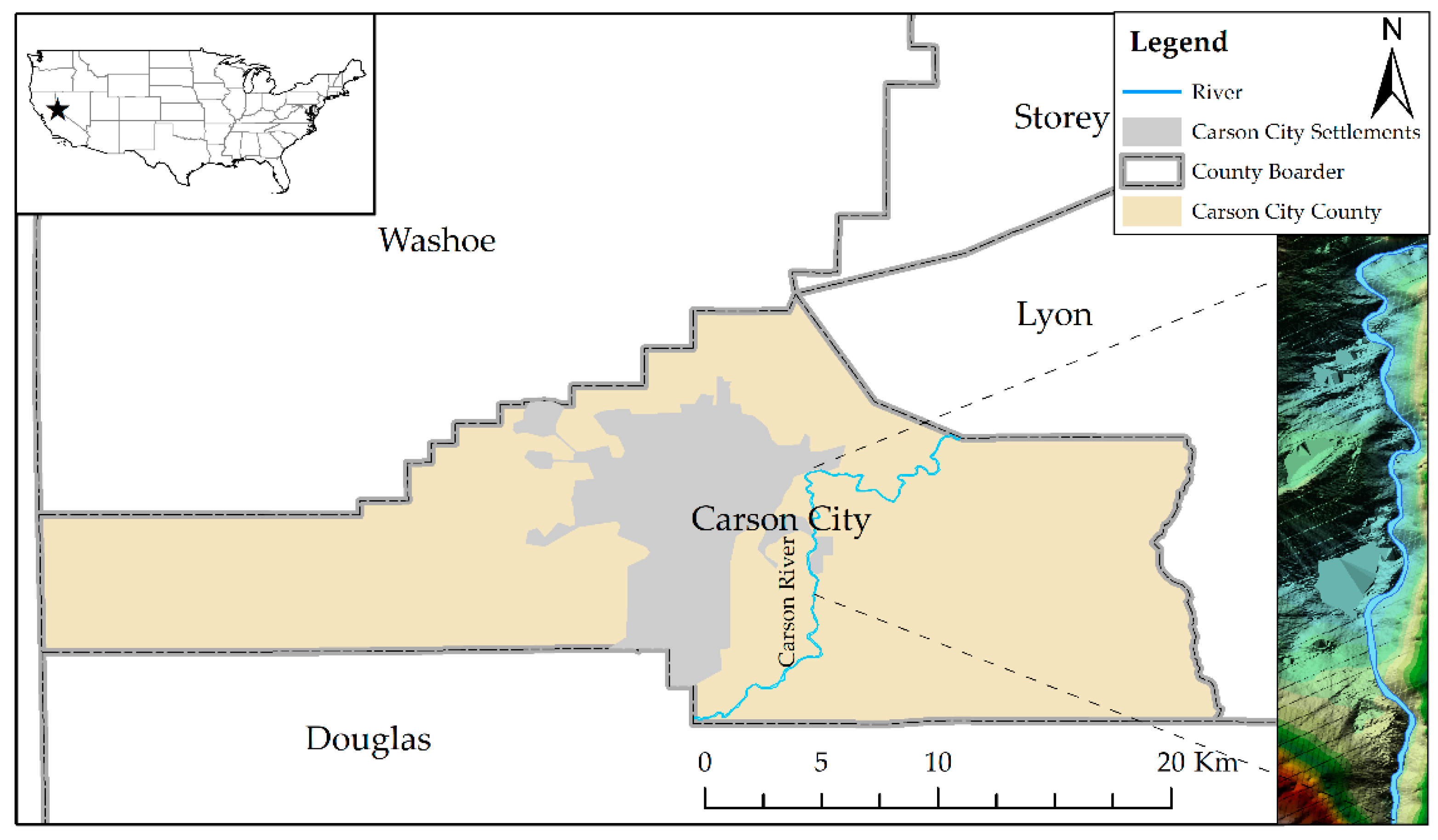
The southwestern United States not only experiences extreme heat but is also vulnerable to extreme flooding due to climate change [41]. Carson City, NV has had, since 1852, a historical record of flood, and is currently experiencing some flooding due to extreme storm events. Carson Valley, which lies 4700–5000 feet above the mean sea level, is the rain shadow of the Sierra Nevada. The highest point of the catchment lies on the Sierra Nevada, and is 11,462 feet above the mean sea level. The climate of the area ranges from semi-arid over the valley plain to humid or super humid over the peaks of the catchment. The catchment receives precipitation mostly as rain at the lower altitude and as snow at the higher altitude. Runoff reaches its yearly peak mainly in May. In this study, the downstream end of Carson River at Carson City is examined for future floods. The selected reach was flooded in 2007, and is susceptible to similar events in the future. The spatial location of the Carson River reach at Carson City selected for the current study is shown in Figure 1. Figure 1 also shows the digital elevation map (DEM) that represents the altitude along the river reach that was considered for hydraulic modeling.
1.2. Data
The latest daily average runoff from 31 AOGCMs participating in the CMIP5 was used to analyze the change in the extreme runoff for Carson River. These CMIP5-AOGCMs have produced the Bias-Corrected Spatially Downscaled (BCSD) streamflow for different streams in the United States from 1950 to 2099. The data produced by these AOGCMs were routed over a historic period of 1950 to 1999. Thus, in this study, the same period of 1950–1999 is considered to be the historic period. The farthest 50-year period i.e., 2050–2099, is considered to be the future period. The VIC-enforced streamflow for 195 different locations is available, among which 152 locations are co-located with the United States Geological Survey (USGS)’s Hydroclimatic Data Network (HCDN), and 43 locations are co-located with West Wide Climate Risk Assessment spatially downscaled locations. Streamflow data for East Fork Carson River near Gardnerville from total 97 projections that were derived through 31 models and four RCPs were used to estimate the change in streamflow due to climate change. The location of the streamflow is at Latitude 38.844° N and Longitude 119.702° W, which is co-located with the ’East Fork Carson River near Gardnerville’ HCDN station (station ID 0071). The projections were used for the future streamflow analysis, while the HCDN station was used for the historic record. The details of the climate model and the relevant institutions are summarized in Table 1.
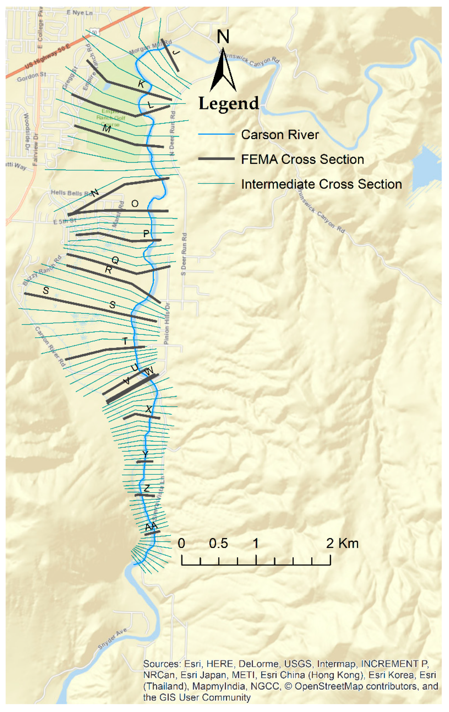
The DEM required for the river terrain was obtained from the USGS National Map viewer. Models using fine-resolution DEM products are more stable and accurate as compared to models that use DEM products of a coarser resolution. Additionally, it is recommended to adopt Light Detecting and Ranging using Remote-Sensing-based products to model a riverine system of higher depths. Due to the limitations of data availability in the study area, the current study utilizes a 1/3 arc-second DEM product for producing the river profile and cross-sections. The river cross-section locations were considered at and in between the Federal Emergency Management Agency (FEMA)’s adopted cross-sections for a comparison purpose. The levee and other existing structures were not adopted in the prepared model as the details of the structures are not readily available. Manning’s roughness values were adopted from the Flood Insurance Study (FIS) for the area [42]. Figure 2 represents the Hydrologic Engineering Center’s River Analysis System (HEC-RAS) geometric model with the river sections. Eighteen of these cross-sections match with the cross-sections in the FEMA-developed flood map.
2. Method
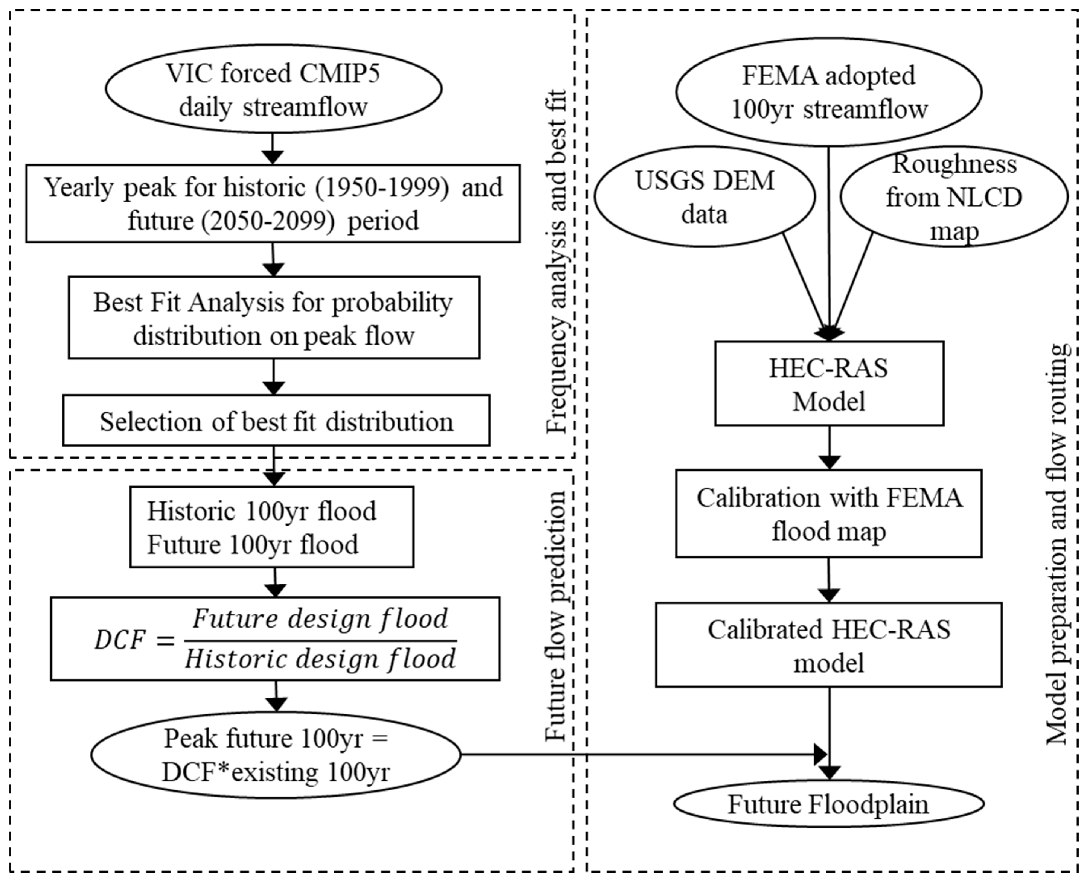
The method section is subdivided into three subsections: (i) Frequency analysis and best fit, (ii) Future flow prediction, and (iii) flow routing.
(i) Frequency analysis and best fit: The streamflow projections, along with the nearby real gauge station, were analyzed with a frequency distribution to find the best-fit frequency distribution for the study area. From the 97 streamflow projections for the historic and future periods, a total of 194 projection datasets, each containing 50 years of yearly peak flow, were prepared. These datasets, along with one Carson River gauge dataset, for a total of 195 datasets, were fitted with 27 different distribution methods to obtain the best-fit distribution. The 27 different distributions that were applied to the datasets are listed in Table 2. The data were tested for goodness of fit with Kolmogorov–Smirnov and Pearson Chi-square tests. The tests were implemented over the 195 datasets for the historic and future periods of the model and the historic gauge data. Each best-fit test returns a significance level as an attained value, which is represented as αattained [43]. The significant level for the Pearson Chi-square test and the Kolmogorov–Smirnov test is given, respectively, by
where, m is the degree of freedom, k is the class interval, r is the number of parameters of the distribution, and q is the computed Pearson parameter, which is given by
where n is the size of the sample.
These analyses were performed utilizing the statistical Hydrognomon software developed by the National Technical University of Athens [43]. Hydrognomon is a robust tool for performing different time-series analyses: regularization of data, interpolation, regression, fitting a distribution function to a time series, statistical predictions, and homogeneity testing. This tool can handle time-series data at different time scales: daily, monthly, and annual. The current study only uses the capabilities of the Hydrognomon tool to fit a distribution function to a hydrologic time series. Hydrognomon includes 27 different functions that were utilized in the current study to fit the historical records with the help of the Pearson Chi-square and Kolmogorov–Smirnov tests. Hydrognomon utilizes the Monte-Carlo algorithm to determine the confidence interval of any fitted distribution function. The best-fit distribution based on the Hydrognomon tool was selected to generate the future streamflow. All 27 distribution functions included in the Hydrognomon tool are summarized in Table 2.
(ii) Future flow prediction: Based on the best-fitted distribution method, 100-year flood (the design flood) was calculated for the historic and projected streamflow datasets. The Delta Change Factor (DCF) was used to calculate the future flow at the stream station. The future flow that was estimated using the FEMA and delta change methods depicts a flood under a stationary condition and a flood under climate change conditions in the future, respectively. Among the range of delta change factor future flows, the peak one was selected to represent the maximum increase in the future design flood’s condition. In this study, it was assumed that the ratio of the downstream peak flow to the upstream peak flow remains same in the future.
(iii) Flow routing: A HEC-RAS model was prepared from the available DEM model. Eighteen cross-sections from the Flood Insurance Rate Map (FIRM) and 58 intermediate cross-sections were prepared for the HEC-RAS model using ArcGIS (Version 10.4, Environmental Systems Research Institute (Esri), Redlands, CA, USA). A total of 76 cross-sections were assigned using the FIS-suggested Manning’s roughness coefficient. The existing 100-year return period’s flow (the design flow) was routed to the prepared model and compared with the existing FIRM map. Finally, the prepared model was routed to the future peak flood, and the hydraulic parameters were compared with the existing design condition of the FEMA map. The aforementioned steps involved in flow routing and flood plain delineation is summarized as the flowchart in Figure 3.
3. Results
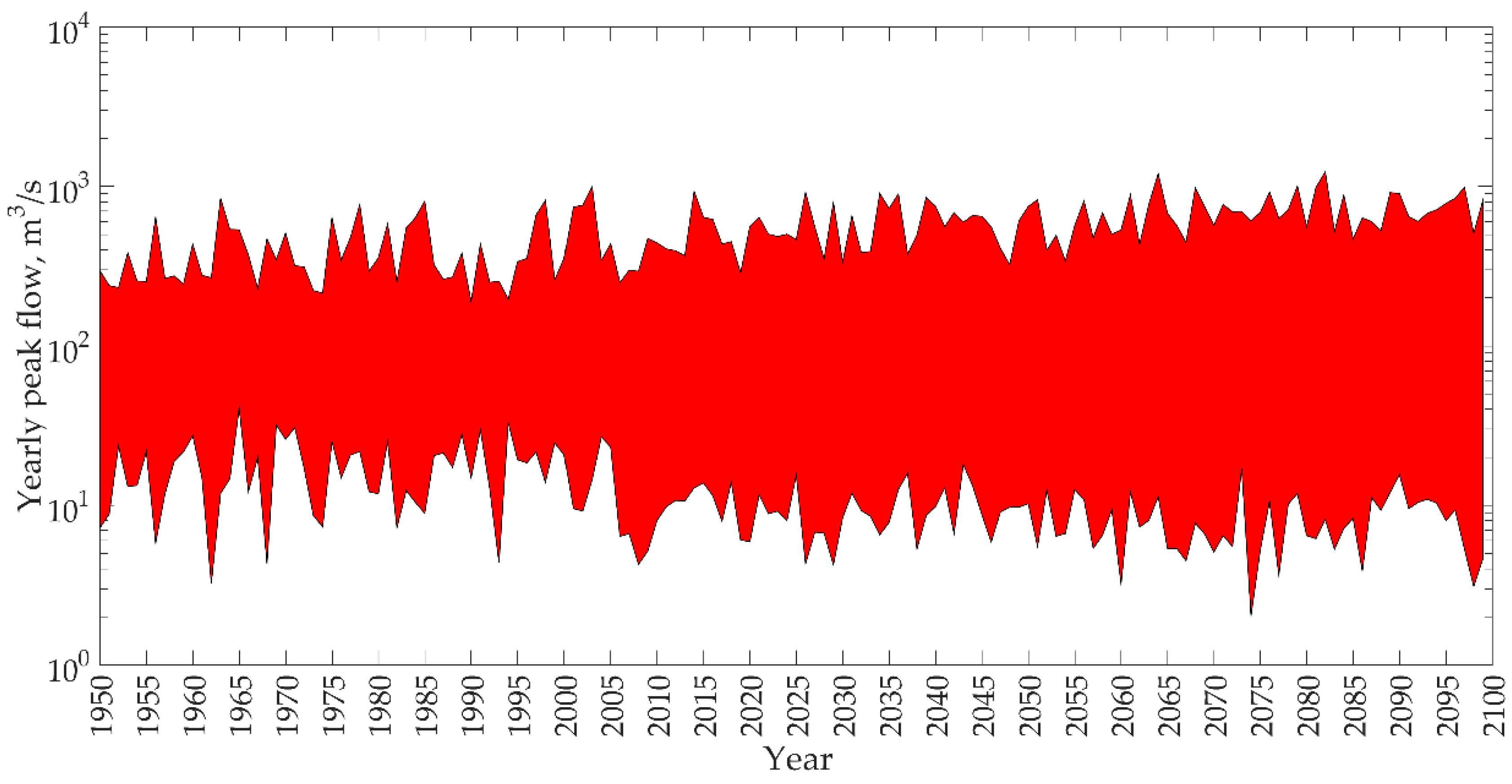
The daily streamflow series that was derived from the climate model projections shows a clear trend of an increasing future peak streamflow in Carson River and, at the same time, a decreasing yearly peak minimum, as shown in Figure 4. This signifies the occurrence of both more intense high flows and low flows as shown by the spread time series in Figure 4, which increases along the positive abscissa. The maximum and minimum yearly flow plotted in Figure 4 were obtained from 97 streamflow projections of 31 models and four RCPs. In this study, only the probable maximum flow was analyzed, as the study area is subject to a greater flood risk as a result of the high flows as compared to the low flows.
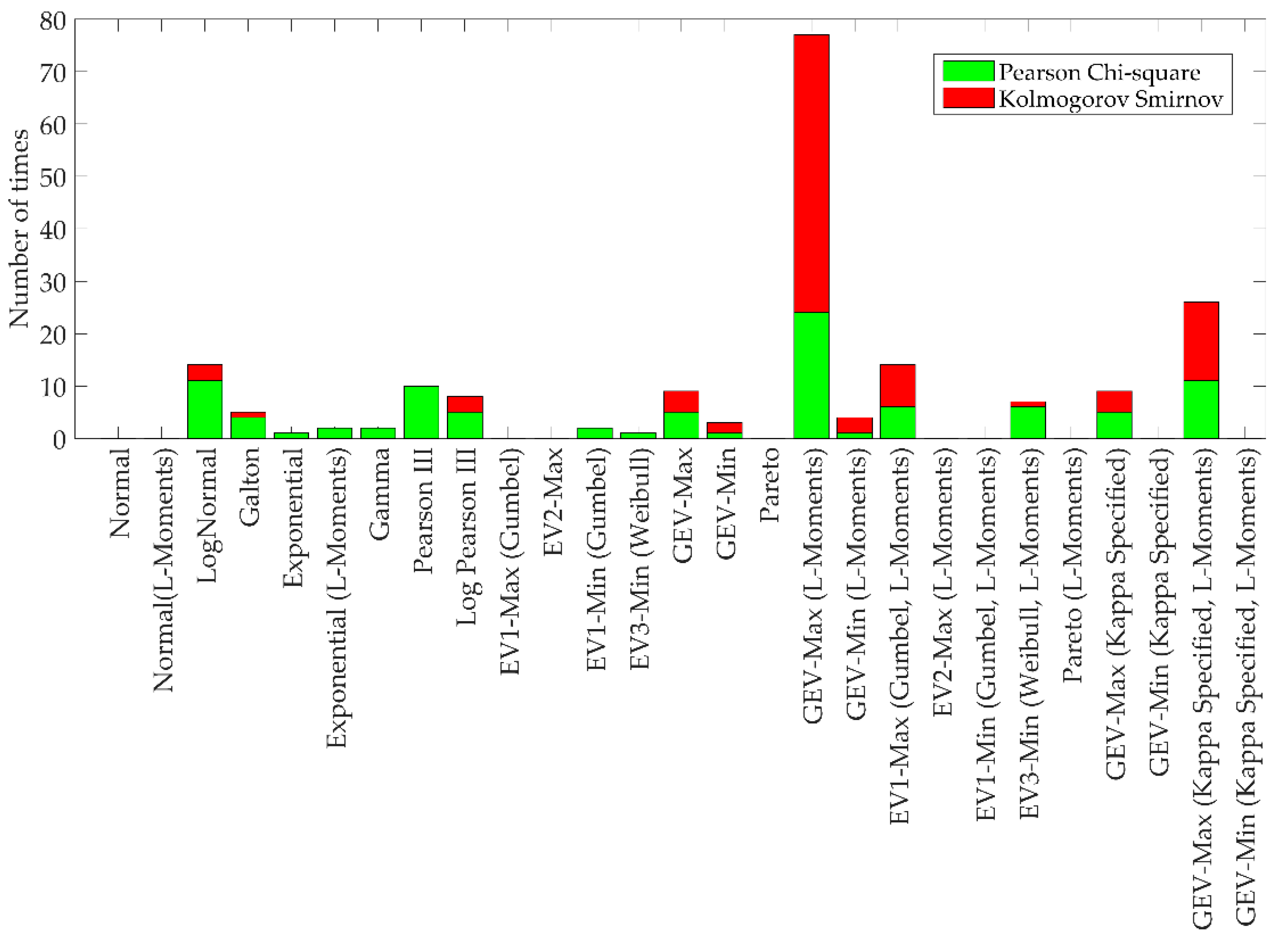
Yearly maximum streamflow data from the 97 climate projections from 1950 to 2099 were selected and analyzed using Pearson Chi-square and Kolmogorov–Smirnov tests. The best fit from both models is presented in Figure 5. The bars in Figure 5 represent the number of projections that was best-fitted with a specific distribution method from the two different tests. From Figure 5, GEV-Max (L-Moments) was selected as the best-fit distribution from the Pearson Chi-square and Kolmogorov–Smirnov tests, with a count of 24 and 53, respectively, out of 97 total projections. Thus, GEV-Max (L-moments) was found to be the best distribution method and selected to analyze future floods in the study area.
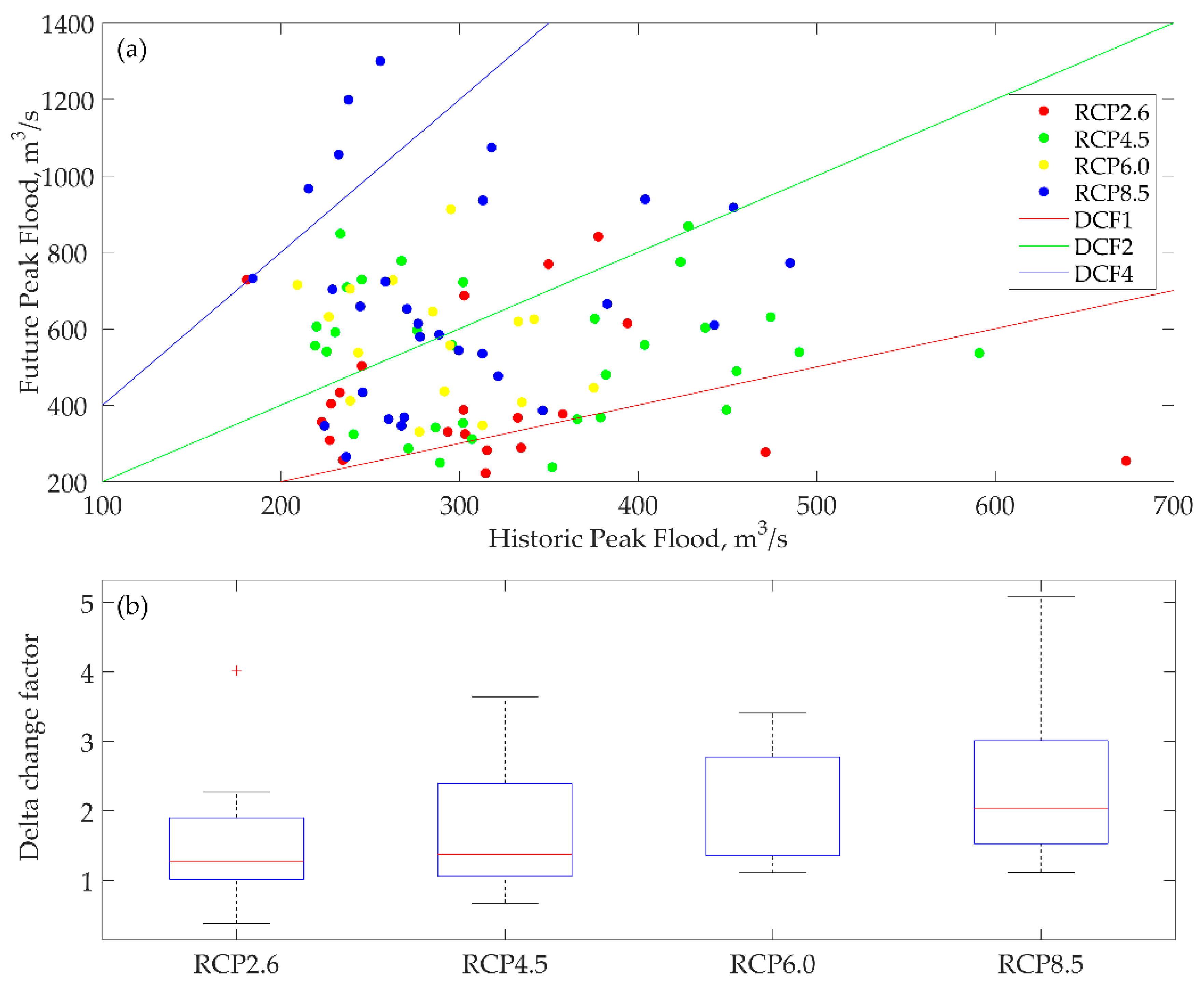
The best-fit distribution method, GEV-Max (L-Moments), was used to calculate the peak flow over 100 years (the design flow) for the historic and future period. The selected distribution method was used to calculate the Delta Change Factor. The delta change factor is the ratio of the future to the historic design flow. It was calculated from each climate model, and the values of the delta change factor are summarized in Figure 6a. The inclined lines DCF1, DCF2, and DCF4 represent the delta change factors 1, 2, and 4, respectively, which represent that the future design flood would be the same, two times, and four times the historic period, respectively. In the figure, each emission scenario projection is represented with a different color so that they can be easily distinguished. Figure 6b represents the boxplot of the DCFs corresponding to each RCP. The red-colored horizontal lines in the boxplots represent the median and horizontal edges of the boxes, which represent the 25th and 75th percentiles, respectively, of the DCFs corresponding to each RCP. Similarly, the whiskers in the boxplots represent the 5th and 95th percentiles, and the red data point corresponding to RCP2.6 boxplot is the outlier. From Figure 6a, RCP2.6 has the lowest delta change factor, and RCP8.5 has the highest delta change factor. Figure 6b represents that, with an increase in greenhouse gases, the future extremes of streamflow are expected to increase. Although the two lower RCPs have only a few models with a delta change factor of less than one, the higher RCPs have a DCF that is greater than one. For the flood mapping, the maximum delta change factor of 5.086, which was obtained from the CNRM-CM5 model with RCP8.5, is considered.
Table 3 shows a hydrological summary of USGS gauge site 1031000 in Carson City, for which a flood analysis has been carried out that developed estimates of flood chance for different return periods. For this study’s purpose, only the 1% chance and the 0.2% chance of an annual occurrence, i.e., the 100-year and 500-year return periods, were used. FEMA has developed estimates of the 100-year and 500-year return period flows for the selected study area. A FIRM map with the panel numbers 3200010227E, 3200010112E, and 3200010114F covers the study area.
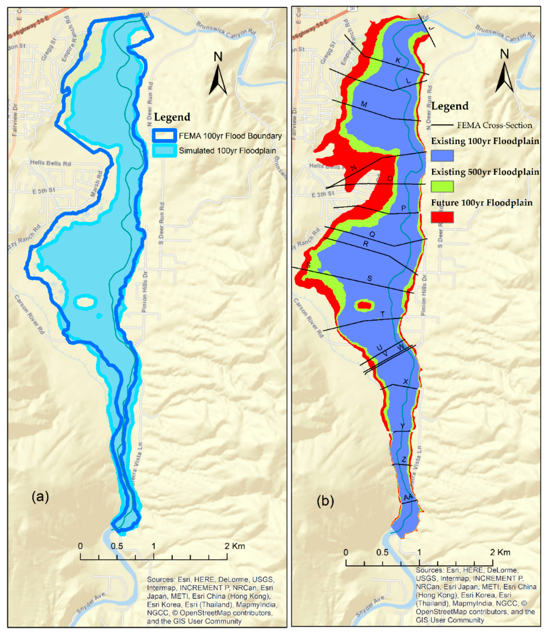
The calibration of the HEC-RAS two-dimensional (2D) model was performed with 100 years of historic streamflow data that was obtained from the gauge site. The calibration was done by comparing the HEC-RAS-generated floodplain map for the past 100 years with FEMA’s 100-year flood boundary estimation. A perfect model would result in the same HEC-RAS-generated floodplain map as compared to the FEMA 100-year flood boundary estimation. This result is shown in Figure 7a. Some discrepancy may be attributed to the errors associated with the Manning’s roughness coefficient of the reach, which is a function of how a river meanders and channel bed roughness. The robustness of the HEC-RAS model was established with its conformity to the simulated water surface elevation and the observed gauge height at USGS gage station 10311400, which is located downstream of the selected river reach. The Nash–Sutcliffe efficiency coefficient (NSE), the correlation coefficient (R2), and the percent bias (P-Bias) were computed with the simulated water surface elevation resulting from the observed streamflow that was recorded at USGS gauge station 10311400 corresponding to the observed gauge height. Based on the observed and simulated data, the NSE, R2, and P-Bias were evaluated as 0.79, 0.98, and −0.008, respectively. These statistical parameters demonstrate the robustness of the calibrated HEC-RAS model, and the water surface elevation predicted by the model can be utilized to generate a future floodplain map with the estimated future streamflow.
The delta change factor that was calculated for the study was used to calculate the future design flood (the flood flow over 100 years). The future design flood flow comes to be 5185 m3/s, which is more than the current 500-year flood flow. Thus, the climate-generated future design flood flow may be greater than the recent 500-year flood flow. The developed HEC-RAS model routed for the three different flood flows, that is, the existing 100-year, the existing 500-year, and the future 100-year flows, a discharge of 1020 m3/s, 2560 m3/s, and 5185 m3/s, respectively. The flood area developed using HEC-RAS and ArcGIS is presented in Figure 7b. The floodplain for the present design flood flow, the present 500-year flood flow, and the future design flood flow was plotted. The area covered by these three conditions is 3,915,290 m2, 4,762,168 m2, and 5,947,893 m2, respectively, while the FEMA 100-year flood flow covers 4,882,183 m2. The floodplain for each of these three conditions was compared, and it was observed that the extreme future 100-year floodplain could cover more than 1.5 times the area covered by the present 100-year floodplain.
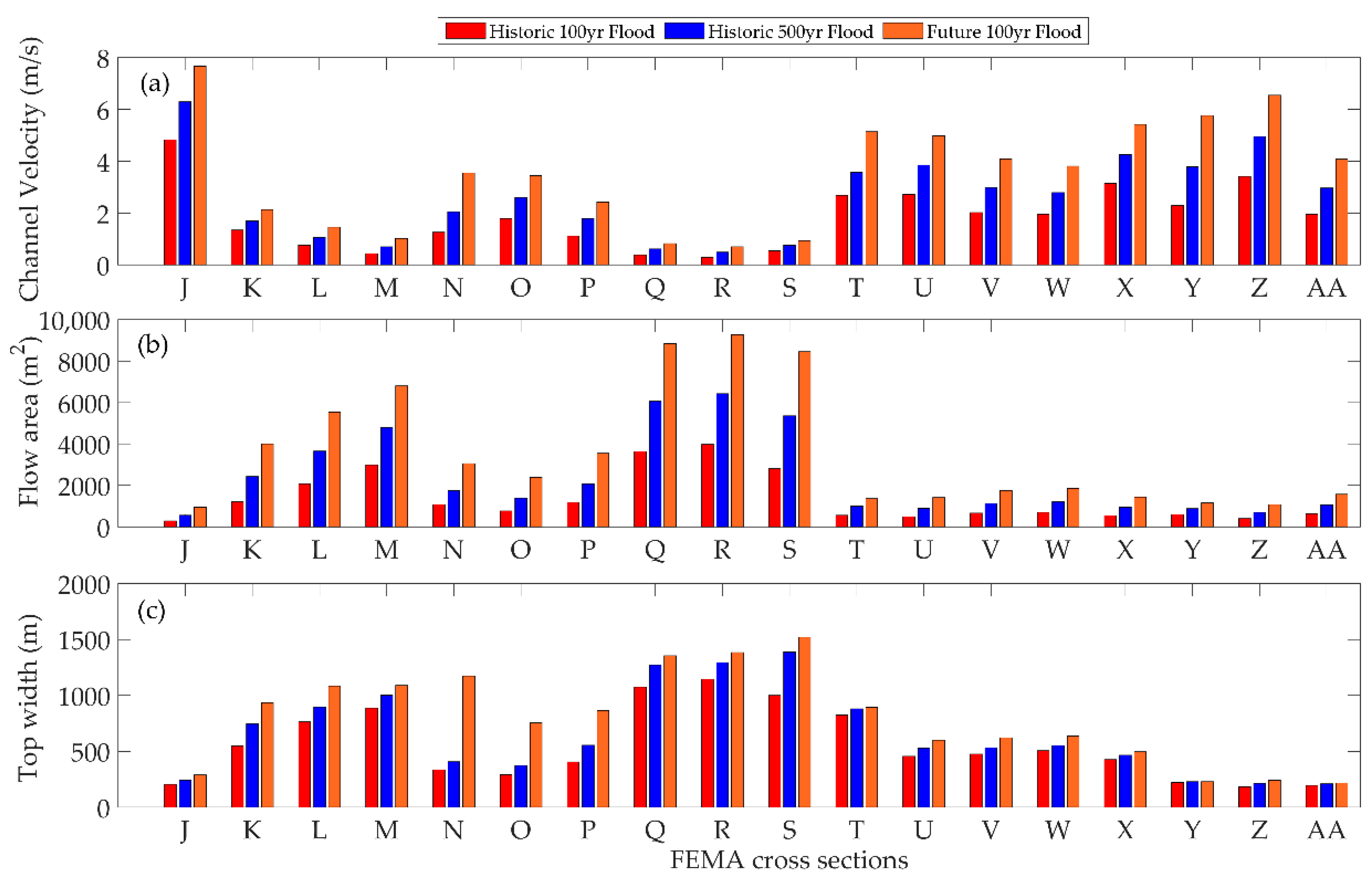
Further, the channel velocity, flow area, and top width were compared between the historic 100-year, the historic 500-year, and the future 100-year floods. The FIRM map has 18 cross-sections within the reach length. Hydraulic parameters, such as channel velocity, flow area, and top width, were compared within this reach length and the FIRM map cross sections, and are presented in Figure 8. The calibration of the HEC-RAS model can also be verified from Figure 7a, which shows a similar floodplain for 100-year event as compared to the 100-year event from the FIRM map. The generated floodplain maps shows that there will be more flooding on the left bank of the river than the right due to its topography. In addition, the city nearby the river might be affected due to this change in future flow. The low-lying agricultural land on the Carson floodplain will be vulnerable to flooding events in the future, as our results suggest that these events will be more intense than in the past.
Channel velocity, flow area, and top width are the key hydraulic parameters of floods, and were compared under different flow conditions. The future 100-year flood has the highest channel velocity (around 8 m/s). The channel flow area will more than double at most of the cross-sections, and there will be a significant increase in the top width along sections N, O, and P.
4. Discussion
Floodplain management should reduce flood damage in the future with efficient mitigation measures at minimal expense. A flood protection decision can endure for more than a century; thus, it is worth considering long-term changes in environmental conditions. A decision on floodplain management would likely affect the long-term performance of infrastructure [44]. As human beings have evolved, societies have started to inhabit places close to freshwater to ensure water for drinking and agricultural and livestock use. Major civilizations of the past settled very close to rivers with an adequate supply of fresh water. More than half of the total global population resides within 3 km from freshwater bodies, mostly near a river [45]. This population is more vulnerable to changes in streamflow in the future. In this study, such a case is analyzed using CMIP5 hydrologic projections. The CMIP5 data helped to predict the nature of future streamflow without assuming stationarity in the hydro-climatic data. Further, CMIP5 models consider different carbon emission scenarios, allowing us to comprehend a wide range of future streamflow conditions.
As different probability distributions result in different flood frequencies, selecting an appropriate flood distribution method is crucial in flood frequency analysis. To select the best-fit distribution, two different tests—the Pearson Chi-Square and the Kolmogorov–Smirnov—were implemented. The selected distribution was used to predict the design flood for present and future datasets of climate projections. Further, the performance of different distribution methods varies spatially. Thus, one distribution that performs well for a given dataset of an area may not represent another distribution. Thus, it is always recommended to analyze the results that are obtained with different distributions, and the best distribution should be selected with a different approach. It is good to test a variety of statistical distributions; however, at the same time, it is impractical to test all of the possible distributions. In the current study, the selected distributions were based on a previous study that was pertinent to the climatic conditions of the selected study region. Testing other distributions over a wide variety of watersheds is recommended for future studies. Both the Pearson Chi-Square test and the Kolmogorov–Smirnov test showed that GEV-max (L-moment) was the best distribution. Previous studies suggest that GEV is to likely to fit the streamflow across semi-arid regions, which was also established in the current findings [32,33,34,38,39].
From the 97 total models/selections, the Pearson Chi-square test and the Kolmogorov–Smirnov test selected GEV-max (L-moment) 24 and 53 times, respectively. GEV-max (L-moment) was then used to calculate the design flow for the present and future periods. Among the 97 models, 86 models had a DCF greater than one, suggesting that the design flow for the future period should be more than that for the present period. This suggests that there is a higher possibility that the design flow on the river would be higher in the future. Among the 97 models, 39 (more than 40% of the models) indicated that the design flow in the future will be more than 2 times the present design flow. The DCF results also show that the higher the emission or RCP, the higher the delta change factor will be, which represents an increase in the design flow in the future. The delta change method was adopted to predict the flow of future floods, which was routed on a HEC-RAS one-dimensional (1D) model to compare the floodplain and hydraulic parameters.
The maximum increase in future design flow resulted from the CNRM-CM5 model with the RCP8.5 scenario and the maximum DCF. The CNRM-CM5 model with RCP8.5 scenario was also considered for the flood mapping of the Carson River near Carson City, Nevada as it would represent the most extreme flooding scenario. The model indicates that a 5.086-fold increase in the design flow of the river will occur. This suggests that the future 100-year flood flow will be more than that of the current 500-year flow, while the future 100-year flood flow will be more than 1.5 times the current 100-year flood flow. The floodplain map showed an increase in the extent of the flooding in the future as compared to that of current flooding events. Most of the GCMs suggested an increase in the future design flow when compared to present conditions, which can be attributed to the nonstationary nature of the climate. Further, the floodplain variability in the future may also be affected by other factors, such as a change in land use [46]. An increase in the streamflow in a semi-arid region as a result of climate change has also been documented by previous studies. For example, an increase in streamflow has been projected for the city of Las Vegas [47], and a positive streamflow trend has been documented in the Colorado River basin [48].
The population of Carson City is settled on the left bank of the Carson River. The topography of the river shows that the river has more floodplain on left side than on the right side. The floodplain contains fertile agricultural land that is crucial, as Carson City lies in the desert of Nevada. Due to the predicted increase in the design flood flow in the future, more area than expected might be flooded. Future flooding will not only affect the agricultural supply but also people residing near the river. Thus, a proper analysis of future streamflow will help to minimize the flood risk. The current study’s evaluation of the best-fit distribution, and use of a climate distribution, to evaluate the future streamflow frequency suggested that the streamflow data has a nonstationary nature as a result of climate variability and change. Thus, future design streamflow may not be same as the current design streamflow. This should be considered by planners and engineers when planning and building new hydraulic structures to minimize the flood risks associated with the changing climate.
5. Conclusions
The risk of hydrologic extremes as a result of the changing climate is one of the main global challenges of the 21st century. This risk has been increasing in recent years, as limited effort has been made to curb the emission of greenhouse gases. Most governmental agencies apply stationary approaches to flood management. Due to this, the effect of climate change cannot be incorporated into flood flow predictions. Thus, this study suggests the possible approach of applying a nonstationary approach to future streamflow prediction in those regions vulnerable to flooding events. As most flood management structures are constructed for a lifespan of several decades to more than a century, forecasting streamflow while considering the effects of climate change can contribute to the optimization of hydraulic structures. Hence, this study’s contribution is to present guidelines to planners, designers, engineers, and policy-makers for incorporating climate change into flood risk management. The current study was focused on the Carson River at Carson City at a regional scale; so, the results may not be similar to those obtained from other watersheds, whilst the proposed algorithm can be utilized elsewhere.
The key findings of the current study are as follows:
- The best-fit distribution was evaluated utilizing both Pearson Chi-square and Kolmogorov Smirnov tests for the considered study area.
- A majority of the climate models indicated an increase in the future streamflow in the study region, while 40 percent of the models suggested that the future 100-year streamflow would be more than 2 times the present 100-year streamflow in the selected study area.
- A higher increase in the future 100-year streamflow was observed for a higher RCP, suggesting that the streamflow in the study region will increase as carbon emissions increase.
- A majority of climate models depicted DCFs higher than 1, suggesting that the streamflow in the Carson River exhibits nonstationary behavior and that the future streamflow is likely to exceed that of the past.
- The CNRM-CM5 model with the RCP8.5 scenario showed the maximum increase in future runoff for the Carson River.
- The future flow, depth of flow, and inundation comparison gave an explicit image of the extent of future flooding due to climate change for the Carson River at Carson City.
- The extent of flooding of the future 100-year streamflow for the Carson River at Carson City was evaluated to be higher than that of the past 500-year streamflow, highlighting the likelihood of an increase in the extent of future flooding.
To summarize, hydraulic structures are conventionally designed for different return periods assuming the stationarity in the streamflow. The current research highlights the utilization of climate information for evaluating the future streamflow in different recurrence intervals. This future streamflow is then used to evaluate future floodplain maps and design the streamflow. We also recommend testing the application of other statistical distributions to a variety of watersheds with a higher resolution dataset in the future to extend the current study.
Author Contributions
A.K. and S.A. designed the research idea and the results are prepared by N.N. and B.T. All the authors analyzed the results and wrote the paper together.
Funding
This research received no external funding.
Acknowledgements
The authors would like to thank three anonymous reviewers for providing valuable comments. We acknowledge the Program for Climate Model Diagnosis and Intercomparison (PCMDI) and the World Climate Research Programme (WCRP) Working Group on Coupled Modelling (WGCM) for their role in making available the WCRP CMIP5 multi-model dataset. Support for this dataset is provided by the Office of Science, U.S. Department of Energy. The authors would like to acknowledge the Office of the Vice Chancellor for Research at Southern Illinois University, Carbondale for providing the research support. Thanks to Ankit Kumar from the Indian Institute of Technology, Mumbai, India for his valuable suggestions during the preparation of this manuscript.
Conflicts of Interest
The authors declare no conflict of interest.
Abbreviations
| AOGCM | Atmosphere-Ocean Coupled General Circulation Model |
| BCSD | Bias Corrected Statistically Downscaled |
| CMIP | Coupled Model Intercomparison Project |
| DCF | Delta Change Factor |
| DEM | Digital Elevation Model |
| FEMA | Federal Emergency Management Agency |
| FIRM | Flood Insurance Rate Map |
| FIS | Flood Insurance Study |
| GCM | General Circulation Model |
| GEV | Generalized Extreme Value |
| RCP | Representative Concentration Pathways |
| VIC | Variable Infiltration Capacity |
| WCRP | World Climate Research Programme |
References
- IPCC. Summary for Policymakers. In Climate Change 2013: The Physical Science Basis. Contribution of Working Group I to the Fifth Assessment Report of the Intergovernmental Panel on Climate Change; Stocker, T.F., Qin, D., Plattner, G.-K., Tignor, M., Allen, S.K., Boschung, J., Nauels, A., Xia, Y., Bex, V., Midgley, P.M., Eds.; Cambridge University Press: Cambridge, UK, 2013. [Google Scholar]
- Dlamini, N.S.; Kamal, M.R.; Soom, M.A.B.M.; Mohd, M.S.F.; Abdullah, A.F.B.; Hin, L.S. Modeling potential impacts of climate change on streamflow using projections of the 5th assessment report for the Bernam River basin, Malaysia. Water 2017, 9, 226. [Google Scholar] [CrossRef]
- Hirabayashi, Y.; Kanae, S.; Emori, S.; Oki, T.; Kimoto, M. Global projections of changing risks of floods and droughts in a changing climate. Hydrolog. Sci. J. 2008, 53, 754–772. [Google Scholar] [CrossRef] [Green Version]
- Kefi, M.; Mishra, B.K.; Kumar, P.; Masago, Y.; Fukushi, K. Assessment of tangible direct flood damage using a spatial analysis approach under the effects of climate change: Case study in an urban watershed in Hanoi, Vietnam. ISPRS Int. J Geo-Inf. 2018, 7, 29. [Google Scholar] [CrossRef]
- Nohara, D.; Kitoh, A.; Hosaka, M.; Oki, T. Impact of climate change on river discharge projected by multimodel ensemble. J. Hydrometeorol. 2006, 7, 1076–1089. [Google Scholar] [CrossRef]
- Rafiei Emam, A.; Mishra, B.K.; Kumar, P.; Masago, Y.; Fukushi, K. Impact assessment of climate and land-use changes on flooding behavior in the upper Ciliwung River, Jakarta, Indonesia. Water 2016, 8, 559. [Google Scholar] [CrossRef]
- Yerramilli, S. Potential impact of climate changes on the inundation risk levels in a dam break scenario. ISPRS Int. J. Geo-Inf. 2013, 2, 110–134. [Google Scholar] [CrossRef]
- Dankers, R.; Feyen, L. Flood hazard in Europe in an ensemble of regional climate scenarios. J. Geophys. Res. Atmos. 2009, 114. [Google Scholar] [CrossRef] [Green Version]
- Davie, J.C.; Falloon, P.D.; Kahana, R.; Dankers, R.; Betts, R.; Portmann, F.T.; Wisser, D.; Clark, D.B.; Ito, A.; Masaki, Y. Comparing projections of future changes in runoff from hydrological and biome models in ISI–MIP. Earth Syst. Dyn. 2013, 4, 359–374. [Google Scholar] [CrossRef]
- Hirabayashi, Y.; Mahendran, R.; Koirala, S.; Konoshima, L.; Yamazaki, D.; Watanabe, S.; Kim, H.; Kanae, S. Global flood risk under climate change. Nat. Clim. Chang. 2013, 3, 816–821. [Google Scholar] [CrossRef]
- Koirala, S.; Hirabayashi, Y.; Mahendran, R.; Kanae, S. Global assessment of agreement among streamflow projections using CMIP5 model outputs. Environ. Res. Lett. 2014, 9. [Google Scholar] [CrossRef]
- NCEI (National Centers for Environmental Information). U.S. Billion-Dollar Weather and Climate Disasters, 2018. NCEI Web Site. Available online: https://www.ncdc.noaa.gov/billions/ (accessed on 3 October 2018).
- Wobus, C.; Gutmann, E.; Jones, R.; Rissing, M.; Mizukami, N.; Lorie, M.; Mahoney, H.; Wood, A.W.; Mills, D.; Martinich, J. Modeled changes in 100 year flood risk and asset damages within mapped floodplains of the contiguous United States. Nat. Hazards Earth Syst. Sci. Discuss. 2017. [Google Scholar] [CrossRef]
- Papalexiou, S.M.; AghaKouchak, A.; Trenberth, K.E.; Foufoula-Georgiou, E. Global, regional, and megacity trends in the highest temperature of the year: Diagnostics and evidence for accelerating trends. Earth’s Future 2018, 6, 71–79. [Google Scholar] [CrossRef] [PubMed]
- Van Aalst, M.K. The impacts of climate change on the risk of natural disasters. Disasters 2006, 30, 5–18. [Google Scholar] [CrossRef] [PubMed]
- Lamichhane, N.; Sharma, S. Development of flood warning system and flood inundation mapping using field survey and LiDAR data for the Grand River near the city of Painesville, Ohio. Hydrology 2017, 4, 24. [Google Scholar] [CrossRef]
- Taylor, K.; Stouffer, R.; Meehl, G. A summary of the CMIP5 experiment design. January 2011, 22, 33. [Google Scholar]
- Taylor, K.E.; Stouffer, R.J.; Meehl, G.A. An overview of CMIP5 and the experiment design. Bull. Am. Meteorol. Soc. 2012, 93, 485–498. [Google Scholar] [CrossRef]
- Wood, A.W.; Leung, L.R.; Sridhar, V.; Lettenmaier, D. Hydrologic implications of dynamical and statistical approaches to downscaling climate model outputs. Clim. Chang. 2004, 62, 189–216. [Google Scholar] [CrossRef]
- Maurer, E.; Wood, A.; Adam, J.; Lettenmaier, D.; Nijssen, B. A long-term hydrologically based dataset of land surface fluxes and states for the conterminous United States. J. Clim. 2002, 15, 3237–3251. [Google Scholar] [CrossRef]
- Hidalgo, H.G.; Dettinger, M.D.; Cayan, D.R. Downscaling with Constructed Analogues: Daily Precipitation and Temperature Fields over the United States. In California Energy Commission PIER Final Project Report; CEC-500-2007-123; California Energy Commission: Sacramento, CA, USA, 2008. [Google Scholar]
- Mote, P.W.; Salathe, E.P. Future climate in the Pacific Northwest. Clim. Chang. 2010, 102, 29–50. [Google Scholar] [CrossRef] [Green Version]
- Fowler, H.J.; Blenkinsop, S.; Tebaldi, C. Linking climate change modelling to impacts studies: Recent advances in downscaling techniques for hydrological modelling. Int. J. Climatol. 2007, 27, 1547–1578. [Google Scholar] [CrossRef]
- Gangopadhyay, S.; Pruitt, T.; Brekke, L. West-Wide Climate Risk Assessments: Bias-Corrected and Spatially Downscaled Surface Water Projections; US Department of the Interior, Bureau of Reclamation, Technical Service Center: Denver, CO, USA, 2011.
- Milly, P.C.; Dunne, K.A.; Vecchia, A.V. Global pattern of trends in streamflow and water availability in a changing climate. Nature 2005, 438, 347–350. [Google Scholar] [CrossRef] [PubMed]
- Liang, X.; Lettenmaier, D.P.; Wood, E.F.; Burges, S.J. A simple hydrologically based model of land surface water and energy fluxes for general circulation models. J. Geophys. Res. Atmos. 1994, 99, 14415–14428. [Google Scholar] [CrossRef]
- Liang, X. Variable Infiltration Capacity (VIC): Macroscale Hydrologic Model, 2002. VIC Documentation Web Site. Available online: http://www.hydro.washington.edu/Lettenmaier/Models/VIC/VIChome.html (accessed on 20 August 2018).
- Liang, X.; Wood, E.F.; Lettenmaier, D.P. Surface soil moisture parameterization of the VIC-2L model: Evaluation and modification. Glob. Planet Chang. 1996, 13, 195–206. [Google Scholar] [CrossRef]
- Nijssen, B.; Lettenmaier, D.P.; Liang, X.; Wetzel, S.W.; Wood, E.F. Streamflow simulation for continental-scale river basins. Water Resour. Res. 1997, 33, 711–724. [Google Scholar] [CrossRef] [Green Version]
- Brekke, L.; Wood, A.; Pruitt, T. Downscaled CMIP3 and CMIP5 Hydrology Projections: Release of Hydrology Projections, Comparison with Preceding Information, and Summary of User Needs; US Department of the Interior Bureau of Reclamation: Denver, CO, USA, 2014.
- Brekke, L.; Thrasher, B.; Maurer, E.; Pruitt, T. Downscaled CMIP3 and CMIP5 Climate Projections: Release of Downscaled CMIP5 Climate Projections, Comparison with Preceding Information, and Summary of User Needs; US Department of the Interior, Bureau of Reclamation, Technical Service Center: Denver, CO, USA, 2013.
- Ahmed, S.; Tsanis, I. Hydrologic and hydraulic impact of climate change on Lake Ontario tributary. Am. J. Water Resour. 2016, 4, 1–15. [Google Scholar]
- Thakali, R.; Kalra, A.; Ahmad, S. Understanding the effects of climate change on urban stormwater infrastructures in the Las Vegas Valley. Hydrology 2016, 3, 34. [Google Scholar] [CrossRef]
- Moglen, G.E.; Vidal, G.E.R. Climate change impact and storm water infrastructure in the Mid-Atlantic region: Design mismatch coming. J. Hydrol. Eng. 2014, 19. [Google Scholar] [CrossRef]
- Zhu, J. Impact of climate change on extreme rainfall across the United States. J. Hydrol. Eng. 2013, 18, 1301–1309. [Google Scholar] [CrossRef]
- Zhu, J.; Stone, M.C.; Forsee, W. Analysis of potential impact of climate change on intensity-duration-frequency (IDF) relationships for six regions in the United States. J. Water Clim. Chang. 2012, 3, 185–196. [Google Scholar] [CrossRef]
- Hailegeorgis, T.T.; Alfredsen, K. Regional flood frequency analysis and prediction in ungauged basins including estimation of major uncertainties for mid-Norway. J. Hydrol. Reg. Stud. 2017, 9, 104–126. [Google Scholar] [CrossRef]
- Farquharson, F.A.K.; Meigh, J.R.; Sutcliffe, J.V. Regional flood frequency analysis in arid and semi-arid areas. J. Hydrol. 1992, 138, 487–501. [Google Scholar] [CrossRef]
- Simmers, I. Hydrological Processes and Water Resources Management. In Understanding Water in a Dry Environment; CRC Press: Boca Raton, FA, USA, 2005; pp. 17–30. [Google Scholar]
- Canfield, R.V.; Olsen, D.; Hawkins, R.; Chen, T. Use of Extreme Value Theory in Estimating Flood Peaks from Mixed Populations; Utah State University: Logan, UT, USA, 1980; p. 577. [Google Scholar]
- Jardine, A.; Merideth, R.; Black, M.; LeRoy, S. Assessment of Climate Change in the Southwest United States: A Report Prepared for the National Climate Assessment; Island press: Washington, DC, USA, 2013. [Google Scholar]
- FEMA (Federal Emergency Management Agency). Flood Insurance Study; Number 320001V000C, Version Number 2.3.3.0; FEMA: Washington, DC, USA, 2016.
- Kozanis, S.; Christofides, A.; Mamassis, N.; Efstratiadis, A.; Koutsoyiannis, D. Hydrognomon-Open Source Software for the Analysis of Hydrological Data. Geophys. Res. Abstr. 2010, 12, 12419. [Google Scholar]
- Zhu, T.; Lund, J.R.; Jenkins, M.W.; Marques, G.F.; Ritzema, R.S. Climate change, urbanization, and optimal long-term floodplain protection. Water Resour. Res. 2007, 43. [Google Scholar] [CrossRef] [Green Version]
- Kummu, M.; De Moel, H.; Ward, P.J.; Varis, O. How close do we live to water? A global analysis of population distance to freshwater bodies. PloS ONE 2011, 6. [Google Scholar] [CrossRef] [PubMed]
- Jobe, A.; Kalra, A.; Ibendahl, E. Conservation reserve program effects on floodplain land cover management. J. Environ. Manag. 2018, 214, 305–314. [Google Scholar] [CrossRef] [PubMed]
- Forsee, W.J.; Ahmad, S. Evaluating urban storm-water infrastructure design in response to projected climate change. J. Hydrol. Eng. 2011, 16, 865–873. [Google Scholar] [CrossRef]
- Kalra, A.; Sagarika, S.; Pathak, P.; Ahmad, S. Hydro-climatological changes in the Colorado River basin over a century. Hydrol. Sci. J. 2017, 62, 2280–2296. [Google Scholar] [CrossRef]
Figure 1.
Carson River flowing through Carson City in Nevada.

Figure 2.
Carson River with the intermediate cross sections and the Federal Emergency Management Agency (FEMA) cross-sections. Sources: Esri, HERE, DeLorme, USGS, Intermap, INCREMENT P, NRCan, Esri Japan, METI, Esri China (Hong Kong), Esri Korea, Esri (Thailand), MapmyIndia, NGCC, ® OpenStreetMap contributors, and the GIS User Community.

Figure 3.
The best fit analysis, future design flow prediction, and future design flow routing using HEC-RAS. VIC, Variable Infiltration Capacity; DCF, Delta Change Factor; DEM, digital elevation mode; HEC-RAS, Hydrologic Engineering Center’s River Analysis System; NLCD, National Land Cover Data.
Figure 3.
The best fit analysis, future design flow prediction, and future design flow routing using HEC-RAS. VIC, Variable Infiltration Capacity; DCF, Delta Change Factor; DEM, digital elevation mode; HEC-RAS, Hydrologic Engineering Center’s River Analysis System; NLCD, National Land Cover Data.

Figure 4.
The spread of the band of yearly peak flow from the 97 climate projections, indicating the variability in the future streamflow.
Figure 4.
The spread of the band of yearly peak flow from the 97 climate projections, indicating the variability in the future streamflow.

Figure 5.
The best fit analysis for the 27 different distributions using Pearson Chi-square and Kolmogorov–Smirnov tests.
Figure 5.
The best fit analysis for the 27 different distributions using Pearson Chi-square and Kolmogorov–Smirnov tests.

Figure 6.
A comparison of the delta change factors from the 97 climate projections. (a) Historic versus future design flow (the peak flow over 100 years), (b) box plots comparing the delta change factor for different RCPs.
Figure 6.
A comparison of the delta change factors from the 97 climate projections. (a) Historic versus future design flow (the peak flow over 100 years), (b) box plots comparing the delta change factor for different RCPs.

Figure 7.
(a) A comparison of the Flood Insurance Rate Map (FIRM)’s 100-year flood area versus the baseline scenario (the 100-year flood area obtained from the HEC-RAS model). (b) The three layers of flood area for the 100-year historic, 500-year historic, and 100-year future floodplains (from a smaller to a larger area, respectively). Sources: Esri, HERE, DeLorme, USGS, Intermap, INCREMENT P, NRCan, Esri Japan, METI, Esri China (Hong Kong), Esri Korea, Esri (Thailand), MapmyIndia, NGCC, ® OpenStreetMap contributors, and the GIS User Community.

Figure 8.
A comparison of the (a) channel velocity, (b) flow area, and (c) top width for different flood scenarios.
Figure 8.
A comparison of the (a) channel velocity, (b) flow area, and (c) top width for different flood scenarios.


Table 1.
The Coupled Model Intercomparison Project phase 5 (CMIP5) Atmosphere–Ocean Coupled General Circulation Models (AOGCMs) adopted in the study (a total of 31 models with 97 projections).
Table 1.
The Coupled Model Intercomparison Project phase 5 (CMIP5) Atmosphere–Ocean Coupled General Circulation Models (AOGCMs) adopted in the study (a total of 31 models with 97 projections).
| Modeling Center | Institution | Model | Used Concentration Path (RCP) | |||
|---|---|---|---|---|---|---|
| 2.6 | 4.5 | 6.0 | 8.5 | |||
| CSIRO-BOM | CSIRO (Commonwealth Scientific and Industrial Research Organisation, Australia) and BOM (Bureau of Meteorology, Australia) | ACCESS1.0 | √ | √ | ||
| BCC | Beijing Climate Center, China Meteorological Administration | BCC-CSM1.1 | √ | √ | √ | √ |
| BCC-CSM1.1(m) | √ | √ | ||||
| CCCma | Canadian Centre for Climate Modelling and Analysis | CanESM2 | √ | √ | √ | |
| NCAR | National Center for Atmospheric Research | CCSM4 | √ | √ | √ | √ |
| NSF-DOE-NCAR | National Science Foundation, Department of Energy, and National Center for Atmospheric Research | CESM1(BGC) | √ | √ | ||
| CESM1(CAM5) | √ | √ | √ | √ | ||
| CMCC | Centro Euro-Mediterraneo per I Cambiamenti Climatici | CMCC-CM | √ | √ | ||
| CNRM-CERFACS | Centre National de Recherches Meteorologiques/Centre Europeen de Recherche et Formation Avancees en Calcul Scientifique | CNRM-CM5 | √ | √ | ||
| CSIRO-QCCCE | Commonwealth Scientific and Industrial Research Organisation in collaboration with the Queensland Climate Change Centre of Excellence | CSIRO-Mk3.6.0 | √ | √ | √ | √ |
| LASG-CESS | LASG, Institute of Atmospheric Physics, Chinese Academy of Sciences; and CESS, Tsinghua University | FGOALS-g2 | √ | √ | √ | |
| FIO | The First Institute of Oceanography, State Oceanic Administration, Beijing, China | FIO-ESM | √ | √ | √ | √ |
| NOAA GFDL | Geophysical Fluid Dynamics Laboratory | GFDL-CM3 | √ | √ | √ | √ |
| GFDL-ESM2G | √ | √ | √ | √ | ||
| GFDL-ESM2M | √ | √ | √ | √ | ||
| NASA GISS | NASA Goddard Institute for Space Studies | GISS-E2-H-CC | √ | |||
| GISS-E2-R | √ | √ | √ | √ | ||
| GISS-E2-R-CC | √ | |||||
| MOHC (additional realizations by INPE) | Met Office Hadley Centre (additional HadGEM2-ES realizations contributed by Instituto Nacional de Pesquisas Espaciais) | HadGEM2-A | √ | √ | √ | √ |
| HadGEM2-CC | √ | √ | ||||
| HadGEM2-ES | √ | √ | √ | √ | ||
| INM | Institute for Numerical Mathematics | INM-CM4 | √ | √ | ||
| IPSL | Institute Pierre-Simon Laplace | IPSL-CM5A-MR | √ | √ | √ | √ |
| IPSL-CM5B-LR | √ | √ | ||||
| MIROC | Atmosphere and Ocean Research Institute (The University of Tokyo), National Institute for Environmental Studies, and Japan Agency for Marine-Earth Science and Technology | MIROC5 | √ | √ | √ | √ |
| MIROC | Japan Agency for Marine-Earth Science and Technology, Atmosphere and Ocean Research Institute (The University of Tokyo), and National Institute for Environmental Studies | MIROC-ESM | √ | √ | √ | √ |
| MIROC-ESM-CHEM | √ | √ | √ | √ | ||
| MPI-M | Max Planck Institute for Meteorology (MPI-M) | MPI-ESM-LR | √ | √ | √ | |
| MPI-ESM-MR | √ | √ | √ | |||
| MRI | Meteorological Research Institute | MRI-CGCM3 | √ | √ | √ | |
| NCC | Norwegian Climate Centre | NorESM1-M | √ | √ | √ | √ |
Table 2.
The 27 different distributions used in the best-fit analysis.
| Distribution Methods |
|---|
| Normal, Normal(L-Moments), Log Normal, Galton, Exponential, Exponential (L-Moments), Gamma, Pearson III, Log Pearson III, EV1-Max (Gumbel), EV2-Max, EV1-Min (Gumbel), EV3-Min (Weibull), GEV-Max, GEV-Min, Pareto, GEV-Max (L-Moments), GEV-Min (L-Moments), EV2-Max (L-Moments), EV1-Min (Gumbel, L-Moments), EV3-Min (Weibull, L-Moments), Pareto (L-Moments), GEV-Max (Kappa Specified), GEV-Min (Kappa Specified), GEV-Max (Kappa Specified, L-Moments), GEV-Min (Kappa Specified, L-Moments) |
Table 3.
A hydrological summary of flow at USGS gauge site 1031000 (flow in m3/s) as per the FEMA Flood Insurance Study (FIS).
Table 3.
A hydrological summary of flow at USGS gauge site 1031000 (flow in m3/s) as per the FEMA Flood Insurance Study (FIS).
| Flooding Source | Location | Drainage Area (Square Miles) | 10% Annual Chance | 2% Annual Chance | 1% Annual Chance | 0.2% Annual Chance |
|---|---|---|---|---|---|---|
| Carson River | 5 km Upstream of Lloyds Bridge (USGS 1031000) | 2269 | 238 | 674 | 1020 | 2560 |
© 2018 by the authors. Licensee MDPI, Basel, Switzerland. This article is an open access article distributed under the terms and conditions of the Creative Commons Attribution (CC BY) license (http://creativecommons.org/licenses/by/4.0/).
Share and Cite
MDPI and ACS Style
Nyaupane, N.; Thakur, B.; Kalra, A.; Ahmad, S. Evaluating Future Flood Scenarios Using CMIP5 Climate Projections. Water 2018, 10, 1866. https://0-doi-org.brum.beds.ac.uk/10.3390/w10121866
AMA Style
Nyaupane N, Thakur B, Kalra A, Ahmad S. Evaluating Future Flood Scenarios Using CMIP5 Climate Projections. Water. 2018; 10(12):1866. https://0-doi-org.brum.beds.ac.uk/10.3390/w10121866
Chicago/Turabian StyleNyaupane, Narayan, Balbhadra Thakur, Ajay Kalra, and Sajjad Ahmad. 2018. "Evaluating Future Flood Scenarios Using CMIP5 Climate Projections" Water 10, no. 12: 1866. https://0-doi-org.brum.beds.ac.uk/10.3390/w10121866
Note that from the first issue of 2016, this journal uses article numbers instead of page numbers. See further details here.