Investigation of Sediment-Rich Glacial Meltwater Plumes Using a High-Resolution Multispectral Sensor Mounted on an Unmanned Aerial Vehicle


Abstract
:1. Introduction
2. Materials and Methods
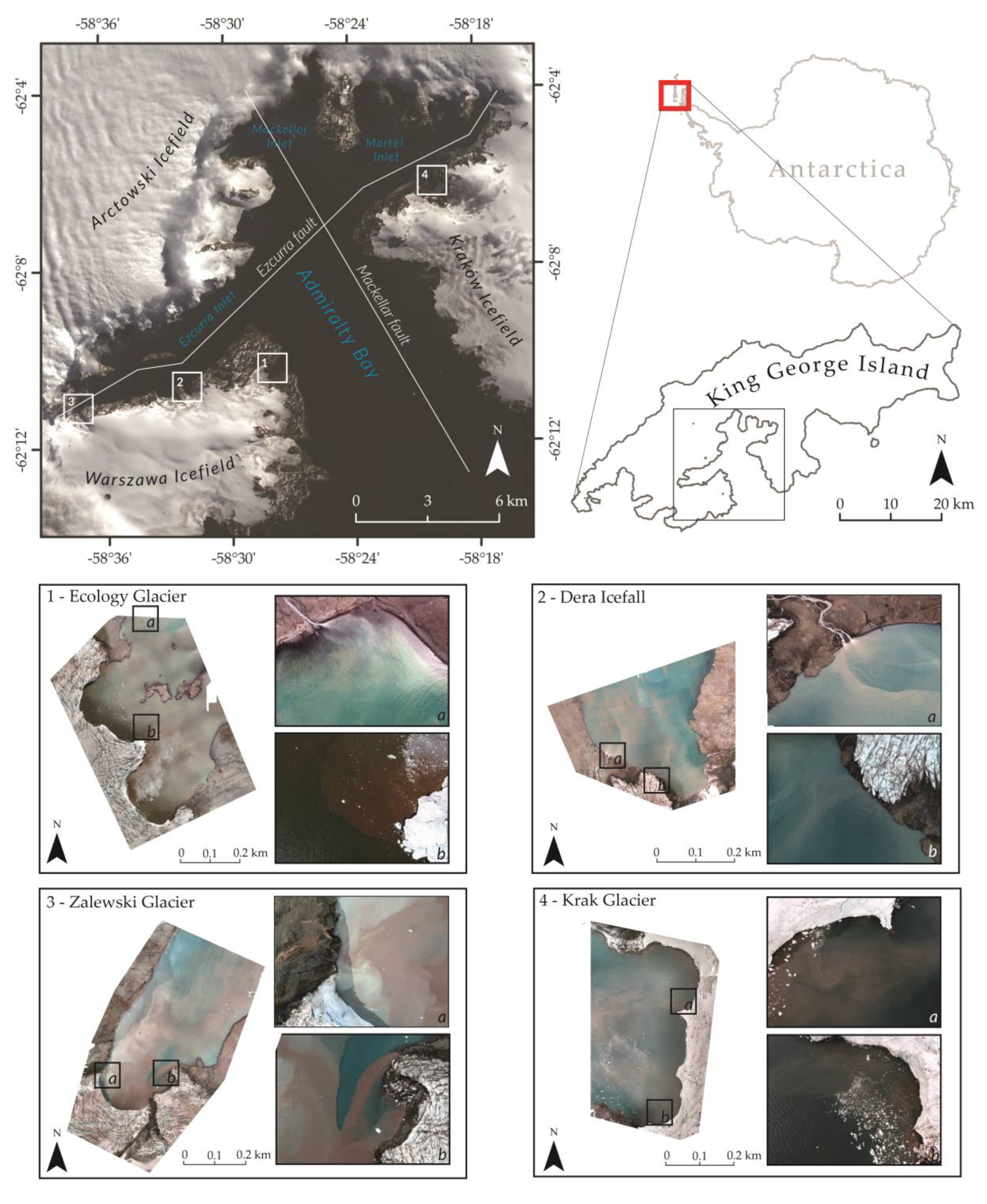
2.1. Study Area
2.2. Field Measurements
2.3. UAV Data Acquisition
2.4. Image Postprocessing
2.5. Data Analysis
3. Results
4. Discussion
5. Conclusions
Supplementary Materials
Author Contributions
Funding
Acknowledgments
Conflicts of Interest
References
- Intergovernmental Panel on Climate Change (IPCC). The latest comprehensive assessment of the state and future of the climate system, based on observations and Earth system models. In Climate Change 2013: The Physical Science Basis. Contribution of Working GroupItothe Fifth Assessment Report of the Intergovernmental Panel on Climate Change; Stocker, T.F., Qin, D., Plattner, G.-K., Tignor, M., Allen, S.K., Boschung, J., Nauels, A., Xia, Y., Bex, V., Midgley, P.M., Eds.; Cambridge University Press: Cambridge, UK, 2013. [Google Scholar]
- Rintoul, S.R.; Chown, S.L.; DeConto, R.M.; England, M.H.; Fricker, H.A.; Masson-Delmotte, V.; Naish, T.R.; Siegert, M.J.; Xavier, J.C. Choosing the future of Antarctica. Nature 2018, 558, 233–241. [Google Scholar] [CrossRef] [PubMed]
- Turner, J.; Colwell, S.R.; Marshall, G.J.; Lachlan-Cope, T.A. Antarctic climate change during the last 50 years. Int. J. Climatol. 2005, 25, 279–294. [Google Scholar] [CrossRef]
- Rückamp, M.; Braun, M.; Suckro, S.; Blindow, N. Observed glacial changes on the King George Island ice cap, Antarctica in the last decade. Glob. Planet. Chang. 2011, 79, 99–109. [Google Scholar] [CrossRef]
- Oliva, M.; Navarro, F.; Hrbáček, F.; Hernández, A.; Nývlt, D.; Pereira, P.; Ruiz-Fernández, J.; Trigo, R. Recent regional climate cooling on the Antarctic Peninsula and associated impacts on the cryosphere. Sci. Total Environ. 2017, 580, 210–223. [Google Scholar] [CrossRef] [PubMed]
- Plenzler, J.; Budzik, T.; Puczko, D.; Bialik, R.J. Climatic conditions at Arctowski Station (King George Island, West Antarctica) in 2013–2017 against the background of regional changes. Pol. Polar Res. 2019, 40, 1–27. [Google Scholar]
- Pritchard, H.D.; Vaughan, D.G. Widespread acceleration of tidewater glaciers on the Antarctic Peninsula. J. Geophys. Res. 2007, 112, 1–10. [Google Scholar] [CrossRef]
- Vaughan, D. Recent trends in melting conditions on the Antarctic Peninsula and their implications for ice-sheet mass balance and sea level. Arct. Antarct. Alp. Res. 2006, 38, 147–152. [Google Scholar] [CrossRef]
- Anderson, R.S.; Anderson, S.P. Geomorphology: The Mechanics and Chemistry of Landscapes; Cambridge University Press: Cambridge, UK, 2010. [Google Scholar]
- Hudson, B.; Overeem, I.; McGrath, D.; Syvitski, J.P.M.; Mikkelsen, A.; Hasholt, B. MODIS observed increase in duration and spatial extent of sediment plumes in Greenland fjords. Cryosphere 2014, 8, 1161–1176. [Google Scholar] [CrossRef]
- Zajączkowski, M. Sediment supply and fluxes in glacial and outwash fjords, Kongsfjorden and Adventfjorden, Svalbard. Pol. Polar Res. 2008, 29, 59–72. [Google Scholar]
- Sziło, J.; Bialik, R.J. Bedload transport in two creeks at the ice-free area of the Baranowski Glacier, King George Island, West Antarctica. Pol. Polar Res. 2017, 38, 21–39. [Google Scholar]
- Chu, V.W.; Smith, L.C.; Rennermalm, A.K.; Forster, R.R.; Box, J.E. Hydrologic controls on coastal suspended sediment plumes around the Greenland Ice Sheet. Cryosphere 2012, 6, 1–9. [Google Scholar] [CrossRef]
- Motyka, R.J.; Hunter, L.; Echelmeyer, K.A.; Connor, C. Submarine melting at the terminus of a temperate tidewater glacier, LeConte Glacier, Alaska, USA. Ann. Glac. 2003, 36, 57–65. [Google Scholar] [CrossRef]
- Pętlicki, M.; Sziło, J.; MacDonell, S.; Vivero, S.; Bialik, R.J. Recent Deceleration of the Ice Elevation Change of Ecology Glacier (King George Island, Antarctica). Remote Sens. 2017, 9, 520. [Google Scholar] [CrossRef]
- Mugford, R.I.; Dowdeswell, J.A. Modeling glacial meltwater plume dynamics and sedimentation in high-latitude fjords. J. Geophys. Res. 2011, 116. [Google Scholar] [CrossRef]
- Sziło, A.; Bialik, R.J. Grain size distribution of bedload transport in a glaciated catchment (Branowski Glacier, King George Island, Western Antarctica). Water 2018, 10, 360. [Google Scholar] [CrossRef]
- Dowdeswell, J.A.; Hogan, K.A.; Arnold, N.S.; Mugford, R.I.; Wells, M.; Hirst, J.P.P.; Decalf, C. Sediment-rich meltwater plumes and ice-proximal fans at the margins of modern and ancient tidewater glaciers: Observations and modelling. Sedimentology 2015, 62, 1665–1692. [Google Scholar] [CrossRef]
- Meredith, M.P.; Falk, U.; Bers, A.V.; Mackensen, A.; Schloss, I.R.; Ruiz Barlett, E.; Abele, D. Anatomy of a glacial meltwater discharge event in an Antarctic cove. Philos. Trans. R. Soc. A Math. Phys. Eng. Sci. 2018, 376, 20170163. [Google Scholar] [CrossRef]
- Arendt, K.E.; Dutz, J.; Jónasdóttir, S.H.; Jung-Madsen, S.; Mortensen, J.; Møller, E.F.; Nielsen, T.G. Effects of suspended sediments on copepods feeding in a glacial influenced sub-Arctic fjord. J. Plankton Res. 2011, 33, 1526–1537. [Google Scholar] [CrossRef]
- Weslawski, J.M.; Legezynska, J. Glaciers caused zooplankton mortality? J. Plankton Res. 1998, 20, 1233–1240. [Google Scholar]
- Kjelland, M.E.; Woodley, C.M.; Swannack, T.M.; Smith, D.L. A review of the potential effects of suspended sediment on fishes: Potential dredging-related physiological, behavioral, and transgenerational implications. Environ. Syst. Decis. 2015, 35, 334–350. [Google Scholar] [CrossRef]
- Fuentes, V.; Alurralde, G.; Meyer, B.; Aguirre, G.E.; Canepa, A.; Wölfl, A.C.; Schloss, I.R. Glacial melting: An overlooked threat to Antarctic krill. Sci. Rep. 2016, 6, 27234. [Google Scholar] [CrossRef] [PubMed]
- Urbanski, J.A.; Stempniewicz, L.; Węsławski, J.M.; Dragańska-Deja, K.; Wochna, A.; Goc, M.; Iliszko, L. Subglacial discharges create fluctuating foraging hotspots for sea birds in tidewater glacier bays. Sci. Rep. 2017, 7, 43999. [Google Scholar] [CrossRef] [PubMed]
- Maat, D.S.; Prins, M.A.; Brussaard, C.P. Sediments from Arctic Tide-Water Glaciers Remove Coastal Marine Viruses and Delay Host Infection. Viruses 2019, 11, 123. [Google Scholar] [CrossRef] [PubMed]
- Schild, K.M.; Hawley, R.L.; Morriss, B.F. Subglacial hydrology at Rink Isbræ, West Greenland inferred from sediment plume appearance. Ann. Glaciol. 2016, 57, 118–127. [Google Scholar] [CrossRef]
- Bhardway, A.; Joshi, P.K.; Sam, L.; Snehmani. Remote sensing of alpine glaciers in visible and infrared wavelengths: A survey of advances and prospects. Geocarto Int. 2015, 31, 557–574. [Google Scholar] [CrossRef]
- Bhardway, A.; Sam., L.; Martin-Torres, F.J.; Kumar, R. UAVs as remote sensing platform in glaciology: Present applications and future prospects. Remote Sens. Environ. 2016, 175, 196–204. [Google Scholar] [CrossRef]
- Hodgkins, R.; Bryant, R.; Darlington, E.; Brandon, M. Pre-melt-season sediment plume variability at Jökulsárlón, Iceland, a preliminary evaluation using in-situ spectroradiometry and satellite imagery. Ann. Glaciol. 2016, 57, 39–46. [Google Scholar] [CrossRef]
- Dowdeswell, J.A.; Hamilton, G.S.; Hagen, J.O. The duration of the active phase on surge-type glaciers: Contrasts between Svalbard and other regions. J. Glaciol. 1991, 37, 388–400. [Google Scholar] [CrossRef]
- Elverhøi, A.; Lønne, Ø.; Seland, R. Glaciomarine sedimentation in a modern fjord environment, Spitsbergen. Polar Res. 1983, 1, 127–150. [Google Scholar] [CrossRef]
- Dogliotti, A.I.; Ruddick, K.G.; Nechad, B.; Doxaran, D.; Knaeps, E. A single algorithm to retrieve turbidity from remotely-sensed data in all coastal and estuarine waters. Remote Sens. Environ. 2015, 156, 157–168. [Google Scholar] [CrossRef]
- Moore, G.K. Satellite remote sensing of water turbidity. Hydrol. Sci. Bull. 1980, 25, 407–421. [Google Scholar] [CrossRef]
- Garaba, S.P.; Badewien, T.H.; Braun, A.; Schuz, A.C.; Zielinski, O. Using ocean colour remote sensing products to estimate turbidity at the Wadden Sea time series station Spiekeroog. J. Eur. Opt. Soc. Rapid Publ. 2014, 9. [Google Scholar] [CrossRef]
- Odermatt, D.; Gitelson, A.; Brando, V.E.; Schaepman, M. Review of constituent retrieval in optically deep and complex from satellite imagery. Remote Sens. Environ. 2012, 118, 116–126. [Google Scholar] [CrossRef]
- Mouw, C.B.; Greb, S.; Aurin, D.; DiGiacomo, P.M.; Lee, Z.; Twardowski, M.; Binding, C.; Hu, C.; Ma, R.; Moore, T.; et al. Aquatic color radiometry remote sensing of coastal and inland waters: Challenges and recommendations for future satellite missions. Remote Sens. Environ. 2015, 160, 15–30. [Google Scholar] [CrossRef]
- Whitehead, K.; Hugenholtz, C.H. Remote sensing of the environment with small unmanned aircraft systems (UASs), part 1: A review of progress and challenges. J. Unmanned Veh. 2014, 2, 69–85. [Google Scholar] [CrossRef]
- Rymszewicz, A.; O’Sullivan, J.J.; Bruen, M.; Turner, J.N.; Lawler, D.M.; Conroy, E.; Kelly-Quinn, M. Measurement differences between turbidity instruments, and their implications for suspended sediment concentration and load calculations: A sensor inter-comparison study. J. Environ. Manag. 2017, 199, 90–108. [Google Scholar] [CrossRef]
- Pfannkuche, J.; Schmidt, A. Determination of suspended particulate matter concentration from turbidity measurements: Particle size effects and calibration procedures. Hydrol. Process. 2003, 17, 1951–1963. [Google Scholar] [CrossRef]
- Davies-Colley, R.J.; Smith, D.G. Turbidity, suspended sediment and water clarity: A review. J. Am. Water Res. Assoc. 2001, 37, 1085–1101. [Google Scholar] [CrossRef]
- Birkenmajer, K. Admiralty Bay, King George Island (South Shetland Islands, West Antarctica): A geological monograph: In Geological results of the Polish Antarctic expeditions. Studia Geol. Pol. 2003, 120, 5–73. [Google Scholar]
- Majdański, M.; Środa, P.; Malinowski, M.; Czuba, W.; Grad, M.; Guterch, A.; Hegedűs, E. 3D seismic model of the uppermost crust of the Admiralty Bay area, King George Island, West Antarctia. Pol. Polar Res. 2008, 29, 303–318. [Google Scholar]
- Commission on Standardization of Geographical Names outside the Republic of Poland (KSNG). Available online: http://ksng.gugik.gov.pl/english/index.php (accessed on 2 August 2019).
- Dera, J. Oceanographic investigation on the Ezcurra Inlet during the 2nd Antarctic Expedition of the Polish Academy of Sciences. Oceanologia 1980, 12, 5–26. [Google Scholar]
- Pruszak, Z. Currents circulation in the waters of Admiralty Bay (region of Arctowski Station on King George Island). Pol. Polar Res. 1980, 1, 55–74. [Google Scholar]
- Robakiewicz, M.; Rakusa-Suszczewski, S. Application of 3D circulation model to Admiralty Bay, King George Island, Antarctica. Pol. Polar Res. 1999, 20, 43–58. [Google Scholar]
- Braun, M.H.; Gossman, H. Glacial Changes in the Areas of Admiralty Bay and King George Island, maritime Antarctica. In Geoecology and Antarctic Ice-Free Coastal Landscapes; Beyer, L., Bülter, M., Eds.; Springer: Berlin, Germany, 2002; pp. 75–89. [Google Scholar]
- EXO User Manual. Available online: https://www.ysi.com/File%20Library/Documents/Manuals/EXO-User-Manual-Web.pdf (accessed on 8 May 2019).
- Al-amri, S.S.; Kalyankar, N.V.; Khamitkar, S.D. Linear and non-linear contrast enhancement image. Int. J. Comput. Sci. Netw. Secur. 2010, 10, 139–143. [Google Scholar]
- Hussain, M.A.; Akbari, A.S. Max-RGB based colour constancy using the sub-blocks of the image. In Proceedings of the 9th International Conference on Developments in eSystems Engineering (DeSE 2016), 31 August–2 September 2016; pp. 289–294. [Google Scholar]
- Van Groenigen, J.W.; Stein, A. Constrained Optimization of Spatial Sampling using Continuous Simulated Annealing. J. Environ. Qual. 1998, 27, 1078–1086. [Google Scholar] [CrossRef]
- Ohashi, Y.; Iida, T.; Sugiyama, S.; Aoki, S. Spatial and temporal variations in high turbidity surface water off the Thule region, northwestern Greenland. Polar Sci. 2016, 10, 270–277. [Google Scholar] [CrossRef]
- Rodrigo, C.; Giglio, S.; Varas, A. Glacier sediment plumes in small bays on the Danco Coast, Antarctic Peninsula. Antarct. Sci. 2016, 28, 395–404. [Google Scholar] [CrossRef]
- Zheng, G.; DiGiacomo, P.M. Uncertainties and applications of satellite-derived coastal water quality products. Prog. Oceanogr. 2017, 159, 45–72. [Google Scholar] [CrossRef]
- Brando, V.E.; Braga, F.; Zaggia, L.; Giardino, C.; Bresciani, M.; Matta, E.; Bellafiore, D.; Ferrarin, C.; Maicu, F.; Benetazzo, A.; et al. High-resolution satellite turbidity and sea surface temperature observations of river plume interactions during a significant flood event. Ocean Sci. 2015, 11, 909–920. [Google Scholar] [CrossRef] [Green Version]
- Quang, N.; Sasaki, J.; Higa, H.; Huan, N.H. Spatiotemporal variation of turbidity based on landsat 8 OLI in CAM Ranh Bay and Thuy Trieu Lagoon, Vietnam. Water 2017, 9, 570. [Google Scholar] [CrossRef] [Green Version]
- Yafei, L.; Doxoran, D.; Ruddick, K.; Shen, F.; Gentili, B.; Yan, L.; Huang, H. Saturation of water reflectance in extremely turbid media based on field measurments, satellite data and bio-optical modelling. Opt. Express 2018, 26, 10435–10451. [Google Scholar]
- Larson, M.D.; SimicMilas, A.; Vincent, R.K.; Evans, J.E. Multi-depth suspended sediment estimation using high-resolution remote-sensing UAV in Maumee River, Ohio. Int. J. Remote Sens. 2018, 39, 5472–5489. [Google Scholar] [CrossRef]
- Doxaran, D.; Froidefond, J.M.; Castaing, P. Remote-sensing reflectance of turbid sediment-dominated waters. Reduction of sediment type variations and changing illumination conditions effects by use of reflectance ratios. Appl. Opt. 2003, 42, 2623–2634. [Google Scholar] [CrossRef] [PubMed]
- Sokoletsky, L.; Fang, S.; Yang, X.; Wei, X. Evaluation of empirical and semianalytical spectral reflectance models for surface suspended sediment concentration in the highly variable estuarine and coastal waters of East China. IEEE J. Sel. Top. Appl. Earth Obs. Remote Sens. 2016, 9, 5182–5192. [Google Scholar] [CrossRef]
- Schild, K.M.; Hawley, R.L.; Chipman, J.W.; Benn, D.I. Quantifying suspended sediment concentration in subglacial sediment plumes discharging from two Svalbard tidewater glaciers using Landsat-8 and in situ measurements. Int. J. Remote Sens. 2017, 38, 6865–6881. [Google Scholar] [CrossRef]
- Chu, V.W.; Smith, L.C.; Rennermalm, A.K.; Forster, R.R.; Box, J.E.; Reeh, N. Sediment plume response to surface melting and supraglacial lake drainages on the Greenland ice sheet. J. Glaciol. 2009, 55, 1072–1082. [Google Scholar] [CrossRef] [Green Version]
- Ashley, G.M.; Smith, N.D. Marine sedimentation at a calving glacier margin. Geo. Soc. Am. Bull. 2000, 112, 657–668. [Google Scholar] [CrossRef]
- Hodgkins, R. Glacier hydrology in Svalbard, Norwegian high arctic. Quat. Sci. Rev. 1997, 16, 957–973. [Google Scholar] [CrossRef]
- Pan, B.J.; Vernet, M.; Reynolds, R.A.; Mitchell, B.G. The optical and biological properties of glacial meltwater in an Antarctic fjord. PLoS ONE 2019, 14, e0211107. [Google Scholar] [CrossRef] [Green Version]
- Sartori, R.Z.; Mendes, J.R.C.W.; Simões, J.C. Análise das mudançasambientais da GeleiraViéville, Baía do Almirantado, IlhaRei George, Antártica. Pesquisas em Geociências 2015, 42, 61. [Google Scholar]
- Vitti, D.M.; Marques Junior, A.; Guimaraes, T.T.; Koste, E.C.; Inocencio, L.C.; Veronez, M.R.; Mauad, F.F. Geometry accuracy of DSM in water body margin obtained from an RGB camera with NIR band and a multispectral sensor embedded in UAV. Eur. J. Remote Sens. 2018, 52, 160–173. [Google Scholar] [CrossRef] [Green Version]
- Diaz-Delgado, R.; Cazacu, C.; Adamescu, M. Rapid Assesment of Ecological Integrity for LTER Wetland Sites by Using UAV Multispectral Mapping. Drones 2019, 3, 3. [Google Scholar] [CrossRef] [Green Version]
- Kejna, M. Topoclimatic conditions in the vicinity of the Arctowski Station (King George Island, Antarctica) during the summer season of 2006/2007. Pol. Polar Res. 2008, 29, 95–116. [Google Scholar]
- Kejna, M.; Laska, K. Weather conditions at Arctowski Station, King George Island, South Shetland Islands, Antarctica in 1996. Pol. Polar Res. 1999, 20, 203–220. [Google Scholar]
- Harley, C.D.; Randall Hughes, A.; Hultgren, K.M.; Miner, B.G.; Sorte, C.J.; Thornber, C.S.; Williams, S.L. The impacts of climate change in coastal marine systems. Ecol. Lett. 2006, 9, 228–241. [Google Scholar] [CrossRef] [Green Version]


| Selected Glacier | Tectonic Formations (Birkenmajer [41]) | Geological Bedrock (Birkenmajer [41]) | Active Front Altitude (m) | Active Front Width (m)/Length of Front Adjoining Cove Waters (m) | Cove Name, Area (km2) | Sun Exposure | Glacial Retreat Ratio 1956–1995 (Braun and Gossman [47]) (%) |
|---|---|---|---|---|---|---|---|
| Ecology Glacier | Llano Point Formation (Warszawa Block) | Basalts and andesites alternating with agglomerates and tuffs | ~40 | 1185/880 | Suszczewski Cove/0.359 | NE | 5.9 |
| Dera Icefall | Point Thomas Formation (Warszawa Block) | High-aluminium basalts, breccias | - | Retreated from the waterfront | Hervé Cove/0.182 | N | 3 |
| Zalewski Glacier | Two formations divided by the Ezcurra Fault: Znosko Glacier Formation (Barton Horst)/Point Thomas Formation (Warszawa Block) | Andesites, tuffs, and agglomerates/high-aluminium basalts, breccias | ~33 | 445/255 | Unnamed Cove/0.180 | NE | 0.9, but since 1995, it has rapidly retreated further |
| Krak Glacier | Mount Wawel Formation (Warszawa Block) | Terrestrial volcanics with plant-bearing strata | max 46 | 785/785 | Lussich Cove/0.181 | NW/W | 20.9 |
| Glacier | Area Covered by the UAV Mission | Number of Photographs Taken during the Mission | Flight Altitude | Ground Sampling Distance (GSD)—Pixel Resolution | Mission Date | Tide Height during Measurements |
|---|---|---|---|---|---|---|
| Ecology | 0.23 km2 | 980 | 110 m | 11.7 cm | 26 January 2019 | 1.41 m to 1.19 m |
| Krak | 0.32 km2 | 1440 | 145 m | 15.2 cm | 31January 2019 | 0.49 m to 0.58 m |
| Zalewski | 0.33 km2 | 740 | 150 m | 15.4 cm | 28 January 2019 | 1.09 m to 0.99 m |
| 0.32 km2 | 616 | 150 m | 15.2 cm | 10 February 2019 | 1.15 m to 1.08 m | |
| Dera | 0.22 km2 | 448 | 155 m | 14.02 cm | 9 February 2019 | 0.60 m to 0.67 m |
| Glacier | Root Mean Square Error (m) | Mean Re-Projection Error (pixels) | Key Points Image Scale | |
|---|---|---|---|---|
| X | Y | |||
| Ecology | 2.15 | 2.20 | 0.525 | 9797 |
| Krak | 3.21 | 3.71 | 0.436 | 8979 |
| Zalewski 1 | 3.09 | 2.92 | 0.325 | 9067 |
| Zalewski 2 | 2.42 | 2.14 | 0.386 | 8990 |
| Dera | 2.85 | 1.90 | 0.326 | 9250 |
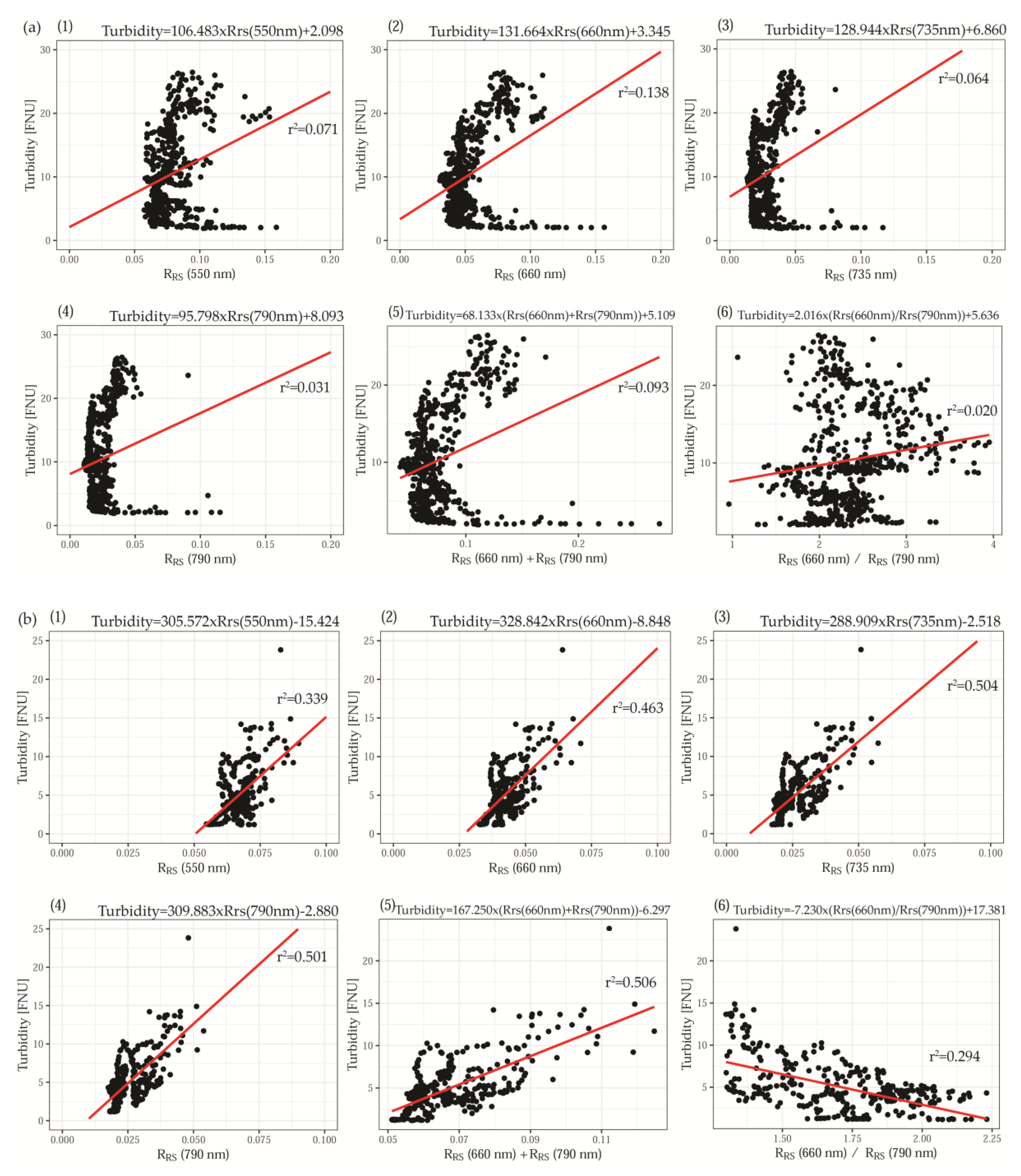
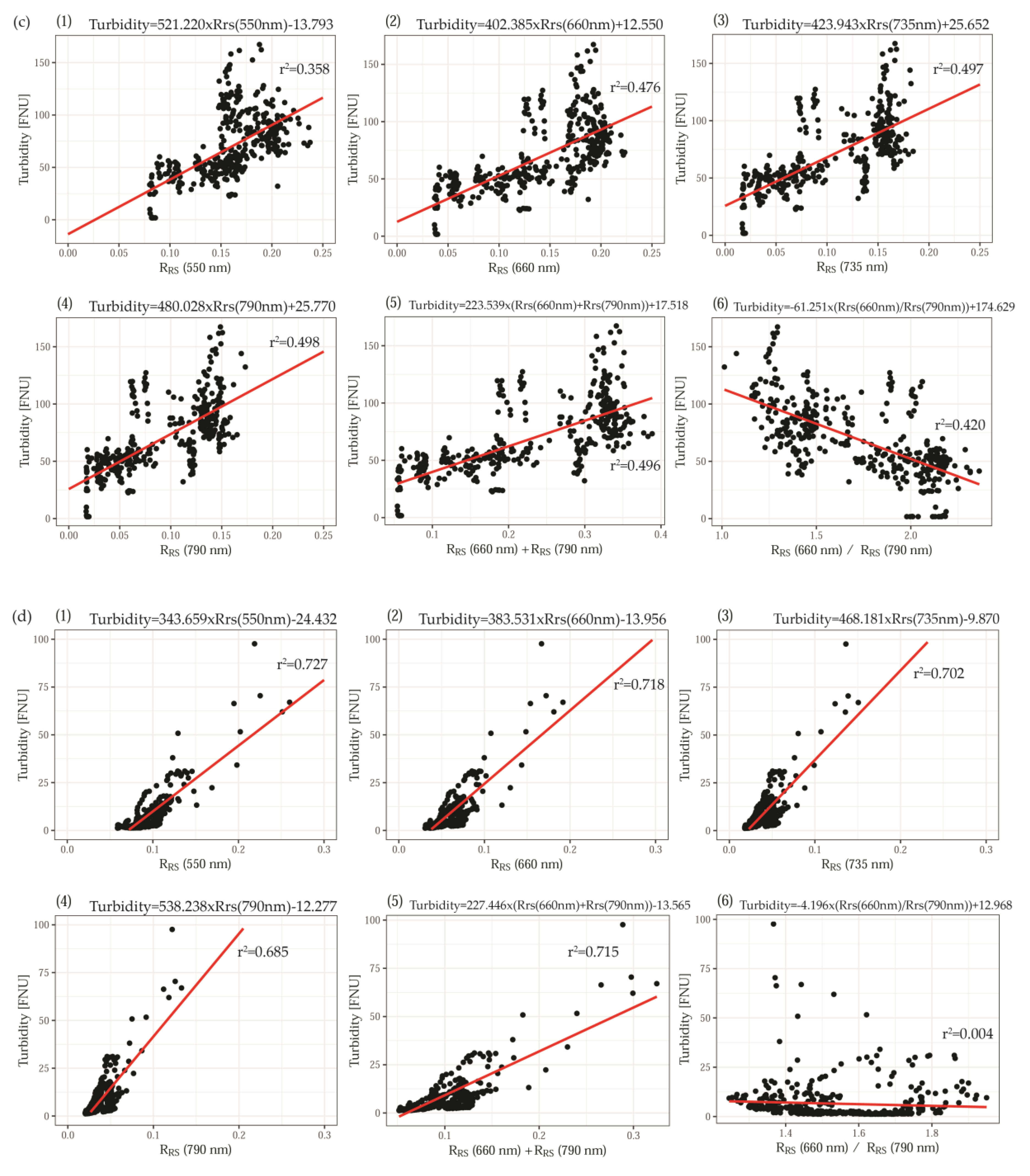
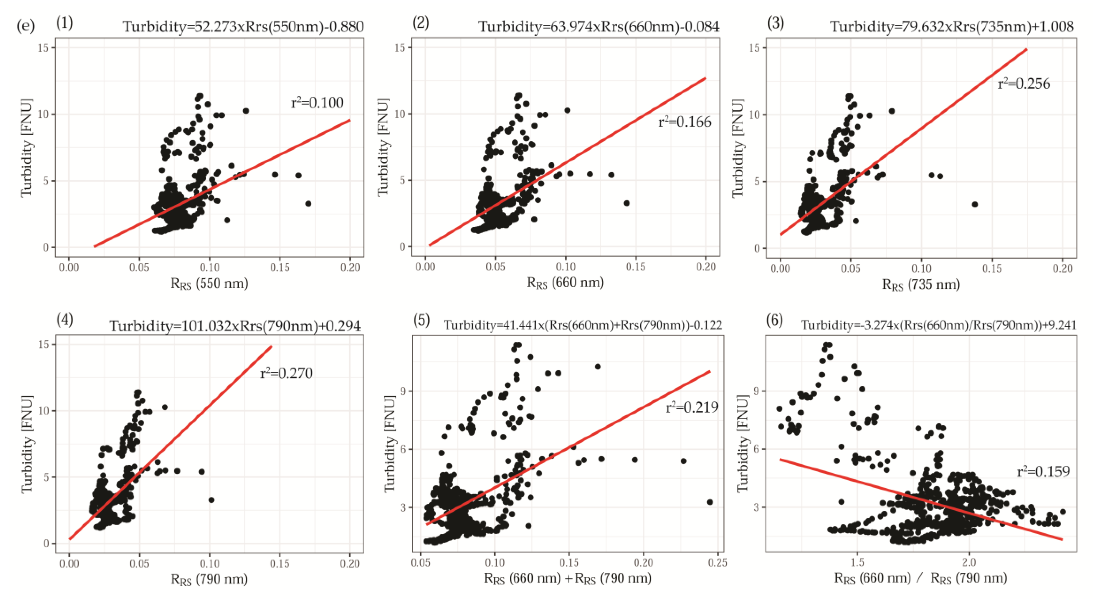
| Glacier | Number of Samples | Turbidity Range (FNU) | Spectral Region | Reflectance Range (Rrs) | r2 | P-Value | Correlation |
|---|---|---|---|---|---|---|---|
| Ecology | 638 | 1.91–26.47 | 530–570 nm | 0.02–0.32 | 0.071 | 8.85 × 10⁻¹² | 0.266 |
| 640–680 nm | 0.02–0.38 | 0.138 | 2.71 × 10⁻²² | 0.371 | |||
| 730–740 nm | 0.01–0.58 | 0.064 | 1.00 × 10⁻¹⁰ | 0.252 | |||
| 770–810 nm | 0.01–0.56 | 0.031 | 8.05 × 10⁻⁶ | 0.176 | |||
| Red + NIR | 0.02–0.80 | 0.093 | 3.02 × 10⁻¹⁵ | 0.305 | |||
| Red/NIR | 0.12–20.34 | 0.020 | 2.94 × 10⁻⁴ | 0.143 | |||
| Dera | 353 | 1.18–23.82 | 530–570 nm | 0.03–0.37 | 0.339 | 2.39 × 10⁻³² | 0.582 |
| 640–680 nm | 0.02–0.34 | 0.463 | 1.13 × 10−47 | 0.680 | |||
| 730–740 nm | 0.01–0.40 | 0.504 | 1.53 × 10−53 | 0.710 | |||
| 770–810 nm | 0.01–0.34 | 0.501 | 4.27 × 10−53 | 0.708 | |||
| Red + NIR | 0.04–0.67 | 0.506 | 8.10 × 10−54 | 0.711 | |||
| Red/NIR | 0.11–3.33 | 0.294 | 1.90 × 10⁻²⁷ | −0.542 | |||
| Zalewski 1 | 445 | 1.74–167.35 | 530–570 nm | 0.05–0.86 | 0.358 | 2.19 × 10−38 | 0.598 |
| 640–680 nm | 0.03–0.75 | 0.476 | 4.10 × 10−55 | 0.690 | |||
| 730–740 nm | 0.01–0.83 | 0.497 | 1.77 × 10−58 | 0.705 | |||
| 770–810 nm | 0.01–0.68 | 0.498 | 1.01 × 10−58 | 0.706 | |||
| Red + NIR | 0.05–1.41 | 0.496 | 2.07 × 10−58 | 0.705 | |||
| Red/NIR | 0.29–3.44 | 0.420 | 9.26 × 10−47 | −0.648 | |||
| Zalewski 2 | 451 | 1.18–97.65 | 530–570 nm | 0.03–0.62 | 0.727 | 6.39 × 10−129 | 0.853 |
| 640–680 nm | 0.03–0.57 | 0.718 | 6.82 × 10−126 | 0.848 | |||
| 730–740 nm | 0.01–0.63 | 0.702 | 2.59 × 10−120 | 0.838 | |||
| 770–810 nm | 0.02–0.55 | 0.685 | 7.44 × 10−115 | 0.827 | |||
| Red + NIR | 0.04–1.06 | 0.715 | 7.46 × 10−125 | 0.846 | |||
| Red/NIR | 0.27–6.53 | 0.004 | 1.81 × 10⁻¹ | −0.063 | |||
| Krak | 626 | 1.19–11.39 | 530–570 nm | 0.03–0.70 | 0.100 | 5.66 × 10⁻¹⁶ | 0.316 |
| 640–680 nm | 0.02–0.92 | 0.166 | 1.67 × 10⁻²⁶ | 0.408 | |||
| 730–740 nm | 0.01–1.09 | 0.256 | 5.90 × 10−42 | 0.506 | |||
| 770–810 nm | 0.01–1.10 | 0.270 | 1.47 × 10−44 | 0.519 | |||
| Red + NIR | 0.05–2.02 | 0.219 | 2.66 × 10⁻³⁵ | 0.467 | |||
| Red/NIR | 0.13–12.53 | 0.159 | 2.61 × 10⁻²⁵ | −0.399 |
© 2019 by the authors. Licensee MDPI, Basel, Switzerland. This article is an open access article distributed under the terms and conditions of the Creative Commons Attribution (CC BY) license (http://creativecommons.org/licenses/by/4.0/).
Share and Cite
Wójcik, K.A.; Bialik, R.J.; Osińska, M.; Figielski, M. Investigation of Sediment-Rich Glacial Meltwater Plumes Using a High-Resolution Multispectral Sensor Mounted on an Unmanned Aerial Vehicle. Water 2019, 11, 2405. https://0-doi-org.brum.beds.ac.uk/10.3390/w11112405
Wójcik KA, Bialik RJ, Osińska M, Figielski M. Investigation of Sediment-Rich Glacial Meltwater Plumes Using a High-Resolution Multispectral Sensor Mounted on an Unmanned Aerial Vehicle. Water. 2019; 11(11):2405. https://0-doi-org.brum.beds.ac.uk/10.3390/w11112405
Chicago/Turabian StyleWójcik, Kornelia Anna, Robert Józef Bialik, Maria Osińska, and Marek Figielski. 2019. "Investigation of Sediment-Rich Glacial Meltwater Plumes Using a High-Resolution Multispectral Sensor Mounted on an Unmanned Aerial Vehicle" Water 11, no. 11: 2405. https://0-doi-org.brum.beds.ac.uk/10.3390/w11112405