Impact of Climate Change on Water Resources in the Kilombero Catchment in Tanzania
by
 , , and
Kristian Näschen
1,* ,
,
Bernd Diekkrüger
1,
Constanze Leemhuis
2,
Larisa S. Seregina
3 and
Roderick van der Linden
3 1
Department of Geography, University of Bonn, Meckenheimer Allee 166, 53115 Bonn, Germany
2
Department of Environment and Sustainability, DLR Project Management Agency, Heinrich-Konen-Straße 1, 53227 Bonn, Germany
3
Institute of Meteorology and Climate Research, Karlsruhe Institute of Technology, 76128 Karlsruhe, Germany
*
Author to whom correspondence should be addressed.
Water 2019, 11(4), 859; https://0-doi-org.brum.beds.ac.uk/10.3390/w11040859
Submission received: 26 March 2019
/
Revised: 17 April 2019
/
Accepted: 18 April 2019
/
Published: 24 April 2019
(This article belongs to the Special Issue Hydrological and Hydro-Meteorological Extremes and Related Risk and Uncertainty)
Abstract
:This article illustrates the impact of potential future climate scenarios on water quantity in time and space for an East African floodplain catchment surrounded by mountainous areas. In East Africa, agricultural intensification is shifting from upland cultivation into the wetlands due to year-round water availability and fertile soils. These advantageous agricultural conditions might be hampered through climate change impacts. Additionally, water-related risks, like droughts and flooding events, are likely to increase. Hence, this study investigates future climate patterns and their impact on water resources in one production cluster in Tanzania. To account for these changes, a regional climate model ensemble of the Coordinated Regional Downscaling Experiment (CORDEX) Africa project was analyzed to investigate changes in climatic patterns until 2060, according to the RCP4.5 (representative concentration pathways) and RCP8.5 scenarios. The semi-distributed Soil and Water Assessment Tool (SWAT) was utilized to analyze the impacts on water resources according to all scenarios. Modeling results indicate increasing temperatures, especially in the hot dry season, intensifying the distinctive features of the dry and rainy season. This consequently aggravates hydrological extremes, such as more-pronounced flooding and decreasing low flows. Overall, annual averages of water yield and surface runoff increase up to 61.6% and 67.8%, respectively, within the bias-corrected scenario simulations, compared to the historical simulations. However, changes in precipitation among the analyzed scenarios vary between −8.3% and +22.5% of the annual averages. Hydrological modeling results also show heterogeneous spatial patterns inside the catchment. These spatio-temporal patterns indicate the possibility of an aggravation for severe floods in wet seasons, as well as an increasing drought risk in dry seasons across the scenario simulations. Apart from that, the discharge peak, which is crucial for the flood recession agriculture in the floodplain, is likely to shift from April to May from the 2020s onwards.
1. Introduction
Wetlands in East Africa cover an area of approximately 180,000 km2 [1,2] and a share of about 10% of the land surface in Tanzania, although numbers vary regarding this [3]. Nevertheless, the importance of wetlands in East Africa for the provision of numerous ecosystem services, ranging from the improvement of mental well-being [4] to water and climate regulation [5], is well proven. Yet, East African wetlands are endangered due to anthropogenic activities [6]. This pressure is driven by several push factors, such as population growth, degradation of upland soils, and increasing rainfall variability due to climate change. In contrast, wetlands have relatively fertile soils in combination with year-round water availability as pull factors for the conversion of wetlands into cropland [7,8,9,10,11]. This conversion in favor of food production consequently has negative trade-off effects on other ecosystem services.
Policies attempting to protect wetlands have often been weakly enforced [12]. Furthermore, the government of Tanzania introduced the “Kilimo Kwanza” (agriculture first), prioritizing agricultural development [13], especially in designated growth corridors. In Tanzania, the SAGCOT (Southern Agricultural Growth Corridor of Tanzania) growth corridor plays a key role. It is composed of several clusters, including the Kilombero cluster, which contains an endangered Ramsar site with considerable biodiversity resources under a condition of high stress [14]. The most important cash crop is, and will be, according to the plans of SAGCOT, rice [15]. Apart from potential ecological trade-offs due to large-scale rice production and outgrower schemes in the Kilombero area [14], analysis of the availability of water resources is inevitable to sustainably manage the highly water-dependent rice schemes. Although some research was done on water resources [16,17,18,19,20,21,22,23], the plans of SAGCOT outline future scenarios and demand wise planning, especially with regard to a changing and highly variable climate [24,25].
This work tries to bridge this research gap by simulating possible future climate scenarios with regard to water availability according to the current knowledge (regional) of climate change and hydrological modeling. Hydrological modeling in combination with climate change scenarios allows assessment of potential impacts of climate change on water resources to enable wise planning in agricultural development, as in the SAGCOT corridor, as well as for long term infrastructure projects, such as the planned dam at Stiegler’s Gorge [26], which relies to 62% on water from the Kilombero Catchment [14].
There are numerous studies worldwide on the effects of climate change on hydrology. For example, Schneider et al. [27] analyzed large scale impacts of climate change on flow regimes in Europe and found considerable changes in specific regions. The Mediterranean region will become drier due to less precipitation, while the boreal zone of northern Europe will become drier due to rising temperatures and reduced snowmelt. Nevertheless, flood peaks might be aggravated in some northern European regions due to seasonal precipitation and temperature changes. An aggravation of seasonality in streamflow was also observed for two (out of eleven) large river basins in Europe and Australia by Eisner et al. [28]. Changes in hydrology are also reported for the western United States due to changing precipitation patterns and anthropogenically-induced impacts, leading to water shortages and aggravated seasonality [29,30]. Yira et al. [31] showed that opposing discharge trends might result from the impact analysis from six climate models in a catchment in West Africa. The findings of these exemplary studies demonstrate the potential impact of climate change on hydrology through the alteration of streamflow amount and seasonality in a global context and emphasizes the nonlinear rainfall-runoff behavior, although the example’s concrete results are site specific [32]. Moreover, uncertainty and variability in climate projections, and therefore the impacts on hydrology, rise with the time horizon [33].
Several studies have also analyzed climate change in East Africa and specifically in Tanzania [24,34,35], but the implications for water resources due to climate change on a quantitative level are less well explored, particularly for the Kilombero Catchment and its surroundings. We hypothesize that the outcome of the study is helpful for water and agricultural management in the Kilombero Valley and the projections of the inflow to the planned Stiegler’s Gorge hydropower dam project.
The main objectives arising from this contextual background are the following:
- Assess the possible climatic future of the Kilombero Catchment with an emphasis on precipitation patterns and temperature variations;
- Estimate the impact of these climatic changes on hydrology by analyzing temporal and spatial changes in the water balance;
- Analyze the impact of climate change on hydrological risks, such as floods and droughts, through analyzing extreme flow situations.
These objectives are achieved by applying the well-proven hydrological model SWAT (Soil and Water Assessment Tool) in combination with an ensemble of six regional climate model simulations from the Coordinated Regional Downscaling Experiment (CORDEX) Africa project [36]. These model simulations, and furthermore different representative concentration pathways (RCPs), were utilized in the hydrological SWAT model to account for uncertainty with regard to future developments [37]. The six regional climate models were bias-corrected using local measurements to adequately represent the conditions within the catchment. The results from the SWAT model runs were analyzed with regard to general hydroclimatic patterns and extreme values, concerning peak discharge as well as low flows.
2. Materials and Methods
2.1. Study Site
The Kilombero Catchment is part of the Rufiji basin, which forms the largest river basin in Tanzania (Figure 1). The catchment is situated in the Morogoro region in southern Tanzania and comprises 40,240 km2 until its confluence with the Rufiji River. The Udzungwa Mountains in the north, with elevation ranging up to 2500 m, as well as the Mbarika Mountains and the Mahenge Highlands in the south, demarcate the border of the catchment. The Kilombero River itself receives perennial inflow mainly from the Udzungwa Mountains forming a seasonal floodplain at around 200 m above sea level (Figure 1). The floodplain itself covers an area of 7967 km2 [12], representing the biggest freshwater wetland in East Africa below 300 m above sea level [12], and is listed as an endangered Ramsar site [14]. Intensive mountainous rainfall in combination with year-round groundwater supply [23] ensure a contribution of 62% of the annual runoff volume of the Rufiji River, although the Kilombero Catchment covers only 23% of the drainage area [14].
The climate is sub-humid tropical [14] with annual mean temperatures between 24 °C in the valley and about 17 °C in the higher altitudes [14]. The areal annual precipitation amounts are between 1200 and 1400 mm [17], with a high spatio-temporal variability. The mountainous area receives up to 2100 mm precipitation, and therefore up to 1000 mm more precipitation compared to the valley [14,23]. The temporal distribution of the annual precipitation is divided into a dry season from June to November and a rainy season from November to May. Additionally, the rainy season can be split into Short Rains from November to January and Long Rains from March to May [14]. However, the interannual variability is high [38] and the reliability of the Short Rains is not as pronounced as for the Long Rains [23]. Given that some parts of the catchment lack the Short Rains, the whole catchment can be characterized by a unimodal to bimodal rainfall distribution, depending on the year and the specific area [17,39]. The main drivers of these rainfall patterns are the Intertropical Convergence Zone (ITCZ) [40] and remote forcings, such as the Walker circulation and the Indian Ocean zonal mode [41]. However, local and regional factors, such as topography and lakes, additionally influence the seasonal rainfall cycle [24]. When assessing the possible climatic future of the Kilombero Catchment, it should be noted that rainfall patterns all over East Africa are already changing at present. The long rains, which are influenced by multiple factors, such as local geographic factors, remote forcings, and regional circulations, have been declining in recent decades in eastern Africa, whereas droughts are becoming longer and increasingly stretch into the rainy seasons. Nevertheless, interannual climate variability overall for East Africa has increased in the last decades, resulting in drought periods but also unusual heavy flood events [41].
The Harmonized World Soil Database (HWSD) [42] describes the dominating soils in the valley as Fluvisols and the uplands are predominantly covered by Acrisols and Nitisols (Figure 2). In the high altitudes of the western parts of the catchment Lixisols dominate, whereas in the lower altitudes of the eastern catchment mainly Cambisols are found, according to the HWSD.
The upper catchment is dominated mainly by natural vegetation, such as tropical rainforests, bushlands, and wooded grasslands, with some patches of agricultural fields [43]. The valley contains the seasonal floodplain (Figure 1), which is characterized by rainfed lowland rice cultivation during the rainy season, whereas agriculturally undisturbed areas are dominated by grassland, such as Hyparrhenia spp., Panicum fluviicola Steud., and Phragmites mauritianus Kunth [8]. The fringes of the floodplain successively change from grassland to Miombo woodland towards the upper catchment.
Recent developments demonstrate a strong increase in population, and therefore agricultural land in the area, whereas grassland, savanna, and forested land use are declining, especially at the fringe of the wetland [14,22,23]. These anthropogenically triggered land use changes in combination with ongoing climate change might alter the hydrological system of the catchment and also affect downstream riparians. Accordingly, small-scale farmers’ food production envisioned in the planned large-scale and outgrower rice schemes of the SAGCOT growth corridor [15], as well as the planned dam at Stiegler’s Gorge [26], might presumably be influenced by changing water quantity and quality.
2.2. Input Data
This study is based on the study by Näschen et al. [23] and follows the same approach as Leemhuis et al. [22] to overcome data scarcity in the region through the application of freely available geo datasets in combination with data from local partners in Tanzania to run the hydrological model. The bottleneck to calibrate and validate the hydrological model is the discharge data for the Kilombero Catchment. Adequate discharge time series at the Swero station close to the main outlet of the catchment (Figure 1) are only available for the period of 1958–1970 (Table 1), due to the logistic challenges of the local authority Rufiji Basin Water Board (RBWB) to maintain the hydrometeorological monitoring network [13].
To gather a realistic representation of the LULC for this period, a mosaic of Landsat Level 1 images from the 1970s was classified with a supervised Random Forest classification [23,44]. Images from the whole decade were utilized due to a lack of suitable images within one single year.
Satellite rainfall estimates could not be applied in this study, due to the temporal mismatch of available discharge data (up to 1970) and satellite estimates. However, a combination of precipitation stations (Figure 1, Table 1) and modelled climate parameters from the CORDEX Africa project (Figure 1, Table 1) with a spatial resolution of 0.44° were utilized for calibration and validation of the model.
For the future climate scenarios, Regional Climate Models (RCMs) that were forced with different Global Climate Models (GCMs; Table 2) were additionally bias-corrected for precipitation and temperature to adequately represent potential changes in future climate patterns based on available data (further information in chapter 2.5). To complete the dataset for running the hydrological model, freely available datasets for the Digital Elevation Model (DEM) and the soil map (Table 1) were applied.
2.3. Model Description (SWAT Model)
The SWAT model [48] was selected in this study due to the fact that it is able to simulate hydrological processes continuously- and physically-based. These features are necessary to simulate impacts of climate change on water resources. Additionally, SWAT was already successfully calibrated and validated for the study area [23]. The model follows a semi-distributed approach by dividing the catchment into subcatchments (Figure 3) based on a threshold defined by the modeler. This threshold defines the minimum drainage area needed to generate a stream. In combination with the drainage patterns calculated from the DEM, the stream network is calculated and a subcatchment is assigned to each stream, or whenever two streams merge. In the next step, Hydrologic Response Units (HRU) divide the subcatchments into unique combinations of soil types, slope, and land use. Again the modeler has to set a minimum threshold on the absolute or relative area covered by the HRU to be included. In this study each soil type, slope class, or land use unit covering less than 10% of the area within the single subcatchments was neglected, while discretizing the subcatchments into HRUs. The model is divided into two parts. Firstly, a land phase considering all the processes from the arrival of a raindrop on the land surface until it enters the reach. From here the second phase starts, considering the routing and in-stream processes of water, sediments, nutrients, and organic chemicals. Hence, most of the hydrological processes in SWAT are calculated at the HRU level and the spatial locations of the HRUs within the subcatchments are not considered any more, but are calculated as a lumped sum of all single HRU calculations to efficiently account computationally the processes within a subcatchment.
In general, the SWAT model solves the water balance equation for each HRU and sums up the HRU calculations for each subcatchment, while integrating climate station data at the subcatchment level. The single subcatchments are linked through channel processes, which calculate the movement of water from the spatial units. Figure 3 illustrates the most important processes calculated by SWAT. For some processes, such as evapotranspiration or surface runoff, SWAT has several calculation options, but here only the applied methods to calculate the water balance are described. Precipitation is taken from single precipitation stations and is either intercepted by plants or hits the ground where it is divided into surface runoff or infiltration water by utilizing the SCS (Soil Conservation Service) curve number [49]. As long as water is near or on the surface it might evaporate according to the atmospheric conditions [50]. Once water enters the soil it might move vertically following a storage routing technique based on physical soil parameters, or laterally by using a kinematic storage model [51]. If water percolates, it passes by the unsaturated zone and enters an unconfined aquifer, from where it either leaves as capillary rise due to water demand of the surface plants, or it moves laterally as return flow into the reach. A third option is to percolate further into the confined aquifer from where the water is treated as a discharge contributor to other catchments. A more detailed description on the theoretical background is given by Neitsch et al. [52] and all the relevant model parameters are described in detail by Arnold et al. [53].
2.4. Model Setup and Evaluation (SWAT Model)
The model was setup with ArcSWAT 2012 (revision 664). Basically, the catchment was divided into 95 subcatchments consisting of 1086 HRUs. Five elevation bands [23,52] were integrated into the model due to the complex topography in combination with the sparse distribution of precipitation stations (Figure 1).
The model was calibrated and validated using SWAT-CUP (version 5.1.6.2) and the SUFI-2 algorithm [54]. Evaluation criteria were the coefficient of determination (R2; Equation (1)), the Nash-Sutcliffe efficiency (NSE; Equation (2)) and the Kling-Gupta efficiency (KGE; Equation (3)). R2 ranged between 0 and 1 (perfect fit) and both NSE and KGE ranged from −∞ to 1 (perfect fit). In this study we focus on these three criteria, as they are well-known and provide a good assessment of the model. A full description of the model setup and evaluation procedure is given by Näschen et al., 2018 [23].
Here n is the number of observations, and are the observed and simulated discharge values, respectively, and and are the mean of observed and simulated discharge values; r is the linear regression coefficient between observed and simulated data; α is the ratio of the standard deviation of simulated and observed data; β is the ratio of the means of simulated and observed data.
2.5. Climate Change Scenarios and Bias-Correction
The simulations from six CORDEX Africa RCMs were used to quantify the influence of future changes in the regional climate on the hydrology in the Kilombero Catchment. The RCMs were selected to represent the range of possible changes in seasonal rainfall amounts. Additionally, for all models two different scenarios of the Representative Concentration Pathways (RCPs) were considered. RCP4.5 and RCP8.5 assume a radiative forcing of 4.5 and 8.5 W m−2 at the end of the twenty-first century in comparison to the preindustrial level in the middle of the 19th century, respectively. The radiative forcings result from different assumptions of changes in greenhouse gas concentrations.
Systematic errors in RCM output require a comprehensive bias correction, which is based on an adjustment with respect to long-term observations. Constrained by the availability of adequate observation-based data, the bias correction could only be applied to minimum and maximum temperatures and rainfall. Due to different statistical properties and data availability, two different approaches were used for the bias correction of temperatures and rainfall.
- For the bias correction of minimum and maximum temperatures, the simple approach that was already used in a previous study [23] was adopted. In this approach, temperatures from the ERA-Interim reanalysis [55] were used as reference. Using the differences in the mean annual cycles, which were calculated from the 11-day running means of individual years between observations and model data in the period 1979–2005, model data was corrected towards observations. Due to the different representation of orography that results from the different horizontal resolutions of both datasets, i.e., 0.75° for ERA-Interim and 0.44° for CORDEX Africa RCMs, the correction was carried out for 700-hPa potential temperatures. After the correction, the RCM temperatures were transformed back to the initial level.
- Due to the non-linear statistical behavior of precipitation, a more comprehensive approach was needed for the bias correction of daily rainfall sums. All available data from seven stations in the Kilombero catchment (Figure 1) in the historical period 1951–2005 were used as reference for an empirical quantile mapping approach. In this approach the cumulative distribution function (CDF) based on simulated precipitation is adjusted towards the observation-based CDF [56]. The nearest CORDEX datagrid to the respective station was thereby utilized for the bias-correction. The usefulness of the distribution-independent quantile mapping method was demonstrated by various previous studies [31,57,58].
Assuming that the detected bias between the times series of models and observations stays spatio-temporally constant, the transfer functions found in a and b for the historical periods were applied to historical model data (1951–2005) and RCM projections (2006–2100).
2.6. Flood Frequency and Low Flow Analysis
A hydrological extreme value analysis was conducted for discharge simulated using bias-corrected RCM input to determine shifts in flood frequency and in low flows due to climatic changes. Therefore, the hydrological model was run with the historical bias-corrected RCM data for all six CORDEX Africa models (Table 2) from 1951 to 2005, as well as for the climatic projections based on the RCP 4.5 and RCP8.5 scenarios from 2010 to 2060.
Subsequently, after the model simulations, the annual maximum discharge values of the simulation periods for the six historical simulations and the RCP scenarios were extracted for further statistical analysis with regard to flood frequencies, using the extRemes 2.0 package [59] in the statistical software R. The generalized extreme value (GEV, Equations (4) and (5)) model covering Weibull, Fréchet, and Gumbel distributions was used in combination with the generalized maximum likelihood estimation (GMLE) method to estimate the return levels of flood events from 2-year return levels up to 100-year return levels. The return levels are utilized as a proxy for deviations in discharge due to climatic changes among the historical and the RCP scenarios later on.
where is the shape parameter, the location parameter, and the scale parameter of the probability distribution function with and (). If , the function belongs to the Gumbel family and is as follows:
For the low flow analysis, the Q90, being a widely-used index [60,61], was used to estimate changes among the six models and the different RCP scenarios. The Q90 index is defined here as a daily discharge value, which is exceeded in 90% of the daily simulations. These simulations were performed on decadal timescales to account for the inherent uncertainties of the scenario simulations and to identify possible decadal trends.
Additionally, the Q10 index was also calculated, which is defined here as a daily discharge value that is exceeded in 10% of the daily simulations to investigate the general flooding trend, additional to the annual maximum flooding approach based on the GEV model estimates described above. Q10 and Q90 were calculated using the hydrostats package in R [62]. The Q10 value was added to the flood frequency analysis because it is less sensitive to outliers, in contrast to the annual maximum value utilized in the GEV analysis [61].
3. Results
3.1. Model Performance
A detailed overview on the model performance is given by Näschen et al. (2018) [23]. Nevertheless, the hydrograph for the calibration and validation period is shown in Figure 4 as an important indicator for the model performance. Furthermore, common hydrological statistical measures, such as R2, NSE and KGE, are provided for both periods (Equations (1)–(3), Figure 4).
3.2. Bias-Correction
The bias-correction for all seven precipitation stations and the historic model runs for the six utilized regional climate models (Table 2) show very good results. Figure 5 shows the mean monthly precipitation for all stations and models within the period 1951–2005, with and without bias-correction. The deviation among non-bias-corrected data and the observed monthly precipitation is obvious, especially in the peak of the rainy season (March and April). Some stations indicate a shifting peak of the rainy season from April to March for all six RCMs (Figure 5c,d), in addition to these absolute deviations. Days with missing data were neglected in this analysis. In contrast to these strong deviations, Figure 5h–n shows virtually no deviations at all for the mean monthly precipitation after bias-correction.
Furthermore, the exceedance probabilities for all stations and models were analyzed (Figure 6), demonstrating a good performance of the bias-correction with regard to the cumulative distribution of rainfall events. The ensemble mean of the six models is also shown here with a completely different distribution of the ranked rainfall events, revealing a high amount of rainfall events below 10 mm, but much less events with 10 mm or more rainfall, compared to all the single model results. However, the temporal distribution of the daily rainfall patterns still varies among the observed precipitation and each single CORDEX model, apart from this ranked illustration.
A similar picture can be observed for the temperature before and after (Figure 7) bias-correction. The figure shows the mean monthly temperature for two of the 21 CORDEX datagrids (also see CORDEX datagrids in Figure 1 and Figure A1 and Figure A2) and each graph illustrates the minimum (Tmin) and maximum (Tmax) temperature of the six regional climate models. Discrepancies among all models and stations for Tmin and Tmax are obvious in Figure 7a,b, while Figure 7c,d clearly show the strong impact of the bias-correction on the mean monthly Tmin and Tmax. Only minor deviations occur in the months of April to June, which are negligible for the purpose of this study. The bias-corrected temperature data shows in general a drop in Tmin, starting with the Long Rains in March and April until the end of the rainy season in June and July. The average decrease during that time frame is about 5 °C (Table 3). From July onwards, Tmin constantly rises from about 14 °C up to 19 °C in November, and is stable henceforward until March and April again. In the dry season, Tmax increases by about 5 °C from July (23.8 °C) until November (29.3 °C) and the beginning of the Short Rains (Table 3). By then, Tmax drops again to about 25 °C on average until January and stays relatively constant between 24 and 25 °C until July (Table 3).
3.3. Climate Change Signal
Two of the most important and commonly utilized climate parameters with regard to hydrological modeling of climate change impacts are precipitation and temperature. Figure 8 displays the climate change signal of both parameters for all six RCMs by comparing the bias-corrected historical model runs with the bias-corrected projections based on the RCP scenarios in a monthly time resolution. The temperature signal (Figure 8a) generally shows a clear trend of rising temperatures between 0.5 and 2.5 °C, with the highest increase in August and September. Furthermore, the chart indicates a higher increase in the results based on the RCP8.5 projections, although model 1 and model 2, based on RCP4.5, simulate higher temperatures compared to several RCP8.5 based modeling results. Nevertheless, all model projections, except for model 6 in RCP8.5, show a constant increase of temperature throughout the year, whereas model 6 in RCP8.5 reveals an increase of less than 1 °C in January and the highest increase of about 2.5 °C in August and September, indicating the strong impact of the RCP scenarios on temperature in the dry season.
Precipitation (Figure 8b) is projected to increase according to the mean change of precipitation of all models in the two RCP scenarios. The intra-annual precipitation pattern is unaffected in the dry season. The highest increase occurs in February with 157 mm (model 6, RCP8.5), whereas the highest decrease is −47 mm in April (model 2, RCP8.5). Although the precipitation changes within the rainy season appear more complex compared to the temperature signal, some patterns are clearly visible. The months of February and March receive additional rainfall in virtually all simulations except for model 2 and 5 in RCP4.5, while the signal is much more diverse in January and April, where several models simulate decreasing rainfall. The months of May, November, and December can be seen as transition months with fewer changes in precipitation compared to the months of January to April.
3.4. Impacts of Climate Change on Water Resources
3.4.1. General Trend Analysis
The impact of the RCMs and the applied RCP scenarios on selected water balance components is shown in Table 4. The changes in precipitation indicate a dryer future according to models 2, 3, and 4, although there is a high variation with regard to these three RCMs and the two RCP scenarios, with deviations in precipitation from +22 to −109 mm per year. The projected wetter future is more consistent and pronounced with regard to models 1, 5, and 6, especially in the RCP8.5 scenario, with an annual average increase of up to 302 mm in model 6. Also, the ensemble mean scenario projects 68 mm (RCP4.5) or 88 mm additional rainfall in both RCP scenarios. The actual evapotranspiration ET0 and the water yield are also closely linked to the precipitation trends, including the surface runoff (Table 4). Hence, the trends are similar; nevertheless, the magnitude differs and is in generally more pronounced for changes in water yield in contrast to changes in ET0. The potential evapotranspiration ETp is increasing in all RCMs by 43 mm up to 136 mm.
A more detailed overview of discharge behavior in the single models and RCP scenarios is given in Figure 9 by displaying the average intra-annual discharge for the single decades from 2010 to 2060. A comparison of the single decades across the six models and two RCP scenarios displays various decades as either dry or wet. Hence, a clear signal for the discharge pattern over time is not obtained. Nevertheless, Figure 9 shows a shift of the discharge peak from April to May for all the models, except for model 3, with a shift of the peak to June, from 2020 onwards.
3.4.2. Flood Frequency and Low Flow Analysis
Figure 10 shows the return levels of flood events for all six models (Table 2) across all simulations (historical model run, RCP4.5, and RCP8.5), according to the bias-corrected CORDEX Africa data. The high variance across the six models is obvious, especially for the RCP8.5 scenarios, where the 100 year return level varies between 7782 m3 s−1 (model 5) and 20,707 m3 s−1 (model 1). Nevertheless, an increasing trend of return level values in the RCP8.5 scenario is apparent, particularly for the rare events (25 years up to 100 years), according to the simulation results. Model 5 is an exception for this finding, with rather constant return levels for a 100 year event among the scenarios.
The aforementioned results are supported by Figure 11, which displays the arithmetic mean of all scenarios for each model (Figure 11a) and the arithmetic mean of all models for the specific scenarios (Figure 11b). According to these results, model 4 and model 5 incorporate the highest and lowest return levels, respectively, with regard to 25-year return levels or higher. Figure 11b indicates a rising intensity of flooding events for the RCP4.5 and RCP8.5 scenarios.
Table 5 confirms the finding that the impact of RCP scenarios regarding a rise of flood magnitudes increases with increasing return periods. The relative change of all models and RCP scenario runs in comparison to their respective historical simulations is shown for the single return periods. The arithmetic mean of the percentage increase of the return levels rises constantly, while the standard deviation rises from the 5 year return level upwards, even though relative changes with increasing discharge values are considered as a baseline in these calculations.
Figure 12 shows Q10 and Q90, representing the high flow and low flow conditions for the historic model runs and the future scenarios for each model. The historic model runs are only represented by one value (dashed lines) for the entire simulation period of each model, whereas the RCP scenario simulations contribute decadal values from 2010 to 2060 for both RCP scenarios, to concentrate on future climate developments. The difference among the six models for Q10 and Q90 is obvious. Models 2 and 3 have comparably low Q10 and Q90 values, while models 1, 4, and 6 have comparably high Q10 values. Q90 values for models 1, 4, 5 and 6 are similar, and all simulated Q90 values are below the measured historical Q90. A more detailed analysis is given in Figure 13, which accounts for the decadal shifts of Q10 and Q90 in a Cartesian coordinate system. The changes in m3 s−1 for both RCP scenario simulations of the RCMs on a decadal basis are given in comparison to the historic Q10 and Q90 values of the respective model. For example, a red “2” in the bottom left quadrant refers to a RCP8.5 (red color) scenario simulation from 2020 to 2029 and represents decreasing Q90 (below zero line) and decreasing Q10 amounts (left to the zero line). A blue “5” in the top right quadrant refers to a RCP4.5 (blue color) scenario simulation from 2050 to 2059 and represents increasing Q90 (above zero line) and increasing Q10 amounts (right to the zero line).
After integrating all results a linear trend is obvious, with coinciding trends of decreasing Q10 and Q90 or increasing Q10 and Q90. Nevertheless, a few examples are located in the top left quadrant of the coordinate system, representing slightly increasing Q90, whereas Q10 is decreasing. Both RCP scenarios and simulations from the 2020s, 2030s, and 2050s show this pattern (Figure 13; blue and red “2”, “3”, and “5” in top left quadrant). The most extreme simulations with the highest changes for Q10 and for Q90 are within the RCP8.5 scenario, with one exception. In the 2050s there is a huge reduction (−706 m3 s−1) in Q10 for one of the RCP4.5 scenarios (model 3) simulated. In general, most of the scenarios show a wetter future, represented by the accumulation of changes in Q10 and Q90 in the top right quadrant (Figure 13).
This general trend towards a wetter future is also represented in the results of smaller spatial scale (Figure 14). Figure 14 displays the comparison of the wettest and driest decade with their respective historical model run (1951–2005) for the overall water yield and evapotranspiration. Model 2 under the RCP8.5 scenario for the period 2020–2029 and model 6 under the RCP8.5 scenario for the period 2040–2049 were identified as the driest and wettest decades with regard to changes in discharge. This finding is based on the general hydrograph analysis (Figure 9) and the behavior of extreme discharge represented by Q10 and Q90 (Figure 13). The very pronounced increase of the overall water yield in the “wet scenario” (Figure 14a) is obvious, whereas the decrease in the “dry scenario” (Figure 14b) is less pronounced. The difference between the wet and dry scenarios with regard to evapotranspiration (Figure 14c,d) is more balanced and has a smaller magnitude. The changes in water balance components are less distinctive in the western part of the catchment for both scenarios compared to the eastern part of the catchment.
4. Discussion
4.1. Model Performance and Bias-Correction
The performance of the model and the arising uncertainties due to the data scarcity in the region are discussed in detail by Näschen et al. [23]. Hence, only a brief discussion on model performance is given here, whereas the main interest is drawn to the bias correction of the climate data, namely precipitation and temperature data.
The discharge pattern for the calibration and validation period (Figure 4) is captured well, with a good to very good statistical performance, according to Moriasi et al. [63]. Deductions in statistical performance can be attributed to overestimations of discharge in some years (1959, 1961) and inaccuracies in simulating the discharge peaks [23]. During calibration, five out of the seven most sensitive parameters were related to groundwater [23], indicating the importance of groundwater contribution for the catchment, which was also highlighted by other researchers [21,64].
Bias-corrections with quantile mapping worked very well, as already proven by Teng et al. [65] in a comparison of several bias−correction methods. The seasonal variability for rainfall on monthly scale (Figure 5), as well as the exceedance probabilities of the bias-corrections, perform very well (Figure 6). The ensemble mean simulations of rainfall were neglected in this study due to their huge deviations compared to the single model outputs, with regard to the ranked rainfall distribution (Figure 6). Bias correction for temperature was also successful for all 21 CORDEX Africa datagrids, which is obvious by comparing Figure 7a–d, as well as Figure A1 and Figure A2. The average annual temperature cycle (Table 3) displays a typical tropical daytime climate, indicated by more pronounced daily temperature amplitudes of up to 11.7 °C in September as an average of the whole period and all stations. However, the seasonal cycle is evident with Tmax and Tmin differences of up to 5.5 °C among the lowest and highest areal mean values within the considered period. Hence, it has to be considered that the bias correction was done from the period 2006 to 2100, but the analyses were only done until 2060 to find a compromise between the statistical variability of climate change projections and planning time-frames, such as the Tanzania Vision 2025.
The behavior of the areal mean monthly temperature of the catchment (Figure 7, Table 3) fits very well to the temporal precipitation patterns and the onset and ending of dry and rainy seasons [17,23]. Minimum temperatures decrease from March until July, which can be attributed to cooling by evapotranspiration and shifts in the share of sensible and latent heat transport [66]. In July, minimum temperature starts to rise again from about 14 °C to 19 °C, while maximum temperatures simultaneously increase from July until November, which is the onset of the short rains, where again cooling is achieved via evapotranspiration as well as more pronounced cloud coverage, and therefore less solar radiation [67]. The increase of minimum and maximum temperatures starting in July also fits well with the declining impact of cooling by evapotranspiration within the catchment. It was shown [23] that actual evapotranspiration and potential evapotranspiration diverge from July onwards due to a water deficit. This is exactly the month where minimum and maximum temperatures begin to rise, due to an increasing share of sensible heat in combination with decreasing cloud coverage. The reduced cloud coverage also implies a higher radiation and a positive feedback with regard to temperature in a drying system [68]. The bias-corrected climate data, therefore, represent a sound behavior of a seasonal sub-humid tropical system. Moreover, water availability in the system is indirectly well-reflected by the shift in actual and potential evapotranspiration.
4.2. Impact of Climate Change on Water Resources
Overall, the modeled scenarios project a broad range of dry and wet conditions, whereas the distinction towards a wetter future for the catchment is more pronounced (Table 4, Figure 13). The annual average change in precipitation ranges between a reduction by 109 mm and an increase by 302 mm with respect to historical model runs, with an annual mean of 1336 mm. The rising temperature in all models, due to the adopted RCP scenarios, leads to consistently increasing potential evapotranspiration, while water availability is a temporally limiting factor due to the distinct seasonality in the catchment [17,38].
This limitation of water is visible by looking at the changes in actual and potential evapotranspiration in the RCM projections. Potential evapotranspiration is increasing in all projections (Table 4), whereas the development of the actual evapotranspiration is more variable, indicating a spatio-temporal water deficit. On the one hand, dry scenario simulations (e.g., model 3 in RCP8.5; see Table 4) show increasing actual evapotranspiration, although precipitation is decreasing. This can be attributed to both increasing potential evapotranspiration and decreasing water yields. On the other hand, the increase of actual evapotranspiration is less distinctive in the wet scenarios (models 1, 5, 6) in comparison to the increase of precipitation (e.g., models 1 and 6 in both scenarios; see Table 4). In these scenarios, surface runoff increases by up to 67.8% and the overall water yield by up to 61.6%, indicating a shift in water balance, favoring water yield instead of evapotranspiration. This shift might be attributed to the temporal distribution of the precipitation. Figure 8 shows the increase of rainfall within the rainy season, while the temperature, and therefore the potential evapotranspiration, rises, especially in the dry season. Additionally, the aforementioned models 1, 5, and 6 show comparably high values of Q10 (Figure 12a,b), implying higher discharge peaks and heavy rainfall events. Furthermore, it was already shown that the system is energy limited throughout the rainy season, with actual evapotranspiration equal to potential evapotranspiration [23]. Otherwise, there is distinct water limitation throughout the dry season, with Q90 values below the historical measured value (Figure 12c,d).
An overall aggravation of seasonality is particularly challenging in (East) African countries because of the already existing high spatial and temporal variability of available water resources [69]. Considering the climatic feedback described in chapters 3.4 and 4.1, including the rising temperatures in combination with decreasing low flow and water availability in the dry season, drought-related risks might be aggravated in the region due to climate change. However, flooding intensity is more likely to increase (Figure 11b, Figure 13). This indicates an aggravation of severe floods in the rainy season in combination with the chance of an increasing drought risk in the dry season. Additionally, the discharge peak and the following inundation, which are important factors for the recession agriculture in the valley [17,70], are likely to shift from April to May from the 2020s onwards (Figure 9). This shift might be attributed to the changing precipitation patterns (Figure 8b) in combination with the comparably slow drainage for the overall catchment [16]. Therefore, wise catchment management is needed to adequately use and retain the potentially occurring water benefit in the rainy season and make it available during the more pronounced drought periods in the dry season. In contrast, poorly adapted catchment management will increase the risk of severe floods. Additionally, a shift in inundation dynamics needs to be communicated to ensure efficient agricultural production.
Although results show no clear signal towards an extension or shortening of the dry or wet seasons across all models, precipitation amounts primarily increase within the rainy season. In contrast, the dry season from June to October is consistent with regard to very low precipitation amounts (<20 mm per month on average) and increasing potential evapotranspiration due to increasing temperatures, even though some regional climate models predict increasing rainfall in September (Figure 8). However, a general consistency within the single scenarios regarding extreme events is observed, with an antagonistic trend of either a decrease of both Q10 and Q90 or the opposite trend, with only a few less-pronounced exceptions (Figure 13).
Nevertheless, the wide distribution of the decadal simulation results and also the RCM simulation results in Figure 13 show that the occurrence of a trend towards a wetter future with regard to Q10 and Q90 is more likely. However, the spread of the different models and the decadal distribution indicate a high uncertainty and no clear temporal trend. Especially, the span for extreme events, e.g., the 100-year return level, between the six models is extremely high (Figure 10, Table 5) and results have to be considered carefully. This span can be taken as a range of uncertainty, with a set of possible futures scenarios for the Kilombero Catchment. The knowledge of the performance of these climate scenarios and models can be very useful for management purposes of the catchment, e.g., the estimation of future inundation dynamics. Therefore, a hydraulic model for the agriculturally utilized parts of the catchment needs to be established to estimate the impacts of potential scenarios. The analyses in Figure 11a and Figure 12a,b suggest utilizing either model 1, 3, 4, or 6 in hydraulic flood models to prepare for possible future flooding events under wetter conditions and changing inundation dynamics, due to the high return levels and Q10 values. In contrast to that, model 2 and model 3 are suitable to prepare for dry conditions, for example in environmental flow assessments.
A more detailed analysis has already been undertaken by investigating the impact of particular wet and dry decades and their impact on water balance components (Figure 14). There exists a distinctive increase of the overall water yield in the wet scenario, resulting in an increase of about 50% within nearly all subcatchments compared to the status quo [23]. This change will have a huge impact on the overall hydrology of the catchment and its management. On the one hand, this is only the annual average of a whole decade, and therefore conceals intra- and interannual dynamics, which are even more pronounced. On the other hand, one has to keep in mind that this is the most extreme scenario out of many possible future scenarios. Nevertheless, the comparison of these extreme scenarios provides a sense of the uncertainty that water management has to deal with. The distinct influence of both the driest and wettest simulated decades on the eastern part of the catchment (Figure 14) can be attributed to the fact that the eastern part is, in general, more important for the water yield of the catchment due to the precipitation patterns and also the direction of flow of the Kilombero River towards the east [23]. Nathkin et al. [35] give an overview of studies investigating the impact of climate on discharge regimes. They also show diverging effects of climate change on discharge regimes, but most of the studies imply a decrease of discharge in the dry season in contrast to an increasing total runoff, which is in line with the insights in this study. Reasons for changes in the discharge regimes are changes in precipitations patterns [71,72], increasing evapotranspiration due to higher temperature [72], LULC changes [71], water abstractions [72,73], and dam constructions [74].
These study results show that in addition to climate change analyses, manifold factors are influencing the hydrology within the catchment [75]. The method of land use and management, for example, exerts strong influence over soil hydraulic properties, and thus influences the amount of water retention, surface runoff, and flood generation [76,77]. Particularly, agricultural land is characterized by high degrees of soil cultivation and low soil coverage by vegetation during parts of the year, which in general leads to an increase of surface runoff generation. Thus, a growth of the share of agricultural land, which is promoted through the SAGCOT initiative [15], might lead to an aggravation of flood events, and hence intensify the negative effects climate change might exert on the regional water balance. Apart from the presumable effects on water balance, an increment in agricultural area might also lead to biodiversity losses within the Ramsar site [8,78].
Still, the extent to which increasing agricultural production influences soil hydraulic properties depends on different regionally varying factors, such as soil type, cultivation, and irrigation schemes, and location within the catchment. The aforementioned factors need to be determined within proper field studies to assist in planning for the future water resource management of the Kilombero Catchment.
In general, LULC change [79] and management change scenarios should be developed and included in future analyses to investigate their combined impact in combination with climate change on water resources. Moreover, this study concentrates only on water quantity, due to the lack of data on water quality, but it was already demonstrated that the impact of climate change could be amplified by LULC change with regard to soil erosion and the accompanied nutrient input into surface waters [80,81].
5. Conclusions
The study clearly showed the broad range of possible future climate scenarios for the Kilombero Catchment according to the bias-corrected CORDEX Africa projections. The climate impact analysis on hydrology recommends adapting to more distinct seasonality due to shifting rainfall patterns. These shifting patterns will probably result in changing inundation dynamics and more severe flooding, while the likelihood of decreasing low flows is less pronounced. The designation of suitable arable land for the recession agriculture has to be adjusted in accordance with the respective hydrological patterns. Future agricultural management strategies should also take into account a delay of approximately one month in the inundation of the floodplain within the next decades, because of the common delay signal across all simulations (Figure 9). The presented modeling results should be taken as a range of possible futures, which could be applied following the precautionary principle to assess and prepare for possible future conditions. However, it is strongly recommended to use these climate change scenarios in combination with LULC change scenarios and management scenarios to have a more realistic representation of the hydrological conditions. These hydrological model results should be implemented into a well-established hydraulic model to get a better understanding of their possible impact on inundation extent, depth, and timing. This will facilitate and enhance the management of the floodplain and might assist in the designation of suitable areas for either conservation measures or agricultural production zones, also with regard to downstream water users and water-related infrastructure, such as the planned hydropower dam at Stiegler’s Gorge.
Author Contributions
K.N., B.D. and C.L. conceived and designed the experiments. K.N. performed the experiments. K.N. and B.D. analyzed the data. R.v.d.L. and L.S.S. downloaded and bias-corrected the climate data. K.N. wrote the article. All authors made revisions and improvements to the final version.
Funding
This study was supported through funding from the German Federal Ministry of Education and Research (FKZ: 031A250A−H) and German Federal Ministry for Economic Cooperation and Development under the “GlobE: Wetlands in East Africa” project.
Acknowledgments
The authors would like to thank the Rufiji Basin Water Board for data sharing and assistance in the field and Salome Misana for her administrative guidance and logistic assistance.
Conflicts of Interest
The authors declare no conflict of interest. The funding sponsors had no role in the design of the study; in the collection, analyses, or interpretation of data; in the writing of the manuscript; or in the decision to publish the results.
Appendix A
Figure A1.
Temperature from 1979–2005 for the 21 utilized CORDEX Africa datagrids before bias-correction. Each graph shows the average monthly temperature for all six models introduced in Table 2. Tmin and Tmax represent the mean monthly minimum and maximum temperatures respectively.
Figure A1.
Temperature from 1979–2005 for the 21 utilized CORDEX Africa datagrids before bias-correction. Each graph shows the average monthly temperature for all six models introduced in Table 2. Tmin and Tmax represent the mean monthly minimum and maximum temperatures respectively.

Figure A2.
Temperature from 1979–2005 for the 21 utilized CORDEX Africa datagrids after bias-correction with Era-Interim data. Each graph shows the average monthly temperature for all six models after bias-correction in Table 2. Tmin and Tmax represent the mean monthly minimum and maximum temperatures respectively.

References
- Leemhuis, C.; Amler, E.; Diekkrüger, B.; Gabiri, G.; Näschen, K. East African wetland-catchment data base for sustainable wetland management. Proc. Int. Assoc. Hydrol. Sci. 2016, 374, 123–128. [Google Scholar] [CrossRef]
- Stevenson, N.; Frazier, S. Review of wetland inventory information in Africa. In Global Review of Wetland Resources and Priorities for Wetland Inventory; Spiers, A.G., Finlayson, C.M., Eds.; Supervising Scientist: Canberra, Australia, 1999; pp. 105–201. [Google Scholar]
- Amler, E.; Schmidt, M.; Menz, G. Definitions and Mapping of East African Wetlands: A Review. Remote Sens. 2015, 7, 5256–5282. [Google Scholar] [CrossRef] [Green Version]
- Heinkel, S.B. Therapeutic Effects of Wetlands on Mental Well-Being. The Concept of Therapeutic Landscapes Applied to an Ecosystem in Uganda. Ph.D. Thesis, University of Bonn, Bonn, Germany, 2018. [Google Scholar]
- Maltby, E.; Acreman, M. Ecosystem services of wetlands: Pathfinder for a new paradigm. Hydrol. Sci. J. 2011, 56, 1341–1359. [Google Scholar] [CrossRef]
- Gardner, R.C.; Finlayson, C.M. Global Wetland Outlook: State of the World’s Wetlands and Their Services to People; The Ramsar Convention Secretariat: Gland, Switzerland, 2018. [Google Scholar]
- Beuel, S.; Alvarez, M.; Amler, E.; Behn, K.; Kotze, D.; Kreye, C.; Leemhuis, C.; Wagner, K.; Willy, D.K.; Ziegler, S.; et al. A rapid assessment of anthropogenic disturbances in East African wetlands. Ecol. Indic. 2016, 67, 684–692. [Google Scholar] [CrossRef]
- Behn, K.; Becker, M.; Burghof, S.; Möseler, B.M.; Willy, D.K.; Alvarez, M. Using vegetation attributes to rapidly assess degradation of East African wetlands. Ecol. Indic. 2018, 89, 250–259. [Google Scholar] [CrossRef]
- Kirimi, F.; Thiong, K.; Gabiri, G.; Diekkrüger, B. Assessing seasonal land cover dynamics in the tropical Kilombero floodplain of East Africa. J. Appl. Remote Sens. 2018, 12, 026027. [Google Scholar] [CrossRef]
- Gabiri, G.; Diekkrüger, B.; Leemhuis, C.; Burghof, S.; Näschen, K.; Asiimwe, I.; Bamutaze, Y. Determining hydrological regimes in an agriculturally used tropical inland valley wetland in central Uganda using soil moisture, groundwater, and digital elevation data. Hydrol. Process. 2017, 32, 349–362. [Google Scholar] [CrossRef]
- Rebelo, L.M.; McCartney, M.P.; Finlayson, C.M. Wetlands of Sub−Saharan Africa: Distribution and contribution of agriculture to livelihoods. Wetl. Ecol. Manag. 2010, 18, 557–572. [Google Scholar] [CrossRef]
- Mombo, F.; Speelman, S.; Huylenbroeck, G.V.; Hella, J.; Moe, S. Ratification of the Ramsar convention and sustainable wetlands management: Situation analysis of the Kilombero Valley wetlands in Tanzania. J. Agric. Ext. Rural Dev. 2011, 3, 153–164. [Google Scholar]
- Munishi-Kongo, S. Ground and Satellite-Based Assessment of Hydrological Responses To Land Cover Change in the Kilombero River Basin, Tanzania. Ph.D. Thesis, University of KwaZulu-Natal, Durban, South Africa, 2013. [Google Scholar]
- Wilson, E.; McInnes, R.; Mbaga, D.P.; Ouedaogo, P. Ramsar Advisory Mission Report: United Republic of Tanzania, Kilombero Valley; The Ramsar Convention Secretariat: Gland, Switzerland, 2017. [Google Scholar]
- Government of Tanzania. Southern Agricultural Growth Corridor of Tanzania (SAGCOT): Environmental and Social Management Framework (ESMF); Government of Tanzania: Dar es Salaam, Tanzania, 2013.
- Lyon, S.W.; Koutsouris, A.; Scheibler, F.; Jarsjö, J.; Mbanguka, R.; Tumbo, M.; Robert, K.K.; Sharma, A.N.; van der Velde, Y. Interpreting characteristic drainage timescale variability across Kilombero Valley, Tanzania. Hydrol. Process. 2015, 29, 1912–1924. [Google Scholar] [CrossRef]
- Koutsouris, A.J.; Chen, D.; Lyon, S.W. Comparing global precipitation data sets in eastern Africa: A case study of Kilombero Valley, Tanzania. Int. J. Climatol. 2016, 36, 2000–2014. [Google Scholar] [CrossRef]
- Burghof, S. Hydrogeology and water quality of wetlands in East Africa. Ph.D. Thesis, University of Bonn, Bonn, Switzerland, 2017. [Google Scholar]
- Daniel, S.; Gabiri, G.; Kirimi, F.; Glasner, B.; Näschen, K.; Leemhuis, C.; Steinbach, S.; Mtei, K. Spatial Distribution of Soil Hydrological Properties in the Kilombero Floodplain, Tanzania. Hydrology 2017, 4, 57. [Google Scholar] [CrossRef]
- Yawson, D.K.; Kongo, V.M.; Kachroo, R.K. Application of linear and nonlinear techniques in river flow forecasting in the Kilombero River basin, Tanzania. Hydrol. Sci. J. 2005, 50, 37–41. [Google Scholar] [CrossRef]
- Gabiri, G.; Burghof, S.; Diekkrüger, B.; Steinbach, S.; Näschen, K. Modeling Spatial Soil Water Dynamics in a Tropical Floodplain, East Africa. Water 2018, 10, 191. [Google Scholar] [CrossRef]
- Leemhuis, C.; Thonfeld, F.; Näschen, K.; Steinbach, S.; Muro, J.; Strauch, A.; López, A.; Daconto, G.; Games, I.; Diekkrüger, B. Sustainability in the food-water-ecosystem nexus: The role of land use and land cover change for water resources and ecosystems in the Kilombero Wetland, Tanzania. Sustainability 2017, 9, 1513. [Google Scholar] [CrossRef]
- Näschen, K.; Diekkrüger, B.; Leemhuis, C.; Steinbach, S.; Seregina, L.; Thonfeld, F.; van der Linden, R. Hydrological Modeling in Data-Scarce Catchments: The Kilombero Floodplain in Tanzania. Water 2018, 10, 599. [Google Scholar] [CrossRef]
- Seregina, L.S.; Fink, A.H.; van der Linden, R.; Elagib, N.A.; Pinto, J.G. A new and flexible rainy season definition: Validation for the Greater Horn of Africa and application to rainfall trends. Int. J. Climatol. 2018, 39, 898–1012. [Google Scholar] [CrossRef]
- Koutsouris, A. Building a coherent hydro-climatic modelling framework for the data limited Kilombero Valley of Tanzania. Ph.D. Thesis, Stockholm University, Stockholm, Sweden, 2017. [Google Scholar]
- Duvail, S.; Mwakalinga, A.B.; Eijkelenburg, A.; Hamerlynck, O.; Kindinda, K.; Majule, A. Jointly thinking the post-dam future: Exchange of local and scientific knowledge on the lakes of the Lower Rufiji, Tanzania. Hydrol. Sci. J. 2014, 59, 713–730. [Google Scholar] [CrossRef]
- Schneider, C.; Laizé, C.L.R.; Acreman, M.C.; Flörke, M. How will climate change modify river flow regimes in Europe? Hydrol. Earth Syst. Sci. 2013, 17, 325–339. [Google Scholar] [CrossRef] [Green Version]
- Eisner, S.; Flörke, M.; Chamorro, A.; Daggupati, P.; Donnelly, C.; Huang, J.; Hundecha, Y.; Koch, H.; Kalugin, A.; Krylenko, I.; et al. An ensemble analysis of climate change impacts on streamflow seasonality across 11 large river basins. Clim. Chang. 2017, 141, 401–417. [Google Scholar] [CrossRef]
- Barnett, T.P.; Pierce, D.W.; Hidalgo, H.G.; Bonfils, C.; Santer, B.D.; Das, T.; Bala, G.; Wood, A.W.; Nozawa, T.; Mirin, A.A.; et al. Human-induced changes in the hydrology of the western United States. Science 2008, 319, 1080–1083. [Google Scholar] [CrossRef]
- Barnett, T.P.; Adam, J.C.; Lettenmaier, D.P. Potential impacts of a warming climate on water availability in snow-dominated regions. Nature 2005, 438, 303–309. [Google Scholar] [CrossRef]
- Yira, Y.; Diekkrüger, B.; Steup, G.; Bossa, A.Y. Impact of climate change on hydrological conditions in a tropical West African catchment using an ensemble of climate simulations. Hydrol. Earth Syst. Sci. 2017, 21, 2143–2161. [Google Scholar] [CrossRef]
- Feng, D.; Beighley, E.; Raoufi, R.; Melack, J.; Zhao, Y.; Iacobellis, S.; Cayan, D. Propagation of future climate conditions into hydrologic response from coastal southern California watersheds. Clim. Chang. 2019, 153, 199–218. [Google Scholar] [CrossRef]
- Gelfan, A.; Gustafsson, D.; Motovilov, Y.; Arheimer, B.; Kalugin, A.; Krylenko, I.; Lavrenov, A. Climate change impact on the water regime of two great Arctic rivers: Modeling and uncertainty issues. Clim. Chang. 2017, 141, 499–515. [Google Scholar] [CrossRef]
- Lalika, M.C.S.; Meire, P.; Ngaga, Y.M.; Chang’a, L. Understanding watershed dynamics and impacts of climate change and variability in the Pangani River Basin, Tanzania. Ecohydrol. Hydrobiol. 2015, 15, 26–38. [Google Scholar] [CrossRef]
- Natkhin, M.; Dietrich, O.; Schäfer, M.P.; Lischeid, G. The effects of climate and changing land use on the discharge regime of a small catchment in Tanzania. Reg. Environ. Chang. 2015, 15, 1269–1280. [Google Scholar] [CrossRef]
- Gutowski, J.W.; Giorgi, F.; Timbal, B.; Frigon, A.; Jacob, D.; Kang, H.S.; Raghavan, K.; Lee, B.; Lennard, C.; Nikulin, G.; et al. WCRP COordinated Regional Downscaling EXperiment (CORDEX): A diagnostic MIP for CMIP6. Geosci. Model Dev. 2016, 9, 4087–4095. [Google Scholar] [CrossRef]
- Moss, R.H.; Edmonds, J.A.; Hibbard, K.A.; Manning, M.R.; Rose, S.K.; van Vuuren, D.P.; Carter, T.R.; Emori, S.; Kainuma, M.; Kram, T.; et al. The next generation of scenarios for climate change research and assessment. Nature 2010, 463, 747–756. [Google Scholar] [CrossRef]
- Nicholson, S.E. The nature of rainfall variability over Africa on time scales of decades to millenia. Glob. Planet. Chang. 2000, 26, 137–158. [Google Scholar] [CrossRef]
- Kangalawe, R.Y.M.; Liwenga, E.T. Livelihoods in the wetlands of Kilombero Valley in Tanzania: Opportunities and challenges to integrated water resource management. Phys. Chem. Earth Parts A/B/C 2005, 30, 968–975. [Google Scholar] [CrossRef]
- Camberlin, P.; Philippon, N. The East African March–May Rainy Season: Associated Atmospheric Dynamics and Predictability over the 1968–97 Period. J. Clim. 2002, 15, 1002–1019. [Google Scholar] [CrossRef]
- Nicholson, S.E. Climate and climatic variability of rainfall over eastern Africa. Rev. Geophys. 2017, 55, 590–635. [Google Scholar] [CrossRef]
- Dewitte, O.; Jones, A.; Spaargaren, O.; Breuning-Madsen, H.; Brossard, M.; Dampha, A.; Deckers, J.; Gallali, T.; Hallett, S.; Jones, R.; et al. Harmonisation of the soil map of Africa at the continental scale. Geoderma 2013, 211, 138–153. [Google Scholar] [CrossRef] [Green Version]
- Zemandin, B.; Mtalo, F.; Mkhandi, S.; Kachroo, R.; McCartney, M. Evaporation Modelling in Data Scarce Tropical Region of the Eastern Arc Mountain Catchments of Tanzania. Nile Basin Water Sci. Eng. J. 2011, 4, 1–13. [Google Scholar]
- Breiman, L. Random forests. Mach. Learn. 2001, 45, 5–32. [Google Scholar] [CrossRef]
- Lehner, B.; Verdin, K.; Jarvis, A. New Global Hydrography Derived From Spaceborne Elevation Data. Eos Trans. Am. Geophys. Union 2008, 89, 93. [Google Scholar] [CrossRef] [Green Version]
- United States Geological Survey (USGS). Available online: https/ /Earthexplorer.Usgs.Gov/ (accessed on 8 December 2016).
- RBWO. The Rufiji Basin Water Office (RBWO) Discharge Database; Rufiji Basin Water Office: Iringa, Tanzania, Personal communication; 2014. [Google Scholar]
- Arnold, J.G.; Srinivasan, R.; Muttiah, R.S.; Williams, J.R. Large area hydrologic modeling and assessment part I: Model Development. J. Am. Water Resour. Assoc. 1998, 34, 73–89. [Google Scholar] [CrossRef]
- Soil Conservation Service (Ed.) Hydrology. In National Engineering Handbook; Soil Conservation Service: Washington, DC, USA, 1972. [Google Scholar]
- Monteith, J.L.; Moss, C.J. Climate and the Efficiency of Crop Production in Britain. Philos. Trans. R. Soc. B Biol. Sci. 1977, 281, 277–294. [Google Scholar] [CrossRef]
- Sloan, P.G.; Moore, I.D. Modeling subsurface stormflow on steeply sloping forested watersheds. Water Resour. Res. 1984, 20, 1815–1822. [Google Scholar] [CrossRef] [Green Version]
- Neitsch, S.L.; Arnold, J.G.; Kiniry, J.R.; Williams, J.R. Soil & Water Assessment Tool Theoretical Documentation Version 2009; Neitsch, S.L., Arnold, J.G., Kiniry, J.R., Williams, J.R., Eds.; Grassland, Soil and Water Research Laboratory: Temple, TX, USA, 2011.
- Arnold, J.G.; Kiniry, J.R.; Srinivasan, R.; Williams, J.R.; Haney, E.B.; Neitsch, S.L. Soil & Water Assessment Tool: Input/Output Documentation; Texas Water Resources Institute: College Station, TX, USA, 2012. [Google Scholar]
- Abbaspour, K.C. SWAT-CUP 2012. SWAT Calibration and Uncertainty Programs; Abbaspour, K.C., Ed.; Eawag: Dübendorf, Switzerland, 2013. [Google Scholar]
- Dee, D.P.; Uppala, S.M.; Simmons, A.J.; Berrisford, P.; Poli, P.; Kobayashi, S.; Andrae, U.; Balmaseda, M.A.; Balsamo, G.; Bauer, P.; et al. The ERA-Interim reanalysis: Configuration and performance of the data assimilation system. Q. J. R. Meteorol. Soc. 2011, 137, 553–597. [Google Scholar] [CrossRef]
- Piani, C.; Haerter, J.O.; Coppola, E. Statistical bias correction for daily precipitation in regional climate models over Europe. Theor. Appl. Climatol. 2010, 99, 187–192. [Google Scholar] [CrossRef]
- Themeßl, M.J.; Gobiet, A.; Heinrich, G. Empirical-statistical downscaling and error correction of regional climate models and its impact on the climate change signal. Clim. Chang. 2012, 112, 449–468. [Google Scholar] [CrossRef]
- Lafon, T.; Dadson, S.; Buys, G.; Prudhomme, C. Bias correction of daily precipitation simulated by a regional climate model: A comparison of methods. Int. J. Climatol. 2013, 33, 1367–1381. [Google Scholar] [CrossRef]
- Gilleland, E.; Katz, R.W. extRemes 2.0: An Extreme Value Analysis Package in R. J. Stat. Softw. 2016, 72, 1–39. [Google Scholar] [CrossRef]
- Smakhtin, V.U. Low flow hydrology: A review. J. Hydrol. 2001, 240, 147–186. [Google Scholar] [CrossRef]
- van Vliet, M.T.H.; Franssen, W.H.P.; Yearsley, J.R.; Ludwig, F.; Haddeland, I.; Lettenmaier, D.P.; Kabat, P. Global river discharge and water temperature under climate change. Glob. Environ. Chang. 2013, 23, 450–464. [Google Scholar] [CrossRef]
- Bond, N. Hydrostats: Hydrologic Indices for Daily Time Series Data; R Foundation for Statistical Computing: Vienna, Austria, 2018. [Google Scholar]
- Moriasi, D.N.; Gitau, M.W.; Pai, N.; Daggupati, P. Hydrologic and Water Quality Models: Performance Measures and Evaluation Criteria. Trans. ASABE 2015, 58, 1763–1785. [Google Scholar]
- Burghof, S.; Gabiri, G.; Stumpp, C.; Chesnaux, R.; Reichert, B. Development of a hydrogeological conceptual wetland model in the data-scarce north-eastern region of Kilombero Valley, Tanzania. Hydrogeol. J. 2017, 26, 267–284. [Google Scholar] [CrossRef]
- Teng, J.; Potter, N.J.; Chiew, F.H.S.; Zhang, L.; Wang, B.; Vaze, J.; Evans, J.P. How does bias correction of regional climate model precipitation affect modelled runoff? Hydrol. Earth Syst. Sci. 2015, 19, 711–728. [Google Scholar] [CrossRef]
- Beven, K.J. Rainfall-Runoff Modelling: The Primer, 2nd ed.; Wiley-Blackwell: Oxford, UK; Chichester, UK; Hoboken, NJ, USA, 2012. [Google Scholar]
- Tang, Q.; Gao, H.; Lu, H.; Lettenmaier, D.P. Remote sensing: Hydrology. Prog. Phys. Geogr. 2009, 33, 490–509. [Google Scholar] [CrossRef]
- Pokorny, J. Evapotranspiration. Encycl. Ecol. 2019, 292–303. [Google Scholar] [CrossRef]
- McClain, M.E. Balancing water resources development and environmental sustainability in Africa: A review of recent research findings and applications. Ambio 2013, 42, 549–565. [Google Scholar] [CrossRef] [PubMed]
- CDM Smith. Environmental Flows in Rufiji River Basin Assessed from the Perspective of Planned Development in Kilombero and Lower Rufiji Sub−Basins. 2016. Available online: https://pdf.usaid.gov/pdf_docs/pa00mkk4.pdf (accessed on 1 February 2019).
- Yanda, P.Z.; Munishi, P.K.T. Hydrologic and Land Use/Cover Change Analysis for the Ruvu River (Uluguru) and Sigi River (East Usambara) Watersheds; WWF/CARE: Dar es Salaam, Tanzania, 2007. [Google Scholar]
- Githui, F.W. Assessing the Impacts of Environmental Change on the Hydrology of the Nzoia Catchment, in the Lake Victoria Basin. Ph.D. Thesis, Vrije Universiteit Brussel, Brussel, Belgium, 2008; p. 203. [Google Scholar]
- Kashaigili, J.J. Impacts of land-use and land-cover changes on flow regimes of the Usangu wetland and the Great Ruaha River, Tanzania. Phys. Chem. Earth Parts A/B/C 2008, 33, 640–647. [Google Scholar] [CrossRef]
- Mwamila, T.B.; Kimwaga, R.J.; Mtalo, F.W. Eco-hydrology of the Pangani River downstream of Nyumba ya Mungu reservoir, Tanzania. Phys. Chem. Earth Parts A/B/C 2008, 33, 695–700. [Google Scholar] [CrossRef]
- Montanari, A.; Young, G.; Savenije, H.H.G.; Hughes, D.; Wagener, T.; Ren, L.L.; Koutsoyiannis, D.; Cudennec, C.; Toth, E.; Grimaldi, S.; et al. “Panta Rhei—Everything Flows”: Change in hydrology and society—The IAHS Scientific Decade 2013–2022. Hydrol. Sci. J. 2013, 58, 1256–1275. [Google Scholar] [CrossRef] [Green Version]
- Giertz, S. Analyse der hydrologischen Prozesse in den sub-humiden Tropen Westafrikas unter besonderer Berücksichtigung der Landnutzung am Beispiel des Aguima-Einzugsgebietes in Benin. Ph.D. Thesis, University of Bonn, Bonn, Germany, 2004. [Google Scholar]
- Zimmermann, B.; Elsenbeer, H.; De Moraes, J.M. The influence of land-use changes on soil hydraulic properties: Implications for runoff generation. For. Ecol. Manag. 2006, 222, 29–38. [Google Scholar] [CrossRef]
- Daconto, G.; Games, I.; Lukumbuzya, K.; Raijmakers, F. Integrated Management Plan for the Kilombero Valley Ramsar Site; Ministry of Natural Resources and Tourism: Dodoma, Tanzania, 2018. [Google Scholar]
- Msofe, N.K.; Sheng, L.; Lyimo, J. Land use change trends and their driving forces in the Kilombero Valley Floodplain, Southeastern Tanzania. Sustainability 2019, 11, 505. [Google Scholar] [CrossRef]
- Op de Hipt, F.; Diekkrüger, B.; Steup, G.; Yira, Y.; Hoffmann, T.; Rode, M.; Näschen, K. Modeling the impact of climate change on water resources and soil erosion in a tropical catchment in Burkina Faso, West Africa. Sci. Total Environ. 2019, 653, 431–445. [Google Scholar] [CrossRef] [PubMed]
- Danvi, A.; Giertz, S.; Zwart, S.J.; Diekkrüger, B. Comparing water quantity and quality in three inland valley watersheds with different levels of agricultural development in central Benin. Agric. Water Manag. 2017, 192, 257–270. [Google Scholar] [CrossRef]
Figure 1.
Overview map of the study area, including locations of available precipitation and discharge stations (Swero), as well as the 0.44° Coordinated Regional Downscaling Experiment (CORDEX) Africa grid. The estimated floodplain area is based on visual interpretation of Landsat images (modified after Näschen et al. [23]).

Figure 2.
Soil map (a) and land use and land cover (LULC) map (b) of the study area. The distribution of soils is derived from the Harmonized World Soil Database (HWSD) [42] and the LULC map shows the LULC distribution derived from Landsat Level 1 images from 1970 (modified after Näschen et al. [23] and Leemhuis et al. [22]).

Figure 3.
Catchment discretization and schematic overview of processes and storages simulated by the SWAT model. Applied methods to simulate evapotranspiration and water fluxes are shown in parentheses (modified after Neitsch et al. [52]).
Figure 3.
Catchment discretization and schematic overview of processes and storages simulated by the SWAT model. Applied methods to simulate evapotranspiration and water fluxes are shown in parentheses (modified after Neitsch et al. [52]).

Figure 4.
Hydrograph showing the observed and the simulated discharge for the calibration (1958–1965) and the validation period (1966–1970), separated by the dashed vertical line. Statistical measures are shown within the graph and refer to the coefficient of determination (R2, Equation (1)), the Nash-Sutcliffe efficiency (NSE, Equation (2)) and the Kling-Gupta efficiency (KGE, Equation (3)). The values in the parentheses refer to the validation period (modified Figure after Näschen et al. [23]).

Figure 5.
Average monthly precipitation from 1951–2005 for the seven datagrids of CORDEX Africa before bias-correction in (a–g) and for the same stations after bias correction in (h–n). The lines representing the precipitation for the observed precipitation, as well as for models 1 to 5, are superimposed by the lines for model 6 due to their similar precipitation after bias correction (h–n). Each graph shows the average monthly precipitation for all six models introduced in Table 2.

Figure 6.
Exceedance probabilities for the seven utilized CORDEX Africa datagrids after bias-correction. Each graph shows the ranked precipitation for all six RCMs, their ensemble mean, and the observed precipitation at the corresponding datagrid (1951–2005). Missing values were neglected in this visualization. The lines representing the exceedance probabilities for the observed precipitation, as well as for models 1 to 5, are superimposed by the distribution of model 6 due to their similar exceedance probabilities after bias correction.

Figure 7.
Mean monthly minimum and maximum temperatures from 1979 to 2005 for two exemplary stations out of the 21 utilized CORDEX Africa datagrids before and after bias-correction. (a,b) Temperatures before bias correction. (c,d) The same stations after bias-correction. Each graph shows the average Tmin and Tmax monthly temperature for all six models introduced in Table 2. (c,d) The last plotted lines from model 6 superimposed over the other models’ lines due to their similarity after bias correction. All 21 stations can be found in the appendix before (Figure A1) and after bias-correction (Figure A2).

Figure 8.
Climate change signal among the bias-corrected historical model runs for (a) mean temperature (1979–2005) and the bias-corrected scenarios RCP4.5 and RCP8.5 (2010–2060), and (b) precipitation changes among the bias-corrected historical model runs (1951–2005) and the bias-corrected scenarios RCP4.5 and RCP8.5 (2010–2060). All values represent the monthly spatial averaged temperature and precipitation for the given periods, respectively.

Figure 9.
Changes in mean monthly discharge for the RCP4.5 and RCP8.5 scenarios for all utilized regional climate models introduced in Table 2. For each model and RCP scenario the average monthly discharge is visualized on a decadal resolution ranging from 2010 to 2059. Additionally, the mean monthly discharge of the observed discharge from 1958 to 1970 is shown. The dashed lines highlight the minimum and maximum values of the observed discharge for the period 1958–1970.

Figure 10.
Return levels of flood events for all six models (Table 2) and all three scenarios. For each model there are three columns representing the historical (left), the RCP4.5 (middle), and the RCP8.5 scenario values. The discharge at the outlet for a 2-year, 5-year, 10-year, 25-year, 50-year, and 100-year event are indicated according to the generalized extreme value (GEV) model and the generalized maximum likelihood estimation (GMLE) method.

Figure 11.
Arithmetic mean for each model across the two RCP scenarios for the return levels of discharge at the outlet (a) and arithmetic mean for each scenario across all six models for the return levels of discharge at the outlet (b).
Figure 11.
Arithmetic mean for each model across the two RCP scenarios for the return levels of discharge at the outlet (a) and arithmetic mean for each scenario across all six models for the return levels of discharge at the outlet (b).

Figure 12.
Boxplots showing the distribution of Q10 (a,b) and Q90 (c,d), representing the flow exceeded in 10% or 90% of the time for Q10 and Q90, respectively. The data in the left columns (a,c) is based on the model runs within the RCP4.5 scenario from 2010 to 2060, whereas the right columns display the modeling results within the RCP8.5 scenario. The dashed blue lines represent the measured historical Q10 and Q90 from 1958 to 1970 and the dashed red line represent the modeled historical Q10 and Q90 according to CORDEX Africa from 1951 to 2005, respectively.

Figure 13.
Scatterplot to visualize changes in Q10 and Q90 for each model and both RCP scenarios. Numbers represent the specific decades, whereas a “2” represents model simulations for the 2020s, continuing in this fashion up until the 2050s, represented with a “5”. Blue numbers represent RCP4.5 simulations and red numbers RCP8.5 scenario simulations.

Figure 14.
Average shifts in total water yield (a,b) and evapotranspiration (c,d) for the wettest and driest decade in comparison to their historical average (1951–2005). (a,c) Changes between the historical annual average of model 6 and the RCP8.5 scenario from 2040 to 2049 of model 6; (b,d) Changes between the annual historical average of model 2 and the RCP8.5 scenario from 2020 to 2029 of model 2.


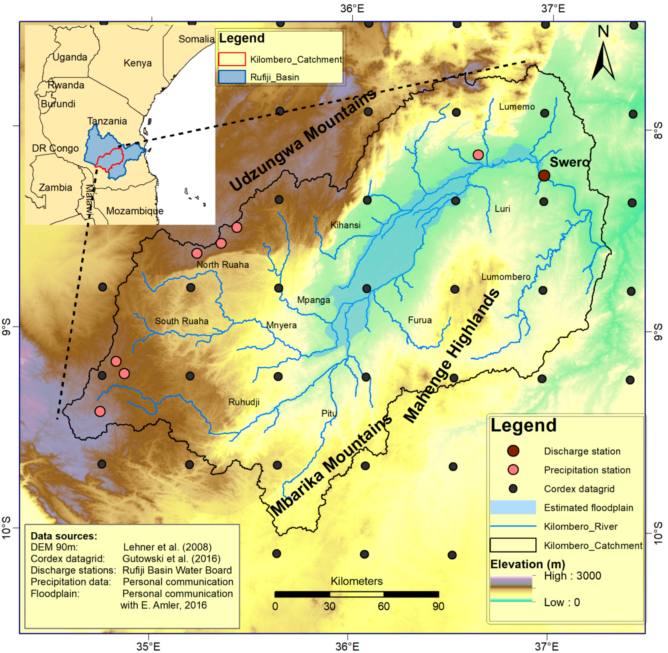
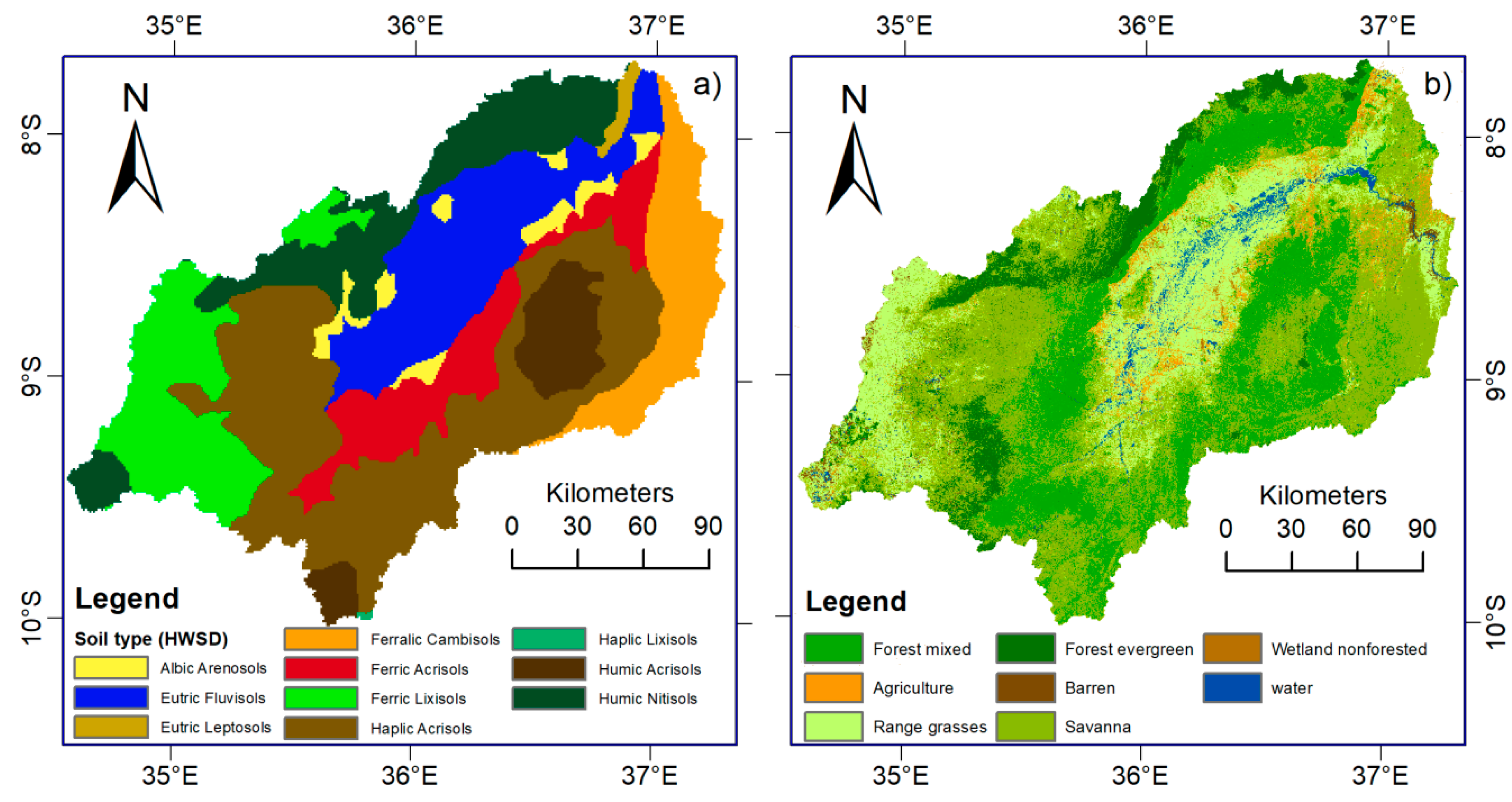
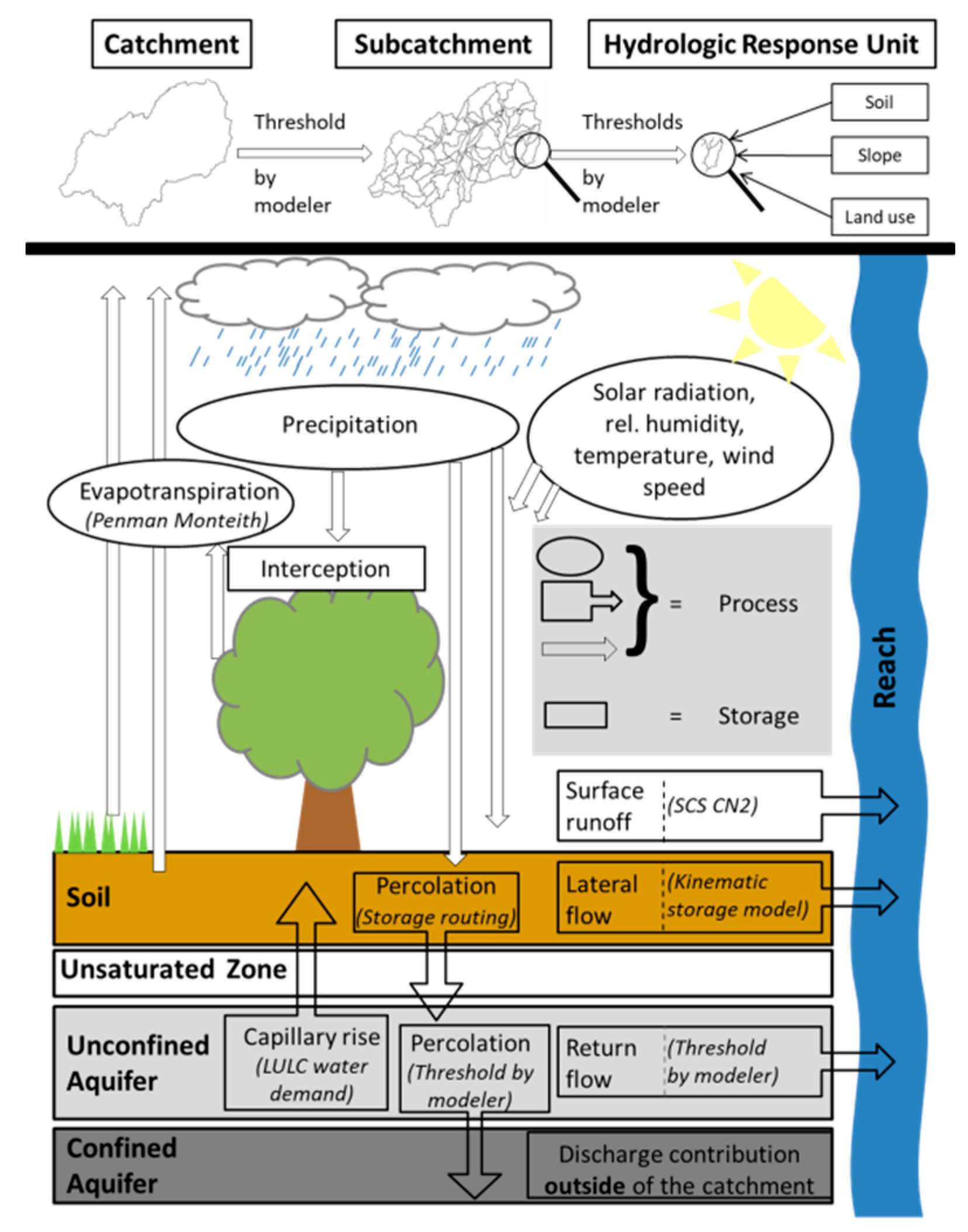
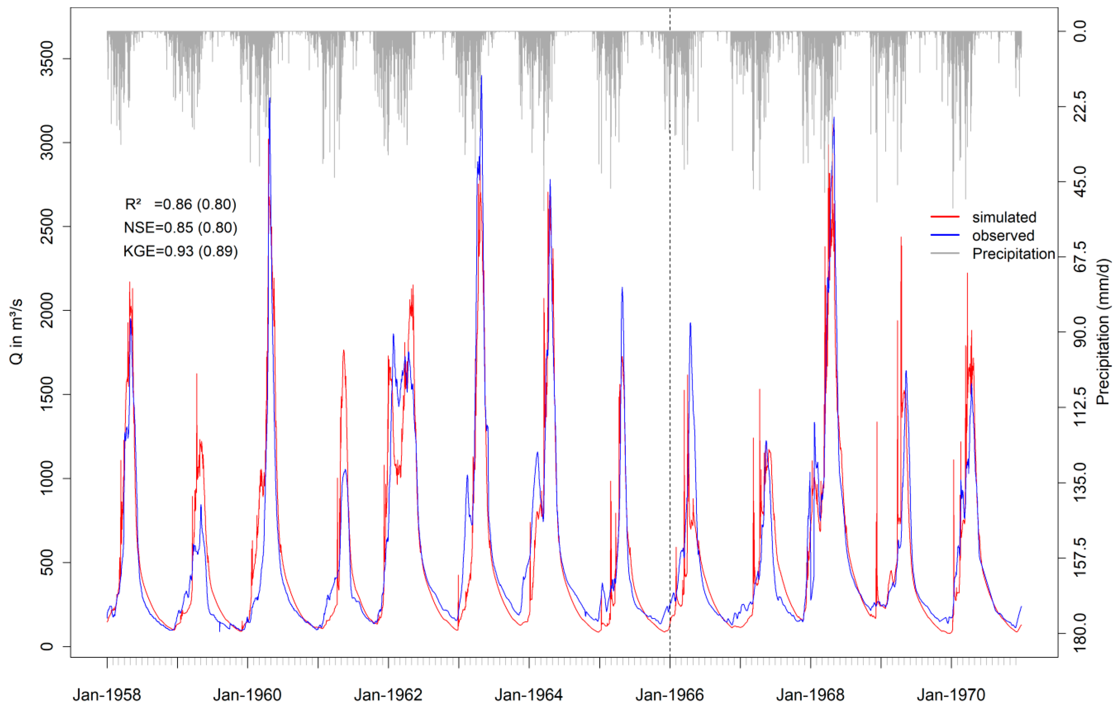
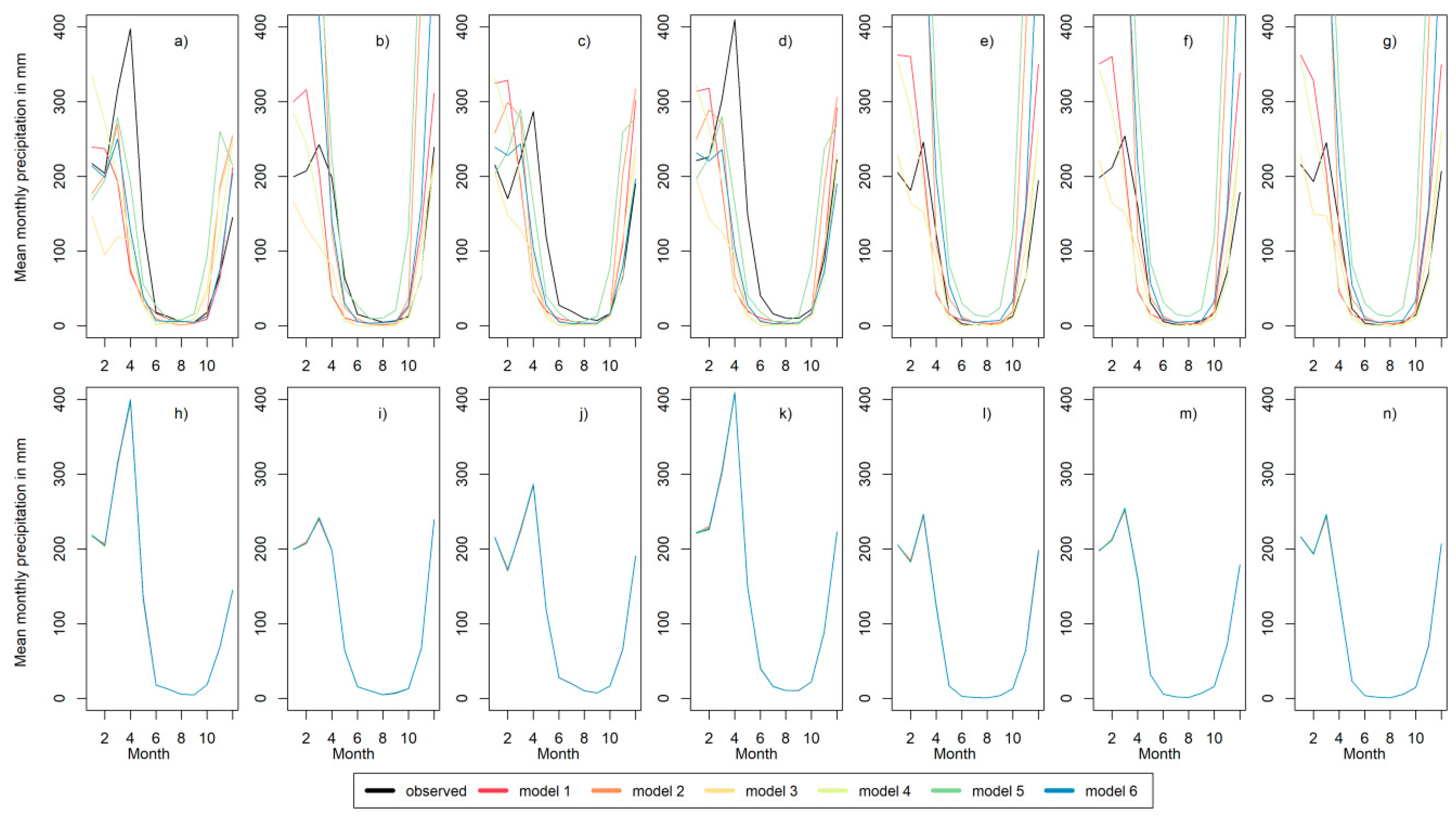
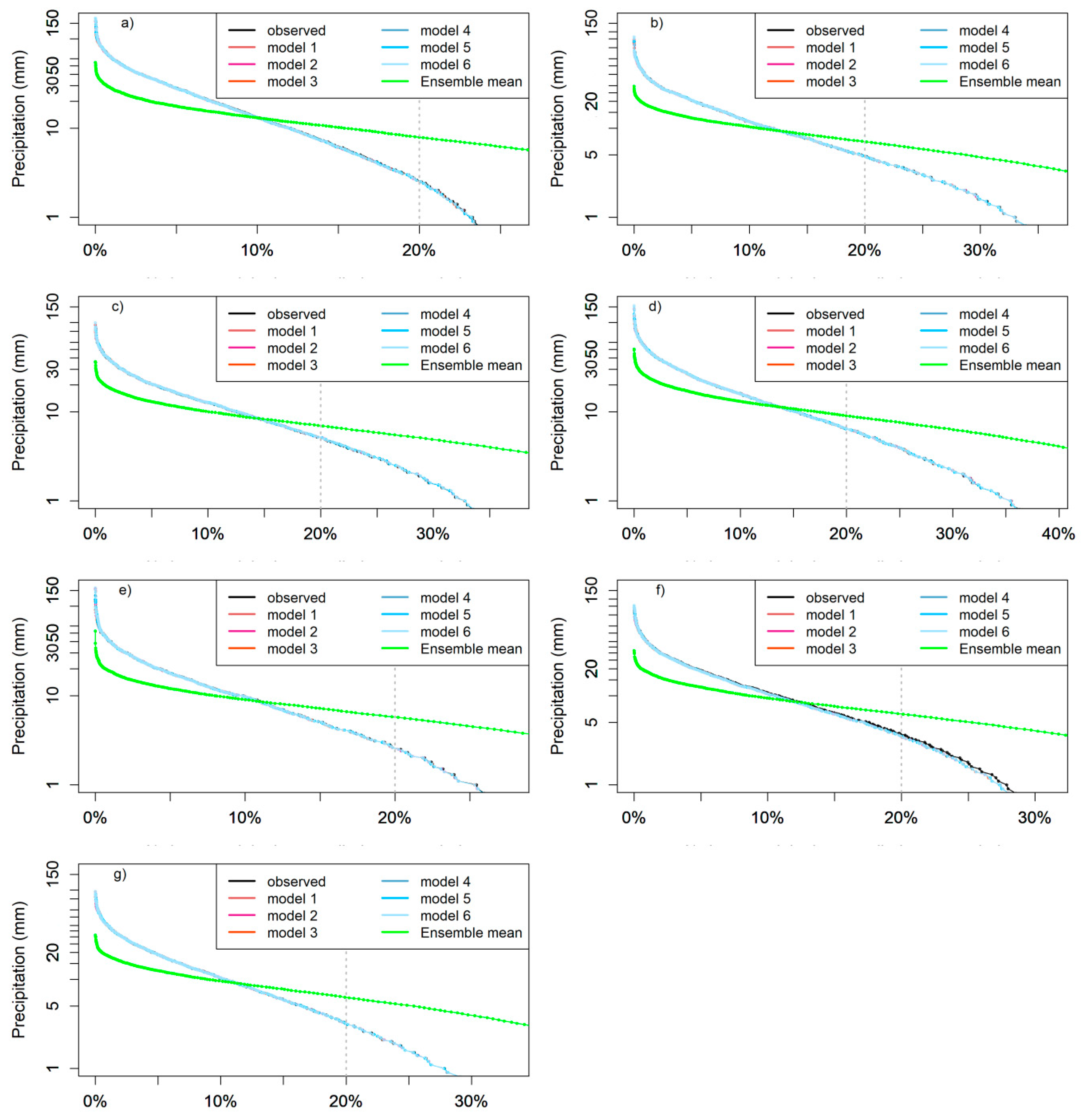
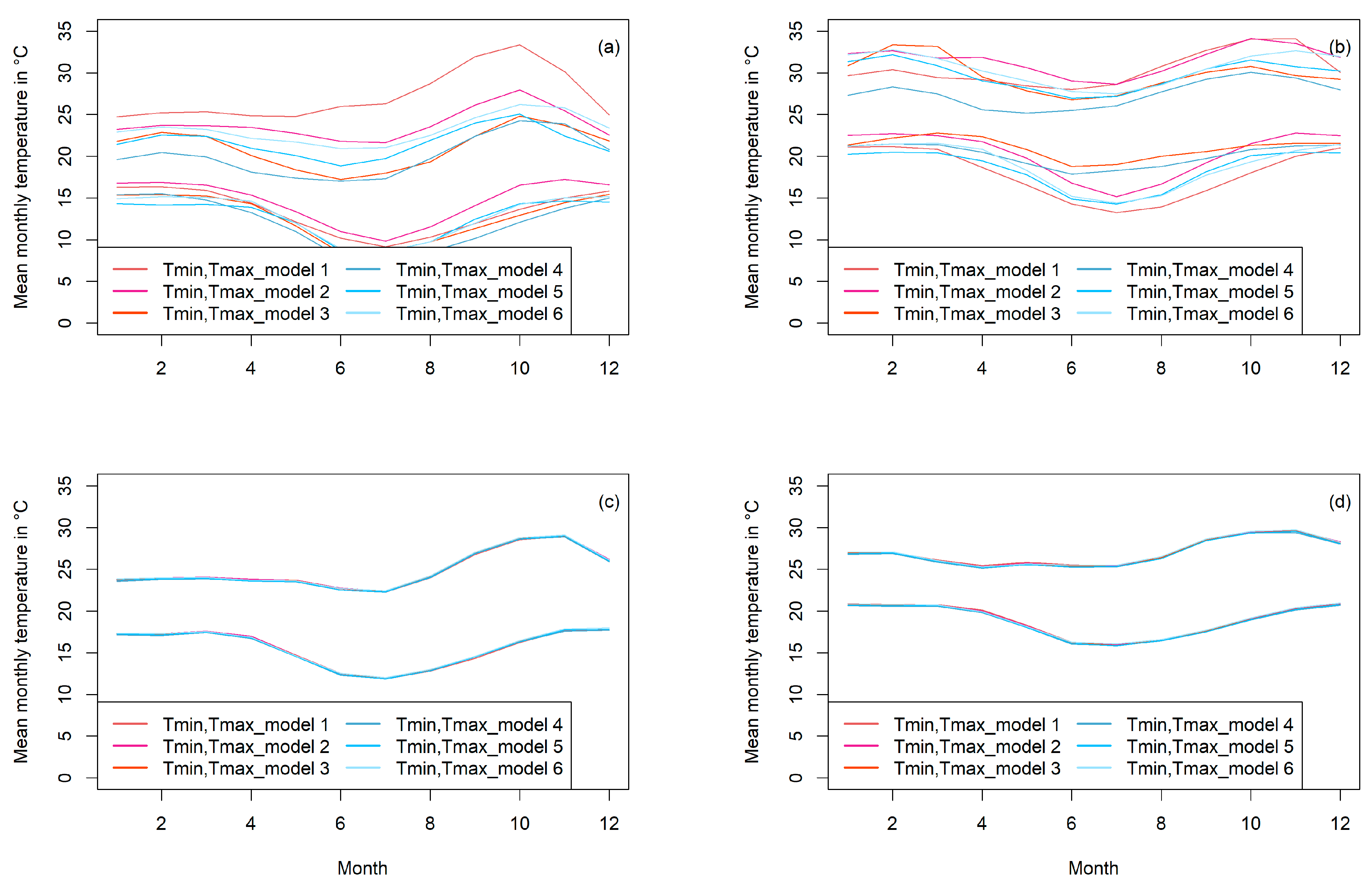
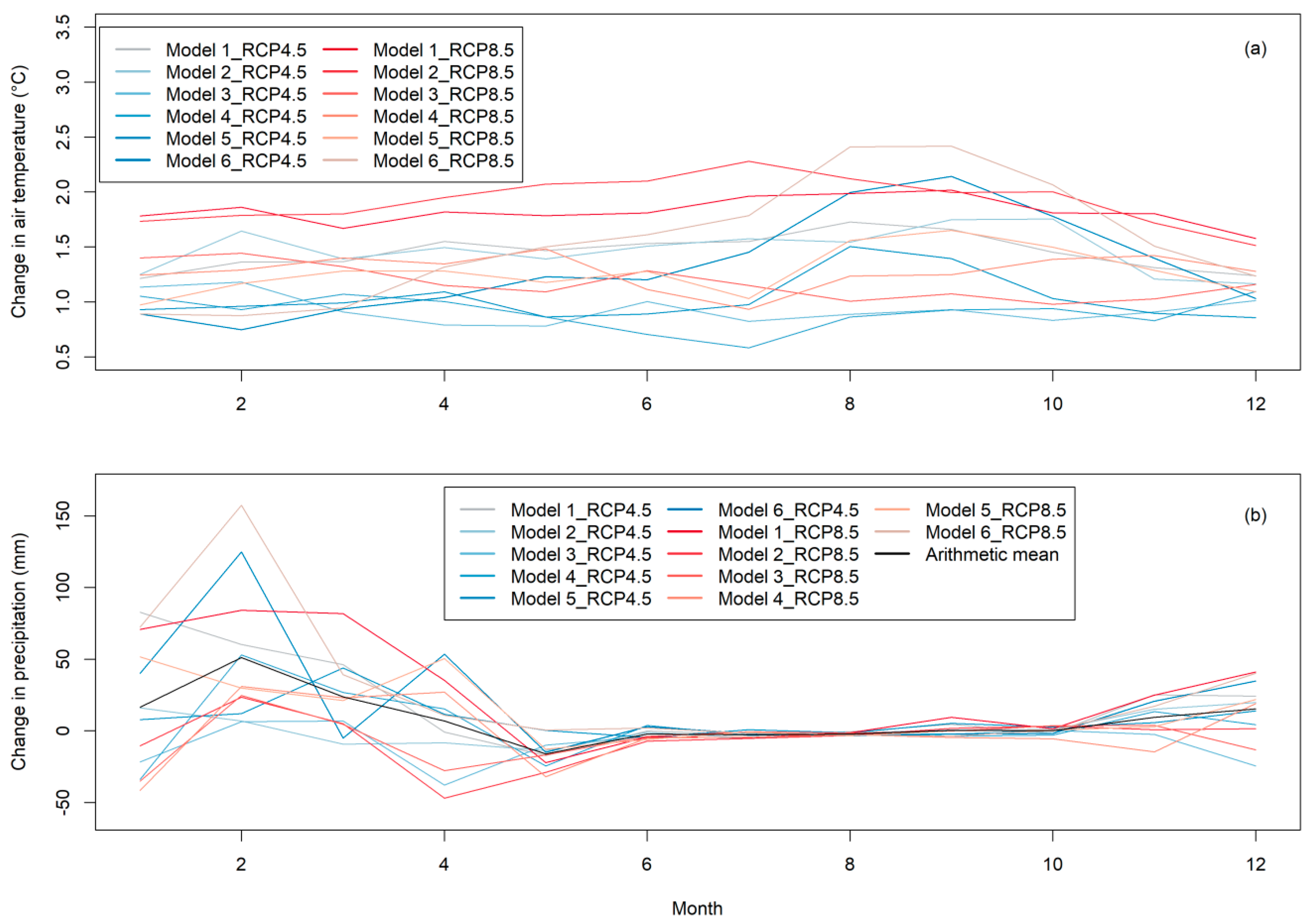
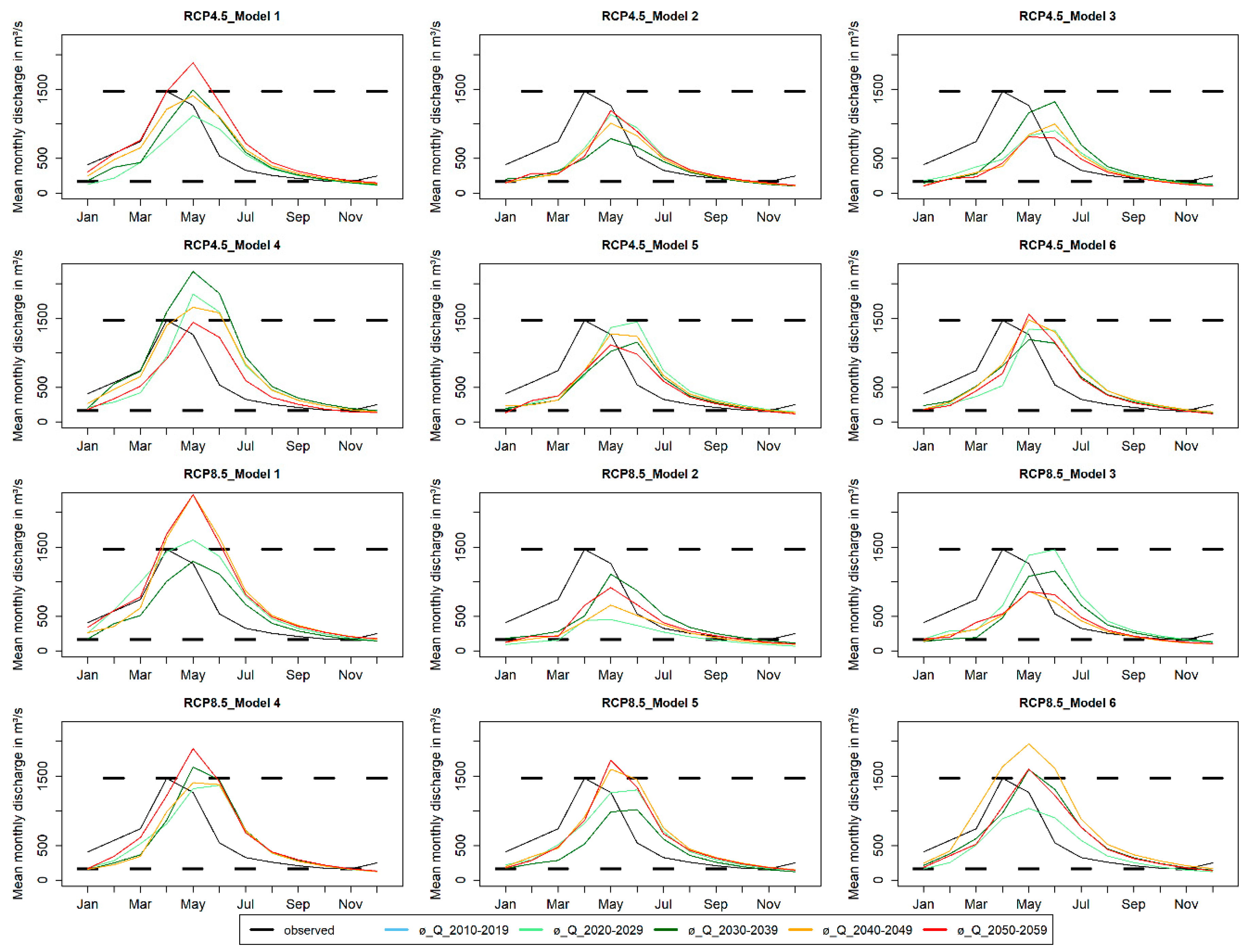
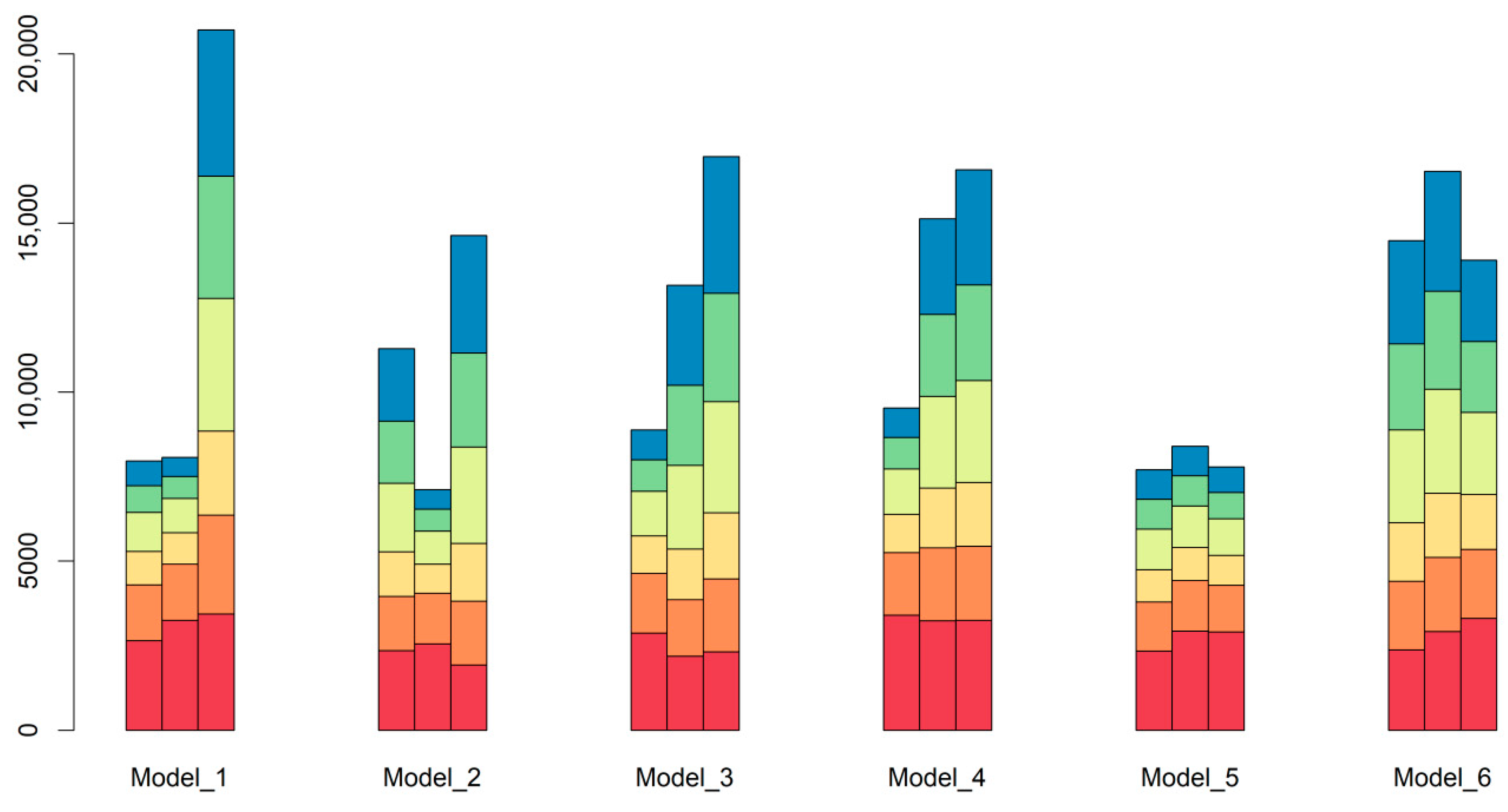
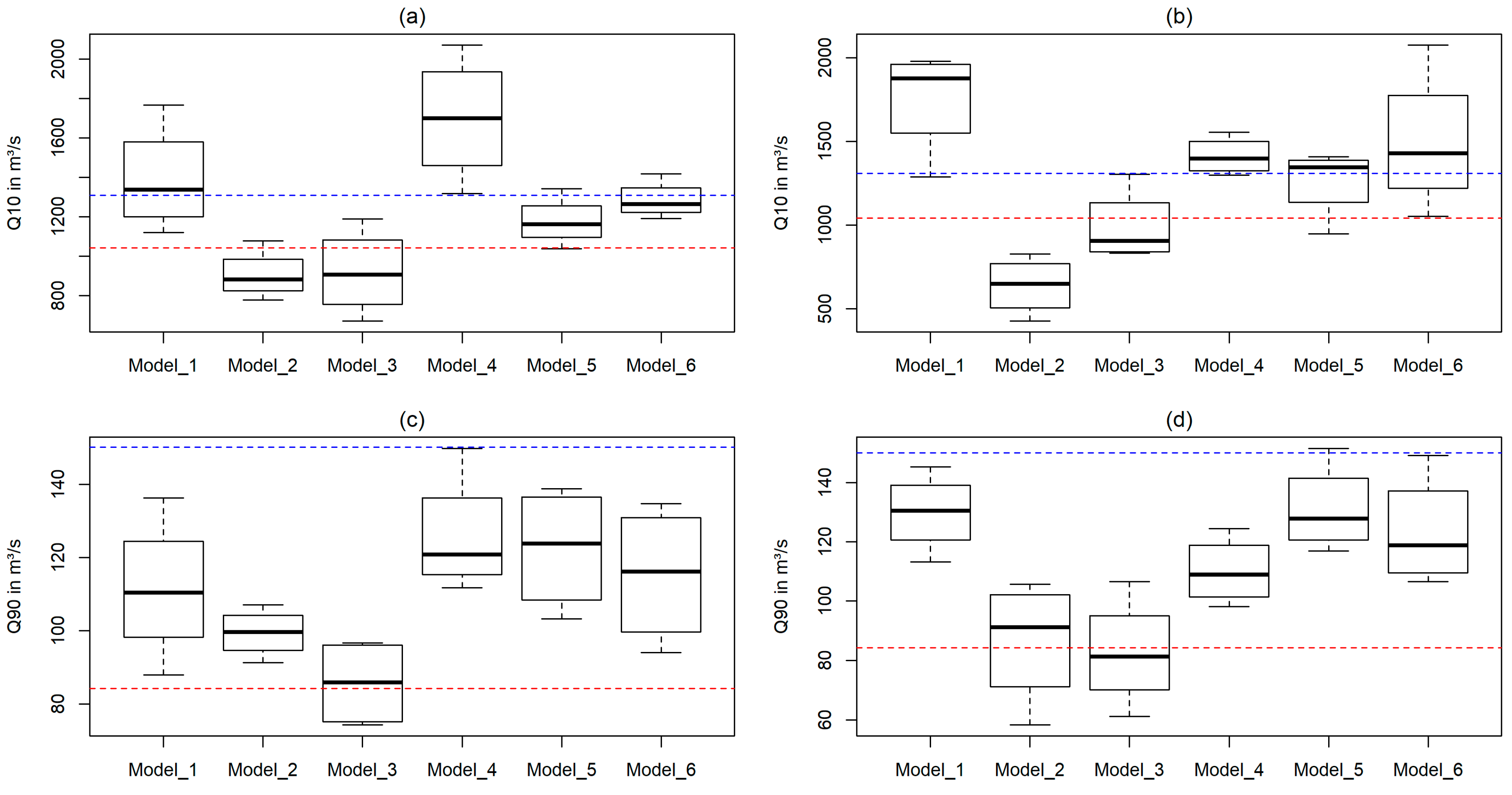
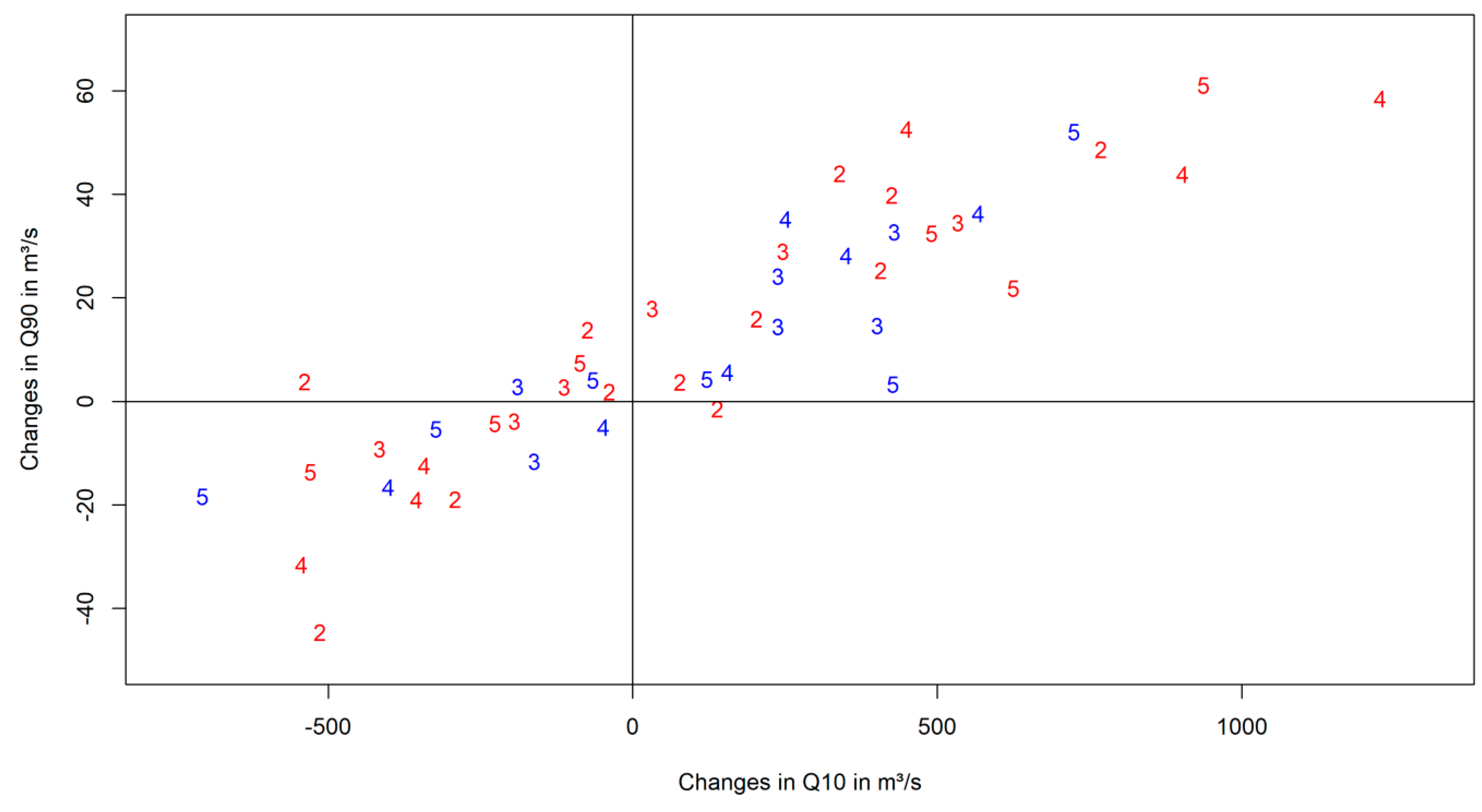
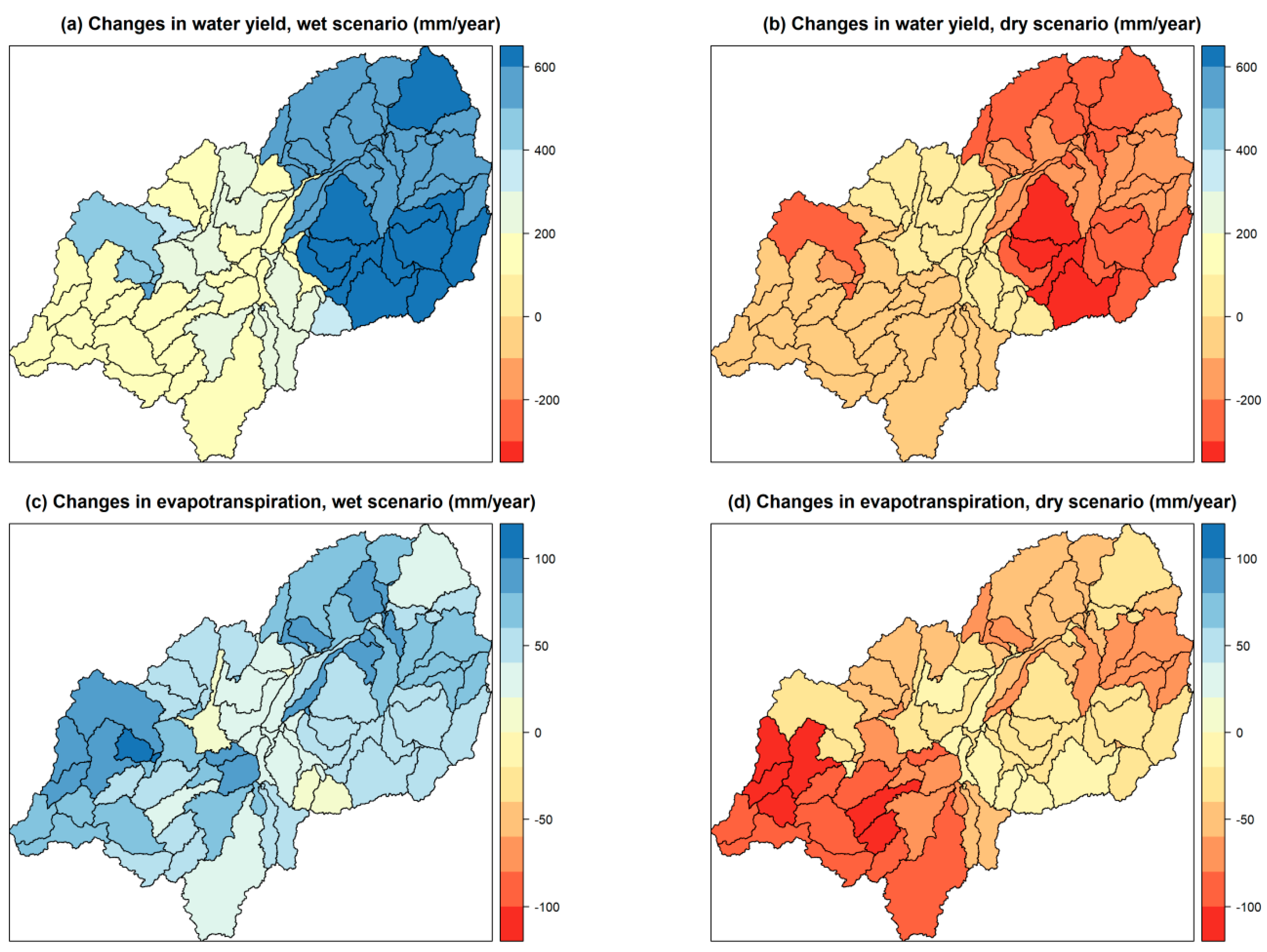
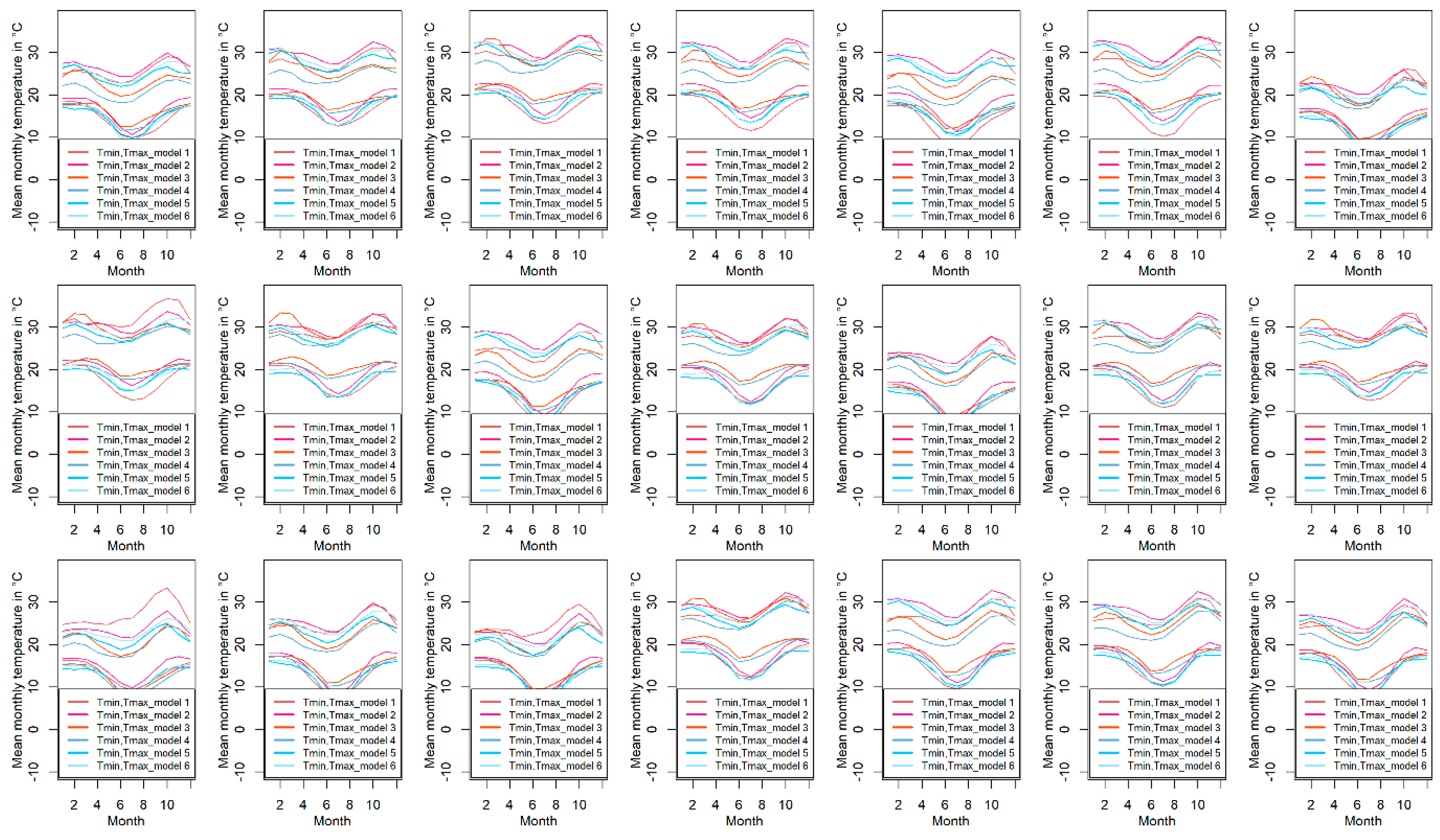
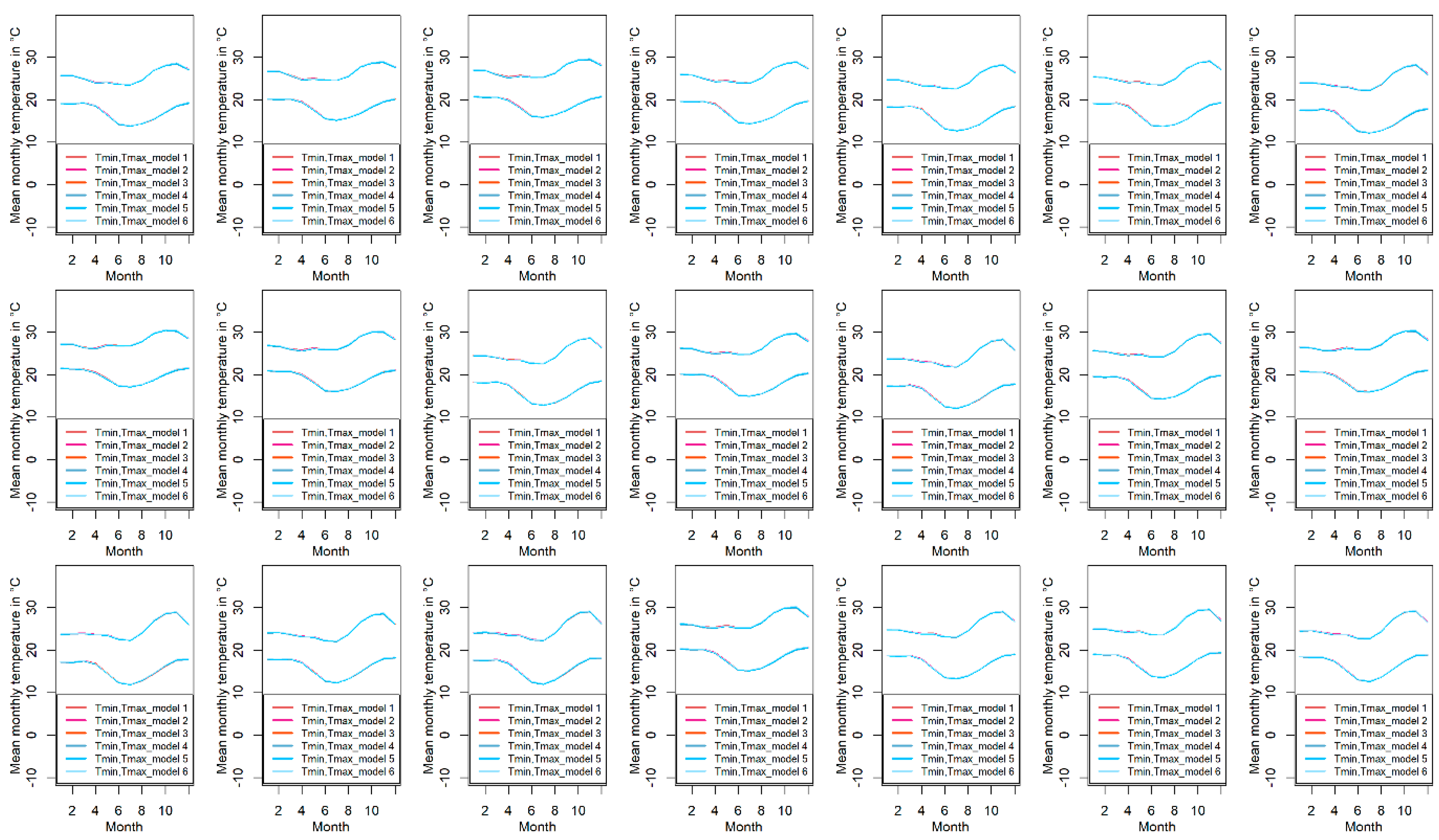
Table 1.
Overview of the applied datasets, their resolution, sources, and the required parameters in this study.
Table 1.
Overview of the applied datasets, their resolution, sources, and the required parameters in this study.
| Data Set | Resolution/Scale | Source | Required Parameters |
|---|---|---|---|
| Digital Elevation Model (DEM) | 90 m | Shuttle Radar Topography Mission (SRTM) [45] | Topographical data |
| Soil map | 1 km | Food and Agriculture Organization of the United Nations (FAO) [42] | Soil classes and physical properties |
| Land use map | 60 m (1970s) | Landsat pre-Collection Level-1 [46] | Land cover and use classes |
| Precipitation | Daily (1958–1970) | Personal communication: RBWB, University of Dar es Salaam (UDSM), Tanzania Meteorological Agency (TMA) | Measured precipitation |
| Climate | Daily/0.44° (1951–2060) | Coordinated Regional Downscaling Experiment (CORDEX) Africa [36] | Temperature, humidity, solar radiation, wind speed, precipitation |
| Discharge | Daily (1958–1970) | RBWB [47] | Discharge |
Table 2.
Overview of the Regional Climate Models (RCMs), their driving Global Climate Models (GCMs), and the assigned naming for the model combination within this study.
Table 2.
Overview of the Regional Climate Models (RCMs), their driving Global Climate Models (GCMs), and the assigned naming for the model combination within this study.
| GCM | RCM | Institution | URL | In This Study Referred to as |
|---|---|---|---|---|
| CanESM2 | CanRCM4_r2 | Canadian Centre for Climate Modelling and Analysis (CCCma) | http://climate-modelling.canada.ca/ | Model 1 |
| CanESM2 | RCA4_v1 | Rossby Centre, Swedish Meteorological and Hydrological Institute (SMHI) | https://esg-dn1.nsc.liu.se/ | Model 2 |
| CNRM-CM5 | CCLM4-8-17_v1 | Climate Limited-area Modelling Community (CLMcom) | https://esg-dn1.nsc.liu.se/ | Model 3 |
| EC-EARTH | CCLM4-8-17_v1 | Climate Limited-area Modelling Community (CLMcom) | https://esg-dn1.nsc.liu.se/ | Model 4 |
| EC-EARTH | RCA4_v1 | Rossby Centre, Swedish Meteorological and Hydrological Institute (SMHI) | https://esg-dn1.nsc.liu.se/ | Model 5 |
| MIROC5 | RCA4_v1 | Rossby Centre, Swedish Meteorological and Hydrological Institute (SMHI) | https://esg-dn1.nsc.liu.se/ | Model 6 |
Table 3.
Historical monthly average minimum (Tmin) and maximum temperature (Tmax) according to the bias-corrected RCM simulations (1979–2005). The given values represent the average of the monthly average Tmin and Tmax of all 21 utilized CORDEX Africa grids, respectively.
Table 3.
Historical monthly average minimum (Tmin) and maximum temperature (Tmax) according to the bias-corrected RCM simulations (1979–2005). The given values represent the average of the monthly average Tmin and Tmax of all 21 utilized CORDEX Africa grids, respectively.
| Jan | Feb | Mar | Apr | May | Jun | Jul | Aug | Sep | Oct | Nov | Dec | |
|---|---|---|---|---|---|---|---|---|---|---|---|---|
| Tmin | 19.2 | 19.1 | 19.2 | 18.5 | 16.4 | 14.3 | 14.0 | 14.6 | 15.9 | 17.7 | 19.0 | 19.5 |
| Tmax | 25.4 | 25.4 | 24.8 | 24.3 | 24.5 | 23.9 | 23.8 | 25.2 | 27.6 | 29.0 | 29.3 | 27.2 |
Table 4.
Historical annual average precipitation according to the bias-corrected RCM simulations (1951–2005) and the absolute and relative changes of precipitation, and related impacts on selected water balance components in SWAT simulations (2010–2060) according to the projections based on RCP4.5 and RCP8.5 scenarios. Numbers in parentheses represent the changes in percentage. For each parameter (except for the historical precipitation) and RCP scenario, the lowest and highest values according to the absolute changes are highlighted in red and blue, respectively. EM represents the ensemble mean, ET0 the actual evapotranspiration, ETp the potential evapotranspiration, SQ the surface runoff, and WYLD the overall water yield.
| Climate Model | Historical Precipitation (After bias-correction) | RCP Precipitation Changes in mm (%) | RCP ET0 Changes in mm (%) | RCP ETp Changes in mm (%) | RCP SQ Changes in mm (%) | RCP WYLD changes in mm (%) |
|---|---|---|---|---|---|---|
| Model 1 (RCP4.5) | 1338 | 195 | 39 | 73 | 23 | 124 |
| (14.5) | (4.4) | (4.7) | (40.2) | (28.7) | ||
| Model 2 (RCP4.5) | 1334 | 3 | −4 | 94 | 7 | −20 |
| (0.2) | (−0.4) | (5.3) | (12.0) | (−4.9) | ||
| Model 3 (RCP4.5) | 1311 | −109 | −10 | 66 | −12 | −103 |
| (−8.3) | (−1.4) | (5.1) | (−18.3) | (−19.8) | ||
| Model 4 (RCP4.5) | 1334 | 22 | −9 | 43 | 7 | 23 |
| (1.7) | (−1.3) | (3.8) | (10.8) | (3.6) | ||
| Model 5 (RCP4.5) | 1355 | 75 | 11 | 54 | 11 | 52 |
| (5.5) | (1.2) | (3.3) | (19.7) | (12.4) | ||
| Model 6 (RCP4.5) | 1345 | 218 | 14 | 81 | 25 | 163 |
| (16.2) | (1.5) | (4.5) | (42.1) | (42.1) | ||
| EM (RCP4.5) | 1335 | 68 | 0 | 70 | 2 | 46 |
| (5.1) | (0.0) | (5.0) | (25.4) | (8.5) | ||
| Model 1 (RCP8.5) | 1338 | 288 | 39 | 96 | 39 | 216 |
| (21.5) | (4.4) | (6.2) | (67.8) | (50.1) | ||
| Model 2 (RCP8.5) | 1334 | −83 | −16 | 136 | −5 | −91 |
| (−6.2) | (−1.8) | (7.8) | (−9.7) | (−22.5) | ||
| Model 3 (RCP8.5) | 1311 | −76 | 11 | 76 | −6 | −85 |
| (−5.8) | (1.5) | (5.9) | (−8.9) | (−16.3) | ||
| Model 4 (RCP8.5) | 1334 | −33 | −28 | 91 | 12 | −28 |
| (−2.4) | (−4.2) | (8.1) | (18.6) | (−4.4) | ||
| Model 5 (RCP8.5) | 1355 | 130 | 1 | 75 | 18 | 102 |
| (9.6) | (0.1) | (4.6) | (31.6) | (24.2) | ||
| Model 6 (RCP8.5) | 1345 | 302 | 25 | 81 | 38 | 239 |
| (22.5) | (2.7) | (4.5) | (63.4) | (61.6) | ||
| EM (RCP8.5) | 1335 | 88 | −2 | 101 | 3 | 60 |
| (6.6) | (−0.2) | (7.2) | (34.6) | (10.9) |
Table 5.
Arithmetic mean and standard deviation for the relative changes of the return levels across all six models and for the two RCP scenarios in comparison with the respective historical model runs. All values represent changes in %.
Table 5.
Arithmetic mean and standard deviation for the relative changes of the return levels across all six models and for the two RCP scenarios in comparison with the respective historical model runs. All values represent changes in %.
| Statistic Measure | 2-Year | 5-Year | 10-Year | 25-Year | 50-Year | 100-Year |
|---|---|---|---|---|---|---|
| Arithmetic mean | 8.60 | 9.58 | 13.19 | 20.47 | 27.89 | 37.19 |
| Standard deviation | 21.79 | 16.31 | 18.64 | 28.72 | 39.75 | 53.21 |
© 2019 by the authors. Licensee MDPI, Basel, Switzerland. This article is an open access article distributed under the terms and conditions of the Creative Commons Attribution (CC BY) license (http://creativecommons.org/licenses/by/4.0/).
Share and Cite
MDPI and ACS Style
Näschen, K.; Diekkrüger, B.; Leemhuis, C.; Seregina, L.S.; van der Linden, R. Impact of Climate Change on Water Resources in the Kilombero Catchment in Tanzania. Water 2019, 11, 859. https://0-doi-org.brum.beds.ac.uk/10.3390/w11040859
AMA Style
Näschen K, Diekkrüger B, Leemhuis C, Seregina LS, van der Linden R. Impact of Climate Change on Water Resources in the Kilombero Catchment in Tanzania. Water. 2019; 11(4):859. https://0-doi-org.brum.beds.ac.uk/10.3390/w11040859
Chicago/Turabian StyleNäschen, Kristian, Bernd Diekkrüger, Constanze Leemhuis, Larisa S. Seregina, and Roderick van der Linden. 2019. "Impact of Climate Change on Water Resources in the Kilombero Catchment in Tanzania" Water 11, no. 4: 859. https://0-doi-org.brum.beds.ac.uk/10.3390/w11040859
Note that from the first issue of 2016, this journal uses article numbers instead of page numbers. See further details here.