Article

Groundwater Level Prediction for the Arid Oasis of Northwest China Based on the Artificial Bee Colony Algorithm and a Back-propagation Neural Network with Double Hidden Layers

1
Key Laboratory of Subsurface Hydrology and Ecological Effects in Arid Region of Ministry of Education, School of Environmental Science and Engineering, Chang’an University, Xi’an 710054, China
2
Shaanxi Yining Construction Engineering Co. Ltd., Xi’an 710065, China
3
School of Science, Yanbian University, Yanji 133200, China
*
Author to whom correspondence should be addressed.
Submission received: 18 January 2019 / Revised: 21 April 2019 / Accepted: 22 April 2019 / Published: 24 April 2019
(This article belongs to the Section Water Resources Management, Policy and Governance)

Abstract

:
Groundwater is crucial for economic and agricultural development, particularly in arid areas where surface water resources are extremely scarce. The prediction of groundwater levels is essential for understanding groundwater dynamics and providing scientific guidance for the rational utilization of groundwater resources. A back propagation (BP) neural network based on the artificial bee colony (ABC) optimization algorithm was established in this study to accurately predict groundwater levels in the overexploited arid areas of Northwest China. Recharge, exploitation, rainfall, and evaporation were used as input factors, whereas groundwater level was used as the output factor. Results showed that the fitting accuracy, convergence rate, and stabilization of the ABC-BP model are better than those of the particle swarm optimization (PSO-BP), genetic algorithm (GA-BP), and BP models, thereby proving that the ABC-BP model can be a new method for predicting groundwater levels. The ABC-BP model with double hidden layers and a topology structure of 4-7-3-1, which overcame the overfitting problem, was developed to predict groundwater levels in Yaoba Oasis from 2019 to 2030. The prediction results of different mining regimes showed that the groundwater level in the study area will gradually decrease as exploitation quantity increases and then undergo a decline stage given the existing mining condition of 40 million m3/year. According to the simulation results under different scenarios, the most appropriate amount of groundwater exploitation should be maintained at 31 million m3/year to promote the sustainable development of groundwater resources in Yaoba Oasis.

1. Introduction

The social development and agricultural production of oases in arid regions rely on valuable groundwater resources. However, the long-term overexploitation of groundwater has continuously diminished groundwater levels, particularly in arid oases where surface water is extremely scarce and the ecological environment is fragile [1]. A decline in groundwater levels triggers a series of eco-environmental problems and seriously affects local agricultural production and economic development. These problems have been observed in typical oases, such as Yaoba [2], Minqin [3], and Keriya [4]. Eco-environmental crises caused by the unreasonable utilization of groundwater have been reported in Northwest China, particularly along the ancient Silk Road, which includes the Hexi Corridor [5,6], Tianshan Mountains [7], and the edge of the Tarim Basin [8]. The same problems have been observed in the desert oases of Australia, the United States, and Africa [9,10,11]. Groundwater level, which is an important indicator of groundwater balance, exhibits cyclical and random characteristics under the influences of climatic factors and human activities. Therefore, the accurate prediction of groundwater level is of great significance for the rational utilization of groundwater resources and the sustainable development of the social economy in arid areas.
A back-propagation (BP) neural network is a feed-forward and multi-layer network in an artificial neural network (ANN). Since its introduction, BP has been widely used in evaluation and prediction due to its strong connection ability and simple structure [12,13,14]. The accuracy of a BP neural network depends on the number of hidden layers. Kaveh and Servati (2001) [15] trained a BP neural network for the design of double-layer grids and observed an improvement in convergence speed and generalization capability. Neaupane and Achet (2004) [16] demonstrated that a BP neural network with one input layer, two hidden layers, and one output layer can deliver accurate results when used to predict slope movement. Métivier (2007) [17] concluded that a BP neural network with two hidden layers for forecasting stock prices is more accurate than a BP neural network with one, three, four, and five hidden layers. Haviluddin and Alfred (2014) [18] used a BP neural network with two hidden layers as a model to simulate network traffic usage and found that the method can obtain an appropriate mean square error (MSE). Akpinar et al. (2016) [19] accurately predicted natural gas consumption by using a BP model with two-hidden layers. However, a BP neural network suffers from defects. For example, this model is sensitive to random initial weights and thresholds, easily becomes trapped in local minima, and suffers from a slow convergence speed during training. Thus, the traditional BP neural network should be improved to develop a highly accurate model [20].
The artificial bee colony (ABC) algorithm is a swarm intelligence technology based on the simulated foraging behavior of honey-bees. The algorithm was proposed by Karaboga for real-parameter optimization in 2005 and then used to improve BP neural networks and solve local minima and instability issues in 2007 [21,22,23]. A BP neural network combined with the ABC algorithm has been increasingly applied in many fields, such as hydrological evaluation and prediction [24], demand forecasting [19], and system testing and optimization [25,26]. Many studies have proposed that the ABC algorithm exhibits a faster convergence rate and more accurate prediction compared with particle swarm optimization (PSO), genetic algorithm (GA), and ant colony optimization (ACO) [24,27]. In summary, the ABC algorithm, which is equipped with the various ability of the local search and global convergence, optimizes the initial weights and thresholds of a BP neural network with double hidden layers to achieve fast convergence performance, improve generalization capability, and avoid the tendency to fall into a network’s local minima [28,29,30].
In the current study, Yaoba Oasis was selected as the research area, and groundwater levels from 2019 to 2030 were predicted under different mining scenarios by developing and training an ABC-BP model with double hidden layers. This work aims to (i) study the future variation trends of groundwater levels and find the optimal exploitation quantity for the sustainable development of agriculture and (ii) provide scientific references for the rational utilization of groundwater resources and offer novel methodological concepts for similar studies in other arid oases.

2. Materials and Methods

2.1. Study Area

Yaoba Oasis is a typical desert oasis in Northwest China, which is the largest agricultural base of Alxa in the Inner Mongolia Autonomous Region. Yaoba Oasis lies west of Helan Mountain and east of Tengger Desert, extending between latitude 38°25′–38°36’ and longitude 105°34’–105°39’ (Figure 1a). The mean annual rainfall varies between 150 mm and 400 mm from west to east, and the average annual temperature is 8.29 °C. By contrast, the average annual evaporation ranges from 1400 mm in the east to 2400 mm in the west. The oasis exhibits a typical continental arid climate with several characteristics, namely, hot summer and cold winter, rare rainfall, and intense evaporation. Groundwater has become an important water resource for local agricultural production due to the scarce rainfall and extreme lack of surface water in Yaoba Oasis. The previous calculations of other researchers indicate that the total amount of groundwater recharge is maintained at 31 million m3/year, whereas the amount of groundwater exploitation is maintained at approximately 40 million m3/year in the study area [31]. Since the development of the oasis in the 1970s, overexploitation has been observed in the region [32]. Subsequently, groundwater levels have been dropping continuously with a cumulative depth of decline that exceeds 12 m [33]. Simultaneously, a series of eco-environmental problems has been triggered, including the contraction of adjacent lakes, intrusion of groundwater by salt-water, deterioration of groundwater quality, aggravation of soil salinization, degradation of surrounding grassland, and increase of land desertification; all of these problems seriously influence local economic development, agricultural production, and peoples livelihood [34].

2.2. Data Source and Process

Previous studies have reported that the major factors that influence groundwater levels in Yaoba Oasis include recharge, exploitation, rainfall, and evaporation, with exploitation as the most critical influencing factor that exerts the greatest effect [35]. The monitoring data of rainfall and exploitation are obtained from a local meteorological station, whereas the data of groundwater levels are derived from six wells of a dynamic monitoring network (Figure 1b). The physical magnitudes of the data between the four factors and groundwater levels are different. Thus, all the data are converted to monthly data, normalized within the range of [−1, 1], and restored to the actual predicted values in the prediction model output of the data.

2.3. Model Setup

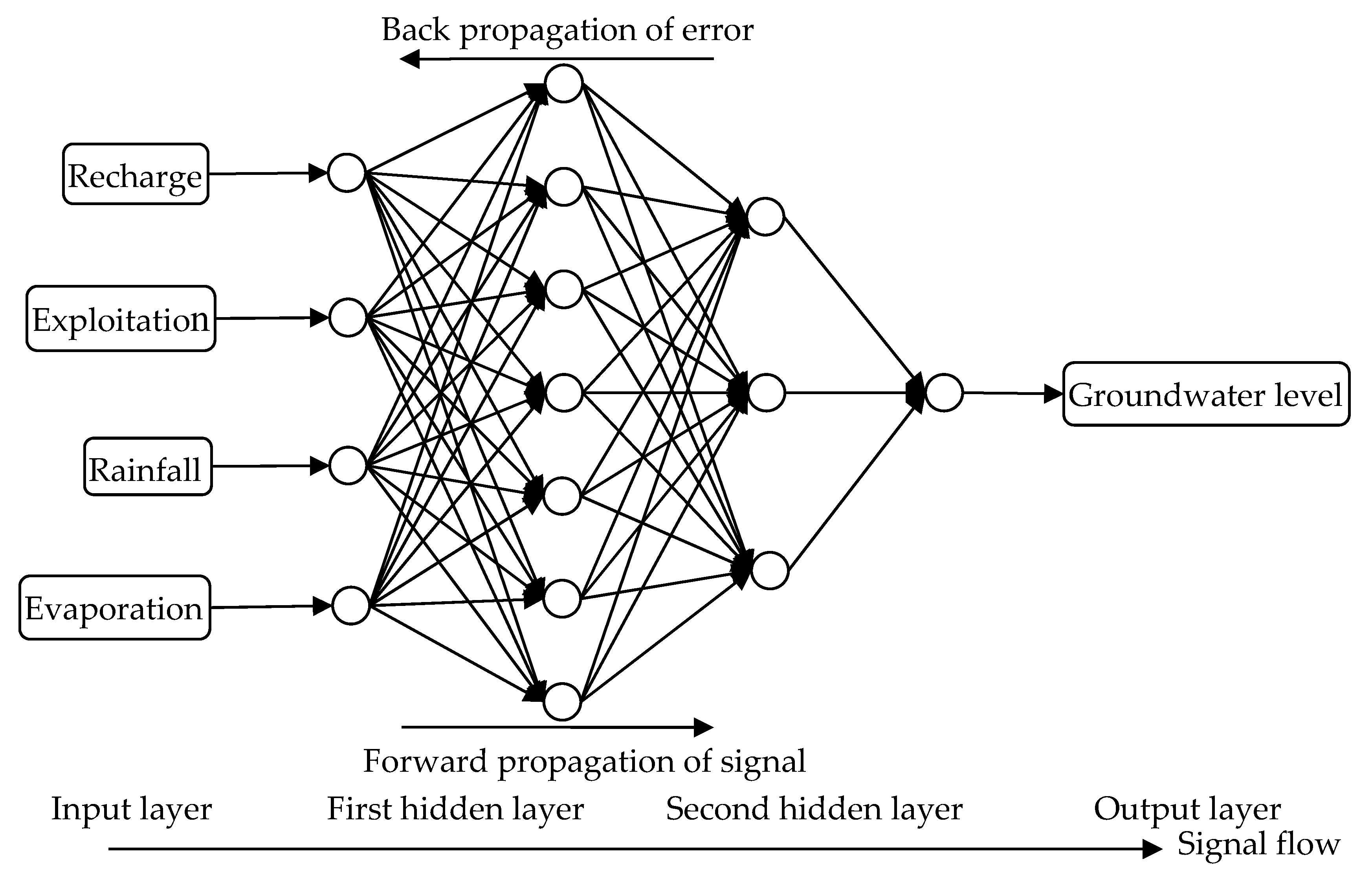
2.3.1. Topology of the BP Neural Network with Double Hidden Layers

Network topology, including the number of functional layers and the number of nodes in each layer, affects the generalization capability and prediction accuracy of the BP neural network [36]. The same network structure results in different outcomes for each training because the weights and thresholds are randomly initialized. A BP network for the design of double-layer grids was proven to improve generalization performance, overcome over-fitting, and deliver more accurate results than networks with one, three, four, and more hidden layers [17,37,38]. In the current work, a BP model with double hidden layers was developed to optimize network structure. The input, first hidden, second hidden, and output layers belonged to a four-layer working platform of the prediction model. The input layer was composed of four neuron nodes: recharge, exploitation, rainfall, and evaporation. The output layer consisted of one neuron node, namely, groundwater level.
The number of nodes in a hidden layer should be reasonably considered for under-fitting and over-fitting because these problems can decrease the generalization ability of a network. The error value of network training increases if the number of nodes in a hidden layer is either too few or too many. If the number of nodes is excessively few, then the network cannot fully determine the rule for the sample data, thereby resulting in the inability to establish a complex mapping relationship. In this case, the BP network exhibits under-fitting and the prediction error is large. By contrast, an excessive number of hidden nodes will not only make fitting the signal along with the noise easier but will also extend the learning and training times of the network, thereby resulting in the over-fitting phenomenon of the network and a large prediction error [39,40]. Selecting the number of hidden layer nodes is a highly complicated task. To accurately reflect the relationship between the input and the output, the principle states that fewer hidden layer nodes should be selected to make the network structure as simple as possible. In this work, the stepwise growing method of a network structure was adopted. In particular, only a few nodes were first set to train the network and test the learning error. Then, the number of nodes was gradually increased until the learning error was no longer considerably reduced. The optimal number of nodes in a hidden layer is commonly determined using Equation (1) [38,41,42].
m = n + l + a m 2 n + 1 m = log 2 n m = n l
where a represents a natural number within [1,10], and m, n, and l represent the nodes of the hidden, input, and output layers, respectively.
In the current study, the optimal numbers of nodes in the hidden layer were the range of [3, 9] calculated using multi-trials algorithms in accordance with the aforementioned formula. The error of the simulated and measured values in the network training firstly gradually decreased and then increased with the number of hidden layer neurons increased in Table 1. When the number of nodes in double hidden layer was set as 7-3, the training of the BP model reached the optimal level with the minimum error of 0.01. This result indicates the BP neural network with the above construction can meet the accuracy requirements the and overcome the overfitting problem. Therefore, seven and three were considered as a reasonable node for the first and second hidden layers, respectively. In the process of network training, the spatially weighted aggregation and excitation outputs of the input signal are provided by the seven neuron nodes in the first hidden layer, and the nonlinear mapping capability of the complex relationship between the input and the output is improved by the three neuron nodes in the second hidden layer [37]. Accordingly, the network topology of the BP model with double hidden layers was set to 4-7-3-1 in this work (Figure 2).
During forward propagation, a neural network receives the sample data and transmits the signal first to the input layer and then to the output layer after the hidden layer function. If the output results are consistent with the test samples, then network training is terminated. Otherwise, the weights and thresholds are repeatedly modified between each layer depending on the back propagation of the error. Network training is completed when the error of the total samples is less than the pre-set accuracy requirement [43].

2.3.2. Principle of the ABC Algorithm

The ABC algorithm has been widely applied to solving optimization problems due to its advantages of fast convergence and global search. The two core elements of the ABC algorithm are bees and food sources. The bees are grouped into three types: scout, employed, and onlooker bees. Scout bees are tasked to randomly search for the positions of food sources, whereas employed and onlooker bees are responsible for mining nectar. First, employed bees mark the size and quantity of a food source and release signals to share the path toward the food source with onlooker bees. Then, onlooker bees commit the food source to their memory and search the neighborhood for a better food source by adopting a greedy criterion. Lastly, if the same food source is mined for a certain period, then new scout bees find a new food source to replace the current one, thereby maximizing the amount of mined nectar [44]. In solving an optimization problem, the location of a food source represents the possible solution, whereas the amount of food source corresponds to the fitness of the solution [21]. Artificial bees search for global artificial food sources until an optimal solution is found. In summary, large quantities of food sources, equate to high-quality solutions.

2.3.3. ABC-BP Neural Network

A BP neural network is sensitive to random initial weights and thresholds; thus, this neural network can easily become trapped in local minima and exhibits slow convergence speed during training [20,22]. The ABC algorithm, which demonstrates local searching and global convergence abilities, is widely used in training BP neural networks. This algorithm can optimize randomly assigned weights and thresholds and effectively improve the convergence performance of a network [28,29,30]. In the current study, the ABC algorithm is adopted to train a BP neural network with double hidden layers, thereby constructing a new accurate prediction model. The modelling process of the ABC-BP model is presented as a flowchart in Figure 3. The specific steps are as follows.
(1) Construct the BP neural network
Input layer nodes n (n = 1, 2, …, Ninput), number of hidden layers (Nhidden), hidden layer nodes m (m = 1, 2, …, Nhidden), output layer nodes l (l = 1, 2, …, Noutput), training samples p (p = 1, 2, …, Ns), training algorithm, transfer functions among the hidden and output layers, and expected error are determined. Then, the objective function is established, and the results of this function should be optimized under the aforementioned conditions [45].
(2) Initialize the parameters of the ABC algorithm
The initial parameters of the ABC algorithm include the numbers of solutions (NS), bee colonies (NC), employed bees (Ne), and onlooker bees (NO); the maximum cycle number (MCN); and the limit value. The initial solution Xi (i = 1, …, NS) of the D-dimension vectors is a randomly generated number within the range of [−1, 1] [27]. NS, NC, Ne, NO, and D satisfy the following relationships:
N C = 2 N S = N e + N O N e = N O
D =   N i n p u t × N h i d d e n + N h i d d e n + N h i d d e n × N out p u t + N out p u t
where D is the number of optimization parameters; and Ninput, Nhidden, Noutput denote the number of neurons in the input, hidden, and output layers, respectively [24].
(3) The algorithm achieves the ideal state when fitness reaches “1”. The fitness value of each solution is calculated using Equation (4). An artificial employed bee finds a neighboring food source using Equation (5) and then makes a greedy selection to identify a better solution. If the fitness value of the new solution is superior to that of the old one, then the old solution is discarded and the new one is selected. Conversely, the update failure number of the old solution increases by “1” [46].
f ( X i ) = { 1 , M S E i = 0 1 M S E i + 1 , M S E i > 0
V i j = X i j + r a n d ( 1 , 1 ) ( X i j X k j )
where Vij is the value of the jth dimension of the ith solution, f(Xi) is the fitness value of Vij, i = {1, …, NS}, j = {1, 2, …, D}, k = {1, 2, …, NS}, and ki and k are randomly assigned. MSEi is the MSE of the ith solution.
(4) The probability value (Pi) of the ith solution is expressed as Equation (6). The artificial onlooker bee searches again (Equation (5)) for a new solution from neighboring solutions in accordance with Pi.
P i = f ( X i ) n = 1 N s f ( X n )
(5) If the update failure number of solutions exceeds the limit, then the solution is discarded. Subsequently, the employed bee becomes a scout bee that searches randomly for a new solution, which is generated from the calculation of Equation (7) and stored to replace the old solution [47].
X i = X m i n + r a n d ( 0 , 1 ) ( X m a x X m i n )
(6) Training is terminated when the cycle number reaches MCN. Otherwise, Step 3 is repeated. In this manner, the initial weights and thresholds of the BP neural network are represented by the optimal solutions of the ABC algorithm. The cycle number is defined using Equation (8).
c y c l e = c y c l e + 1
(7) The ABC-BP model with double hidden layers is trained and tested with the sample data to achieve groundwater level prediction.

3. Results and Discussion

3.1. Model Validation

3.1.1. Initialization of Model Parameters

Considering the combination of the ABC algorithm and the BP neural network with double hidden layers, the ANN function of MATLAB 2014a was used to create and train the ABC-BP model through programming. The training algorithm of the BP neural network and the transfer functions of the hidden and output layers exert considerable influences on the accuracy of the prediction model [38]. Levenberg-Marquardt (“trainlm”), a BP algorithm and training function of the BP neural network, can effectively shorten the convergence time and improve the convergence performance of a network compared with other training functions, such as “trainscg”, “traincgp”, “trainrp”, and “traingdx” [48,49,50]. The “sigmoid”-type transfer functions of the BP neural network with multiple hidden layers are commonly used between hidden layers, including “tansig” and “logsig”, and the linear transfer function “purelin” is typically used between the neurons of the output layer [49]. Many combined allocations exist among three transfer functions with “tansig”, “logsig”, and “purelin”. The BP model with double hidden layers can overcome the overfitting problem and achieve the optimal prediction effect when the algorithm “trainlm” was selected as the training function, the function “tansig” was selected as the transfer function from the input layer to the first hidden layer, the function “logsig” was selected as the transfer function from the first hidden layer to the second hidden layer, and the function “purelin” was selected as the activation function from the second hidden layer to the output layer [51,52]. The momentum factor, learning rate, maximum number of trainings, and expected error were set as 0.3, 0.01, 240, and 0.01, respectively. The monthly average recharge, exploitation, rainfall, and evaporation data from January 2010 to December 2016 were used as input data. The monthly mean groundwater level data from January 2010 to December 2016 were used as training samples. The monthly average groundwater level data from January 2017 to December 2018 were used as test samples. Evidently, a large bee colony is equivalent to the identification of superior solutions. Nevertheless, this procedure increases the computational complexity of the algorithm. In the simulation test, the initial numbers of employed bees (Ne) and onlooker bees (NO) were set as 100, the number of bee colonies (NC) was 200, the MCN was 150, and the limit value was 100, which should be greater than the D-dimension of each solution.

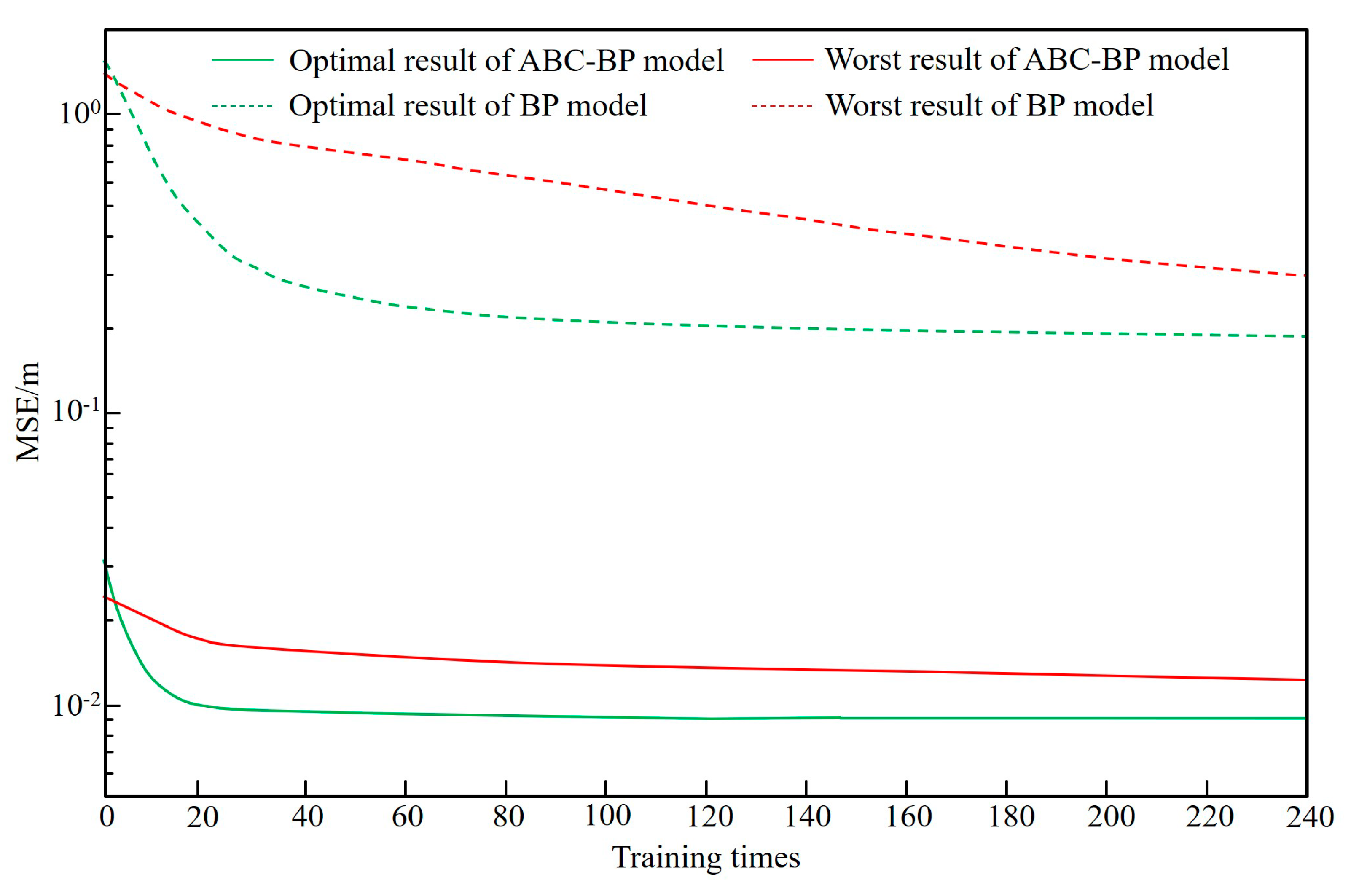
3.1.2. Model Training

After the initial parameters were set, the ABC-BP model trained the input data, tested the sample data several times, and ended the training upon achieving the optimal effect. The analysis result of the relationship between the fitness value and the cycle number in the training period indicated that the fitness value rapidly increased with the iteration times during the early stages (Figure 4). This finding demonstrated that the obtained solution became increasingly optimized. Fitness gradually stabilized at a constant value after a series of cycles. The result indicated that the model completely converged when the cycle number reached 150. The training results showed that the convergence rate of the BP neural network was improved by the ABC algorithm in terms of solving optimization problem.
As network training was completed, the initial weights and thresholds of the BP neural network were obtained using the ABC algorithm. The weight W1 and threshold B1 of the input layer to the first hidden layer are respectively given as follows:
W 1 = [ 1.831 1.935 0.589 2.914 1.606 2.224 0.485 1.422 0.231 0.422 - 3.011 2.082 2.119 1.343 0.715 2.321 0.977 1.683 - 2.318 1.656 2.768 1.705 1.475 1.849 2.604 0.963 0.406 2.362 ] B 1 = [ 2.271 0.554 1.395 3.604 1.792 0.965 1.416 ]
The weight W2 and threshold B2 of the first hidden layer to the second hidden layer are given as follows:
W 2 = [ 0.856 1.353 1.519 0.834 1.317 0.362 0.051 1.911 1.012 0.392 1.716 1.128 1.629 2.375 1.245 0.076 0.623 3.286 0.209 0.734 0.246 2.504 0.621 1.829 1.164 0.843 0.077 1.207 ] B 2 = [ 0.609 1.476 0.921 2.315 ]
The weight W3 and threshold B3 of the second hidden layer to the output layer are given as follows:
W 3 = [ 1.391    0.105    0.647    2.526 ] B 3 = [ 1.027 ]

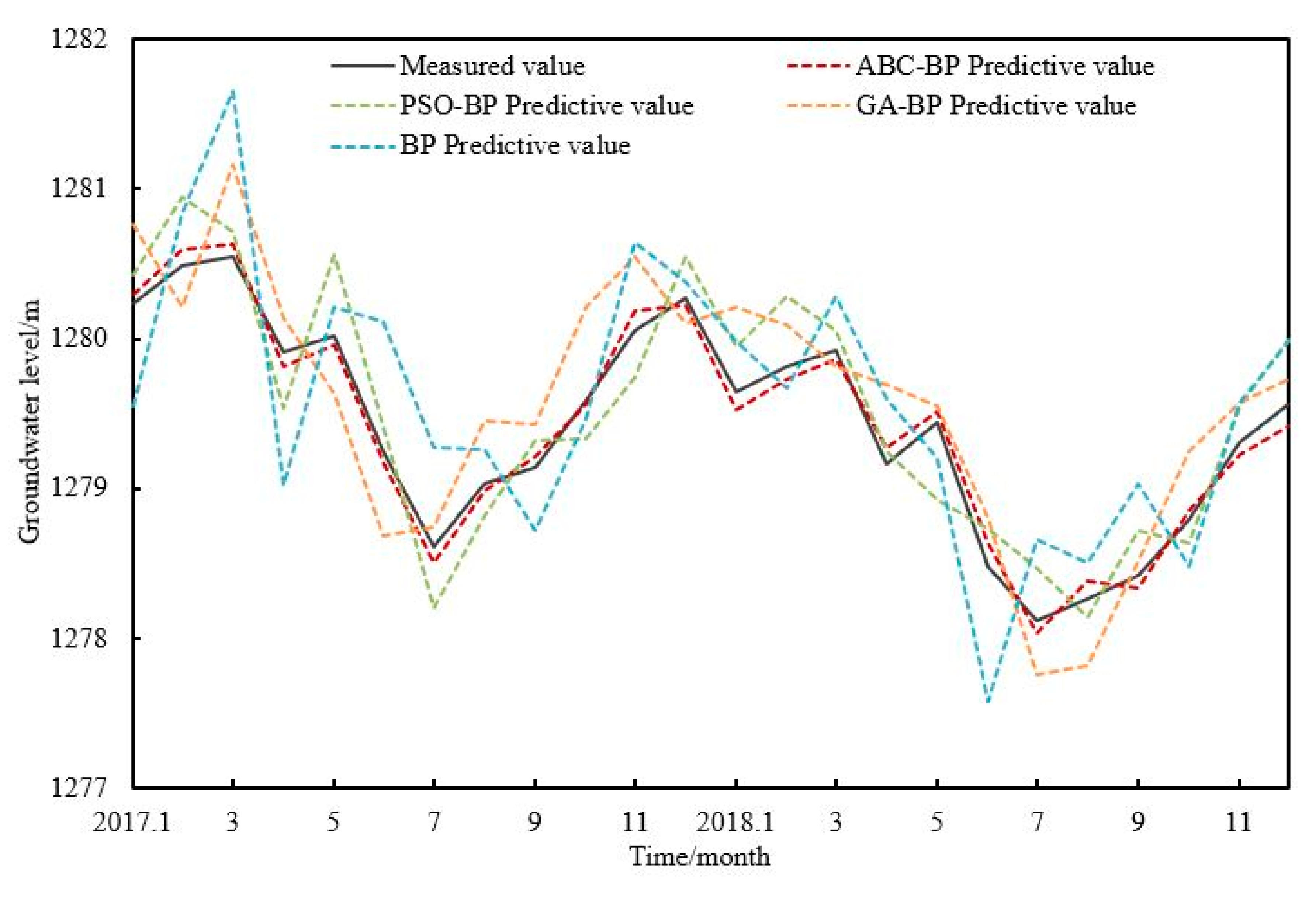
3.1.3. Comparison of ABC-BP, PSO-BP, GA-BP and BP Models

The ABC-BP and BP models were trained, and the groundwater level data were simulated several times to verify the feasibility and superiority of the ABC-BP prediction model. The optimal and worst training results of the two models were selected for comparative analysis. Figure 5 clearly shows that the relative error (RE) in the worst training of the ABC-BP model was slightly lower than that in the optimal training of the BP model. Moreover, the RE in the optimal training of the ABC-BP model was maintained at a low value of approximately 0.007. Hence, the accuracy of the ABC-BP model was higher than that of the BP model. In addition, the results of the ABC-BP model remained consistent after several runs, which demonstrated that this model considerably improved prediction stability. The multiple training results for groundwater levels obtained using the BP model differed from those obtained using the ABC-BP model. The iteration times and final RE of each training varied due to the randomness of the weights and thresholds in the BP model. Thus, the prediction results of the traditional BP model were unreliable.
As shown in Figure 6, the logarithmic variation curves of the MSE values in the optimal and worst training of the ABC-BP model were always lower than those of the BP model throughout the entire test process. The finding implied that the accuracy of the ABC-BP model was higher than that of the BP model. Furthermore, the ABC-BP model can obtain a small MSE of 0.01 after 20 training times and reached the predetermined error accuracy through a few cycles [24]. By contrast, the optimal and worst curves of the BP model demonstrated slow convergence rate, thereby verifying that the ABC-BP model can considerably improve prediction accuracy and ensure a fast convergence rate.
In addition, the predicted and error values of the ABC-BP model were compared with those of the PSO-BP, GA-BP, and BP models under the optimal training conditions in this work. The fitting results of groundwater levels in the monitoring well ZB-03, as shown in Table 2 and Figure 7, were used as examples. All the absolute error (AE) values remained within 0.16 when the network training of the ABC-BP model ran optimally, and the change range of AE and RE were minimal. Such results indicated that the prediction accuracy of the ABC-BP model was high and met simulation accuracy requirement. However, the AE values were maintained at approximately 0.46 in the optimal training of the BP model, and serious AE errors that exceeded 1.1 occurred during individual training. This result failed to meet the accuracy requirement for groundwater level prediction. The AE values of the PSO-BP and GA-BP models in the optimal training were kept at approximately 0.28 and 0.35, respectively. Although the predicted values were acceptable in most cases for the PSO-BP and GA-BP models, the AE values of the two models were higher than those of the ABC-BP model. As a result, the ABC-BP model comparatively performed best in the prediction effect of groundwater levels, and the simulated values of groundwater levels were closest to the true values. PSO-BP ranked second, followed by GA-BP, and the BP model demonstrated the worst performance.
In addition to AE and RE, four error representations were used to compare several algorithms to better illustrate the filtering effects of the four models and highlight the superiority of the ABC algorithm. The coefficient of determination (R2) represents the degree of relevant correlation between the measured and predicted values. The closer R2 is to “1”, the higher the correlation is. Conversely, the closer R2 is to “0”, the lower the correlation is [45]. As listed in Table 3, the R2 values of the ABC-BP, PSO-BP, GA-BP, and BP models were 0.983, 0.864, 0.826, and 0.653, respectively. It illustrated that the ABC-BP model matched better than the other three models. Moreover, the other three errors of the ABC-BP model were smaller than those of the three other models. The root MSE (RMSE) and maximum RE (REmax) of the PSO algorithm were smaller than those of the GA algorithm, whereas their mean AE (MAE) were similar. The RMSE, MAE, and REmax of the BP model were the highest, thereby indicating that the traditional BP neural network provided the worst prediction accuracy. The comparative analysis results of the four models were found that the ABC-BP model exhibited the better prediction accuracy and optimization performance, followed by the PSO-BP, GA-BP, and BP models in turn. Thus, the ABC algorithm was selected to optimize the BP neural network to further simulate the groundwater levels of the six wells in the next part of this work.
According to Figure 8, the measured values of the six wells were in the recovery phase from January 2017 to March 2017, October 2017 to March 2018, and October 2018 to December 2018 which was in the non-irrigation period when minimal mining activities were conducted. As summer and autumn irrigation began, exploitation amount dramatically increased, and thus, groundwater level gradually dropped from April 2017 to September 2017 and April 2018 to September 2018. The predicted values of the six monitoring wells obtained using the ABC-BP model fitted the measured values well. This result further illustrated that the ABC-BP model can effectively express the nonlinear relationship between the four aforementioned influencing factors and groundwater level. The ABC-BP model can also accurately simulate the trend of groundwater levels. In summary, the ABC-BP model can be used as an effective tool for forecasting the future groundwater levels of Yaoba Oasis.

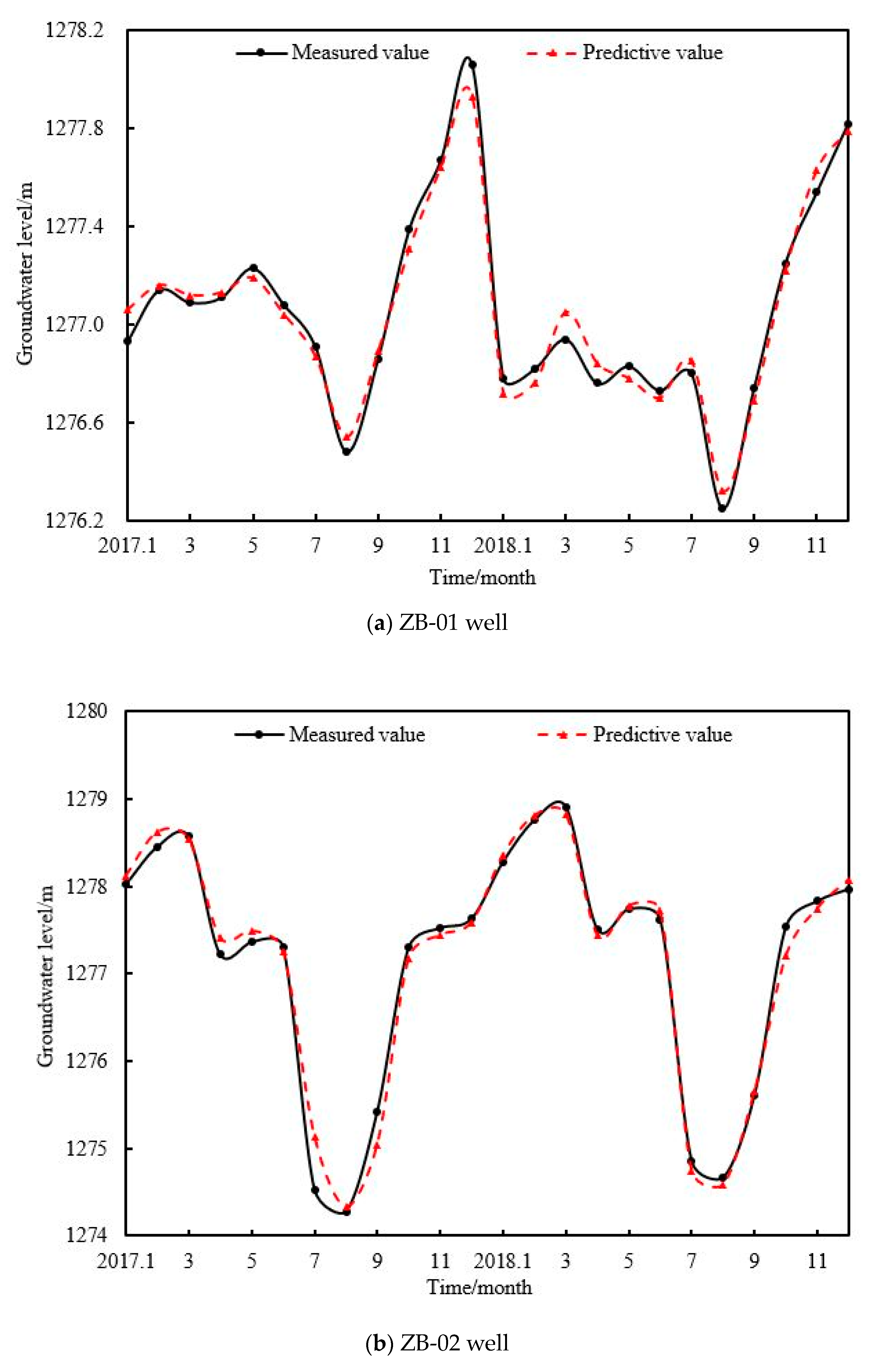
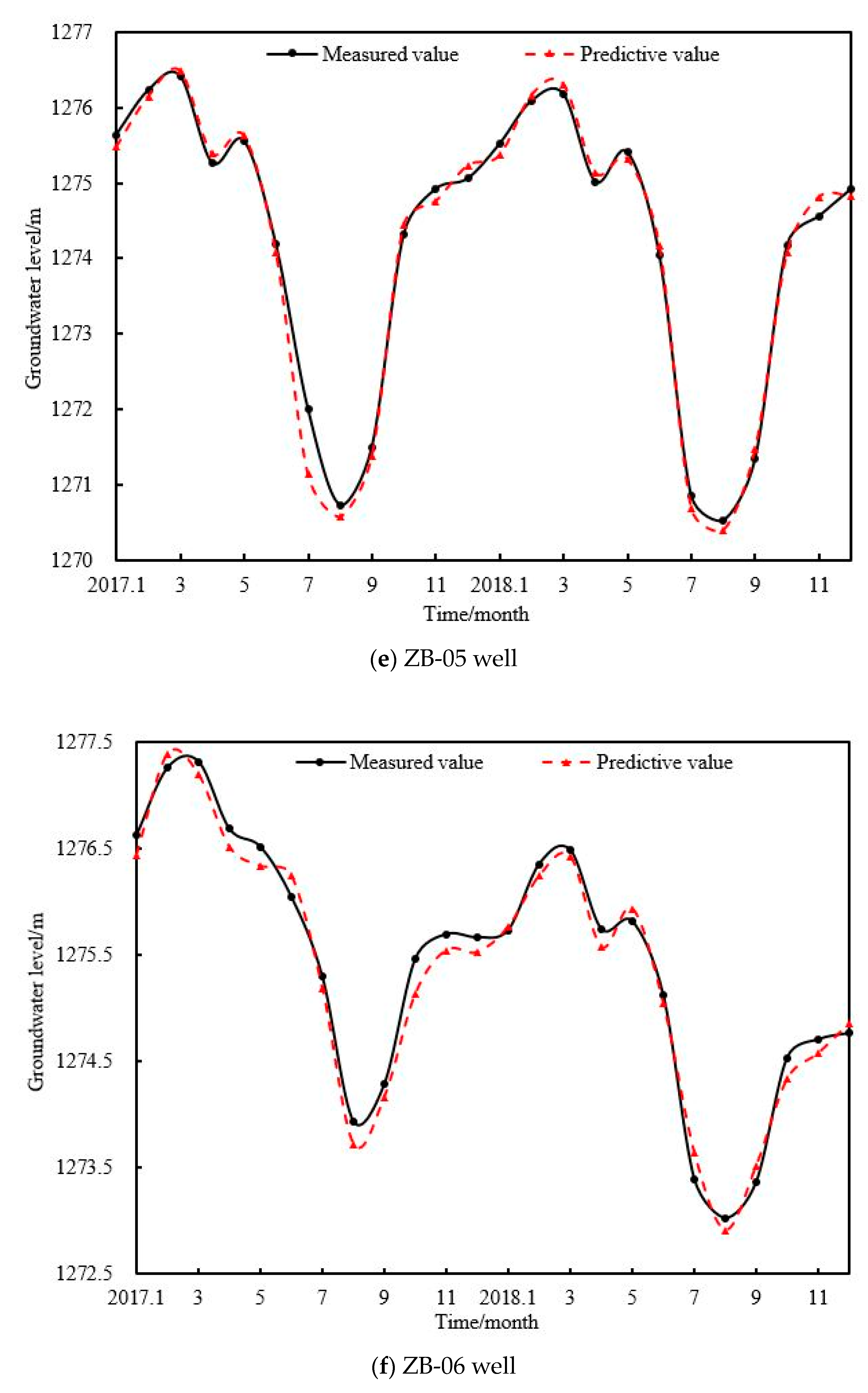
3.2. Groundwater Level Prediction under the Existing Mining Scenario

In this study, the trained ABC-BP model with double hidden layers was applied to predict the monthly groundwater levels of six monitoring wells. The prediction results of the six wells from 2019 to 2030 under the existing mining scenario are provided in Table 4 and Figure 9. As seen from Table 4, the groundwater level of Yaoba Oasis under the exploitation of 40 million m3/year will gradually drop with a total range of 1.31 m to 5.50 m and a descending rate of 0.11–0.46 m/a. The groundwater level of ZB-03 will gradually drop from 1279.51 m in 2019 to 1274.01 m in 2030, which will be the largest dropping occurring in the central and southern areas. The analysis result of the simulated values shows that the decreased amplitude of groundwater level will be 0.71–1.68 m from 2019 to 2024 with a decline rate of 0.12–0.28 m/a. The decline of groundwater level from 2025 to 2030 will be 0.59–3.82 m, and the drop speed will be 0.10–0.64 m/a. In summary, the cumulative decline range of groundwater level from 2019 to 2030 will be large given the current mining mode.
Figure 9 clearly illustrates that the six monitoring wells exhibited a gradual declining tendency. The analysis of the local situation indicated that the amount of groundwater exploitation at present is maintained at approximately 40 million m3/year, which already exceeds the total recharge amount of 31 million m3/year in the study area. Under the existing mining condition, the exploitation quantity is greater than the locally allowed mining level. Consequently, the groundwater levels will drop considerably in the future and may cause substantial damage to groundwater circulation and the eco-environment. With the future development of the social economy, industry, and agriculture, groundwater demand can increase considerably. Hence, the decline rate and amplitude of groundwater level will be larger than the predicted value.

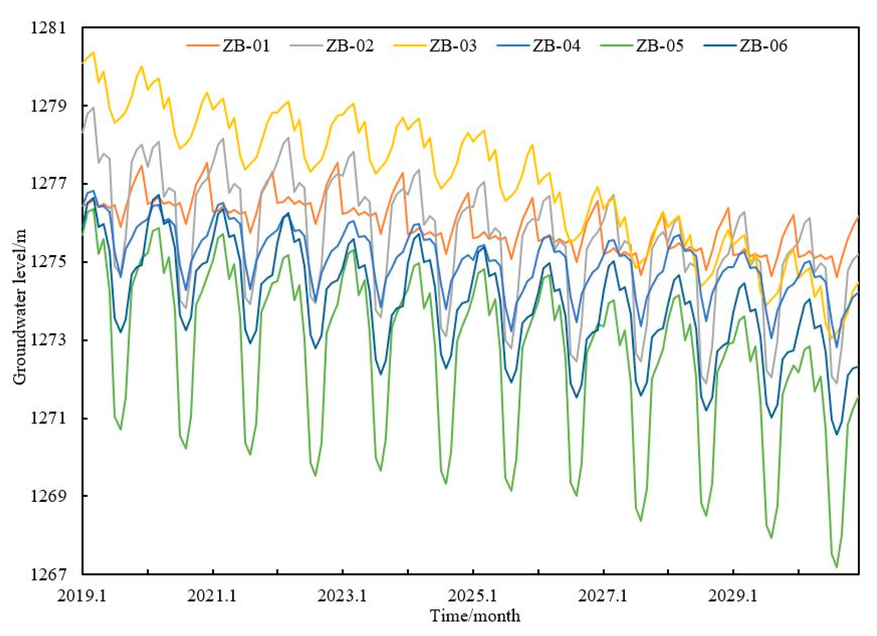
3.3. Groundwater Level Prediction under Different Mining Scenarios

The amount of groundwater exploitation should be optimized to ensure the sustainable utilization of groundwater in the study area [53]. The ABC-BP model was trained by continuously adjusting the input value of the exploitation amount and then to predict the groundwater levels of six monitoring wells under different mining scenarios. The prediction results of groundwater levels from 2019 to 2030 are summarized in Table 4 and Figure 10. Under the actual mining situation (40 million m3/year), groundwater level will be in the decline stage from 2019 to 2030, given the largest drop of 5.50 m. As the exploitation quantity was adjusted to 31 million m3/year, groundwater level only changed slightly and remained at a relatively stable value. Thereafter, groundwater level will enter the stable stage. As the exploitation quantity was adjusted to 22 million m3/year, groundwater level entered the recovery stage and gradually rose with a largest increase of 8.47 m and a rate of 0.71 m/a.
As evident in Figure 10, the variation trends of groundwater levels in the six monitoring wells are generally consistent under the same mining conditions. Groundwater level will gradually increase as exploitation quantity decreases. The groundwater system will gradually reach equilibrium as exploitation amount declines to 31 million m3/year, which is equal to the total recharge amount (Figure 10a). Therefore, an exploitation amount of 31 million m3/year is a reasonable value under the current conditions of the study area and can meet the requirements of the sustainable utilization of groundwater and the development of agriculture. Groundwater level will gradually rise as exploitation amount decreases to 22 million m3/year, and the damaged hydrological ecosystem will recover (Figure 10b). Nevertheless, an exploitation of 22 million m3/year will not guarantee the development of efficient local agriculture and economy. In conclusion, the most appropriate amount of groundwater exploitation for sustainable development in Yaoba Oasis is 31 million m3/year.
Feasible solutions such as strengthening the scientific management of water resources, implementing water-saving measures, improving the utilization rates of water resources, and adjusting crop planting structure, can effectively reduce the exploitation amount of groundwater. Subsequently, the results can change the status quo of mining. In future agricultural planning, the depressurization of groundwater exploitation is essential for balancing groundwater mining, replenishing groundwater resources, and achieving sustainable development for the agriculture, economy, and eco-environment of Yaoba Oasis.

4. Conclusions

An ABC-BP model with double hidden layers was proposed to simulate and predict the groundwater levels in Yaoba Oasis. The groundwater level data of six monitoring wells from January 2010 to December 2016 and January 2017 to December 2018 were used as training and test samples of the neural network, respectively. The data of the four major influencing factors, namely, recharge, exploitation, rainfall, and evaporation, obtained from January 2010 to December 2016, were used as input data. As constructed using a stepwise growing method and multi-trial algorithms, the topology structure of the ABC-BP model with double hidden layers was 4-7-3-1, which could overcome the over-fitting problem. The performance of the prediction model was determined by training and testing the ABC-BP and BP models on the sample data, respectively. The comparative analysis showed that the RE and MSE values in the optimal and worst training of the ABC-BP model were lower than the results in the optimal training of the BP model. In addition, the ABC-BP model obtained more consistent results and smaller MSE values after several training, compared with the BP model. Moreover, the ABC-BP model presented more accurate prediction results, the highest R2, and smaller MAE, REmax, and RMSE values than the PSO-BP, GA-BP, and BP models. In summary, the accuracy, convergence rate, and stabilization of the BP neural network with double hidden layers were considerably improved by the ABC algorithm by overcoming the low accuracy and slow convergence problems. Accordingly, the simulated values from January 2017 to December 2018 well fitted the measured values of the six monitoring wells during the training process of the proposed ABC-BP model.
The trained ABC-BP model with double hidden layers was applied to predict the groundwater levels in Yaoba Oasis from 2019 to 2030 under different mining scenarios. According to the prediction results, the groundwater levels will rise gradually as exploitation quantity decreases. Groundwater levels will enter the decline stage with a total decline range of 1.31 m to 5.50 m under the existing mining scenario (40 million m3/year), the stable stage with an exploitation amount of 31 million m3/year, and the recovery stage with an exploitation amount of 22 million m3/year. Therefore, the exploitation quantity of 31 million m3/year was found to be applicable for the sustainable development of groundwater resources in the study area.
The prediction of groundwater levels using the ABC-BP model in a typical oasis in the arid northwest region of China was realized in this study. The research results can guide the scientific utilization of groundwater and provide a novel approach for similar research in other arid oases with the same characteristics. Further investigation is suggested to forecast the daily groundwater level in the case of limited observed data, study the coupling between different influencing factors and groundwater level, and focus on the application of the ABC-BP model with different network structures in other hydrological fields.

Author Contributions

H.L. and Y.L. provided the original concept and methodology. C.Z. developed the program design and validation. M.Y. shared numerous comments to improve the quality of the study. S.L. gave valuable suggestions for the revision of this manuscript.

Funding

This research was supported by National Natural Science Foundation of China (Nos. 41630634 and 41877179) and the Fundamental Research Foundation of the Central Universities (No. 300102298706).

Acknowledgments

The authors are grateful to the local government and the hydrographic bureau in the Alax Left Banner of China for providing the monitoring data and for their helpful suggestions. The editor and reviewers are highly appreciated for providing positive and constructive comments and suggestions concerning this manuscript.

Conflicts of Interest

The authors declare no conflict of interest.

References

  1. Edmunds, W.M. Renewable and non-renewable groundwater in semi-arid and arid regions. Dev. Water Sci. 2003, 50, 265–280. [Google Scholar]
  2. Jiang, L.; Li, P.C.; Hu, A.Y.; Xu, Z.H. The groundwater chemical characteristics in the Yaoba oasis of Alxa area, Inner Mongolia. J. Arid Land Res. Environ. 2009, 23, 105–110. [Google Scholar]
  3. Chen, L.J.; Feng, Q. Geostatistical analysis of temporal and spatial variations in groundwater levels and quality in the Minqin oasis, Northwest China. Environ. Earth Sci. 2013, 70, 1367–1378. [Google Scholar] [CrossRef]
  4. Abliz, A.; Tiyip, T.; Ghulam, A.; Halik, Ü.; Ding, J.L.; Sawut, M.; Zhang, F.; Nurmemet, I.; Abliz, A. Effects of shallow groundwater table and salinity on soil salt dynamics in the Keriya oasis, northwestern China. Environ. Earth Sci. 2016, 75, 260. [Google Scholar] [CrossRef]
  5. Bao, C.; Fang, C.L. Water resources constraint force on urbanization in water deficient regions: A case study of the Hexi Corridor, arid area of NW China. Ecol. Econ. 2007, 62, 508–517. [Google Scholar] [CrossRef]
  6. Li, P.Y.; Qian, H.; Zhou, W.F. Finding harmony between the environment and humanity: An introduction to the thematic issue of the Silk Road. Environ. Earth Sci. 2017, 76, 105. [Google Scholar] [CrossRef]
  7. Shang, H.M.; Wang, W.K.; Dai, Z.X.; Duan, L.; Zhao, Y.Q.; Zhang, J. An ecology-oriented exploitation mode of groundwater resources in the northern Tianshan Mountains, China. J. Hydrol. 2016, 543, 386–394. [Google Scholar] [CrossRef]
  8. Chen, Y.N.; Li, W.H.; Xu, C.C.; Ye, Z.X.; Chen, Y.P. Desert riparian vegetation and groundwater in the lower reaches of the Tarim River basin. Environ. Earth Sci. 2014, 73, 547–558. [Google Scholar] [CrossRef]
  9. Alcalá, F.J.; Martínez-Valderrama, J.; Robles-Marín, P.; Guerrera, F.; Martín-Martín, M.; Raffaelli, G.; De León, J.T.; Asebriy, L. A hydrological-economic model for sustainable groundwater use in sparse-data drylands: Application to the amtoudi oasis in southern Morocco, northern Sahara. Sci. Total Environ. 2015, 537, 309–322. [Google Scholar] [CrossRef]
  10. Farnham, I.M.; Stetzenbach, K.J.; Singh, A.K.; Johannesson, K.H. Deciphering groundwater flow systems in oasis Valley, Nevada, using trace element chemistry, multivariate statistics, and geographical information system. Math. Geol. 2000, 32, 943–968. [Google Scholar] [CrossRef]
  11. Tweed, S.; Leblanc, M.; Cartwright, I.; Favreau, G.; Leduc, C. Arid zone groundwater recharge and salinisation processes; an example from the Lake Eyre Basin, Australia. J. Hydrol. 2011, 408, 257–275. [Google Scholar] [CrossRef]
  12. Chattopadhyay, S.; Bandyopadhyay, G. Artificial neural network with back propagation learning to predict mean monthly total ozone in Arosa, Switzerland. Int. J. Remote Sens. 2007, 28, 4471–4482. [Google Scholar] [CrossRef]
  13. Olawoyin, R. Application of back propagation artificial neural network prediction model for the PAH bioremediation of polluted soil. Chemosphere 2016, 161, 145–150. [Google Scholar] [CrossRef]
  14. Mandal, D.; Pal, S.K.; Saha, P. Modeling of electrical discharge machining process using back propagation neural network and multi-objective optimization using non-dominating sorting genetic algorithm-II. J. Mater. Process. Technol. 2007, 186, 154–162. [Google Scholar] [CrossRef]
  15. Kaveh, A.; Servati, H. Design of double layer grids using back propagation neural networks. Comput. Struct. 2001, 79, 1561–1568. [Google Scholar] [CrossRef]
  16. Neaupane, K.M.; Achet, S.H. Use of back propagation neural network for landslide monitoring: A case study in the higher Himalaya. Eng. Geol. 2004, 74, 213–226. [Google Scholar] [CrossRef]
  17. Métivier, M. Stock rate prediction using back propagation algorithm: Results with different number of hidden layers. J. Software Eng. 2007, 1, 13–21. [Google Scholar]
  18. Haviluddin, S.; Alfred, R. Daily network traffic prediction based on back propagation neural network. Aust. J. Basic and Appl. Sci. 2014, 8, 164–169. [Google Scholar]
  19. Akpinar, M.; Adak, M.F.; Yumusak, N. Forecasting natural gas consumption with hybrid neural networks-artificial bee colony. In Proceedings of the 2nd International Conference on Intelligent Energy and Power Systems (IEPS), Kyiv, Ukraine, 7–11 June 2016. [Google Scholar]
  20. Yu, F.; Xu, X.Z. A short-term load forecasting model of natural gas based on optimized genetic algorithm and improved BP neural network. Appl. Energy 2014, 134, 102–113. [Google Scholar] [CrossRef]
  21. Karaboga, D.; Basturk, B. A powerful and efficient algorithm for numerical function optimization: Artificial bee colony (ABC) algorithm. J. Glob. Optim. 2007, 39, 459–471. [Google Scholar] [CrossRef]
  22. Karaboga, D.; Basturk, B. On the performance of artificial bee colony (ABC) algorithm. Appl. Soft Comput. 2008, 8, 687–697. [Google Scholar] [CrossRef]
  23. Karaboga, D.; Akay, B. A survey: Algorithms simulating bee swarm intelligence. Artif. Intell. Rev. 2009, 31, 61–85. [Google Scholar]
  24. Su, C.H.; Xiang, N.; Chen, G.Y.; Wang, F. Water quality evaluation model based on artificial bee colony algorithm and BP neural network. Chin. J. Environ. Eng. 2012, 6, 699–704. [Google Scholar]
  25. Bullinaria, J.A.; Alyahya, K. Artificial bee colony training of neural networks: Comparison with back-propagation. Memetic Comp. 2014, 6, 171–182. [Google Scholar] [CrossRef]
  26. Irani, R.; Nasimi, R. Application of artificial bee colony-based neural network in bottom hole pressure prediction in underbalanced drilling. J. Pet. Sci. Eng. 2011, 78, 6–12. [Google Scholar] [CrossRef]
  27. Karaboga, D.; Akay, B. A comparative study of artificial bee colony algorithm. Appl. Math. Comput. 2009, 214, 108–132. [Google Scholar] [CrossRef]
  28. Garro, B.A.; Sossa, H.; Vazquez, R.A. Artificial neural network synthesis by means of artificial bee colony (ABC) algorithm. 2011 IEEE Congress of Evolutionary Computation (CEC) 2011, 30, 331–338. [Google Scholar]
  29. Nandy, S.; Sarkar, P.P.; Das, A. Training a feed-forward neural network with artificial bee colony based back propagation method. Int. J. Comput. Sci. Inf. Technol. 2012, 4, 652. [Google Scholar]
  30. Ozturk, C.; Karaboga, D. Hybrid artificial bee colony algorithm for neural network training. In Proceedings of the 2011 IEEE Congress of Evolutionary Computation (CEC), New Orleans, LA, USA, 5–8 June 2011; Volume 30, pp. 84–88. [Google Scholar]
  31. Qiu, H.X. The Salinization Mechanism of Groundwater and Simulation of Three-dimensional Water Quality, Inner Mongolia; Ocean University of Qingdao: Qingdao, China, 1997. [Google Scholar]
  32. Cui, G.Q.; Lu, Y.D.; Ce, Z.; Liu, Z.H.; Sai, J.M. Relationship between soil salinization and groundwater hydration in Yaoba Oasis, Northwest China. Water 2019, 11, 175. [Google Scholar] [CrossRef]
  33. Li, X.G.; Xia, W.; Lu, Y.D. Optimising the allocation of groundwater carrying capacity in a data-scarce region. Water SA 2010, 36, 451–460. [Google Scholar] [CrossRef]
  34. Zheng, C.; Lu, Y.D.; Guo, X.H.; Li, H.H.; Sai, J.M.; Liu, X.H. Application of HYDRUS-1D model for research on irrigation infiltration characteristics in arid oasis of northwest China. Environ. Earth Sci. 2017, 76, 785. [Google Scholar] [CrossRef]
  35. Li, Y.; Lu, Y.D.; Li, H.J.; Wang, J.K.; Jiang, L. Groundwater dynamic characteristics and the influence on vegetation variation in the yaoba oasis. Ground Water 2012, 4, 030. [Google Scholar]
  36. Ismailov, V.E. On the approximation by neural networks with bounded number of neurons in hidden layers. J. Math. Anal. Appl. 2014, 417, 963–969. [Google Scholar] [CrossRef]
  37. Yang, J.B.; Ni, F.S.; Wei, C.Y.; Zheng, Q.Y. Prediction of cutter-suction dredger production based on double hidden layer BP neural network. Comput. Digital Eng. 2016, 44, 1234–1237. [Google Scholar]
  38. Ding, H.; Dong, W.Y.; Wu, D.M. Water level prediction based on double hidden layer BP neural network based on LM algorithm. Stat. Decis. 2014, 15, 16–19. [Google Scholar]
  39. Xu, C.Y.; Xu, C.F. Optimization analysis of dynamic sample number and hidden layer node number based on BP neural network. In Proceedings of the Eighth International Conference on Bio-Inspired Computing: Theories and Applications (BIC-TA), HuangShan, China, 12–14 July 2013; Volume 212, pp. 687–695. [Google Scholar]
  40. Cui, D.W. Application of hidden multilayer BP neural network model in runoff prediction. J. China Hydrol. 2013, 33, 68–73. [Google Scholar]
  41. Sedki, A.; Ouazar, D.; El Mazoudi, E. Evolving neural network using real coded Genetic Algorithm for daily rainfall–runoff forecasting. Expert Syst. Appl. 2009, 36, 4523–4527. [Google Scholar] [CrossRef]
  42. Lu, Y.; Yang, J.; Wang, Q.; Huang, Z.J. The upper bound of the minimal number of hidden neurons for the parity problem in binary neural networks. Sci. China Inf. Sci. 2012, 55, 1579–1587. [Google Scholar] [CrossRef]
  43. Kacprzyk, J.; Pedrycz, W. Artificial neural network models. Springer Handbook of Computational Intelligence; Springer: Berlin, Germany, 2015; pp. 455–471. [Google Scholar]
  44. Seeley, T.D. The wisdom of the hive-The social physiology of honey bee colonies. Science 1996, 272, 907–908. [Google Scholar]
  45. Chen, S.Y.; Fang, G.H.; Huang, X.F.; Zhang, Y.H. Water quality prediction model of a water diversion project based on the improved Artificial bee colony–Backpropagation neural network. Water 2018, 10, 806. [Google Scholar] [CrossRef]
  46. Akay, B.; Karaboga, D. A modified artificial bee colony algorithm for real-parameter optimization. Inf. Sci. 2012, 192, 120–142. [Google Scholar] [CrossRef]
  47. Habbi, H.; Boudouaoui, Y.; Karaboga, D.; Ozturk, C. Self-generated fuzzy systems design using artificial bee colony optimization. Inf. Sci. 2015, 295, 145–159. [Google Scholar] [CrossRef]
  48. Pandey, A.; Srivastava, J.K.; Rajput, N.S.; Prasad, R. Crop parameter estimation of Lady finger by using different neural network training algorithms. Russ. Agric. Sci. 2010, 36, 71–77. [Google Scholar] [CrossRef]
  49. Saien, J.; Soleymani, A.R.; Bayat, H. Modeling fentonic advanced oxidation process decolorization of direct red 16 using artificial neural network technique. Desalin. Water Treat. 2012, 40, 174–182. [Google Scholar] [CrossRef]
  50. Taghavifar, H.; Mardani, A.; Mohebbi, A.; Taghavifar, H. Investigating the effect of combustion properties on the accumulated heat release of DI engines at rated EGR levels using the ANN approach. Fuel 2014, 137, 1–10. [Google Scholar] [CrossRef]
  51. Soleymani, A.R.; Saien, J.; Bayat, H. Artificial neural networks developed for prediction of dye decolorization efficiency with UV/K2S2O8 process. Chem. Eng. J. 2011, 170, 29–35. [Google Scholar] [CrossRef]
  52. Shah, H.; Tairan, N.; Garg, H.; Ghazali, R. A quick gbest guided Artificial bee colony algorithm for stock market prices prediction. Symmetry 2018, 10, 292. [Google Scholar] [CrossRef]
  53. Liu, J.Q.; Xie, X.M.; Ma, Z.Z.; Fang, G.H.; He, H.X.; Du, M.Y. A multiple-iterated dual control model for groundwater exploitation and water level based on the optimal allocation model of water resources. Water 2018, 10, 432. [Google Scholar] [CrossRef]
Figure 1. Map of Yaoba Oasis, Inner Mongolia Autonomous Region, China.
Water 11 00860 g001
Figure 2. Topology chart of the BP neural network with double hidden layers.
Water 11 00860 g002
Figure 3. Flowchart of the BP neural network based on the ABC algorithm. (modified from Su et al., 2012 [24]).
Water 11 00860 g003
Figure 4. Fitness of solutions in the ABC-BP model.
Water 11 00860 g004
Figure 5. Comparison curves of the absolute value of RE between the optimal and worst training of the ABC-BP and BP models.
Water 11 00860 g005
Figure 6. Variation curve of MSE in the optimal and worst training of the ABC-BP and BP models.
Water 11 00860 g006
Figure 7. Fitting curve of the measured and predicted values obtained using the ABC-BP, PSO-BP, GA-BP, and BP models.
Water 11 00860 g007
Figure 8. Fitting curve of the measured and predicted values of six monitoring wells obtained using the ABC-BP model.
Water 11 00860 g008aWater 11 00860 g008bWater 11 00860 g008c
Figure 9. Duration curves of groundwater levels in six monitoring wells from 2019 to 2030 under the existing mining scenario.
Water 11 00860 g009
Figure 10. Duration curves of the groundwater levels of six monitoring wells from 2019 to 2030 under different mining scenarios.
Water 11 00860 g010
Table 1. Error of network training with different numbers of nodes in the first and second hidden layers.
NeuronsErrorNeuronsErrorNeuronsErrorNeuronsErrorNeuronsErrorNeuronsErrorNeuronsError
3-30.864-30.765-30.576-30.347-30.018-30.139-30.22
3-40.834-40.715-40.416-40.277-40.038-40.199-40.26
3-50.764-50.655-50.386-50.237-50.068-50.249-50.30
3-60.704-60.635-60.236-60.127-60.148-60.299-60.38
3-70.654-70.485-70.206-70.077-70.198-70.349-70.47
3-80.574-80.455-80.166-80.047-80.258-80.429-80.53
3-90.524-90.325-90.136-90.027-90.298-90.469-90.56
Table 2. Comparison results of groundwater level prediction obtained using the ABC-BP, PSO-BP, GA-BP, and BP models.
Test SampleABC-BP ModelPSO-BP ModelGA-BP ModelBP Model
MonthMeasured Value
(m)
Predictive Value
(m)
Absolute ErrorPredictive Value
(m)
Absolute ErrorPredictive Value
(m)
Absolute ErrorPredictive Value
(m)
Absolute Error
2017/11280.241280.290.051280.430.191280.760.521279.55−0.69
2017/21280.491280.600.111280.950.461280.22−0.271280.830.34
2017/31280.551280.630.081280.710.161281.160.611281.651.10
2017/41279.911279.82−0.091279.54−0.371280.140.231279.02−0.89
2017/51280.021279.96−0.061280.560.541279.63−0.391280.210.19
2017/61279.251279.18−0.071279.420.171278.69−0.561280.110.86
2017/71278.611278.50−0.111278.20−0.411278.740.131279.270.66
2017/81279.031278.99−0.041278.82−0.211279.460.431279.260.23
2017/91279.141279.210.071279.320.181279.430.291278.72−0.42
2017/101279.591279.56−0.031279.34−0.251280.220.631279.46−0.13
2017/111280.061280.190.131279.74−0.321280.550.491280.640.58
2017/121280.271280.22−0.051280.550.281280.11−0.161280.380.11
2018/11279.641279.52−0.121279.950.311280.210.571279.980.34
2018/21279.811279.73−0.081280.280.471280.090.281279.66−0.15
2018/31279.921279.86−0.061280.050.131279.81−0.111280.290.37
2018/41279.161279.270.111279.250.091279.690.531279.600.44
2018/51279.441279.510.071278.93−0.511279.550.111279.21−0.23
2018/61278.481278.640.161278.740.261278.800.321277.57−0.91
2018/71278.121278.03−0.091278.470.351277.76−0.361278.650.53
2018/81278.261278.380.121278.15−0.111277.81−0.451278.510.25
2018/91278.421278.34−0.081278.720.301278.520.101279.030.61
2018/101278.791278.850.061278.64−0.151279.250.461278.48−0.31
2018/111279.311279.23−0.081279.550.241279.570.261279.570.26
2018/121279.561279.42−0.141279.990.431279.730.171279.990.43
Table 3. Comparison of four error representations of the ABC-BP, PSO-BP, GA-BP, and BP models.
Error RepresentationsName of Models
ABC-BPPSO-BPGA-BPBP
R20.9830.8640.8260.653
RMSE0.0920.3160.3900.533
MAE0.0860.2880.3520.460
REmax0.0130.0430.0490.086
Table 4. Analysis of variation for groundwater level from 2019 to 2030 different mining scenarios.
Monitoring WellLocationVariation Range of Groundwater Levels from 2019 to 2030 Under Different Mining Scenarios (m)
40 million m3/year31 million m3/year22 million m3/year
ZB-01North Central−1.310.136.73
ZB-02Central−2.810.017.24
ZB-03South Central−5.500.045.86
ZB-04West Central−1.790.078.47
ZB-05South−3.520.136.64
ZB-06South−2.610.226.11

